Toward Precision Black Hole Masses with ALMA:
NGC 1332 as a Case Study in Molecular Disk Dynamics

Abstract

We present first results from a program of Atacama Large Millimeter/submillimeter Array (ALMA) CO(2–1) observations of circumnuclear gas disks in early-type galaxies. The program was designed with the goal of detecting gas within the gravitational sphere of influence of the central black holes. In NGC 1332, the 0$\farcs$3-resolution ALMA data reveal CO emission from the highly inclined ($i\approx 83\arcdeg$) circumnuclear disk, spatially coincident with the dust disk seen in Hubble Space Telescope images. The disk exhibits a central upturn in maximum line-of-sight velocity reaching $\pm 500$ km s^-1 relative to the systemic velocity, consistent with the expected signature of rapid rotation around a supermassive black hole. Rotational broadening and beam smearing produce complex and asymmetric line profiles near the disk center. We constructed dynamical models for the rotating disk and fitted the modeled CO line profiles directly to the ALMA data cube. Degeneracy between rotation and turbulent velocity dispersion in the inner disk precludes the derivation of strong constraints on the black hole mass, but model fits allowing for a plausible range in the magnitude of the turbulent dispersion imply a central mass in the range $\sim(4-8)\times 10^{8}$ ${M}_{\odot}$. We argue that gas-kinematic observations resolving the black hole’s projected radius of influence along the disk’s minor axis will have the capability to yield black hole mass measurements that are largely insensitive to systematic uncertainties in turbulence or in the stellar mass profile. For highly inclined disks, this is a much more stringent requirement than the usual sphere-of-influence criterion.

1. Introduction

Direct measurement of the mass of a supermassive black hole (BH) in the center of a galaxy generally requires spatially resolved observations of tracer particles close enough to the BH that their orbits are dominated, or at least heavily influenced, by the gravitational potential of the BH. The “gold standards” of BH mass determinations are measurements for the Milky Way’s BH based on resolved stellar orbits (Ghez et al., 1998; Genzel et al., 2000; Ghez et al., 2008) and for the BH in NGC 4258 based on motions of H₂O megamasers resolved by very long-baseline interferometry (Miyoshi et al., 1995). There are two primary factors that make these the best measurements of BH masses. First, the observations are able to resolve kinematics at such small scales that the gravitational potential is overwhelmingly dominated by the BH itself. Second, the observations are able to measure the kinematics of individual test particles in orbit about the BH, rather than the combined and blended kinematics of a population of tracers having different orbital trajectories.

Aside from the special cases of the Milky Way, NGC 4258, and a small number of other megamaser disk galaxies (e.g. Kuo et al., 2011), most of the $\sim 100$ dynamical detections of BHs come from observations and modeling of spatially resolved stellar or gas kinematics, mostly from the Hubble Space Telescope (HST) or large ground-based telescopes equipped with adaptive optics; for a review of methods and results see Kormendy & Ho (2013). Due to the limitations of angular resolution, these observations do not isolate individual test particles; rather, they rely on the combined line-of sight kinematics of stars in the galaxy’s bulge, or of gas clouds in a rotating disk, in both cases modified by the blurring effect of the instrumental point-spread function. The stellar-dynamical method is most widely applicable, in that stars are always present as dynamical tracers in galaxy nuclei, but the construction of orbit-based dynamical models is a formidable challenge. Models have recently evolved toward greater complexity due to a growing recognition that the derived BH masses can be sensitive to the treatment of the dark matter halo (Gebhardt & Thomas, 2009), triaxial structure (van den Bosch & de Zeeuw, 2010), and stellar mass-to-light ratio gradients in the host galaxy (McConnell et al., 2013).

Measurements of BH mass from ionized gas kinematics are conceptually and technically simpler since the method relies on modeling circular rotation of a thin disk rather than modeling the full stellar orbital structure of an entire galaxy, and early measurements done with HST spectroscopy demonstrated the potential of this technique (Harms et al., 1994; Ferrarese et al., 1996). In contrast to stellar dynamics, the dynamics of a thin circular disk at small radii are relatively insensitive to the galaxy’s dark matter halo or to stellar mass-to-light gradients. However, ionized gas-dynamical measurements suffer from a separate and significant set of systematic uncertainties. Ionized gas disks often have a substantial turbulent velocity dispersion ($\sigma_{\mathrm{turb}}$), sometimes up to hundreds of km s^-1 (van der Marel & van den Bosch, 1998; Barth et al., 2001b; Verdoes Kleijn et al., 2006; Walsh et al., 2010), which must be accounted for in modeling the disk dynamics. In some cases, the dynamical effect of this turbulence can affect the estimated BH mass at the factor of $\sim 2$ level compared with masses inferred from thin disk modeling if turbulent pressure support is neglected. Incorporating turbulent pressure support has been done using approximations based on point-particle dynamics, either by applying the formalism of asymmetric drift (Barth et al., 2001b) or by applying the Jeans equation to model a kinematically hot, vertically extended rotating disk (Neumayer et al., 2007). These methods are not intrinsically well-suited to gas-dynamical systems, but more rigorous approaches are still lacking.

Another source of systematic uncertainty is the extended mass distribution of stars: when the BH’s gravitational radius of influence ($r_{\mathrm{g}}$; the radius within which $M_{\mathrm{BH}}>0.5M_{\mathrm{total}}$) is not highly resolved, errors in determination of the stellar mass profile can strongly impact the accuracy of $M_{\mathrm{BH}}$ measurements. In many gas-dynamical measurements done with HST, $r_{\mathrm{g}}$ has been just marginally resolved, and only in the very best cases such as M87 (Macchetto et al., 1997; Walsh et al., 2013) is $r_{\mathrm{g}}$ so highly resolved that the BH dominates the mass profile at the smallest observed scales. This problem is exacerbated by the very optically thick dust present in most gas-dynamical targets, which impedes the measurement of the intrinsic stellar luminosity profile. Despite much early enthusiasm and a large number of HST orbits invested in the method, ionized gas dynamics has not produced a very large number of robust BH masses, in part due to the fact that many galaxies targeted for HST observations did not exhibit clean rotational kinematics in the circumnuclear gas (Ho et al., 2002; Hughes et al., 2003; Noel-Storr et al., 2007; Walsh et al., 2008).

In some galaxies, near-infrared ro-vibrational H₂ emission lines from circumnuclear disks of warm molecular gas can be detected. With adaptive optics, it is possible to map the kinematics of H₂ disks at high resolution and constrain BH masses (e.g., Neumayer et al., 2007; Hicks & Malkan, 2008; Scharwächter et al., 2013; den Brok et al., 2015). However, the warm molecular gas in active galactic nuclei often appears to be somewhat kinematically disturbed or irregular, even when the gas is in overall rotation about the BH (Mazzalay et al., 2014), and it has not generally been possible to derive highly precise constraints on BH masses using it as a tracer.

Cold molecular gas has the potential to emerge as an important new dynamical tracer for BH mass measurement, enabled largely by the recent construction of the Atacama Large Millimeter/submillimeter Array (ALMA). The basic principles of BH mass measurement via molecular gas dynamics are essentially identical to those used for ionized gas-dynamical measurements, but cold molecular gas offers several key advantages in terms of the physical structure of circumnuclear disks and the practical aspects of carrying out a dynamical measurement. Similar to ionized gas disks, the dynamics of rotating molecular disks close to and within $r_{\mathrm{g}}$ are essentially unaffected by the host galaxy’s large-scale dark matter halo or possible triaxial structure, thus avoiding two of the most significant uncertainties associated with stellar-dynamical BH detection in early-type galaxies (ETGs). Crucially, cold molecular gas tends to have a smaller turbulent velocity dispersion than the ionized gas in the same galaxy, making it a better tracer of the circular velocity (Young et al., 2008; Davis et al., 2013a) and more amenable to accurate dynamical modeling.

About 10% of ETGs contain well-defined, regular, flat, and round circumnuclear dust disks that can be seen easily in HST images (e.g., van Dokkum & Franx, 1995; Tran et al., 2001; Laine et al., 2003; Lauer et al., 2005). In cases where these disks have associated ionized components, they have been targets for gas-dynamical BH mass measurements with HST, but some dust disks have very weak or undetectable optical line emission. The optical morphology can provide a clear indication of dense gas in rotation about the galaxy center, and such disks are potentially the best and most promising targets for measurement of BH masses with ALMA. Pre-ALMA CO observations of molecular gas disks in ETGs illustrated that well-defined, round dust disks are generally associated with regular, circular rotation in the molecular gas, although interferometric observations were not generally able to probe angular scales as small as $r_{\mathrm{g}}$ in nearby galaxies (e.g., Okuda et al., 2005; Young et al., 2008; Alatalo et al., 2013). The first proof of concept for BH mass measurement via CO kinematics was presented by Davis et al. (2013b), who used the Combined Array for Research in Millimeter-wave Astronomy (CARMA) to observe NGC 4526 at 0$\farcs$25 resolution, just sufficient to resolve $r_{\mathrm{g}}$. ALMA now offers the possibility of routinely carrying out molecular-line observations that resolve $r_{\mathrm{g}}$, opening up a major new avenue for determination of BH masses in galaxy nuclei.

While it has long been anticipated that ALMA will enable BH mass measurements based on spatially resolved molecular-line kinematics (e.g., Maiolino, 2008), it is not yet clear how widely applicable this new method will prove to be. The potential of the method depends crucially on the ability to identify targets having cleanly rotating gas within $r_{\mathrm{g}}$, with a high enough surface brightness for molecular line emission on these scales to be detected and mapped in reasonable exposure times. In ALMA Cycle 2, we began a program of observations of ETGs in order to pursue the goal of obtaining BH mass measurements. The first stage of this program involves observations of the CO(2–1) line at $\sim 0\farcs 3$ resolution to search for evidence of rapid rotation within the BH sphere of influence. Targets were selected based on the presence of well-defined, round circumnuclear dust disks as seen in HST images. For galaxies showing regularly rotating disks with high-velocity CO emission from within $r_{\mathrm{g}}$, deeper and higher-resolution observations can then be proposed in order to obtain highly precise measurements of $M_{\mathrm{BH}}$.

A total of seven ETGs were observed in our Cycle 2 programs, and observations for the full sample will be presented in a forthcoming paper. Here, we present the first results from this project, an examination of the circumnuclear disk kinematics in NGC 1332. NGC 1332 is an S0 or E galaxy with a bulge stellar velocity dispersion of 328 km s^-1 (for a detailed description of its morphology and classification see Kormendy & Ho, 2013). It contains a highly inclined and opaque circumnuclear dust disk that is visible in HST images. The BH mass in NGC 1332 has previously been measured using two different techniques. Rusli et al. (2011) found $M_{\mathrm{BH}}=(1.45\pm 0.20)\times 10^{9}$ ${M}_{\odot}$ (at 68% confidence) from stellar-dynamical modeling of VLT adaptive-optics data. Humphrey et al. (2009) modeled the hydrostatic equilibrium of the X-ray emitting gas in NGC 1332 using data from the Chandra X-ray Observatory and derived a smaller central mass of $M_{\mathrm{BH}}=0.52_{-0.28}^{+0.41}\times 10^{9}$ ${M}_{\odot}$ (at 90% confidence). The discrepancy between these two measurements provides additional motivation to attempt to measure $M_{\mathrm{BH}}$ via molecular gas dynamics. While the nearly edge-on disk inclination makes NGC 1332 a challenging target for gas-dynamical studies, it is a rare example of a galaxy that can serve as a test case for comparison of three independent methods to measure its BH mass, making it a compelling target for ALMA observations. Following the detection of CO emission from within $r_{\mathrm{g}}$ in these Cycle 2 data, higher-resolution (0$\farcs$04) observations of NGC 1332 have been approved for ALMA’s Cycle 3. This paper provides an initial look at the circumnuclear disk kinematics in this galaxy at the 0$\farcs$3 resolution of the Cycle 2 data. This resolution is sufficient to resolve the BH’s radius of influence if $M_{\mathrm{BH}}>8\times 10^{8}$ ${M}_{\odot}$.

The recession velocity of NGC 1332 as measured from optical data is $1550\pm 29$ km s^-1 (da Costa et al., 1991). We adopt a distance of 22.3 Mpc for consistency with Rusli et al. (2011), while Humphrey et al. (2009) used a slightly smaller distance of 21.3 Mpc.

2. Observations

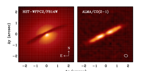
Figure 1.— Left: HST WFPC2 F814W ($I$-band) image of the NGC 1332 nucleus and dust disk, displayed with logarithmic stretch. Right: ALMA CO(2-1) image, summed over all frequency channels of the data cube and displayed with linear stretch. The ellipse at lower right illustrates the FWHM size of the ALMA synthesized beam.

As part of Program 2013.1.0229.S, ALMA observed NGC 1332 on 2014 September 1 in a frequency band centered on the redshifted ¹²CO(2-1) 230.538 GHz line at $\nu_{\mathrm{obs}}=229.37$ GHz (in ALMA Band 6). The minimum and maximum baselines of the array were 33.7 m and 1.1 km, respectively, and the on-source integration time was 22.7 min. Observations were processed using version 4.2.2, r30721 of the Common Astronomy Software Application (CASA; McMullin et al., 2007) package and version 31266 of the standard ALMA pipeline. This produced a data cube spanning a field of view of 21″$\times$21″ with 0.07″ spatial pixels (corresponding to 7.6 pc pixel^-1), and a separate continuum image having the same pixel scale. Use of Briggs weighting with robustness parameter 0.5 yields a synthesized beam with major and minor axis FWHM sizes of $0\farcs 319$ and $0\farcs 233$ and major axis position angle 78$\fdg$4, giving a geometric mean resolution of 0$\farcs$27 corresponding to 29.2 pc in NGC 1332. The data cube contains 60 frequency channels with spacing 15.4 MHz, or velocity spacing 20.1 km s^-1 relative to the frequency of the CO(2–1) line at the NGC 1332 systemic velocity. The RMS noise level as measured in line-free regions of the data cube is 0.4 mJy beam^-1 per channel. The overall flux scale for the data was set by an observation of the quasar J0334$-$4008, for which we adopt a 10% uncertainty (see, e.g., the Appendix of ALMA Partnership et al., 2015) in the pipeline-reported value of 0.76 Jy at 234.2 GHz.

Line emission is visible in 52 channels in the data cube, spanning a full velocity width of 1040 km s^-1. Figure 1 shows the ALMA CO image of NGC 1332, summed over all frequency channels of the data cube. CO emission originates from a region corresponding closely to the optically thick dust disk with 2$\farcs$2 angular radius, as seen in an archival HST WFPC2 F814W ($I$-band) image. There is no significant CO emission detected above the level of the background noise at any location outside the circumnuclear disk. The disk’s CO surface brightness distribution exhibits a dip within the innermost $r\lesssim 0\farcs 2$, but even in this region CO emission is clearly detected. The continuum image reveals a marginally resolved source at the disk center with flux density $8.75\pm 0.04$ mJy; we assume an additional 10% uncertainty in this value based on the uncertainty in the overall flux calibration.

3. CO emission properties and disk kinematics

Figure 2 illustrates the integrated CO emission profile over this region, which exhibits a symmetric double-horned shape with peaks separated by 840 km s^-1. To examine the spatially resolved kinematics, we fit the line profile at each spatial pixel using a sixth-order Gauss-Hermite function (van der Marel, 1994). The S/N was sufficient to obtain successful fits at each pixel over an elliptical region having major and minor axis lengths of 4$\farcs$3 and 0$\farcs$7. Outside this region, the CO flux drops rapidly to below the level of the noise.

Figure 2.— CO(2–1) line profile integrated over an elliptical region having major and minor axis lengths of $4\farcs 3$ and $0\farcs 7$. The error bar at lower left shows the background noise level summed in quadrature over this integration region.

Figure 3 shows the spatially resolved kinematic moment maps for the line-of-sight velocity centroid ($v_{\mathrm{LOS}}$, measured relative to the systemic velocity), the dispersion $\sigma_{\mathrm{LOS}}$, and the higher-order Gauss-Hermite moments $h_{3}$ through $h_{6}$. The odd-numbered moments $h_{3}$ and $h_{5}$ describe asymmetric departures from a Gaussian profile, while the even-numbered moments $h_{4}$ and $h_{6}$ quantify symmetric deviations from a Gaussian shape. The $v_{\mathrm{LOS}}$ map illustrates the fact that the NGC 1332 disk is in orderly rotation overall. Beam smearing of the disk’s velocity field is particularly severe given the disk’s nearly edge-on inclination. At 0$\farcs$3 resolution, the disk’s projected semi-minor axis is essentially unresolved, and low-velocity emission “piles up” into the line profiles along the disk major axis. Consequently, high-velocity emission from gas in rotation near the disk center is spatially blended with a substantial amount of low-velocity emission from foreground and background regions along the disk surface.

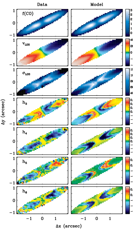
Figure 3.— Maps of CO intensity, $v_{\mathrm{LOS}}$, $\sigma_{\mathrm{LOS}}$, $h_{3}$, $h_{4}$, $h_{5}$, and $h_{6}$ measured from Gauss-Hermite fits to the data and model cubes. The left panels show kinematic moment maps of the ALMA data, and the right panels show the best-fitting model for the flat $\sigma_{\mathrm{turb}}$ profile having $M_{\mathrm{BH}}=6.0\times 10^{8}$ ${M}_{\odot}$, as described in §5.2. The model CO intensity map gives the integral of the CO line profile at each spatial pixel in the modeled data cube. Units for the CO surface brightness map are Jy beam^-1 km s^-1, and units for the $v_{\mathrm{LOS}}$ and $\sigma_{\mathrm{LOS}}$ maps are km s^-1. In this and subsequent figures, line-of-sight velocities are shown relative to the systemic velocity 1559 km s^-1 determined from the best-fitting model. The higher-order moment coefficients $h_{3}$ through $h_{6}$ are dimensionless.

The $v_{\mathrm{LOS}}$ map for NGC 1332 shows a relatively steep velocity gradient across the nucleus from the southeastern (redshifted) to northwestern (blueshifted) side of the disk, but without central high-velocity emission. High-velocity emission is present near the disk center, but as a sub-dominant contribution to the line profiles. The primary signature of the disk’s central rise in rotation speed is in the $h_{3}$ map, which shows very strong blueward and redward asymmetries on opposite sides of the disk center. The $\sigma_{\mathrm{LOS}}$ map has an “X” shape typical of inclined rotating disks, with peak line-of-sight velocity dispersion $\sim 120$ km s^-1. This “X” shape comes from rotational broadening and beam smearing in regions of the disk exhibiting a steep gradient in line-of-sight velocity. It is also possible that a portion of the spatial variation in observed line width could be due to a radial gradient in the disk’s intrinsic turbulent velocity dispersion, but dynamical modeling is required to distinguish the separate contributions of beam smearing and turbulent velocity gradients. The $h_{5}$ and $h_{6}$ maps are noisy but still contain coherent structure tracing the same features as $h_{3}$ and $h_{4}$.

To examine the kinematic position angle (PA) as a function of radius in the disk, we used the kinemetry method of Krajnović et al. (2006), applying kinemetry to the measured $v_{\mathrm{LOS}}$ map. The kinemetry routine fits a harmonic expansion to $v_{\mathrm{LOS}}$ along elliptical annuli. Its output includes, at each semi-major axis distance $R$, the kinematic position angle $\Gamma$, the axis ratio $q$ of the kinematic ellipse, the first harmonic coefficient $k_{1}$ (equivalent to the major axis line-of-sight velocity amplitude), and the ratio $k_{5}/k_{1}$. The $k_{5}$ coefficient quantifies deviations from pure rotation, and the presence of strong features in the $k_{5}/k_{1}$ map can indicate the existence of multiple kinematic components. The kinematic PA $\Gamma$ refers to the kinematic major axis and is defined here such that PA=0° would correspond to a north-south orientation for the disk major axis with the northern side of the disk redshifted. We use the term kinematic major axis to refer to the locus of points of maximum line-of-sight velocity amplitude on each elliptical annulus, which is equivalent to the line of nodes for an inclined, flat circular disk seen in projection. The kinematic minor axis refers to the locus of points at which $v_{\mathrm{LOS}}$ is equal to the systemic velocity $v_{\mathrm{sys}}$. In a flat circular disk, the kinematic major and minor axes will be seen as orthogonal straight lines on the sky, but in the presence of warping, radial flows, or elliptical orbits, this is in general no longer the case. (See Wong, Blitz, & Bosma 2004 for a detailed discussion of the observable signatures of noncircular or warped kinematics in gaseous disks.)

As described by Krajnović et al. (2008), galaxies having multiple kinematic components are typically characterized by either abrupt changes in $q$ or $\Gamma$ (with $\Delta q>0.1$ or $\Delta\Gamma>10\arcdeg$), or a double-peaked $k_{1}$ profile, or the presence of a distinct peak in the $k_{5}$ profile at which $k_{5}/k_{1}$ ¿ 0.02. A kinematic twist is identified if $\Gamma$ varies smoothly with radius with a rotation of $>10\arcdeg$.

The kinemetry results are shown in Figure 4. The kinematic PA $\Gamma$ ranges from 128° at $r=0\farcs 22$ (within one resolution element of the galaxy nucleus) to 117° at the outer edge of the disk, which can be characterized as a mild kinematic twist. The $k_{5}/k_{1}$ ratio is below 0.02 at all radii and does not contain any strong features. Overall, the modest radial variation in $\Gamma$ and $q$, and the flat $k_{5}/k_{1}$ profile with magnitude of $\sim 1\%$, indicate that the NGC 1332 disk kinematics are consistent with coherent disk rotation as the dominant kinematic structure. If $r_{\mathrm{g}}$ were well resolved, $k_{1}$ would exhibit a central quasi-Keplerian ($v\sim r^{-0.5}$) decline with increasing distance from the nucleus, but instead we see a smooth monotonic rise in $k_{1}$ as a function of $R$. This is an indication that $v_{\mathrm{LOS}}$ does not in itself provide direct evidence for a compact central mass; beam smearing hides the central high-velocity emission in the higher-order velocity moment maps.

Figure 4.— Kinemetry for the NGC 1332 line-of-sight velocity ($v_{\mathrm{LOS}}$) map. From top to bottom, the panels illustrate the kinematic PA $\Gamma$, the flattening $q$, the $k_{1}$ coefficient (equivalent to the amplitude of $v_{\mathrm{LOS}}$ along the disk major axis), and the ratio $k_{5}/k_{1}$.

We also extract a position-velocity diagram (PVD) as another method to visualize the kinematics. We constructed the PVD by rotating each frequency slice of the data cube clockwise by 27° so that the kinematic PA at the largest measured radius was oriented horizontally, and then extracting a four-pixel wide swath through the data cube (corresponding to one resolution element) along the disk major axis. Figure 5 shows the PVD, which illustrates a smooth and continuous distribution of emission across the full range of velocities present in the disk. The central high-velocity emission is clearly seen in the form of a slight upturn in the locus of maximum line-of-sight speed on either side of the nucleus. This central velocity upturn is relatively faint and only seen within $\pm 0\farcs 8$ of the nucleus, it only spans 3–4 velocity channels above the level of the flat outer envelope in rotation velocity, and it is spatially blended with a much larger amount of emission spanning the entire velocity range present in the disk. This PVD structure may be contrasted with the case of an observation in which $r_{\mathrm{g}}$ is well resolved: in that situation, the central velocity upturn would be seen as a narrow locus of emission, rather than as the outer envelope of a broad distribution of velocities extending down to zero. Nevertheless, the velocity rise seen within the innermost $\sim 0\farcs 5$ is the expected signature of a compact central massive object that dominates the gravitational potential at small radii. Although the CO surface brightness map shows a central dip in brightness within the innermost $r<0\farcs 2$, the observed velocity structure provides evidence that the intrinsic CO-emitting region extends to scales within the black hole’s sphere of influence.

From the PVD, we can extract an estimate of the enclosed gravitating mass within one resolution element of the galaxy nucleus. At a distance of four pixels (0$\farcs$28) from the galaxy center, corresponding to $r=30$ pc, the maximum velocity seen in the PVD is $\approx 480$ km s^-1. If this maximum velocity is equated with the circular speed at $r=30$ pc, the implied enclosed mass is $M(r)\approx 1.6\times 10^{9}$ ${M}_{\odot}$, which can then be taken as an upper limit to $M_{\mathrm{BH}}$ since it includes both the BH and the stellar mass enclosed within this radius. A caveat to this simple estimate is that the CO line profiles may be broadened by turbulence in the molecular gas disk, in which case the outermost velocity envelope seen in the PVD would give an upper limit to the line-of-sight circular velocity.

The PVD structure also helps to clarify why the integrated CO line profile in Figure 2 is so strongly double peaked. The flat outer velocity envelope to the PVD at $r\sim 0\farcs 8-2\farcs 2$ indicates that the galaxy’s rotation curve is fairly flat over this range of radii. As a result, there is a large amount of CO emission at line-of-sight velocities in a narrow range around $\pm 400$ km s^-1 from gas along the disk’s major axis.

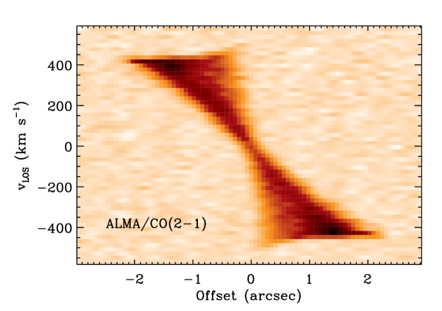
Figure 5.— Position-velocity diagram along the disk major axis, from a four-pixel extraction width. Data are displayed with a linear stretch.

The total CO(2-1) flux of the disk is $37.7\pm 0.3$ Jy km s^-1, with an additional 10% uncertainty in the flux scale. We can use this flux value to obtain an estimate of the total molecular gas mass of the disk by applying a CO-to-H₂ conversion factor $\alpha_{\mathrm{CO}}$ (e.g., Bolatto et al., 2013). Following Carilli & Walter (2013), we convert from observed flux to luminosity to obtain $L^{\prime}_{\mathrm{CO(2-1)}}=(1.14\pm 0.11)\times 10^{7}$ K km s^-1 pc². The CO-to-H₂ conversion is most reliably calibrated in terms of the luminosity of the CO(1–0) emission line, which we do not have for NGC 1332. Following Sandstrom et al. (2013), we assume an intensity ratio $R_{21}\equiv L^{\prime}_{\mathrm{CO(2-1)}}/L^{\prime}_{\mathrm{CO(1-0)}}=0.7$. For the sample of 18 ETGs studied by Crocker et al. (2012), the median CO intensity ratio is $R_{21}=0.76$ with standard deviation of 0.23, consistent with our adopted value of 0.7. Then, a standard value of $\alpha_{\mathrm{CO}}=3.1$ ${M}_{\odot}$ pc^-2 (K km s^-1)^-1 derived for nearby galaxies and including a factor of 1.36 correction for helium (Sandstrom et al., 2013) leads to an estimated molecular gas mass of $M_{\mathrm{gas}}=\alpha_{\mathrm{CO}}L^{\prime}_{\mathrm{CO(1-0)}}=(5.0\pm 0.5)\times 10^{7}$ ${M}_{\odot}$. Sandstrom et al. (2013) find that within the central kpc of galaxies, $\alpha_{\mathrm{CO}}$ is typically a factor of $\sim 2$ below this adopted standard value, however, and in some cases the value of $\alpha_{\mathrm{CO}}$ in galaxy centers is an order of magnitude lower than the average. If this trend applies to ETGs as well, then the actual gas mass in the disk could be several times lower than this simple estimate. The circumnuclear disk of NGC 1332 may have physical conditions very different from the environments in which $\alpha_{\mathrm{CO}}$ has been calibrated, and in regions of high density and high optical depth the standard assumptions of the CO-to-H₂ conversion method may be invalid (Bolatto et al., 2013). We therefore consider the gas mass derived above as merely a rough estimate.

4. Dynamical Modeling

4.1. Method

We modeled the kinematics of a flat circular disk following the same approach used for ionized gas disks observed with HST (Macchetto et al., 1997; Barth et al., 2001b; Walsh et al., 2010). The calculation begins with a mass model consisting of the central point mass $M_{\mathrm{BH}}$ and the extended mass profile of stars in the host galaxy $M_{\star}(r)$, representing the mass enclosed within radius $r$. The mass profile $M_{\star}(r)$ is determined from an empirically measured and deprojected luminosity profile, with the stellar mass-to-light ratio $\Upsilon$ as a free parameter.

We neglect the possible contribution of dark matter, which is expected to be extremely small relative to stellar mass on scales comparable to the circumnuclear disk radius. The mass model of NGC 1332 from Humphrey et al. (2009) indicates a total enclosed dark matter mass of $\approx 10^{8}$ ${M}_{\odot}$ within $r<250$ pc, two orders of magnitude lower than the stellar mass enclosed at this scale. Our model does not include the mass of the gas disk itself, since our estimate of the total molecular gas mass is $\sim 5\times 10^{7}$ ${M}_{\odot}$ within $r<250$ pc.

A circular, flat disk in rotation about the galaxy center has rotation speed given by $v_{\mathrm{rot}}(r)=[GM(r)/r]^{1/2}$ where $M(r)=M_{\mathrm{BH}}+M_{\star}(r)$. The line-of-sight velocity at each point in the model disk is then determined for a given inclination angle $i$ and a major axis orientation angle $\Gamma$ (for details see Macchetto et al., 1997; Barth et al., 2001b). The model is constructed on a spatial grid that is highly oversampled relative to the ALMA spatial pixel size, because a given pixel near the disk center can contain gas spanning a substantial velocity range. In the models, each ALMA pixel is subdivided into an $s\times s$ grid of sub-pixel elements. At each sub-pixel element in the grid, we model the emergent line profile as a Gaussian, with central velocity given by the projected rotation velocity at that point, and with some turbulent linewidth $\sigma_{\mathrm{turb}}$. We discuss the possible radial variation of $\sigma_{\mathrm{turb}}$ in §4.3.

The line profiles at each location must be weighted by the CO surface brightness at the corresponding point in the disk. The available information on the CO surface brightness distribution of the disk is simply the velocity-integrated CO image as shown in Figure 1. However, this is an image of the disk modified by beam smearing, and the model requires an image of the intrinsic surface brightness distribution. Ideally one would want a CO surface brightness map at the same resolution as the $s\times s$ sub-pixel sampling of the model grid, but such information is not available. Lacking knowledge of the CO surface brightness distribution on subpixel scales, the line profiles at each sub-pixel grid point contributing to a given ALMA spatial pixel were normalized to have equal fluxes. Then, the subsampled data cube was rebinned to the spatial pixel scale of the ALMA data by averaging each $s\times s$ set of sub-pixel line profiles to form a single profile. The line profiles are calculated on a grid of 20.1 km s^-1 pixel^-1, corresponding to the velocity sampling of the ALMA data cube.

In order to scale the line profile of each spatial pixel to its appropriate flux level, we used a deconvolved CO surface brightness map. We deconvolved the CO image shown in Figure 1 using five iterations of the Richardson-Lucy algorithm (Richardson, 1972; Lucy, 1974) implemented in IRAF, where the deconvolution was carried out with an elliptical Gaussian point-spread function (PSF) matching the specifications of the ALMA synthesized beam. The choice of five iterations of the deconvolution algorithm is somewhat arbitrary: this produced an adequately sharpened image, and larger numbers of iterations began to produce noticeable artifacts by amplifying background noise. In the model calculation, the line profile at each pixel was then normalized to match the flux at the corresponding pixel in the deconvolved flux map. To allow for any possible mismatch in flux normalization between the deconvolved flux map and the original ALMA data cube, we multiply the flux map by a scaling factor $f_{0}$ that is a free parameter in the model fits. In practice, the best-fitting value of $f_{0}$ is very close to unity.

Each frequency slice of the modeled cube is then convolved with the ALMA synthesized beam, modeled as an elliptical Gaussian, producing a simulated data cube analogous to the ALMA data. Since we rebin the high-resolution model cube to the ALMA pixel resolution prior to carrying out the PSF convolution, there is little time penalty for carrying out the initial computation of line profiles on an oversampled pixel grid with $s$ as high as 10, and it is feasible to carry out model optimizations with the line profiles computed at much finer spatial sampling ($s=50$ for example). PSF convolution is often the most time-consuming step of gas-dynamical model calculations, particularly if the convolution is carried out on an oversampled pixel grid.

Free parameters in the model include $M_{\mathrm{BH}}$ and $\Upsilon$, the $x$ and $y$ centroid positions of the BH, the systemic velocity $v_{\mathrm{sys}}$, the inclination and orientation angles of the disk $i$ and $\Gamma$, the flux-normalization factor $f_{0}$ applied to the CO flux map, and the parameters describing the run of $\sigma_{\mathrm{turb}}$ as a function of radius in the disk (see §4.3; this requires up to three parameters depending on the choice of $\sigma_{\mathrm{turb}}$ model).

4.2. Stellar Mass Profile

The stellar mass profile $M_{\star}(r)$ is an essential ingredient in the dynamical modeling, and is determined by measuring and deprojecting the galaxy’s surface brightness profile. Ideally, this should be measured from imaging data having angular resolution at least as high as the spectroscopic data. Near-infrared observations are strongly preferred, especially for galaxies having dusty nuclei. The only available HST image of NGC 1332 is the WFPC2 F814W image shown in Figure 1, and the dust disk is extremely optically thick in the $I$ band.

Rusli et al. (2011) used a combination of seeing-limited $R$-band data on large scales, and $K$-band AO data on small scales ($<4\farcs 5$), to measure the stellar luminosity profile of NGC 1332; they masked out the central dust disk in extracting the galaxy’s light profile. Their model was then deprojected under the assumption of axisymmetric structure and an inclination of 90°. We used this same mass profile (kindly provided by J. Thomas) in order to carry out a direct comparison between our gas-dynamical modeling and the stellar-dynamical results of Rusli et al. (2011). The version of the mass profile provided (which we denote $M_{R\star}$) was the average of the best-fitting stellar-dynamical models over the four quadrants of the VLT integral-field kinematic data, and corresponds to a stellar mass-to-light ratio in the $R$ band of $\Upsilon_{R}=7.35$. In our models, we incorporated this mass profile directly, multiplied by a mass-to-light scaling factor $\gamma$ (a free parameter in the model fits), such that $M_{\star}(r)=\gamma M_{R\star}(r)$ and the resulting mass-to-light ratio is $\Upsilon_{R}=7.35\gamma$. As described below, our best fits converged on values of $\gamma$ very close to unity, indicating that our gas-dynamical model fitting finds close agreement with the stellar mass distribution measured by Rusli et al. (2011).

As a consistency check, we also measured a stellar luminosity profile from the archival HST data. The HST observation was taken as two individual 320 s exposures with the galaxy nucleus on the PC chip of the WFPC2 camera (0$\farcs$0456 arcsec pixel^-1), and we combined the two exposures using the IRAF/STSDAS task crrej. We measured the galaxy’s surface brightness profile from the PC image, first masking point sources, globular clusters, and the dust disk. The disk was masked over the radial range 0$\farcs$1–2$\farcs$3. The central four pixels, where dust extinction appears less severe, were retained in order to anchor the radial profile measurement at the galaxy’s nucleus, but the measurement then gives a lower limit to the central surface brightness due to dust extinction along the nuclear line of sight.

The surface brightness profile was fit using a 2D multi-Gaussian expansion (MGE) using the MGE_FIT_SECTORS package (Cappellari, 2002), using eight Gaussian components. The MGE expansion requires a PSF model, and we modeled the PC F814W PSF using an MGE fit to a synthetic PSF generated using Tiny Tim (Krist et al., 2011). Deprojection of the MGE model was done assuming that the galaxy bulge is an oblate spheroid with inclination 83° (based on fits to the ALMA kinematics described below). CCD counts were converted to $I$-band solar units accounting for a Galactic foreground extinction of $A_{I}=0.049$ mag (Schlafly & Finkbeiner, 2011) to give the $I$-band luminosity profile $L_{I}(r)$. The mass profile is then given by $M_{\star}(r)=\Upsilon_{I}L_{I}(r)$, where $\Upsilon_{I}$ is the $I$-band mass-to-light ratio.

Figure 6 shows the enclosed stellar mass profile $M_{\star}(r)$ from Rusli et al. (2011) and the profile measured from the HST F814W image. In both cases, the mass-to-light ratio normalization is based on the best-fitting result for models assuming a spatially uniform value of $\sigma_{\mathrm{turb}}$, as described in §4.3. The $I$-band stellar mass profile implies a lower stellar mass than the $R$+$K$ band profile from Rusli et al. (2011). The most plausible explanation is that this mass deficit is the result of dust absorption by the circumnuclear disk in the $I$-band HST image, which could not be entirely masked out. We therefore choose to use the Rusli et al. (2011) profile for our final model fits. At the outer edge of the disk at $r=240$ pc, the enclosed stellar mass reaches $10^{10}$ ${M}_{\odot}$, so the BH is expected to make a small contribution to the total enclosed mass at this scale.

Figure 6.— Enclosed stellar mass profiles $M_{\star}(r)$ as measured by Rusli et al. (2011) (solid curve) and as measured from the HST WFPC2 F814W image (dashed curve). The mass-to-light ratio in each case is based on the best-fitting dynamical model with a spatially uniform value of the turbulent velocity dispersion $\sigma_{\mathrm{turb}}$. The vertical dotted line corresponds to the 0$\farcs$27 resolution of the ALMA data.

4.3. Turbulent Velocity Dispersion Profile

To model the CO line profiles, some assumption must be made regarding the intrinsic velocity dispersion of the gas. The thermal contribution to the linewidth for cold molecular gas will be extremely small: Bayet et al. (2013) find kinetic temperatures of typically $\sim 10-20$ K for molecular gas in ETG disks. Ideally, with angular resolution high enough to resolve individual giant molecular clouds (GMCs) within the disk, the turbulent velocity dispersion of individual GMCs can be measured. In a range of environments, the highest linewidths observed in individual GMCs correspond to $\sigma_{\mathrm{turb}}\approx 30-40$ km s^-1 (Leroy et al., 2015). The closest analog to NGC 1332 having observations of high enough resolution to isolate individual GMCs is NGC 4526, where CO(2–1) observations from CARMA were able to resolve 103 individual GMCs (Utomo et al., 2015). In NGC 4526, most of the individual GMCs were found to have $\sigma_{\mathrm{turb}}\approx 5-10$ km s^-1, and the highest-dispersion clouds have $\sigma_{\mathrm{turb}}\approx 25$ km s^-1. For NGC 1332, the 0$\farcs$3 resolution of our ALMA data shows a very smooth distribution of CO emission across the disk surface, and much higher angular resolution would be required in order to identify individual clouds within the disk or measure their velocity dispersions directly.

In the outer regions of the NGC 1332 disk, the CO emission profiles are very narrow. At the largest radii along the disk major axis, the lines are unresolved as observed in the 20 km s^-1 velocity channels, with measured linewidths of $\sigma\approx 10-20$ km s^-1 from the Gauss-Hermite fits. Toward the inner regions of the disk, the linewidths rise to a maximum of $\sigma=120$ km s^-1, with the largest widths observed at locations about 0$\farcs$3–0$\farcs$4 on either side of the nucleus along the disk major axis. In this central region, the line profiles are extremely asymmetric with broad, extended wings. As will be shown below, most or all of this rise in observed linewidth can be explained by beam smearing of unresolved rotation. There remains the possibility, however, of a genuine increase in the gas turbulent velocity dispersion toward the disk center. One issue in the model construction is that if the pixel oversampling factor $s$ is too low, the models can have a tendency to require a spuriously high value of $\sigma_{\mathrm{turb}}$ to compensate for inadequate spatial sampling of rotational velocity gradients. It is crucial, therefore, to ensure that the models are computed on a grid with sufficient spatial sampling that $\sigma_{\mathrm{turb}}$ is not biased toward higher values than actually occur in the disk.

If the molecular gas in the NGC 1332 disk is arranged in unresolved discrete clouds then the CO line width from an individual cloud is the result of the internal turbulent velocity dispersion within the cloud, rotation of the cloud as a whole, and shear due to galactic differential rotation. Additionally, random motions of clouds (either in-plane or vertical) will contribute to the observed line widths. Since our observations do not resolve individual clouds, our data cannot distinguish among these contributions, and we use the term “turbulence” to refer to the combination of all processes responsible for the emergent line width from a given location at the disk surface. In their study of the NGC 4526 GMC population, Utomo et al. (2015) found that the energy in turbulent motion dominated over internal rotational energy for nearly all of the resolved clouds.

To explore how the model fits depend on the assumed turbulent velocity dispersion profile and allow for possible radial gradients in turbulence, we ran models using the following prescriptions for $\sigma_{\mathrm{turb}}(r)$.

Flat: The simplest parameterization is $\sigma_{\mathrm{turb}}$ = constant, allowing $\sigma_{\mathrm{turb}}$ to be a free parameter in the model fits.

Exponential: Following a typical prescription used in ionized gas dynamics, we used a model of the form $\sigma_{\mathrm{turb}}=\sigma_{0}\exp(-r/r_{0})+\sigma_{1}$, where $\sigma_{0}$, $\sigma_{1}$, and $r_{0}$ are free parameters. Model fits consistently drove the value of $\sigma_{1}$ to zero, so this parameter was discarded from final fits. To prevent the line profile widths from becoming arbitrarily narrow, we enforced a minimum value of $\sigma_{\mathrm{turb}}=1$ km s^-1.

Gaussian: The largest observed linewidths are seen at locations slightly offset from the disk center, suggesting that a $\sigma_{\mathrm{turb}}$ model with a central depression could provide a better fit to the data. As a simple model allowing for a central plateau or dip in $\sigma_{\mathrm{turb}}$, we used a Gaussian profile: $\sigma_{\mathrm{turb}}=\sigma_{0}\exp[-(r-r_{0})^{2}/(2\mu^{2})]+\sigma_{1}$, where $\sigma_{0}$, $\sigma_{1}$, $r_{0}$, and $\mu$ are free parameters. Again, we found that model fits drove $\sigma_{1}$ to zero and we removed this parameter from the final model runs, and enforced a minimum value of $\sigma_{\mathrm{turb}}=1$ km s^-1. The parameter $r_{0}$ was allowed to vary over positive and negative values for maximum freedom in fitting the data. Positive values were preferred by the fits, producing a central dip in the turbulent velocity dispersion.

In §5, we present a comparison of model fitting results using each of these parameterizations for $\sigma_{\mathrm{turb}}$. We emphasize that none of these prescriptions for $\sigma_{\mathrm{turb}}$ represents a physically motivated model. The disk’s actual $\sigma_{\mathrm{turb}}$ profile could be considerably different from any of these prescriptions (and might not be axisymmetric), but the data do not provide sufficient information to justify modeling $\sigma_{\mathrm{turb}}$ with anything much more complex than these simple parameterizations.

4.4. Model Optimization

The output of each model computation for a given parameter set is a simulated data cube having the same spatial and velocity sampling as the ALMA data. Thus, the models can be fitted directly to the ALMA data cube to optimize the fit by $\chi^{2}$ minimization. We fit models using the amoeba downhill simplex method implemented in IDL.

For model fits to the observed data cube, we fit models only to the spatial pixels within the elliptical region illustrated in Figure 3, using 52 frequency channels at each spatial pixel spanning the full width of the CO emission line. To determine $\chi^{2}$ by direct comparison of the modeled cube with the data, an estimate is required for the flux uncertainty at each pixel in the data. The simplest way to estimate the noise level would be to determine the standard deviation of pixel values in emission-free regions of the data cube. However, the background noise in the data exhibits strong correlations among neighboring pixels, on angular scales similar to the synthesized beam size. A proper calculation of $\chi^{2}$ in the presence of strongly correlated errors requires the computation and inversion of the covariance matrix of the data uncertainties (e.g., Gould, 2003). We attempted to construct a covariance matrix by using “blank”, emission-free regions of the data cube to determine the pixel-to-pixel correlations in the background noise. Within the elliptical fitting region, there are 523 individual spatial pixels. We found that numerical errors in constructing and inverting the covariance matrix rendered the $\chi^{2}$ calculation highly unstable.

We then opted for a simplified approach to computing $\chi^{2}$. The background noise correlations are strong on scales comparable to the synthesized beam, of size $\sim 0\farcs 3$, while the pixel size is 0$\farcs$07. We rebinned the data by spatially averaging the flux over $4\times 4$ pixel blocks within each frequency channel, yielding approximately one rebinned pixel per synthesized beam. This process averages over the mottled pattern in the background noise seen at the original pixel resolution, producing a data cube in which the background noise is nearly uncorrelated among neighboring pixels. In this block-averaged data cube, we measured the standard deviation of pixel values in blank regions to determine the noise level for use in measuring $\chi^{2}$. The RMS noise level in the $4\times 4$ block-averaged data is 0.3 mJy beam^-1 (compared with 0.4 mJy beam^-1 in the original data). The fact that the noise in the block-averaged data is nearly as large as in the full-resolution data (rather than scaling as $1/\sqrt{n}$ where $n$ is the number of binned pixels) reflects the strong local correlations in the pixel values of the full-resolution data. Then, for each model iteration, the calculated model at the original ALMA pixel scale was similarly block-averaged over $4\times 4$ pixel regions to compare with the block-averaged data. In the rebinned data, we calculate $\chi^{2}$ over 49 block-averaged spatial pixels and 52 frequency channels at each pixel, for a total of 2548 data points.

5. Modeling Results

5.1. Initial tests

As an initial test to examine the impact of different values of the oversampling factor $s$, we ran fits with models having a flat turbulent velocity dispersion and oversampling factors of $s=1$, 2, 3, 4, 5, 10, 20, and 50. All model parameters were free in these initial fits. Figure 7 illustrates the results of varying $s$. An oversampling factor of $s=2$ was the bare minimum required in order to obtain modeled P–V diagrams having smooth structure similar to the observed PVD. The models converged on consistent results for $\chi^{2}$ and for the free parameters when the oversampling factor was greater than $s=4$. We choose $s=10$ for our final model fits since there appears to be no discernible benefit to using higher values of $s$, while using $s>10$ significantly increases the time for model computation. For $s=10$, the fits converged on $M_{\mathrm{BH}}=6.0\times 10^{8}$ ${M}_{\odot}$, with $\sigma_{\mathrm{turb}}=24.7$ km s^-1 and $\Upsilon_{R}=7.25$.

Figure 7.— Best-fitting values of $M_{\mathrm{BH}}$ and $\sigma_{\mathrm{turb}}$, and the corresponding $\chi^{2}$ values, for models with flat $\sigma_{\mathrm{turb}}$ and oversampling factor $s$ ranging from 1 to 50. The number of degrees of freedom in the fit is 2540.

We also ran a model fit in which $\chi^{2}$ was computed using the full-resolution ALMA data cube and model, rather than the $4\times 4$ pixel block-averaged version. With $s=10$, the results for the best-fitting parameters were virtually identical to the block-averaged fits: we found best-fit values of $M_{\mathrm{BH}}=6.0\times 10^{8}$ ${M}_{\odot}$, $\sigma_{\mathrm{turb}}=24.3$ km s^-1, and $\Upsilon_{R}=7.26$. In all subsequent models fitted to the data cube, we apply the $4\times 4$ block averaging to the data and models when calculating $\chi^{2}$ in order to alleviate any possible issues related to correlated errors in the background noise, but the block averaging does not appear to have an appreciable impact on the best-fitting parameter values.

5.2. Model fits with flat $\sigma_{\mathrm{turb}}$

With oversampling fixed to $s=10$, we ran initial model optimizations for a two-dimensional grid over a range of fixed values of $M_{\mathrm{BH}}$ (from 0 to $2\times 10^{9}$ ${M}_{\odot}$ in increments of $10^{8}$ ${M}_{\odot}$) and $\sigma_{\mathrm{turb}}$ (from 5 to 50 km s^-1 in increments of 5 km s^-1). All other parameters were allowed to vary freely. Figure 8 shows contours of constant $\Delta\chi^{2}$ relative to the best-fitting model at $M_{\mathrm{BH}}=6.0\times 10^{8}$ ${M}_{\odot}$ and $\sigma_{\mathrm{turb}}=25$ km s^-1, where the minimum $\chi^{2}$ was 11173.4. The value of $\chi^{2}$ climbs very steeply as the parameters depart from these best-fitting values.

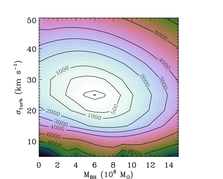
Figure 8.— Contours of constant $\Delta\chi^{2}$ as a function of $M_{\mathrm{BH}}$ and $\sigma_{\mathrm{turb}}$, for the flat $\sigma_{\mathrm{turb}}$ profile. The minimum $\chi^{2}$ value of 11173.4 (for 2540 degrees of freedom) is obtained at $M_{\mathrm{BH}}=6\times 10^{8}$ ${M}_{\odot}$ and $\sigma_{\mathrm{turb}}=25$ km s^-1. The two innermost contours correspond to $\Delta\chi^{2}=10$ and 100. Models were calculated over a grid with increments of $10^{8}$ ${M}_{\odot}$ and 5 km s^-1.

For a closer examination of the parameter space around the best fit, we then ran a grid of models with finer sampling in $M_{\mathrm{BH}}$ ranging from 0 to $2\times 10^{9}$ ${M}_{\odot}$ in which $\sigma_{\mathrm{turb}}$ and other parameters were left free. We found that the disk orientation parameters $i$ and $\Gamma$ converged to very narrow ranges that were insensitive to the fixed $M_{\mathrm{BH}}$ values in these fits, with inclination $i=83\arcdeg-84\arcdeg$, and kinematic PA $\Gamma=117\fdg 44-117\fdg 67$, consistent with the kinematic PA determined by kinemetry for the outer disk. The disk’s centroid velocity and position parameters also converged tightly, with $v_{\mathrm{sys}}=1559\pm 1$ km s^-1, and the best-fitting $x$ and $y$ positions for the disk’s dynamical center remaining constant to within $\pm 0.1$ ALMA pixels over the range of $M_{\mathrm{BH}}$ values tested.

Figure 9.— Curves of $\chi^{2}$ as a function of $M_{\mathrm{BH}}$ for models calculated with the flat, exponential, and Gaussian $\sigma_{\mathrm{turb}}$ profiles.

For these model fits, the best-fitting value for $\sigma_{\mathrm{turb}}$ ranged from 23 to 27 km s^-1, slightly larger than one velocity channel in the ALMA data cube. The $R$-band mass-to-light ratio is anticorrelated with $M_{\mathrm{BH}}$, and for $M_{\mathrm{BH}}$ ranging from 0 to $2\times 10^{9}$ ${M}_{\odot}$, $\Upsilon_{R}$ ranged from 8.10 to 5.31.

The best-fitting model with flat $\sigma_{\mathrm{turb}}$ is found at $M_{\mathrm{BH}}=6.02\times 10^{8}$ ${M}_{\odot}$. In this model fit, $\Upsilon_{R}=7.25$ and $\sigma_{\mathrm{turb}}=24.7$ km s^-1. With 2540 degrees of freedom, the model has $\chi^{2}=11171.8$ and $\chi^{2}_{\nu}=4.40$, indicating a poor fit to the data overall. Figure 9 shows $\chi^{2}$ as a function of $M_{\mathrm{BH}}$ for these model fits. If we were to adopt the usual criterion of $\Delta\chi^{2}=6.63$ corresponding to a 99% confidence range, we would obtain an extremely narrow range of $(5.66-6.34)\times 10^{8}$ corresponding to an uncertainty of $\pm 6\%$ about the best-fitting value of $M_{\mathrm{BH}}$. However, since $\chi^{2}_{\nu}$ is much greater than unity for the best fit, standard $\Delta\chi^{2}$ intervals are not directly applicable and we do not consider these confidence intervals to be meaningful. If we were to inflate the noise uncertainties by a factor of 2 in order to achieve $\chi^{2}_{\nu}\approx 1$ for the best fit, the $\Delta\chi^{2}=6.63$ interval would correspond to a slightly broader mass range of $(5.3-6.7)\times 10^{8}$ ${M}_{\odot}$.

Figure 3 illustrates the kinematic moment maps for this model fit, which reproduce the overall features of the observed moment maps reasonably well although there are clearly systematic differences in detail. The model $h_{3}$ map approximately matches the sign reversal in $h_{3}$ seen on either side of the nucleus: the line profiles at small radii have very extended high-velocity tails, while at large radii along the disk major axis the line profiles have extended low-velocity tails. Since the modeled line profiles are assumed to be intrinsically Gaussian at each location in the disk before beam smearing, the departures from Gaussian profiles in the modeled data cube can only result from blending of line profiles originating from different locations in the disk. The close match between the observed and modeled moment maps confirms that the complex line profile shapes in the data are predominantly the result of rotational broadening and beam smearing.

Figure 10 shows the best-fitting model PVDs for models calculated with $M_{\mathrm{BH}}$ fixed to 0, $6.0\times 10^{8}$, and $1.45\times 10^{9}$ ${M}_{\odot}$; the last value is equal to the best-fitting mass from Rusli et al. (2011). The model with $M_{\mathrm{BH}}=0$ clearly fails in that it does not have a central upturn in maximum rotation velocity. At $M_{\mathrm{BH}}=6\times 10^{8}$ ${M}_{\odot}$, the model has a central velocity upturn similar to that seen in the data, and at $M_{\mathrm{BH}}=1.45\times 10^{9}$ ${M}_{\odot}$ the central upturn is too prominent to match the data.

One noticeable aspect of these model PVDs is that the CO linewidths in the outer disk are broader than in the data. This can also be seen in Figure 11, which illustrates line profiles extracted from the PVD at eight spatial locations. The models follow the overall shapes of the observed line profiles fairly well, even near the disk center at $\pm 0\farcs 21$ (or $\pm 3$ pixels) where the profiles are extremely broad and asymmetric. In the outermost slices through the PVD, the modeled CO profiles are clearly broader than the observed profiles.

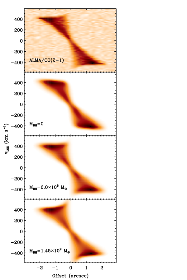
Figure 10.— PVDs for models with flat $\sigma_{\mathrm{turb}}$ profiles compared with the ALMA data. The three models displayed are the best-fitting models with flat $\sigma_{\mathrm{turb}}$ for $M_{\mathrm{BH}}$ fixed to 0, $6.0\times 10^{8}$, and $1.45\times 10^{9}$ ${M}_{\odot}$. The best-fitting $\sigma_{\mathrm{turb}}$ values are 27.7, 24.7, and 24.0 km s^-1, respectively.

To examine the possibility that the model optimization is somehow biased towards high values of $\sigma_{\mathrm{turb}}$, we created a PVD for the best-fitting model having $\sigma_{\mathrm{turb}}=10$ km s^-1; at this value, the intrinsic CO linewidths would be unresolved by the ALMA data. For $\sigma_{\mathrm{turb}}=10$ km s^-1, the best-fitting BH mass is $8.0\times 10^{8}$ ${M}_{\odot}$. The value of $\chi^{2}$ for this model is 16063.5, dramatically worse than the best-fitting model at $M_{\mathrm{BH}}=6.0\times 10^{8}$ ${M}_{\odot}$ (as can be seen in Figure 8). Figure 12 compares the PVD of this model with the model having $M_{\mathrm{BH}}=6.0\times 10^{8}$ ${M}_{\odot}$ and $\sigma_{\mathrm{turb}}=24.7$ km s^-1. It is somewhat striking that the $\sigma_{\mathrm{turb}}=10$ km s^-1 model appears to match some aspects of the observed PVD distinctly better than does the best-fitting model. In particular, the $\sigma_{\mathrm{turb}}=10$ km s^-1 model appears to more closely match the observed narrow linewidths in the outer disk, and the shape of the inner velocity upturn at small radii. The model is, however, a much worse match to the observed PVD overall, as clearly indicated by its much larger $\chi^{2}$ value. The line-profile cuts through the modeled PVD, shown in Figure 11, help to clarify how this model fails to match the data. At positions of $\pm 0\farcs 7$ from the disk center, there is a “pile-up” of emission at $v_{\mathrm{LOS}}=\pm 420$ km s^-1 causing a spike in emission that is not present in the data at these locations. Larger values of $\sigma_{\mathrm{turb}}$ in the inner regions of the disk tend to reduce the amplitude of this emission peak, matching the data more closely.

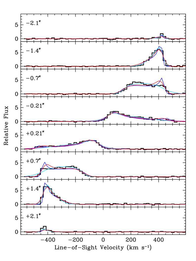
Figure 11.— Line profiles measured by extracting single-column cuts through the PVD at eight spatial locations. The PVD is based on a four pixel wide extraction along the disk major axis. The observed PVD is shown in black. Modeled profiles are as follows. Red: The best-fitting model with flat $\sigma_{\mathrm{turb}}$. Blue: Model with flat $\sigma_{\mathrm{turb}}=10$ km s^-1. Magenta: Best-fitting model with exponential $\sigma_{\mathrm{turb}}$. Cyan: Best-fitting model with Gaussian $\sigma_{\mathrm{turb}}$. The models with exponential and Gaussian $\sigma_{\mathrm{turb}}$ profiles are closely overlapping at most locations. Numerical labels in each panel show the offset in arcseconds from the galaxy nucleus along the major axis.

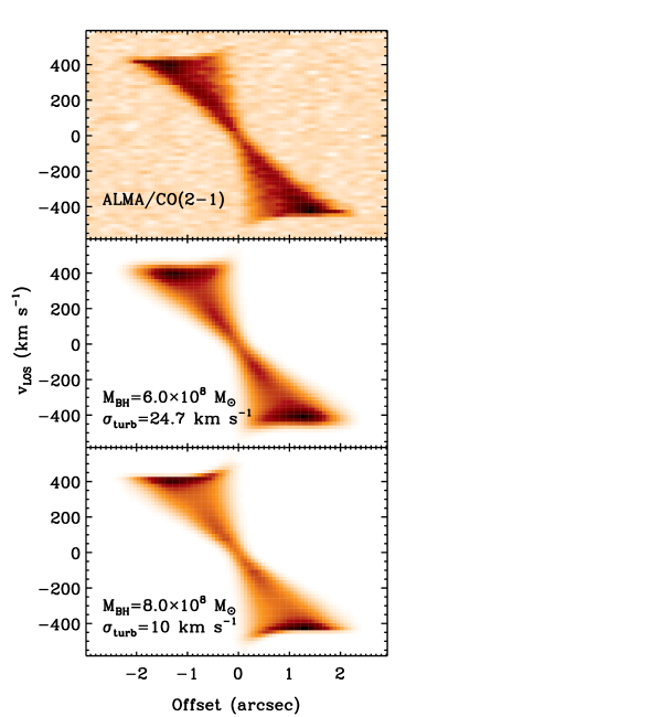
Figure 12.— PVDs for models with flat $\sigma_{\mathrm{turb}}$ profiles. The middle panel shows the overall best-fitting model with flat $\sigma_{\mathrm{turb}}$, having $M_{\mathrm{BH}}=6.0\times 10^{8}$ ${M}_{\odot}$ and $\sigma_{\mathrm{turb}}=24.7$ km s^-1. The lower panel shows the best fitting model having a fixed $\sigma_{\mathrm{turb}}=10$ km s^-1. For this model, $M_{\mathrm{BH}}=8.0\times 10^{8}$ ${M}_{\odot}$.

5.3. Model fits with other $\sigma_{\mathrm{turb}}$ profiles

Since the best-fitting model with $\sigma_{\mathrm{turb}}=24.7$ km s^-1 clearly overpredicts the CO linewidths in the outer disk, while models with smaller values of $\sigma_{\mathrm{turb}}$ lead to dramatically poorer fits to the data overall, we conclude that the flat $\sigma_{\mathrm{turb}}$ profile is not a sufficient description of the disk’s turbulent velocity dispersion profile. To allow for radial gradients in $\sigma_{\mathrm{turb}}$ and attempt to achieve more satisfactory fits with lower $\chi^{2}$, we ran grids of models using the exponential and Gaussian $\sigma_{\mathrm{turb}}$ profiles. As before, models were run over a set of fixed values of $M_{\mathrm{BH}}$, with all other parameters allowed to vary freely.

Figure 9 shows $\chi^{2}$ as a function of $M_{\mathrm{BH}}$ for both the exponential and Gaussian $\sigma_{\mathrm{turb}}$ profiles. The most basic result is that the more complex $\sigma_{\mathrm{turb}}$ profiles lead to better fits overall with significantly lower $\chi^{2}$, but taken at face value they imply a BH mass much lower than the value derived from the flat $\sigma_{\mathrm{turb}}$ fits.

For the exponential $\sigma_{\mathrm{turb}}$ profile, when all parameters were allowed to vary freely, the model fits converged on a best-fitting BH mass of zero (Figure 9, middle panel), with $\Upsilon_{R}=7.94$. For this best-fitting model ($\chi^{2}=7790.8$ for 2539 degrees of freedom) the central value of $\sigma_{\mathrm{turb}}$ becomes quite high, with $\sigma_{0}=268$ km s^-1 and $r_{0}=60.7$ pc. The PVD for this model, shown in Figure 14, helps to illustrate why this model produces a much lower $\chi^{2}$ than models with flat $\sigma_{\mathrm{turb}}$. At radii between 1″ and 2″, the PVD of the exponential $\sigma_{\mathrm{turb}}$ model is a much better match to the observed PVD structure than any of the flat $\sigma_{\mathrm{turb}}$ models. At the same time, the fit with $M_{\mathrm{BH}}=0$ does not have a central velocity upturn. Instead, the smallest radii in the PVD are characterized by an increase in linewidth due to the high central $\sigma_{\mathrm{turb}}$ value. In effect, the model fit is unable to distinguish between rotation and dispersion in the inner disk, while in the outer disk the fits clearly prefer having a gradient in $\sigma_{\mathrm{turb}}$ allowed by the exponential model, as opposed to the flat $\sigma_{\mathrm{turb}}$ models. Qualitatively, the structure of the PVD is a very poor match to the central velocity upturn of the data, but the $\chi^{2}$ minimization result is dominated by structure at larger radii in the PVD.

While a central turbulent velocity dispersion of 268 km s^-1 is probably unphysically high for molecular gas, it is not clear whether any specific prior constraint on $\sigma_{0}$ would be justifiable. To examine the interplay between $M_{\mathrm{BH}}$ and constraints imposed on the central value of $\sigma_{\mathrm{turb}}$, we ran a grid of models over a range of fixed values of $M_{\mathrm{BH}}$ and of the central turbulent velocity dispersion $\sigma_{0}$. The results are shown in Figure 13. We find that when $\sigma_{0}$ is restricted to low values in the range $\sim 10-30$ km s^-1, similar to the range of turbulent velocity dispersions seen in resolved GMCs in nearby galaxies, the model fits converge on $M_{\mathrm{BH}}$ in the range $\sim(6-8)\times 10^{8}$ ${M}_{\odot}$. However, higher fixed values of $\sigma_{0}$ produce fits with significantly lower BH masses. Additionally, restricting $\sigma_{0}$ to low values produces much worse fits overall in comparison with the free $\sigma_{0}$ fits: for example, when $\sigma_{0}$ is fixed to 25 km s^-1, the best fit is found for $M_{\mathrm{BH}}=6.0\times 10^{8}$, with $\chi^{2}=11083.0$.

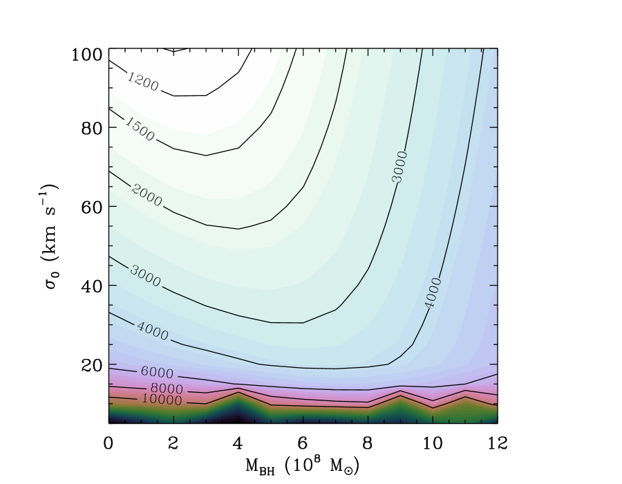
Figure 13.— Contours of constant $\Delta\chi^{2}$ for models with the exponential $\sigma_{\mathrm{turb}}$ profile, as a function of $M_{\mathrm{BH}}$ and the central turbulent velocity dispersion $\sigma_{0}$. For $\sigma_{0}\leq 50$ km s^-1, the best-fitting BH mass is $\sim(4-8)\times 10^{8}$ ${M}_{\odot}$, but higher fixed values of $\sigma_{0}$ result in model fits with lower $M_{\mathrm{BH}}$. If $\sigma_{0}$ is left as a free parameter, the best-fitting model has $\sigma_{0}=268$ km s^-1, and $\chi^{2}=7790.8$ for 2539 degrees of freedom; the $\Delta\chi^{2}$ values plotted in this figure are relative to that best-fitting value.

This illustrates the most severe problem in fitting models to the NGC 1332 data: once we allow for the possibility of a radial gradient in $\sigma_{\mathrm{turb}}$, the inferred value of $M_{\mathrm{BH}}$ is directly dependent upon the assumed upper limit to $\sigma_{\mathrm{turb}}$ in the central region of the disk. There does not appear to be any clear way to circumvent this problem, since the line profiles are so strongly affected by rotational broadening that $\sigma_{\mathrm{turb}}$ cannot be directly measured or constrained independently of a dynamical model for the disk rotation. Larger values of $\sigma_{\mathrm{turb}}$ directly lead to significantly lower $\chi^{2}$ for the overall model fit, and by the $\chi^{2}$ criterion the model fits strongly prefer a model with no BH but with a central $\sigma_{\mathrm{turb}}$ that is probably unphysically large. It is also important to note that for the highest values of $\sigma_{\mathrm{turb}}$ reached in these models, the thin disk assumption would break down, invalidating the basic premises of our dynamical modeling. If the disk were actually highly turbulent in its central regions, the turbulent pressure support would have to be accounted for in determining $M_{\mathrm{BH}}$. This would raise $M_{\mathrm{BH}}$ to a non-zero value.

We also ran a separate grid of models with the exponential $\sigma_{\mathrm{turb}}$ profile and $s=25$, to test whether the high central $\sigma_{\mathrm{turb}}$ values might be the result of insufficient model resolution of the disk’s central kinematics at $s=10$. The model fitting results were essentially identical to the $s=10$ case.

As an attempt to examine a model in which $\sigma_{\mathrm{turb}}$ possesses a radial gradient without a central peak, we ran model fits using the Gaussian $\sigma_{\mathrm{turb}}$ profile. Since the Gaussian centroid can be radially offset from the disk center, this model allows for a central depression in $\sigma_{\mathrm{turb}}$. For a grid of model fits over fixed values of $M_{\mathrm{BH}}$, Figure 9 (right panel) shows the best-fitting $\chi^{2}$ as a function of $M_{\mathrm{BH}}$. Similar to the exponential profile models, we find that the best fit with the Gaussian $\sigma_{\mathrm{turb}}$ profile is obtained for $M_{\mathrm{BH}}=0$ and $\Upsilon_{R}=7.96$, and the best-fitting $\chi^{2}$ value in this case is 7499.7 for 2538 degrees of freedom. In this model, the Gaussian $\sigma_{\mathrm{turb}}$ parameters are $\sigma_{0}=100.3$ km s^-1, $\mu=78.9$ pc, and $r_{0}=14.5$ pc. This small value of $r_{0}$ indicates that the Gaussian peak is very close to the disk center, and the central dip in $\sigma_{\mathrm{turb}}$ is essentially unresolved. Trial fits demonstrated that if $\sigma_{0}$ is restricted to values well below 100 km s^-1, the inferred $M_{\mathrm{BH}}$ value from $\chi^{2}$ minimization is directly determined by the constraint imposed on $\sigma_{0}$, similar to the situation for the exponential $\sigma_{\mathrm{turb}}$ profile. The PVD for this model is displayed in Figure 14, and Figure 11 shows the CO line profiles at several locations along the disk major axis for the best-fitting exponential and Gaussian $\sigma_{\mathrm{turb}}$ models.

The best-fitting models with the exponential or Gaussian $\sigma_{\mathrm{turb}}$ profiles also converged on values of $i$ between 83° and 84°, and $\Gamma$ between 117° and 118°, consistent with results from the flat $\sigma_{\mathrm{turb}}$ models.

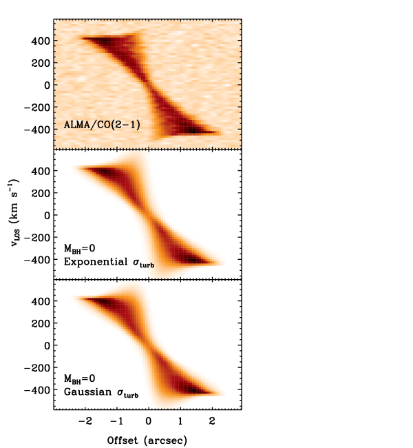
Figure 14.— PVDs for models with the exponential and Gaussian $\sigma_{\mathrm{turb}}$ profiles. Compared with PVDs for the flat $\sigma_{\mathrm{turb}}$ model (Figure 12), these PVDs fit the data much better at large radii in the disk ($r>1\arcsec$) and give much lower $\chi^{2}$ values, but are a poor match to the central velocity upturn.

5.4. Stellar Mass Profile

As a test to assess the sensitivity of $M_{\mathrm{BH}}$ to the inner mass profile of the galaxy, we ran a model fit using the mass profile measured from the HST F814W image with $\Upsilon$ as a free parameter, using the flat $\sigma_{\mathrm{turb}}$ profile. The model converged on a best-fitting mass of $M_{\mathrm{BH}}=9.85\times 10^{8}$ ${M}_{\odot}$ and $\sigma_{\mathrm{turb}}=25.0$ km s^-1, and the stellar mass profile for the best fit is illustrated in Figure 6. The best fit has $\chi^{2}=11690.8$, compared with the value 11171.8 for the best fit using the Rusli et al. (2011) mass profile and flat $\sigma_{\mathrm{turb}}$.

It is reasonable to assume that the stellar luminosity profile measured from $K$-band data is a more accurate representation of the galaxy structure, having less sensitivity to dust extinction, and the $K$-band galaxy profile gives a lower $\chi^{2}$ value for the dynamical model fit. The difference in BH masses measured with the two profiles illustrates the importance of using a mass profile measured from near-IR imaging whenever possible, to minimize the impact of extinction. Higher-resolution kinematic data would also lessen the impact of extinction on the derived $M_{\mathrm{BH}}$; when the central, nearly Keplerian region of the disk is better resolved, the impact of errors in $M_{\star}(r)$ on the derived $M_{\mathrm{BH}}$ will become smaller.

5.5. Fits to the PVD

Another option for model fitting is to carry out fits to the PVD rather than to the full data cube. This may have an advantage in that the PVD describes the major axis kinematics of the disk, and fitting models to the PVD rather than to the full data cube could have better sensitivity to the central velocity upturn and lead to better constraints on $M_{\mathrm{BH}}$. However, fits to the PVD would not be able to constrain the disk inclination, kinematic PA, or centroid position as well as fits to the data cube, and these parameters would need to be constrained or fixed.

We carried out a fit to the PVD using the flat $\sigma_{\mathrm{turb}}$ model, with the values of $i$, $\Gamma$, and the $x$ and $y$ centroid positions fixed to their best-fitting values from the corresponding fit to the full data cube. Free parameters included $M_{\mathrm{BH}}$, $\Upsilon$, $\sigma_{\mathrm{turb}}$, $v_{\mathrm{sys}}$, and $f_{0}$. For each model iteration, we extracted a PVD following the same procedures used on the data, with a four pixel extraction width. For the calculation of $\chi^{2}$, we measured the background noise as the standard deviation of pixel values in blank regions of the PVD. We note that the PVD still exhibits strongly correlated noise among pixels along the position axis over a scale of $\sim 4$ pixels.

This model run gave best-fitting values of $M_{\mathrm{BH}}=6.5\times 10^{8}$ ${M}_{\odot}$, $\Upsilon_{R}=7.18$, and $\sigma_{\mathrm{turb}}=21.6$ km s^-1. Thus, in this case fitting to the PVD rather than to the data cube altered the best-fitting value of $M_{\mathrm{BH}}$ by just 8%. This can be attributed to the fact that the disk is so highly inclined that a 4-pixel wide extraction of the PVD already contains much of the kinematic information of the disk as a whole.

The fits to the full data cube demonstrated that $\chi^{2}$ minimization has a tendency to optimize the model fit to the outer disk, with relatively low sensitivity to the small number of pixels in the central velocity upturn region. We therefore carried out another model run in which $\chi^{2}$ was calculated only over a restricted set of pixels in the PVD corresponding to the spatial and velocity region sensitive to the central upturn. For this model run, we fixed $\Upsilon$ to its best-fitting value from the previous fit to the full PVD, leaving $M_{\mathrm{BH}}$, $\sigma_{\mathrm{turb}}$, $v_{\mathrm{sys}}$, and $f_{0}$ as free parameters. The calculation of $\chi^{2}$ was carried out only for pixels in the PVD corresponding to $r<1\arcsec$ and $v_{\mathrm{LOS}}>300$ km s^-1. This model run gave $M_{\mathrm{BH}}=5.7\times 10^{8}$ ${M}_{\odot}$ and $\sigma_{\mathrm{turb}}=37.7$ km s^-1. As in the case of fitting to the full PVD, fitting models with $\sigma_{\mathrm{turb}}$ restricted to lower values led to higher values of $M_{\mathrm{BH}}$ (but higher $\chi^{2}$): enforcing an upper limit of $\sigma_{\mathrm{turb}}=10$ km s^-1 gave $M_{\mathrm{BH}}=8.0\times 10^{8}$ ${M}_{\odot}$. Since the best-fitting $M_{\mathrm{BH}}$ values were very similar to the values derived from fits to the full data cube, we conclude that for this dataset there is no clear advantage to fitting models to either the full PVD or to the central high-velocity region of the PVD.

5.6. Final Results

The dynamical model fits do not lead to a definitive determination of $M_{\mathrm{BH}}$, primarily because the inferred value of $M_{\mathrm{BH}}$ depends very directly on the specific choice of some parameterized model for $\sigma_{\mathrm{turb}}(r)$ or on any upper limit imposed on the value of $\sigma_{\mathrm{turb}}(r)$. The simplest model, with the flat $\sigma_{\mathrm{turb}}$ profile, converges tightly to $M_{\mathrm{BH}}=6.0\times 10^{8}$ ${M}_{\odot}$. The best-fitting model has $\chi^{2}_{\nu}=4.4$, however, and the line profiles shown in Figure 11 demonstrate that $\chi^{2}$ is dominated by localized regions where the modeled profiles deviate systematically from the data, indicating that the models are failing to capture some essential structure in the disk’s velocity field, turbulent velocity dispersion profile, or surface brightness profile. In the outer disk, the observed line profiles are clearly narrower than the best-fitting overall value of $\sigma_{\mathrm{turb}}=24.7$ km s^-1, but when $\sigma_{\mathrm{turb}}$ is fixed to lower values, the line profiles at intermediate radii in the disk deviate even more strongly from the data (also visible in Figure 11). The central high-velocity envelope of the PVD appears qualitatively to be better matched by a model with $\sigma_{\mathrm{turb}}$ fixed at 10 km s^-1 (implying $M_{\mathrm{BH}}=8\times 10^{8}$ ${M}_{\odot}$) than with $\sigma_{\mathrm{turb}}=24.7$ km s^-1, but the model with $\sigma_{\mathrm{turb}}=10$ km s^-1 is a much worse fit overall in terms of $\chi^{2}$. Restricting the model fit to a small sub-region of the PVD at small radius and high velocity does not alter these results substantially, compared with fits to the full data cube. The systematic deviations between models and data can also be seen in the kinematic moment maps (Figure 3). While the models reproduce the overall structure of the kinematic maps reasonably, even up to $h_{5}$ and $h_{6}$, there are obvious differences in detail, which can plausibly be attributed to an inadequate model for the spatial distribution of $\sigma_{\mathrm{turb}}$ in the disk.

Models in which $\sigma_{\mathrm{turb}}$ is allowed to vary with radius give much lower values of $\chi^{2}_{\nu}$, although still well above unity. Fits carried out with the exponential and Gaussian $\sigma_{\mathrm{turb}}$ profiles drive $M_{\mathrm{BH}}$ to zero, substituting dispersion for rapid rotation in the inner region of the disk. These models are formally more successful than the flat $\sigma_{\mathrm{turb}}$ models because they fit the outer disk much better while matching the inner high-velocity envelope of the PVD relatively poorly. The lowest $\chi^{2}$ value is found for the Gaussian $\sigma_{\mathrm{turb}}$ model fit, which gives $\chi^{2}_{\nu}=2.95$ at $M_{\mathrm{BH}}=0$. The appearance of the PVDs for the exponential and Gaussian $\sigma_{\mathrm{turb}}$ models gives a fairly clear indication that the high central dispersions are spurious, however. These fits imply central values of $\sigma_{\mathrm{turb}}$ that are probably unphysically large (over 250 km s^-1 in the case of the exponential profile), but restricting the maximum $\sigma_{\mathrm{turb}}$ amplitude to lower values produces significantly worse fits with much higher $\chi^{2}$ (Figure 13). With the exponential profile, a limit on the maximum value of $\sigma_{\mathrm{turb}}$ ($<50$ km s^-1) based on observations of resolved GMCs in other environments leads to $M_{\mathrm{BH}}$ in the range $(4-8)\times 10^{8}$ ${M}_{\odot}$.

These difficulties in constraining $M_{\mathrm{BH}}$ appear to be driven by a combination of factors: the models systematically deviate from the data in some locations of the disk by amounts much larger than the observational uncertainties; the beam-smeared line profiles near the disk center are so broad that the model fits are unable to distinguish clearly between rotation and turbulence as the source of the broadening; a relatively small number of data pixels are located in spatial and velocity regions of the data cube that are highly sensitive to $M_{\mathrm{BH}}$; and the S/N in those $M_{\mathrm{BH}}$-sensitive pixels is relatively low.

Fortunately, the disk inclination and orientation parameters, centroid position, and systemic velocity are well constrained by the model fits, and we obtain consistent values for these parameters regardless of the $\sigma_{\mathrm{turb}}$ prescription that is used. The stellar mass-to-light ratio in the best-fitting models is consistent with the value of $\Upsilon_{R}=7.35$ from Rusli et al. (2011). For the models with flat, exponential, and Gaussian $\sigma_{\mathrm{turb}}$, we obtain best-fitting values of $\Upsilon_{R}=7.25$, 7.94, and 7.96, respectively. The two latter cases should be considered effectively as upper limits on $\Upsilon_{R}$, however, since these model fits converged on $M_{\mathrm{BH}}=0$.

The flat and exponential $\sigma_{\mathrm{turb}}$ models together point to a BH mass that is likely to be in the range $\sim(4-8)\times 10^{8}$ ${M}_{\odot}$, under the assumption that a plausible maximum value for $\sigma_{\mathrm{turb}}$ in the inner disk is $\sim 50$ km s^-1. We adopt this as a provisional and preliminary conclusion, but we emphasize that this is not a quantitatively rigorous result. We are unable to derive meaningful confidence limits on $M_{\mathrm{BH}}$ owing to the high $\chi^{2}$ values for our models as well as the fact that the best $\chi^{2}$ values (by far) are found for models with extremely large (and probably spurious) values of $\sigma_{\mathrm{turb}}$ in the inner portion of the disk. With no clear way to determine $\sigma_{\mathrm{turb}}(r)$ independently or to constrain its maximum possible value, a firm lower limit on $M_{\mathrm{BH}}$ cannot be derived from the Cycle 2 data. In all of our models, $\chi^{2}$ rises steeply at $M_{\mathrm{BH}}>10^{9}$ ${M}_{\odot}$; the disk kinematics do not appear to be compatible with the value $M_{\mathrm{BH}}=(1.45\pm 0.20)\times 10^{9}$ ${M}_{\odot}$ found by Rusli et al. (2011).

6. Discussion

The 0$\farcs$3 resolution ALMA observation of NGC 1332 permits an instructive case study for gas-dynamical BH detection. With this dataset, we are working in the regime where the BH sphere of influence may be marginally resolved, in that the central velocity upturn is visible as the upper envelope to the PVD at small radii, but the central high-velocity rotation is badly blurred with low-velocity emission due to beam smearing and the disk’s nearly edge-on inclination. In essence, $r_{\mathrm{g}}$ appears to be nearly resolved along the disk major axis, but it is badly unresolved along the disk’s minor axis. This makes it difficult to derive strong constraints on $M_{\mathrm{BH}}$ from the information contained in the central velocity upturn. The difficulties in modeling the NGC 1332 disk dynamics described here are particularly acute since the disk is very close to edge-on, but we anticipate that these same issues will arise in any situation in which the BH sphere of influence is not well resolved.

6.1. The BH sphere of influence in gas-dynamical measurements

The “radius of influence” for BHs is generally defined as the radius within which the BH is the dominant contribution to the galaxy’s mass profile. In the absence of a mass model for the galaxy, $r_{\mathrm{g}}$ is taken to be the radius within which the circular velocity due to the gravitational potential of the BH rises above the surrounding bulge velocity dispersion $\sigma_{\star}$: $r_{\mathrm{g}}=GM/\sigma_{\star}^{2}$. Since $\sigma_{\star}$ is not spatially constant within a galaxy bulge, and its central value is affected by the BH itself, this definition does not give a uniquely well-defined value of $r_{\mathrm{g}}$, but it does provide a useful general guideline for the radius that should be resolved in order to detect the dynamical effect of the BH. The gravitational influence of the BH can be detected at radii beyond $r_{\mathrm{g}}$, but at progressively larger radii the enclosed mass becomes dominated by stars. Measuring $M_{\mathrm{BH}}$ when $r_{\mathrm{g}}$ is unresolved then becomes an exercise in detecting a small fractional contribution to the total gravitating mass on unresolved spatial scales, and the results can be highly susceptible to systematic errors in determination of the stellar mass profile or in other aspects of the model construction.

The criterion of resolving $r_{\mathrm{g}}$ as the minimal requirement for clear detection of the dynamical effect of the BH ignores one crucial factor, highlighted by the NGC 1332 data. Along the minor axis of an inclined disk, the projected distance from the nucleus to a point at distance $r_{\mathrm{g}}$ from the nucleus is compressed by a factor of $\cos i$. This is an important effect for highly inclined disks: for NGC 1332, $\cos i\approx 0.11$. In an observation just sufficient to resolve $r_{\mathrm{g}}$ along the disk major axis in NGC 1332, $r_{\mathrm{g}}$ along the disk’s projected minor axis would be unresolved by an order of magnitude. In the ALMA data described here, the poor spatial resolution along the disk’s minor axis direction leads directly to severe beam smearing, causing the line profiles to be dominated by low-velocity emission even at small radii along the disk major axis.

Our examination of the NGC 1332 disk dynamics suggests that for gas-dynamical BH mass measurements, the key criterion for whether the BH sphere of influence is resolved should be whether $r_{\mathrm{g}}$ is resolved along the disk’s projected minor axis, not along its major axis as is usually assumed. In other words, to ensure that the central velocity upturn is clearly resolved and not severely spatially blended with low-velocity emission, the observations should resolve an angular scale corresponding to $r_{\mathrm{g}}\cos i$. For highly inclined disks such as NGC 1332, the requirements on angular resolution for dynamical detection of BHs are thus much more stringent than for disks at moderate inclination angles. BH mass measurements from disks observed at very low inclination angles will present a different set of challenges, and will be particularly difficult if $\sin i$ is so small that that the line-of-sight component of the disk’s rotational velocity is not much larger than the turbulent or random velocities in the disk. All else being equal, gas-dynamical BH mass measurements will require higher velocity resolution for disks of lower inclination, and higher angular resolution for high inclinations.

To what extent is $r_{\mathrm{g}}$ resolved in NGC 1332 with the Cycle 2 ALMA observation? Assuming $M_{\mathrm{BH}}=6\times 10^{8}$ ${M}_{\odot}$ and using $\sigma_{\star}=328$ km s^-1 (Kormendy & Ho, 2013), the kinematic definition of the radius of influence gives $r_{g}=24$ pc. This is equivalent to an angular radius of 0$\farcs$22, indicating that the BH radius of influence along the disk major axis would be slightly unresolved. In contrast, $r_{g}\cos i=0\farcs 027$, so the radius of influence is unresolved by an order of magnitude in the minor-axis direction. We can also use the dynamical modeling results to estimate the size of $r_{\mathrm{g}}$ as the radius of the sphere within which $M_{\star}(r)=M_{\mathrm{BH}}$. For $M_{\mathrm{BH}}=6.0\times 10^{8}$ ${M}_{\odot}$, our best-fitting model with the flat $\sigma_{\mathrm{turb}}$ profile also gives $r_{\mathrm{g}}=24$ pc, so the two definitions of $r_{\mathrm{g}}$ give identical results in this case. For the model having $\sigma_{\mathrm{turb}}=10$ km s^-1 and $M_{\mathrm{BH}}=8\times 10^{8}$ ${M}_{\odot}$, $r_{\mathrm{g}}$ is slightly larger at 29.5 pc or 0$\farcs$27 along the disk major axis, similar to the 0$\farcs$27 resolution of the ALMA data. The stellar-dynamical value of $M_{\mathrm{BH}}=1.45\times 10^{9}$ ${M}_{\odot}$ from Rusli et al. (2011) implies a larger sphere of influence, $r_{\mathrm{g}}=58$ pc or 0$\farcs$54.

Figure 15 illustrates the severity of the beam-smearing effect for the NGC 1332 data. This figure presents the modeled circular velocity curve $v_{\mathrm{circ}}(r)$ for the best-fitting model having flat $\sigma_{\mathrm{turb}}$ and $M_{\mathrm{BH}}=6.0\times 10^{8}$ km s^-1, including curves showing $v_{\mathrm{circ}}(r)$ due to the BH alone, the stars alone, and the combined gravitational potential of the BH and stars. For comparison with the data, we take the $k_{1}(r)$ profile from kinemetry and divide by $\sin i$ to produce an observed profile of mean rotation velocity along the disk major axis, and we also display the $k_{1}(r)$ profile measured from a kinemetry fit to the $v_{\mathrm{LOS}}$ map of the dynamical model. (With $i\approx 83\arcdeg$, $\sin i$ is so close to unity that it can be essentially ignored.) In the limit of extremely high angular resolution, the $k_{1}$ curve would closely follow the curve of $v_{\mathrm{circ}}$ for the combined mass profile of the BH and stars. As a consequence of beam smearing and the high disk inclination, the observed line-of-sight centroid velocity $k_{1}$ falls far below the actual major-axis $v_{\mathrm{circ}}$ profile at nearly all radii in the disk, even at radii significantly larger than one resolution element from the galaxy nucleus. One might naively expect that $k_{1}$ would closely track $v_{\mathrm{circ}}$ from large radii down to approximately the resolution limit of the data, but in fact $k_{1}$ begins to deviate below $v_{\mathrm{circ}}$ at a radius roughly five times larger than the angular resolution limit.

This analysis further reinforces the conclusion that, although $r_{\mathrm{g}}$ is likely to be nearly resolved along the disk’s major axis, the mean or centroid velocities measured at locations along the disk major axis have essentially no sensitivity to $M_{\mathrm{BH}}$. When the information about $M_{\mathrm{BH}}$ is contained primarily in the shapes of the beam-smeared line profiles rather than in the centroid velocity $v_{\mathrm{LOS}}$ measured from the line profile at each position, it becomes extremely challenging to derive accurate constraints on $M_{\mathrm{BH}}$.

For our fiducial mass model displayed in Figure 15, the presence of emission out to $\pm 500$ km s^-1 from the systemic velocity (as observed in the PVD) implies that the disk emission extends down to $r\approx 15$ pc, well inside $r_{\mathrm{g}}$ (provided that this outermost velocity is primarily the result of rotation rather than turbulence). The upper limit to the observed rotation speed could be due to the presence of a “hole” in the molecular disk at $r<15$ pc, or simply from a central surface brightness at $r<15$ pc too low to detect in this observation. This scale is well inside the $r\approx 29$ pc angular resolution of our data.

Figure 15.— Plot of circular velocity $v_{\mathrm{circ}}$ as a function of radius, to illustrate the impact of beam smearing on the major axis velocity profile. Model profiles are calculated for the best-fitting model with $M_{\mathrm{BH}}=6.0\times 10^{8}$ ${M}_{\odot}$ and $\sigma_{\mathrm{turb}}=24.7$ km s^-1. Dotted Curve: $v_{\mathrm{circ}}(r)$ for the BH alone. Short-dashed curve: $v_{\mathrm{circ}}(r)$ for the host galaxy stellar mass alone. Solid curve: $v_{\mathrm{circ}}(r)$ for the combined profile of the BH and stars. Long-dashed curve: The major-axis velocity profile $k_{1}/\sin(i)$ measured from the observed ALMA $v_{\mathrm{LOS}}$ map using kinemetry, where $\sin(i)=0.994$. Dot-dashed curve: Kinemetry profile of $k_{1}/\sin(i)$ measured from the $v_{\mathrm{LOS}}$ map of the model, which closely follows that of the data. The dotted vertical line gives the radius corresponding to the resolution limit of the ALMA data ($\theta$), and the solid vertical line denotes $r_{g}$ for $M_{\mathrm{BH}}=6.0\times 10^{8}$ ${M}_{\odot}$. Beam smearing and the disk’s high inclination result in an observed major-axis velocity curve that falls far below the disk’s circular velocity at nearly all radii in the disk.

Davis (2014) proposed a new figure of merit for gas-dynamical BH mass measurements as an alternative to the criterion of resolving $r_{\mathrm{g}}$ for planning future observations. This approach defines $v_{\mathrm{obs}}(r)$ as the line-of-sight rotation velocity of a parcel of gas at some radius $r$ in a galaxy, and $v_{\mathrm{gal}}(r)$ as the rotation speed that parcel would have in the absence of a central BH (which can be determined from $M_{\star}(r)$, accounting for uncertainty in $\Upsilon$). The figure of merit $\Gamma_{\mathrm{FOM}}$ is defined in terms of the confidence level at which $v_{\mathrm{obs}}$ can be distinguished from $v_{\mathrm{gal}}\sin i$ using spatially resolved observations of disk kinematics, if the uncertainty in measured velocity at a given location is $\delta v$. The appropriate distance $r$ to compute this figure of merit is described as the smallest resolvable distance from the galaxy center, corresponding to the telescope’s beam size, since this is the radius within which the BH mass is most dominant in the data.

Our NGC 1332 data highlight a particular issue with this figure of merit definition. Along the disk major axis at a distance of one resolution element from the center in NGC 1332, beam smearing and rotational broadening make the observed line profiles extremely broad and asymmetric, breaking the one-to-one correspondence between position and line-of-sight rotation velocity that would be observed in data of much higher angular resolution. If $v_{\mathrm{obs}}(r)$ is identified with the mean or centroid of the line-of-sight velocity profile, it will be subject to the beam-smearing effect illustrated in Figure 15, in which case $v_{\mathrm{obs}}(r)$ can deviate strongly from the disk’s intrinsic $v\sin i$ out to radial scales significantly larger than the angular resolution of the observations. The definition of $\Gamma_{\mathrm{FOM}}$ does not account for the confounding effects of beam smearing and disk inclination on the line profiles, an effect that becomes increasingly important at higher disk inclinations. Using the $\Gamma_{\mathrm{FOM}}$ criterion, Davis (2014) argues that BH masses can be determined even when the observational resolution is $\sim 2$ times larger than the angular size of $r_{\mathrm{g}}$. We suggest that observations with such low resolution would not generally have the power to constrain $M_{\mathrm{BH}}$ accurately.

We propose that the best criterion to plan future observations is simply whether $r_{\mathrm{g}}$ is resolved along the disk’s projected minor axis for the anticipated value of $M_{\mathrm{BH}}$. The ideal situation is one in which the observations provide several independent resolution elements across $r_{\mathrm{g}}$, even along the minor axis of the disk. Such high resolution observations will have the capability to fully lift degeneracies between $M_{\mathrm{BH}}$, $\Upsilon$, and $\sigma_{\mathrm{turb}}$, and yield highly accurate (and precise) measurements of $M_{\mathrm{BH}}$. Deriving a more rigorous figure of merit criterion for gas-dynamical BH detection would require a comprehensive suite of simulations incorporating beam smearing, to test the impact of angular resolution, disk inclination, S/N, and other parameters on the accuracy of BH mass determination.

6.2. Model fitting methods and sources of error

In past gas-dynamical measurements of BH masses using HST data, models were fit to quantities measured from the data, specifically to the line-of-sight velocity at each spatial pixel, and sometimes to the line-of-sight velocity dispersion as well. This is a relatively time-consuming technique, because it requires measurements of $v_{\mathrm{LOS}}$ and $\sigma_{\mathrm{LOS}}$ at each point in the modeled velocity field for each model realization so that the models and data can be compared. In principle, the modeled emission-line profiles could be compared directly with the data instead of going through the intermediate step of measuring kinematic moments from each model iteration. However, despite some initial attempts (Bertola et al., 1998; Barth et al., 2001a), direct fitting of modeled line profiles has not proved to be a successful approach for BH mass measurements based on optical emission-line data. Obstacles to direct line-profile fitting for optical data include the blending of multiple emission lines such as H$\alpha$ and the [N II] $\lambda\lambda 6548,6583$ lines, the presence of broad emission-line components blended with the resolved narrow-line emission, and the difficulty of measuring or modeling the emission-line surface brightness profile to sufficiently high accuracy for direct line-profile fitting to succeed.

The ALMA data, on the other hand, are much more amenable to direct fitting of models to the observed data cube. Fitting models to the data cube makes use of all available information in the data and should therefore be preferred whenever it is feasible. We found that for this dataset, fitting to the PVD (either in whole or over restricted regions) did not lead to substantial changes in the inferred $M_{\mathrm{BH}}$, compared with fitting to the full information in the data cube. Furthermore, fitting models directly to the data cube is the most efficient approach, in that it avoids the additional steps of extracting a PVD or kinematic moment maps from each individual realization of a modeled data cube for a particular parameter set.

Gas-dynamical model fits can lead to very high-precision constraints on $M_{\mathrm{BH}}$, as discussed by Gould (2013). However, in the regime of very precise model fitting results, it becomes very important to explore potential systematic uncertainties that might affect the measurement, including uncertainty in the slope or shape of the extended mass profile and uncertainty in the turbulent velocity dispersion profile. These problems are compounded when the BH’s sphere of influence is not well resolved, or when models are fitted to a spatial region in which most pixels are at locations well outside of $r_{\mathrm{g}}$. Neglecting these systematics could lead to catastrophic errors in determining $M_{\mathrm{BH}}$– that is, errors far larger than the formal model-fitting uncertainties. The ideal situation is one in which the data quality (resolution and S/N) are sufficient to allow model parameters to be constrained by fitting models only to spatial regions within $r<r_{\mathrm{g}}$, the region in which the kinematics are maximally sensitive to $M_{\mathrm{BH}}$.

In this work, we have focused on modeling uncertainties due to the degeneracy between rotation and turbulent motion, since this problem is particularly severe at high disk inclination; in other cases, uncertainty in the stellar mass profile may be the dominant contribution to the error budget. Often, in gas-dynamical model fitting, the stellar luminosity profile is taken to be a fixed profile, with just a single scaling factor $\Upsilon$ as a free parameter. This procedure is, however, prone to underestimate the uncertainty in $M_{\mathrm{BH}}$, because model fits can converge tightly on a best-fitting value of $M_{\mathrm{BH}}$ even if the measured stellar luminosity profile deviates from the actual extended mass profile of the galaxy. When $r_{\mathrm{g}}$ is not well resolved, it is particularly important to incorporate a realistic level of uncertainty in the slope or shape of the deprojected stellar luminosity profile into the model fitting process. We have not explored this uncertainty in detail in this work, but our simple experiment of measuring $M_{\mathrm{BH}}$ using the galaxy profile measured from the HST F814W image illustrates the nature of the problem. For molecular gas-dynamical $M_{\mathrm{BH}}$ measurements, the central light profile of the host galaxy will most often be severely impacted by dust absorption, and extinction may still be an issue even in the $K$ band, as illustrated by the VLT SINFONI image of NGC 1332 from Rusli et al. (2011). This problem can be alleviated to some extent by masking out the most heavily obscured regions of the disk when measuring the stellar luminosity profile, or by using multi-color data to model and remove the effects of extinction.

Additionally, radial gradients in the stellar mass-to-light ratio, if present, would lead to errors in inferring $M_{\star}(r)$ from the galaxy’s light profile. The impact of $\Upsilon$ gradients on stellar-dynamical measurements has been investigated by McConnell et al. (2013), who found that plausible $\Upsilon$ gradients could bias BH mass measurements in elliptical galaxies by $\sim 20-30\%$. The influence of $\Upsilon$ gradients on gas-dynamical measurements should be less severe since gas-dynamical data only samples the stellar mass profile within the region enclosed by the disk’s radius, but past gas-dynamical work has not directly tested or simulated the contribution of $\Upsilon$ gradients to uncertainty on $M_{\mathrm{BH}}$. The best and most secure approach to circumvent these difficulties is to obtain kinematic data that highly resolve $r_{\mathrm{g}}$, so that $M_{\star}(r)$ is much smaller than $M_{\mathrm{BH}}$ over the innermost resolution elements of the data. Then, uncertainty in the stellar mass profile will not have a large impact on $M_{\mathrm{BH}}$.

Another potential source of systematic error in the model fits is the CO surface brightness map. Beam smearing (both in the data and the models) mixes information on rotation velocity, turbulent linewidth, and surface brightness near the disk center, and errors in the assumed surface brightness map can lead directly to errors in $M_{\mathrm{BH}}$. The high inclination of the NGC 1332 disk makes it much more difficult to discern any surface brightness substructure that may be present. In general, resolving the emission-line surface brightness structure on small radial scales is a key requirement for accurate modeling, along with resolving the kinematic structure. Ideally, the disk’s surface brightness profile should be resolved on scales of $r_{\mathrm{g}}\cos i$ or smaller. Given the other large sources of systematic uncertainty in modeling the NGC 1332 data, we have not explored the impact of surface brightness errors on our model fits, but unresolved surface brightness substructure could be responsible for a portion of the high $\chi^{2}$ values we obtain.

As noted by Gould (2013), it is also the case that distance uncertainty contributes directly to uncertainty in $M_{\mathrm{BH}}$, because the value of $M_{\mathrm{BH}}$ inferred from dynamical modeling scales linearly with the assumed distance. Most BH mass measurements have not incorporated distance uncertainties into their error analysis, but this should be borne in mind in situations where the formal model-fitting precision on $M_{\mathrm{BH}}$ is so high that distance uncertainty becomes a major component of the error budget on $M_{\mathrm{BH}}$. For NGC 1332, recent distance measurements listed in the NASA/IPAC Extragalactic Database (NED) are between 21.9 and 24.6 Mpc (Kundu & Whitmore, 2001; Tully et al., 2013), and the contribution of distance uncertainty to the error budget on $M_{\mathrm{BH}}$ is much smaller than the other sources of systematic uncertainty associated with the dynamical modeling.

6.3. Disk structure

A major issue for gas-dynamical BH mass measurements is the treatment of the turbulent velocity dispersion. The disk’s physical thickness will depend on $\sigma_{\mathrm{turb}}/v_{\mathrm{rot}}$, where $v_{\mathrm{rot}}$ is the disk’s rotational velocity, and if the turbulent velocity dispersion contributes an effective dynamical pressure that supports the disk against gravity, then this must be accounted for in the dynamical modeling. Enclosed mass scales with $v_{\mathrm{rot}}^{2}$ for a dynamically cold disk or $\sigma^{2}$ for a purely dispersion-supported system, or (very roughly) $v_{\mathrm{rot}}^{2}+\sigma^{2}$ if both rotation and random motions provide dynamical support for the disk. Thus, if $(\sigma_{\mathrm{turb}}/v_{\mathrm{rot}})^{2}\ll 1$, then the disk can be treated as dynamically cold. In our model calculations, we have included $\sigma_{\mathrm{turb}}$ merely as an empirical broadening to the emergent CO linewidths from the disk, but we have not ascribed any dynamical importance to $\sigma_{\mathrm{turb}}$. These models effectively assume a dynamically cold, flat disk in which $v_{\mathrm{rot}}=v_{\mathrm{circ}}$.

Figure 16 illustrates the radial variation of $\sigma_{\mathrm{turb}}/v_{\mathrm{circ}}$ for the best-fitting model with the flat $\sigma_{\mathrm{turb}}$ profile having $\sigma_{\mathrm{turb}}=24.7$ km s^-1 and $M_{\mathrm{BH}}=6.0\times 10^{8}$ ${M}_{\odot}$. The maximum value reached by $\sigma_{\mathrm{turb}}/v_{\mathrm{circ}}$ is 0.058, at $r=125$ pc. This is a sufficiently low value to justify the treatment of the disk as thin and dynamically cold.

Figure 16.— Radial profile of $\sigma_{\mathrm{turb}}/v_{\mathrm{circ}}$ for the model with $\sigma_{\mathrm{turb}}=24.7$ km s^-1 and $M_{\mathrm{BH}}=6.0\times 10^{8}$ ${M}_{\odot}$.

In the models with turbulent velocity dispersion gradients, the peak $\sigma_{\mathrm{turb}}$ values are much higher: 268 km s^-1 for the exponential $\sigma_{\mathrm{turb}}$ profile and 100 km s^-1 for the Gaussian profile. For reasons described previously, these high $\sigma_{\mathrm{turb}}$ values are probably spurious, since they fail to reproduce the shape of the PVD at small radii and high velocities. In these models, $\sigma_{\mathrm{turb}}/v_{\mathrm{rot}}$ reaches very high values near the disk center, because with no BH, $v_{\mathrm{rot}}$ goes to zero at very small radii. This would imply that the inner disk becomes very thick and dispersion dominated, and if this were the case our model assumptions would break down badly. While this is an extreme and unlikely scenario, we do not actually have a strong constraint on the maximum value of $\sigma_{\mathrm{turb}}$ in the NGC 1332 disk. A definitive measurement of $\sigma_{\mathrm{turb}}/v_{\mathrm{rot}}$ across the disk can only be done using data of higher angular resolution. For now, we consider the $\sigma_{\mathrm{turb}}/v_{\mathrm{rot}}$ profile shown in Figure 16 to be a reasonable estimate, providing some reassurance that the disk can be modeled as thin and dynamically cold.

Future high-resolution ALMA observations will likely be able to constrain BH masses tightly by resolving kinematics within $r_{\mathrm{g}}$. In the regime of extremely high-precision BH mass measurement with well-controlled systematics, the impact of turbulent pressure support on the derived BH mass might not be negligible in comparison with other sources of error, in which case other approaches such as Jeans equation modeling or application of the asymmetric drift formalism might be necessary.

In this work as in most gas-dynamical BH detections, the disk has been treated as essentially a surface of zero thickness. In a highly inclined disk of nonzero thickness, any line of sight through the disk will pass through regions having different line-of-sight rotation velocities. If the disk were optically thin but geometrically thick, it would be important to model the full line-of-sight velocity profiles through the disk rather than treating the disk as a thin surface. The NGC 1332 molecular disk is likely to be optically thick to CO(2–1) emission, as is generally the case in molecular clouds (e.g., Bolatto et al., 2013), and if it is as thin as suggested by the $\sigma_{\mathrm{turb}}/v_{\mathrm{rot}}$ profile, modeling it as a thin surface should be a reasonable approximation to its structure.

The disk also exhibits a mild kinematic twist that signals the likely presence of a warp, probably similar to the warp in the maser disk of NGC 4258 (Herrnstein et al., 2005). In this first examination of the NGC 1332 disk kinematics, we have not attempted to model the warp, but we plan to explore warped-disk models in future work. One approach to modeling a warped disk is to use a tilted-ring model in which the radial variation of the ring inclination and orientation angles is set by the disk’s measured kinemetry profiles (e.g., Neumayer et al., 2007).

The high values of $\chi^{2}$ found for our best-fitting models, and the systematic deviations between the modeled line profiles and the data (Figure 11) indicate that there are real and important aspects of the NGC 1332 disk structure and/or dynamics that are not incorporated in the models. The largest of these systematic problems are likely to be the inadequacy of our $\sigma_{\mathrm{turb}}$ models and CO surface brightness model, and the fact that the warp is neglected in our dynamical models. It is also possible, however, that there may be real departures from circular rotation in the disk such as $m=2$ perturbations to cloud orbits (e.g., Wong et al., 2004), or localized departures from circular orbits due to star formation or other processes within the disk. The line profiles shown in Figure 11 show that the largest deviations of the models from the data are systematic and roughly symmetric on the blueshifted and redshifted sides of the disk, suggesting that localized random velocity irregularities are not the dominant contribution to the large $\chi^{2}$.

Observations of other transitions from the ¹²CO rotational ladder, as well as ¹³CO lines and lines of other molecular species such as HCN and HCO⁺, can provide much more information on the temperature and density conditions in ETG disks (e.g., Crocker et al., 2012; Bayet et al., 2013), and disks such as the one in NGC 1332 will be important targets for further ALMA observations. Additionally, it would be interesting to compare the kinematics and turbulent velocity dispersion profile of the molecular gas with the kinematics of ionized gas on the same angular scales. This can be done with HST STIS observations of the H$\alpha$+[N II] spectral region or other optical lines, or with adaptive optics observations in cases where Br$\gamma$, [Fe II], or other near-infrared lines are strong enough to enable kinematic mapping. Direct comparisons of BH mass measurements using ionized and molecular gas dynamics in the same galaxy would be worth pursuing as well, to test whether molecular gas is indeed a more accurate tracer of circular velocity than ionized gas within the close environments of supermassive BHs.

6.4. Comparison with previous $M_{\mathrm{BH}}$ measurements

Since our models do not provide quantitatively satisfactory fits to the ALMA data cube, we cannot compare our results with the previous $M_{\mathrm{BH}}$ measurements from Humphrey et al. (2009) and Rusli et al. (2011) in a rigorous fashion. However, it is clear that models with $M_{\mathrm{BH}}$ in the range found by Rusli et al. (2011), $M_{\mathrm{BH}}=(1.45\pm 0.20)\times 10^{9}$ ${M}_{\odot}$, lead to far higher $\chi^{2}$ values than our best-fitting models. This is the case for all of the $\sigma_{\mathrm{turb}}$ prescriptions that we have examined, so our provisional $M_{\mathrm{BH}}$ estimate appears to be incompatible with their result. The discrepancy is particularly intriguing in that we are using the same stellar mass profile measured by Rusli et al. (2011) for their mass modeling.

The mass model from Rusli et al. (2011) implies a total enclosed mass of $\approx 2.4\times 10^{9}$ ${M}_{\odot}$ within $r=30$ pc, based on their best-fitting BH mass and their stellar mass profile with $\Upsilon_{R}=7.35$. This gives a circular velocity of 580 km s^-1 at $r=30$ pc, much larger than the maximum speed of $\approx 480$ km s^-1 seen in the ALMA PVD at $r=30$ pc. Adopting the $1\sigma$ lower bound to $M_{\mathrm{BH}}$ from Rusli et al. (2011), $1.25\times 10^{9}$ ${M}_{\odot}$, we would obtain $v_{\mathrm{circ}}(30~{}\mathrm{pc})=550$ km s^-1, still much higher than the observed outer envelope to the PVD at this radius. In our model fit with $M_{\mathrm{BH}}$ fixed to $1.45\times 10^{9}$ ${M}_{\odot}$, the mass-to-light ratio converged to a much lower value of $\Upsilon_{R}=6.02$ in order to attempt to fit the disk kinematics at large radii, but still gave a very poor fit, clearly over-predicting the amplitude of the central velocity upturn as seen in the lower panel of Figure 10.

The Humphrey et al. (2009) measurement of $M_{\mathrm{BH}}=0.52_{-0.28}^{+0.41}\times 10^{9}$ ${M}_{\odot}$ was based on constructing a mass model for NGC 1332 using the hydrostatic equilibrium of the X-ray emitting gas as a probe of the gravitational potential. The model includes components describing the stellar mass distribution of the galaxy (based on a combination of 2MASS data at large scales and the HST F814W image at small radii, with the dust disk masked out), the hot gas profile as measured from Chandra observations, the dark matter halo, and the BH. This method requires the presence of an X-ray emitting hot interstellar medium in hydrostatic equilibrium, and to date it has only been applied to a small number of ETGs including NGC 4261, NGC 4472, and NGC 4649 in addition to NGC 1332 (Humphrey et al., 2008, 2009). The X-ray derived BH masses for NGC 4261 and NGC 4649 are in agreement with masses measured for these galaxies from ionized gas dynamics (NGC 4261; Ferrarese et al., 1996) and stellar dynamics (NGC 4649; Shen & Gebhardt, 2010). For NGC 4472, the X-ray hydrostatic equilibrium method gives $0.64_{-0.33}^{+0.61}\times 10^{9}$ ${M}_{\odot}$ (Humphrey et al., 2009) while a stellar-dynamical analysis finds $M_{\mathrm{BH}}=(2.4-2.8)\times 10^{9}$ ${M}_{\odot}$ for model fits that include a dark matter halo (Rusli et al., 2013). A definitive measurement of $M_{\mathrm{BH}}$ in NGC 1332 using higher-resolution ALMA data can provide a critical test of the X-ray and stellar-dynamical results.

As a fast-rotating ETG with a high central stellar velocity dispersion, NGC 1332 bears some similarities to galaxies such as NGC 1277 and NGC 1271 which have been found to contain extremely massive BHs that are outliers falling well above the $M_{\mathrm{BH}}-L_{\mathrm{bulge}}$ correlations of the general population of ETGs (van den Bosch et al., 2012; Walsh et al., 2015a, 2016; Scharwächter et al., 2015). Assuming the BH mass from Rusli et al. (2011) for NGC 1332, Kormendy & Ho (2013) discuss whether the galaxy is an outlier or not relative to the $M_{\mathrm{BH}}-M_{\mathrm{bulge}}$ relationship. The answer hinges on whether NGC 1332 is treated as a flattened, single-component elliptical galaxy, or a two-component S0 with bulge and disk. If it is a two-component bulge+disk system in which the elongated portion of the galaxy is considered to be a disk component, then the BH would be moderately over-massive relative to its small bulge, but if the galaxy is instead a flattened elliptical with a dominant bulge component accounting for the majority of the light, then the BH–bulge mass ratio is within the normal range for ellipticals. Kormendy & Ho (2013) argue that NGC 1332 is a highly flattened elliptical, in which essentially all of the light can be ascribed to the bulge component. Savorgnan & Graham (2016) also support the bulge-dominated interpretation. If the BH mass is close to our provisional estimate and the value determined by Humphrey et al. (2009), then the galaxy would lie closer to the normal BH–bulge mass ratio for ETGs, and it would even fall in the low-mass tail of the scatter distribution in the $M_{\mathrm{BH}}-\sigma$ relation for ETGs (Figure 15 of Kormendy & Ho, 2013).

6.5. Future prospects for BH mass measurements with ALMA

ALMA observations have an exciting potential for enabling gas-dynamical BH mass measurements, but it remains to be seen how widely applicable this method will be for exploring BH demographics. For ETGs, the available pool of targets for precision measurement of $M_{\mathrm{BH}}$ will be a small fraction of the overall population of ETGs. Well-defined circumnuclear dust disks are only seen in $\sim 10\%$ of ETGs. Measuring accurate BH masses in these galaxies will be most successful when (a) the gas kinematics are dominated by simple disklike rotation, (b) ALMA observations can resolve $r_{\mathrm{g}}\cos i$, and (c) the molecular emission-line surface brightness is high enough that the gas kinematics can be mapped on scales well within $r_{\mathrm{g}}$. This last requirement could prove to be a major limiting factor for ALMA measurements of BH masses; it is not yet known what fraction of circumnuclear disks will have detectable emission extending inward to $r<r_{\mathrm{g}}$. In NGC 1332, the high-velocity emission provides evidence that the disk extends inward to at least $r\approx 15$ pc. However, if there had been a central “hole” in the molecular disk with a radius much larger than $\sim 25$ pc then there would be no high-velocity upturn in the data and accurate measurement of the BH mass would not be possible even with higher resolution observations. Molecular clouds may be easily disrupted in the immediate environments of massive BHs as a result of the extreme shear (Utomo et al., 2015) or due to winds or irradiation from intermittent accretion-powered nuclear activity. Tidal disruption of molecular clouds in the close environments of supermassive BHs has also been suggested as an explanation for the lack of young stellar populations seen in the innermost few parsecs of typical S0 and early-type spiral galaxies (Sarzi et al., 2005). As ALMA observes larger numbers of ETGs having circumnuclear disks, it will be possible to determine the inner structures of these objects and search for any connections with BH mass, nuclear activity level, or other properties.

Accurate measurements of host galaxy luminosity profiles in the near-infrared will be a critically important component of future gas-dynamical $M_{\mathrm{BH}}$ measurements. Ideally, these observations should have angular resolution at least as high as the ALMA data, and next-generation extremely large telescopes equipped with adaptive optics will bring greatly improved capabilities for these measurements.

Several targets for $M_{\mathrm{BH}}$ measurement have already been observed by ALMA in Cycles 0–2, and additional programs have been approved for Cycle 3, so the number of galaxies with detections of high-velocity rotation within $r_{\mathrm{g}}$ should begin to increase rapidly in the near future. The most efficient way to pursue BH mass measurements with ALMA will be to continue carrying out initial, quick observations of galaxies with resolution just sufficient to test for the presence of rapidly rotating gas within $r_{\mathrm{g}}$. Finding evidence of high-velocity rotation within $r_{\mathrm{g}}$ will then justify deeper and higher-resolution observations that can potentially provide exquisite sampling of the gas kinematics within $r_{\mathrm{g}}$. Galaxies for which $M_{\mathrm{BH}}$ can be measured to high accuracy using data that highly resolve $r_{\mathrm{g}}$ are extremely valuable, providing firm anchors to local BH demographics and the BH-host galaxy correlations, in addition to providing strong evidence that the central massive objects are indeed likely to be supermassive BHs (Maoz, 1998).

In our ALMA programs, we are selecting ETG targets based on the presence of well-defined circumnuclear dust disks, which give morphological evidence for dense gas in rotation about the galaxy center. ALMA will likely be an important tool for gas-dynamical detection of BHs in spiral galaxies as well, but it is not yet known what fraction of spiral galaxies contain molecular gas in clean disk-like rotation on scales of $r<r_{\mathrm{g}}$. The dust-disk selection method we have used to identify ETG targets for ALMA would not be applicable to spirals, which typically have more complex, filamentary, or spiral dust-lane structure (e.g., Martini et al., 2003), but the growing number of high-resolution ALMA observations of nearby spirals will make it possible to examine molecular gas kinematics in galaxy nuclei in far greater detail than has previously been possible. Recently, Onishi et al. (2015) presented dynamical modeling of ALMA HCN and HCO⁺ kinematics in the SBb galaxy NGC 1097, deriving a BH mass of $1.40_{-0.32}^{+0.27}\times 10^{8}$ ${M}_{\odot}$. We note that for a stellar velocity dispersion of 196 km s^-1 (Lewis & Eracleous, 2006), the gravitational radius of influence of the NGC 1097 BH would be 15.6 pc or 0$\farcs$22, while the Cycle 0 data used by Onishi et al. (2015) had a beamsize of $1\farcs 6\times 2\farcs 2$. This is an order of magnitude too coarse to resolve $r_{\mathrm{g}}$, and the observed PVD does not show any hint of a central velocity upturn. However, the ALMA PVD does exhibit velocity structure consistent with regular rotation within the inner $r<10\arcsec$, an encouraging sign that higher-resolution observations would have the capability to measure $M_{\mathrm{BH}}$ accurately if the disk kinematics continue to be dominated by regular rotation down to scales within $r_{\mathrm{g}}$.

7. Conclusions

This paper presents an ALMA CO(2-1) observation of the center of NGC 1332 at 0$\farcs$3 resolution. We find evidence for a disk in orderly rotation with evidence for a mild kinematic twist, and a central upturn in maximum line-of-sight velocity consistent with the expected signature of rapid rotation around a compact central mass. Although the quality of the Cycle 2 ALMA data is excellent and the central upturn in maximum rotation speed provides evidence for a compact central mass in NGC 1332, the value of the BH mass cannot be tightly constrained due to severe degeneracies between $M_{\mathrm{BH}}$ and other parameters. These degeneracies stem primarily from beam smearing and rotational broadening of the line profiles, because the BH sphere of influence is slightly unresolved along the disk major axis and very unresolved along the minor axis. We find that the BH mass is degenerate with the turbulent velocity dispersion profile of the disk. Any chosen prescription for the functional form of the disk’s turbulent velocity dispersion profile can lead to formally tight constraints on the BH mass, but different choices for how to model the turbulent velocity dispersion can lead to widely divergent conclusions for the value of the BH mass.

While we are unable to constrain $M_{\mathrm{BH}}$ definitively with the present ALMA data, models with a flat or exponentially declining $\sigma_{\mathrm{turb}}(r)$ profile and $\sigma_{\mathrm{turb}}$ limited to values of $\leq 50$ km s^-1 point to a BH mass in the range $\sim(4-8)\times 10^{8}$ ${M}_{\odot}$. The model fits strongly disfavor a BH mass as high as the value determined by Rusli et al. (2011) from stellar-dynamical modeling, $1.45\times 10^{9}$ ${M}_{\odot}$, but agree well with the value obtained from a hydrostatic analysis of X-ray emission from the diffuse interstellar medium (Humphrey et al., 2009).

When the BH sphere of influence is not highly resolved, gas-dynamical model fits can have a tendency towards high-precision formal constraints on $M_{\mathrm{BH}}$ that are not necessarily matched by correspondingly high accuracy, but which simply reflect the specific choices and assumptions made in constructing models. This can potentially result in catastrophic errors in determining $M_{\mathrm{BH}}$ (i.e., errors that are much larger than the uncertainties in $M_{\mathrm{BH}}$ derived from the usual $\Delta\chi^{2}$ criteria). To obtain gas-dynamical measurements of $M_{\mathrm{BH}}$ that are both precise and accurate, there is no substitute for observations that highly resolve the BH sphere of influence.

We argue that the appropriate criterion for quantifying the feasibility of carrying out a gas-dynamical mass measurement is whether the BH’s radius of influence is resolved along the disk’s minor axis– in other words, the angular resolution of the observation should be smaller than the angular size of $r_{\mathrm{g}}\cos i$. Observations satisfying this criterion (or better) will resolve both the essential kinematics and the emission-line surface brightness substructure in the BH environment, and will lift the degeneracy seen in this dataset between turbulent and rotational motion in the inner disk. When $r_{\mathrm{g}}\cos i$ is highly unresolved, dynamical models can suffer from potentially large systematic uncertainties in deriving $M_{\mathrm{BH}}$ due to uncertainties in the disk’s $\sigma_{\mathrm{turb}}$ profile and sub-resolution surface brightness structure, and due to errors in measurement of the shape of the galaxy’s spatially extended mass distribution.

This initial observation was designed primarily to test for the presence of high-velocity emission from within $r_{\mathrm{g}}$. ALMA is capable of achieving much higher angular resolution than the 0$\farcs$3 beamsize of these data, and new observations of NGC 1332 at 0$\farcs$04 resolution have been scheduled for ALMA’s Cycle 3. These new observations will enable much more detailed fitting of dynamical models on scales $r<r_{\mathrm{g}}$ along the disk’s major axis, and will nearly or fully resolve $r_{\mathrm{g}}\cos i$ (depending on the value of $M_{\mathrm{BH}}$). We anticipate that the new data will provide firm constraints on $M_{\mathrm{BH}}$, demonstrating the full potential of ALMA for dynamical measurement of BH masses.

References

- Alatalo et al. (2013) Alatalo, K., Davis, T. A., Bureau, M., et al. 2013, MNRAS, 432, 1796
- ALMA Partnership et al. (2015) ALMA Partnership, Fomalont, E. B., Vlahakis, C., et al. 2015, ApJ, 808, L1
- Barth et al. (2001a) Barth, A. J., Sarzi, M., Ho, L. C., et al. 2001a, in The Central Kiloparsec of Starbursts and AGN: The La Palma Connection (ASP Conference Series Vol. 249), 370
- Barth et al. (2001b) Barth, A. J., Sarzi, M., Rix, H.-W., et al. 2001b, ApJ, 555, 685
- Bayet et al. (2013) Bayet, E., Bureau, M., Davis, T. A., et al. 2013, MNRAS, 432, 1742
- Bertola et al. (1998) Bertola, F., Cappellari, M., Funes, S. J., José G., et al. 1998, ApJ, 509, L93
- Bolatto et al. (2013) Bolatto, A. D., Wolfire, M., & Leroy, A. K. 2013, ARA&A, 51, 207
- Carilli & Walter (2013) Carilli, C. L., & Walter, F. 2013, ARA&A, 51, 105
- Cappellari (2002) Cappellari, M. 2002, MNRAS, 333, 400
- Crocker et al. (2012) Crocker, A., Krips, M., Bureau, M., et al. 2012, MNRAS, 421, 1298
- da Costa et al. (1991) da Costa, L. N., Pellegrini, P. S., Davis, M., et al. 1991, ApJS, 75, 935
- Davis (2014) Davis, T. A. 2014, MNRAS, 443, 911
- Davis et al. (2013a) Davis, T. A., Alatalo, K., Bureau, M., et al. 2013a, MNRAS, 429, 534
- Davis et al. (2013b) Davis, T. A., Bureau, M., Cappellari, M., Sarzi, M., & Blitz, L. 2013b, Nature, 494, 328
- den Brok et al. (2015) den Brok, M., Seth, A. C., Barth, A. J., et al. 2015, ApJ, 809, 101
- Ferrarese et al. (1996) Ferrarese, L., Ford, H. C., & Jaffe, W. 1996, ApJ, 470, 444
- Gebhardt & Thomas (2009) Gebhardt, K., & Thomas, J. 2009, ApJ, 700, 1690
- Genzel et al. (2000) Genzel, R., Pichon, C., Eckart, A., Gerhard, O. E., & Ott, T. 2000, MNRAS, 317, 348
- Ghez et al. (1998) Ghez, A. M., Klein, B. L., Morris, M., & Becklin, E. E. 1998, ApJ, 509, 678
- Ghez et al. (2008) Ghez, A. M., Salim, S., Weinberg, N. N., et al. 2008, ApJ, 689, 1044
- Gould (2003) Gould, A. 2003, arXiv:astro-ph/0310577
- Gould (2013) Gould, A. 2013, arXiv:1303.0834
- Harms et al. (1994) Harms, R. J., Ford, H. C., Tsvetanov, Z. I., et al. 1994, ApJ, 435, L35
- Herrnstein et al. (2005) Herrnstein, J. R., Moran, J. M., Greenhill, L. J., & Trotter, A. S. 2005, ApJ, 629, 719
- Hicks & Malkan (2008) Hicks, E. K. S., & Malkan, M. A. 2008, ApJS, 174, 31
- Ho et al. (2002) Ho, L. C., Sarzi, M., Rix, H.-W., et al. 2002, PASP, 114, 137
- Hughes et al. (2003) Hughes, M. A., Alonso-Herrero, A., Axon, D., et al. 2003, AJ, 126, 742
- Humphrey et al. (2008) Humphrey, P. J., Buote, D. A., Brighenti, F., Gebhardt, K., & Mathews, W. G. 2008, ApJ, 683, 161
- Humphrey et al. (2009) Humphrey, P. J., Buote, D. A., Brighenti, F., Gebhardt, K., & Mathews, W. G. 2009, ApJ, 703, 1257
- Kormendy & Ho (2013) Kormendy, J., & Ho, L. C. 2013, ARA&A, 51, 511
- Krajnović et al. (2006) Krajnović, D., Cappellari, M., de Zeeuw, P. T., & Copin, Y. 2006, MNRAS, 366, 787
- Krajnović et al. (2008) Krajnović, D., Bacon, R., Cappellari, M., et al. 2008, MNRAS, 390, 93
- Krist et al. (2011) Krist, J. E., Hook, R. N., & Stoehr, F. 2011, Proc. SPIE, 8127, 81270J
- Kundu & Whitmore (2001) Kundu, A., & Whitmore, B. C. 2001, AJ, 122, 1251
- Kuo et al. (2011) Kuo, C. Y., Braatz, J. A., Condon, J. J., et al. 2011, ApJ, 727, 20
- Laine et al. (2003) Laine, S., van der Marel, R. P., Lauer, T. R., et al. 2003, AJ, 125, 478
- Lauer et al. (2005) Lauer, T. R., Faber, S. M., Gebhardt, K., et al. 2005, AJ, 129, 2138
- Leroy et al. (2015) Leroy, A. K., Bolatto, A. D., Ostriker, E. C., et al. 2015, ApJ, 801, 25
- Lewis & Eracleous (2006) Lewis, K. T., & Eracleous, M. 2006, ApJ, 642, 711
- Lucy (1974) Lucy, L. B. 1974, AJ, 79, 745
- Macchetto et al. (1997) Macchetto, F., Marconi, A., Axon, D. J., et al. 1997, ApJ, 489, 579
- Maiolino (2008) Maiolino, R. 2008, New Astronomy Reviews, 52, 339
- Maoz (1998) Maoz, E. 1998, ApJ, 494, L181
- Markwardt (2009) Markwardt, C. B. 2009, Astronomical Data Analysis Software and Systems XVIII, 411, 251
- Martini et al. (2003) Martini, P., Regan, M. W., Mulchaey, J. S., & Pogge, R. W. 2003, ApJS, 146, 353
- Mazzalay et al. (2014) Mazzalay, X., Maciejewski, W., Erwin, P., et al. 2014, MNRAS, 438, 2036
- McConnell et al. (2013) McConnell, N. J., Chen, S.-F. S., Ma, C.-P., et al. 2013, ApJ, 768, L21
- McMullin et al. (2007) McMullin, J. P., Waters, B., Schiebel, D., Young, W., & Golap, K. 2007, Astronomical Data Analysis Software and Systems XVI, 376, 127
- Miyoshi et al. (1995) Miyoshi, M., Moran, J., Herrnstein, J., et al. 1995, Nature, 373, 127
- Neumayer et al. (2007) Neumayer, N., Cappellari, M., Reunanen, J., et al. 2007, ApJ, 671, 1329
- Noel-Storr et al. (2007) Noel-Storr, J., Baum, S. A., & O’Dea, C. P. 2007, ApJ, 663, 71
- Okuda et al. (2005) Okuda, T., Kohno, K., Iguchi, S., & Nakanishi, K. 2005, ApJ, 620, 673
- Onishi et al. (2015) Onishi, K., Iguchi, S., Sheth, K., & Kohno, K. 2015, ApJ, 806, 39
- Richardson (1972) Richardson, W. H. 1972, Journal of the Optical Society of America (1917-1983), 62, 55
- Rusli et al. (2011) Rusli, S. P., Thomas, J., Erwin, P., et al. 2011, MNRAS, 410, 1223
- Rusli et al. (2013) Rusli, S. P., Thomas, J., Saglia, R. P., et al. 2013, AJ, 146, 45
- Sandstrom et al. (2013) Sandstrom, K. M., Leroy, A. K., Walter, F., et al. 2013, ApJ, 777, 5
- Sarzi et al. (2005) Sarzi, M., Rix, H.-W., Shields, J. C., et al. 2005, ApJ, 628, 169
- Savorgnan & Graham (2016) Savorgnan, G. A. D., & Graham, A. W. 2016, MNRAS, 457, 320
- Scharwächter et al. (2013) Scharwächter, J., McGregor, P. J., Dopita, M. A., & Beck, T. L. 2013, MNRAS, 429, 2315
- Scharwächter et al. (2015) Scharwächter, J., Combes, F., Salomé, P., Sun, M., & Krips, M. 2015, arXiv:1507.02292
- Schlafly & Finkbeiner (2011) Schlafly, E. F., & Finkbeiner, D. P. 2011, ApJ, 737, 103
- Shen & Gebhardt (2010) Shen, J., & Gebhardt, K. 2010, ApJ, 711, 484
- Tran et al. (2001) Tran, H. D., Tsvetanov, Z., Ford, H. C., et al. 2001, AJ, 121, 2928
- Tully et al. (2013) Tully, R. B., Courtois, H. M., Dolphin, A. E., et al. 2013, AJ, 146, 86
- Utomo et al. (2015) Utomo, D., Blitz, L., Davis, T., et al. 2015, ApJ, 803, 16
- van den Bosch & de Zeeuw (2010) van den Bosch, R. C. E., & de Zeeuw, P. T. 2010, MNRAS, 401, 1770
- van den Bosch et al. (2012) van den Bosch, R. C. E., Gebhardt, K., Gültekin, K., et al. 2012, Nature, 491, 729
- van der Marel (1994) van der Marel, R. P. 1994, MNRAS, 270, 271
- van der Marel & van den Bosch (1998) van der Marel, R. P., & van den Bosch, F. C. 1998, AJ, 116, 2220
- van Dokkum & Franx (1995) van Dokkum, P. G., & Franx, M. 1995, AJ, 110, 2027
- Verdoes Kleijn et al. (2006) Verdoes Kleijn, G. A., van der Marel, R. P., & Noel-Storr, J. 2006, AJ, 131, 1961
- Walsh et al. (2008) Walsh, J. L., Barth, A. J., Ho, L. C., et al. 2008, AJ, 136, 1677
- Walsh et al. (2010) Walsh, J. L., Barth, A. J., & Sarzi, M. 2010, ApJ, 721, 762
- Walsh et al. (2013) Walsh, J. L., Barth, A. J., Ho, L. C., & Sarzi, M. 2013, ApJ, 770, 86
- Walsh et al. (2015a) Walsh, J. L., van den Bosch, R. C. E., Gebhardt, K., et al. 2015, ApJ, 808, 183
- Walsh et al. (2016) Walsh, J. L., van den Bosch, R. C. E., Gebhardt, K., et al. 2016, ApJ, 817, 2
- Wong et al. (2004) Wong, T., Blitz, L., & Bosma, A. 2004, ApJ, 605, 183
- Young et al. (2008) Young, L. M., Bureau, M., & Cappellari, M. 2008, ApJ, 676, 317