DECLARATION

I, Mr. Monojit Ghosh, S/o Mr. Monoranjan Ghosh, resident of RN-011, PRL student hostel campus, Thaltej, Ahmedabad 380058, hereby declare that the research work incorporated in the present thesis entitled, “Present Aspects and Future Prospects of Neutrino Mass and Oscillation” is my own work and is original. This work (in part or in full) has not been submitted to any University for the award of a Degree or a Diploma. I have properly acknowledged the material collected from secondary sources wherever required. I solely own the responsibility for the originality of the entire content.

Date:

(Monojit Ghosh)

CERTIFICATE

I feel great pleasure in certifying that the thesis entitled, “Present Aspects and Future Prospects of Neutrino Mass and Oscillation” embodies a record of the results of investigations carried out by Mr. Monojit Ghosh under my guidance. He has completed the following requirements as per Ph.D regulations of the University.
     (a) Course work as per the university rules.
     (b) Residential requirements of the university.
     (c) Regularly submitted six monthly progress reports.
     (d) Presented his work in the departmental committee.
     (e) Published minimum of one research papers in a refereed research journal.
     I am satisfied with the analysis, interpretation of results and conclusions drawn. I recommend the submission of thesis.

Date:

Prof. Srubabati Goswami
(Thesis Supervisor)
Professor, THEPH,
Physical Research Laboratory,
Ahmedabad - 380 009

Countersigned by
Head of the Department

I want to take this opportunity to express my sincere and deep gratitude to my supervisor Prof. Srubabati Goswami, for her invaluable guidance, support and involvement throughout my work. Her immense knowledge, perspective and expertise in the subject have helped me during my research and writing of the thesis. Discussing physics with her was fun. We had a great compatibility in understanding the views of each other. She always encouraged me to have a deep and critical understanding of the subject. Due to her friendly nature I could discuss any of my problems with her and she was always there to help me. Her continuous encouragement and motivation gave me confidence to continue research in this field. I could not have imagined having a better advisor for my Ph.D study.

I would specially like to thank Dr. Bijaya Sahoo, Prof. Hiranmaya Mishra, Prof. Jitesh Bhatt, Dr. Namit Mahajan, Dr. Partha Konar, Prof. Raghavan Rangarajan and Prof. Subhendra Mohanty for taking courses on quantum mechanics, particle physics, quantum field theory and mathematical methods. My special thanks goes to my thesis expert Prof. S. Mohanty and the academic committee for reviewing my work thoroughly. I also thank Prof. Amol Dighe, Prof. Raj Gandhi, Prof. Sandhya Choubey, Dr. Sanjib Agarwala and Prof. Uma Shankar for various physics discussions. I would also like to thank Prof J.W.F. Valle for giving me the opportunity to visit IFIC, Valencia. I thank him and Prof. Mariam Tortolla for very useful discussions at IFIC.

I specially thank Dr. Shivani Gupta with whom I have carried out my first research project. I learned a lot of things from her during my initial days of research. I offer my heartiest thanks to Dr. Pomita Ghoshal and Dr. Sushant Raut whose contributions have shaped my knowledge and understanding of neutrino oscillation physics. I thank them for answering my infinite number of questions with patience. I can never forget those long stimulating discussion sessions in my supervisor’s office. I also want to thank Animesh Chatterjee, Moon Moon Devi and Reetanjali Moharana with whom I have spent sleepless nights to finish our project at WHEPP 2013. It has been a nice experience to work with all of you.

I thank my senior Subrata da, my batch mate Gulab and my juniors Chandan Gupta, Chandan Hati, Newton and Vishnu for various useful discussions. I also want to express my gratitude to Abhay, Kuldeep Suthar, Tanmoy Mondal and Ujjal with whom I shared my office space at PRL. They helped me greatly in my research work. A special thanks to Ujjal for a thorough proofreading of my thesis.

My stay at PRL hostel will be memorable due to the presence of all the students including all my seniors, juniors, project associates, project students and my batchmates. The festival celebrations, the sports events, our hundred kilometer long bike trips, hangouts, mind boggling discussions on cinema, politics, literature and many other things will remain unforgettable and will stay close to my heart throughout my life. I want thank you all: Aadhi, Anjali, Arko, Avdhesh, Bhavya, Damu, Dillip, Dinesh, Gaurav Tomar, Girish Chakravarty, Lata, Lekshmy, Midhun, Naveen, Nigam, Priyanka, Reddy, Tanmoy Chattopadhay, Upendra, Wageesh, Yashpal, Abhishek da, Akhilesh, Amrendra, Amzad da, Aravind Saxena, Aravind Thakur, Arun Awasthi, Asish, Bhaswar da, Chinmay da, Fazlul da, Ketan, Koushik da, Moumita di, Pankaj, Prashant, Rabiul da, Shashi, Siddhartha da, Soumya, Srinu, Suman da, Sunil, Sushanta, Tanushree di, Tapas da, Vimal, Vineet, Zeen, Ananta, Gaveshna, Ila, Mansi, Nabyendu da, Ranjita, Shweta, Sudip da, Alok, Anirban, Arun Pandey, Chitrabhanu, Gaurav Jaiswal, Girish Kumar, Guru, Ikshu, Manu, Sanjay, Shradha, Apurv, Ashim, Bivin, Deepak, Dipti, Jiniya, Lalit, Pankaj, Rahul, Sukanya, Venky, Ali, Jabir, Kuldeep Pandey, Kumar, Navpreet, Prahlad, Rukmani, Rupa, Satish, Wriju, Balaji, Bose, Dharak, Ejaz, Jayesh Khunt, Nitesh, Ranjit, Rishi, Santosh, Sharad, Sneha, Subha Anand, Vijayan, Abhishek, Ankur, Dipanweeta, Jayesh Agarwal, Rashika, Ria, Sameer, Sudha and Vasu for spending such beautiful times with me.

I am grateful to all the PRL library, computer center, dispensary and administration staff and also to the staff members of Theoretical Physics Division of PRL for their sincere support.

I also acknowledge Biswajit, Dipankar, Kamakhya, Sabyasachi, Suprabh and Tuhin whom I met in different conferences and became very good friends. We discussed physics whenever we meet and spent precious time together. I could not forget the warm hospitality of Biswajit when we went for the DAE 2014 meeting.

I would also like to thank few of my university friends Anupam, Arghya, Barun, Kalpana, Koushik, Soubhik, Sudip and Suman who frequently keep on asking that how my work is going on and supported me in difficult times. I also want to thank few of my school friends Sandipan, Subho and Tamoghna who were always there to greet me whenever I went home.

I express my deepest gratitude to my family: my parents and my brother for supporting me throughout and for their unconditional love. They always stood beside and encouraged me to pursue a career that I like. This thesis would never be possible without their constant support.

And last but not the least I would also like to thank Anushmita, for proof reading of my thesis partially and motivating me by the following Hemingway’s advice on writing at the time when I was struggling to write my thesis by thinking if a 10 page paper takes several months to write then how it will be possible to manage a thesis consisting of 200 pages:

“Advice on how to write? Sit on a typewriter and start typing. That’s the easiest and the hardest part.”

Monojit

Neutrinos are neutral, spin-$\frac{1}{2}$ particles which undergo only weak interactions. The experimentally observed phenomenon of neutrino oscillation establishes the fact that neutrinos are massive and there is mixing between different neutrino flavours. This constitutes the first unambiguous hint towards the physics Beyond Standard Model (BSM). In the BSM theories, the neutrino mass terms in the Lagrangian lead to the non-diagonal neutrino mass matrix in the flavour basis which depends on neutrino mass and mixing parameters. Thus knowledge of the neutrino oscillation parameters and understanding the underlying symmetries of the neutrino mass matrix are very important as they can give an insight to the new physics beyond Standard Model. Therefore the measurement of different oscillation parameters and studying the structure of the neutrino mass matrix are some of the main goals in neutrino physics at present.

Currently the paradigm of neutrino oscillation between three flavours is well established from different experiments and the oscillation parameters are getting measured with continued precision. The current unknowns in the neutrino oscillation physics in the standard three generation framework are: the neutrino mass hierarchy, octant of $\theta_{23}$ and the leptonic phase $\delta_{CP}$. There are many ongoing/future experiments where these unknown oscillation parameters can be probed. These experiments utilize different sources and detectors as well as different baselines along which oscillations can develop. As the oscillation probabilities depend differently on the parameters in different oscillation experiments, combination of different experiments can often be useful. Apart from three flavours oscillations there are also evidences of oscillation involving sterile neutrinos. In the presence of a sterile neutrino there will be new mixing angles and phases contributing to the oscillation of the neutrinos. This gives rise to the possibility that the well understood phenomenological behaviour of the neutrino mass matrix may change in the presence of sterile neutrinos.

In this thesis we have studied the potential of present/future neutrino oscillation experiments and synergy between them to determine the unknown parameters in the neutrino sector in the light of current experimental results. We consider the beam based experiments T2K, NO$\nu$A, LBNO, LBNE, the atmospheric experiment INO@ICAL and the ultra high energy neutrino experiment IceCube for our analysis. We find that the data from atmospheric neutrino experiment ICAL can significantly improve the CP sensitivity of the long-baseline experiments T2K/NO$\nu$A in their unfavourable parameter space. To improve the sensitivity beyond what can be achieved in T2K/NO$\nu$A, it is important to study the physics potential of the proposed long-baseline experiments LBNO and LBNE in view of the current experiments. We have shown that the required exposure of LBNO and LBNE in determining neutrino mass hierarchy, octant of $\theta_{23}$ and $\delta_{CP}$ can be reduced significantly when data from T2K, NO$\nu$A and ICAL are added to them. We have also explored the possibility to constrain the CP phase $\delta_{CP}$ by analyzing the IceCube data in terms of the flavour compositions of the ultra high energy neutrinos.

We have also studied the phenomenological consequences of texture zeros in the neutrino mass matrices in the presence of a sterile neutrino. We have carried out a detailed analysis of the two-zero and one-zero textures in the 3+1 scenario which involves three active neutrinos and one sterile neutrino. We find that in the 3+1 picture, conclusions differ significantly as compared to the standard 3 generation case. The allowed two-zero textures in the $3\times 3$ structure are more phenomenologically constrained as compared to the $4\times 4$ structure. The correlations between the different oscillation parameters are also very different when the texture zero conditions between the 3 generation and 3+1 generations are compared.

Keywords : Neutrino Physics, Neutrino Oscillation, Long-Baseline Neutrino Experiments, Atmospheric Neutrino Experiments, Ultra High Energy Neutrinos, Leptonic CP Phase, Neutrino Mass Matrix, Sterile Neutrino, Texture Zero

Chapter 1   Introduction

1.1 The Origin of Neutrinos

The physics of neutrinos started with Pauli’s “Neutrino Hypothesis”, but the origin of neutrinos can be traced back to the late 19th century (1896) when Becquerel discovered radioactivity. In radioactivity, nucleus of an unstable atom loses energy by emitting alpha ($\alpha$) particles, beta ($\beta$) particles and gamma ($\gamma$) rays. As in the mechanism of $\alpha$-particle emission, it was believed that $\beta$-decay is also governed by the two-body process

$$N_{0}(A,Z)\rightarrow N(A,Z+1)+e^{-},$$

and energy of the electron is given by the small differences in masses of the nuclei. However, measurements of the electron energy spectra did not match this expectation. By late 1920 it was confirmed that this emission gives a continuous spectra for the electron. This posed a puzzle since a two-body decay would imply a fixed energy line for the electrons. To overcome this Niels Bohr suggested that the energy in the microworld was conserved only on an average, not on an event-by-event basis. In 1930 Pauli postulated the “Neutrino Hypothesis” to save the principle of conservation of energy in $\beta$-decay. He suggested that the continuum spectra might be due to one more “invisible” light neutral particle involved in the $\beta$-decay. With three particles involved, the electron would be able to take any momentum from zero to the maximum allowed value, the balance being taken care of by the other light “invisible” particle. In 1933 Fermi formulated his theory of $\beta$-decay based on Pauli’s hypothesis. At that time the existence of Pauli’s “invisible” particle was accepted and the name neutrino was coined. It was postulated that all $\beta$-decays were due to the same basic underlying process,

$$n\rightarrow p+e^{-}+\bar{\nu}.$$

To satisfy the conservation of angular momentum, neutrinos must be spin-1/2 particles obeying the Fermi-Dirac Statistics. But this theory was firmly established only in 1953 when Clyde Cowan and Frederick Reines detected this weakly interacting particle experimentally [1, 2]. In their experiment, electron type antineutrinos ($\bar{\nu}_{e}$) coming out of nuclear reactors were detected. Now it is well established that there are three types of neutrinos. In 1962, Leon M. Lederman, Melvin Schwartz and Jack Steinberger showed the existence of the muon neutrino ($\nu_{\mu}$) [3] and the first detection of tau neutrino ($\nu_{\tau}$) interactions was announced in the summer of 2000 by the DONUT collaboration at Fermilab [4].

1.2 Neutrinos in Standard Model

The discoveries of different fundamental particles (including neutrinos) in the middle of the 20th century necessitated the formulation of a basic theory to understand the properties of these particles and how they interact. In the effort to unify the electromagnetic, weak, and strong forces, a theory known as the Standard Model (SM) [5] of particle physics was developed throughout the latter half of the 20th century. The current formulation was finalised in the mid-1970s upon experimental confirmation of the existence of quarks. Mathematically, SM is a non-abelian gauge theory based on the symmetry group $U(1)_{Y}\times SU(2)_{L}\times SU(3)_{c}$. In this model the left handed fermion fields are SU(2) doublets and right-handed fermions are SU(2) singlets:

$Q=\begin{pmatrix}u\\ d\\ \end{pmatrix}_{L}$, $L=\begin{pmatrix}\nu_{e}\\ e\\ \end{pmatrix}_{L}$ and $u_{R}$, $d_{R}$, $e_{R}$.

Here $Q$ and $L$ denote the quark and lepton fields respectively belonging to the first generation. In totality SM has three generations of quarks (first generation : $u$, $d$; second generation: $c$, $s$; third generation: $t$, $b$) and three generations of leptons (first generation : $e$, $\nu_{e}$; second generation: $\mu$, $\nu_{\mu}$; third generation: $\tau$, $\nu_{\tau}$). Each of the six quarks have three $SU(3)$ colour charges: red, green and blue. The $W^{\pm}$ and $Z$ bosons are the mediators of the weak force, photon is the carrier of the electromagnetic force and the strong force is mediated by the gluons. In this model neutrinos interact with the other leptonic fields weakly via the exchange of $W^{\pm}$ and $Z$ bosons. The interactions mediated by the $W^{\pm}$ boson are called charge current (CC) interactions and the interactions mediated by the $Z$ boson are called neutral current (NC) interactions. In SM one can count the number of light neutrino species that have the usual electroweak interactions in the following manner: SM allows $Z$ boson to decay to the invisible $\nu\bar{\nu}$ pairs. This invisible decay width is the difference between the total decay width of $Z$ and the visible decay width of $Z$. Visible decay width of $Z$ boson is referred as the sum of its partial widths of decay into quarks and charged leptons. From the LEP (Large Electron-Positron collider) data, the ratio of the invisible decay width of $Z$ and the decay width of $Z$ to the charged leptons ($\Gamma_{{\rm inv}}/\Gamma_{ll}$) is measured as $5.943\pm 0.016$. The SM value for the ratio of the partial widths to neutrinos and to charged leptons ($\Gamma_{\nu\nu}/\Gamma_{ll}$) is $1.99125\pm 0.00083$. From this ($\Gamma_{{\rm inv}}/\Gamma_{ll}=N_{\nu}\frac{\Gamma_{\nu\nu}}{\Gamma_{ll}}$) the number of the light active neutrino species $N_{\nu}$ can be calculated to be $2.9840\pm 0.0082$ [7]. This is consistent with the fact that experiments have also discovered only three light active neutrinos. Though SM is a mathematically self-consistent model and has demonstrated huge and continued success in providing predictions which could be confirmed experimentally, but there are certain drawbacks. One of them is the mass of the neutrinos. In SM, the masses of the fermions and gauge bosons are zero before the symmetry breaking of the group. After the spontaneous symmetry breaking, the gauge bosons acquire mass via Higgs mechanism. This same Higgs mechanism is also responsible for the masses of the fermions. The mass term of the fermions arise from the Yukawa term which is written as: $-y\bar{\psi}_{L}\psi_{R}\langle\phi\rangle$, where $y$ is the Yukawa coupling, $\psi_{L}$, $\psi_{R}$ are the left-handed and right-handed fermionic fields respectively and $\langle\phi\rangle$ is the vacuum expectation value (VEV) of the Higgs field. In SM there are no right-handed neutrinos. With no suitable right-handed partner, it is impossible to write a gauge invariant mass term for them in SM and thus neutrinos remain massless. The absence of right-handed neutrinos in SM is motivated by observation of parity violation in weak interactions. As a solution of the $\tau-\theta$ puzzle, in 1956 Lee and Yang conjectured that parity is violated in weak interactions [8]. The violation of parity in weak interactions has been first observed in Wu’s experiment. When the nuclear spins of ⁶⁰Co were aligned by an external magnetic field , an asymmetry in the direction of the emitted electrons were observed [9]. The decay process under consideration was

$${}^{60}\text{Co}\rightarrow~{}^{60}\text{Ni}+e^{-}+\bar{\nu}_{e}.$$

It was found that nuclear spin of the electron was always opposite to its momentum. In other words the observed correlation between the nuclear spin and the electron momentum is only explained by the presence of $e_{L}$ and $\bar{\nu}_{R}$. The absence of “mirror image states” $\bar{\nu}_{L}$ and $\nu_{R}$ indicated a clear violation of parity. In 1958, Goldhaber, Grodzins and Sunyar experimentally measured that neutrinos are left-handed and antineutrinos are right-handed [10].

Although the neutrinos are massless in the SM, the experimentally observed phenomenon of “neutrino oscillation” dictates that neutrinos have non-zero mass.

1.3 Neutrino Oscillation

Neutrino oscillation originally conceived by Bruno Pontecorvo in the 1950’s is a quantum mechanical interference phenomenon in which a neutrino created with a specific lepton flavour ($\nu_{e}$, $\nu_{\mu}$ or $\nu_{\tau}$) can later be measured to have a different flavour [11]. This occurs if neutrinos have masses and mixing. In that case the flavour eigenstates and the mass eigenstates are not the same. Neutrinos are produced according to the gauge Lagrangian in their flavour or gauge eigenstates ($\nu_{\alpha}$). The mass eigenstates or the propagation eigenstates ($\nu_{i}$) are related to these as

$$|\nu_{\alpha}\rangle=U_{\alpha i}|\nu_{i}\rangle,$$ (1.1)

with $\alpha=e,\mu,\tau$ and $i$ = 1, 2, 3. Here $U$ is the unitary mixing matrix known as the Pontecorvo-Maki-Nakagawa-Sakata (PMNS) matrix. The probability that a neutrino of flavour $\nu_{\alpha}$ gets transformed into a flavour $\nu_{\beta}$ ($\nu_{\alpha}\rightarrow\nu_{\beta}$) after a time interval $t$ is given by the amplitude squared $|\langle\nu_{\beta}(t)|\nu_{\alpha}\rangle|^{2}$. For oscillation of the three flavours of neutrinos in vacuum, the probability of flavour transition $\nu_{\alpha}\rightarrow\nu_{\beta}$ can be expressed as

$$P_{\alpha\beta}=\delta_{\alpha\beta} - 4\sum_{i<j}\text{Re}\big{(}U_{\alpha i}U_{\beta j}U_{\alpha j}^{*}U_{\beta i}^{*}\big{)}\sin^{2}\{\Delta_{ij}L/4E\}$$

$$+ 2\sum_{i>j}\text{Im}\big{(}U_{\alpha i}U_{\beta j}U_{\alpha j}^{*}U_{\beta i}^{*}\big{)}\sin\{2\Delta_{ij}L/4E\},$$

where $\Delta_{ij}=m_{i}^{2}-m_{j}^{2}$ and $i$, $j$ runs from 1 to 3. In this expression we clearly see that the oscillatory terms depend on the mass squared differences of the neutrinos. Neutrino oscillation is also characterised by the energy of the neutrinos $E$ and the baseline $L$ associated with it and the dependence goes as $L/E$. The oscillation probability is maximum when $L/E$ is of the order of $\Delta_{ij}$. The above expression corresponds to oscillation in vacuum. For neutrinos traveling in matter, the interaction potential due to matter modifies the neutrino masses and mixing. We will discuss this in detail in the next chapter.

Now let us discuss briefly about the parametrisation of the unitary PMNS matrix $U$. We know that any general $N\times N$ unitary matrix consists of $N^{2}$ number of independent parameters having $N(N-1)/2$ number of angles and $N(N+1)/2$ number of phases. But among $N(N+1)/2$ phases not all are physical. It can be shown that a total $(2N-1)$ number of phases can be absorbed in the $2N$ number of fields in the Lagrangian (For $N$ generation of fermions, there will be $N$ generation of charged leptons and $N$ generation of neutrinos) and this gives total number of physical phases as $(N-1)(N-2)/2$. So for three generations of neutrinos, the mixing matrix is parametrised by three mixing angles : $\theta_{12}$, $\theta_{23}$ and $\theta_{13}$, one phase: the Dirac type phase $\delta_{CP}$ in the following way,

$$U=R_{23}\tilde{R}_{13}R_{12},$$ (1.3)

where $R_{ij}$ are the orthogonal rotation matrices corresponding to rotations in the $i-j$ plane. For instance

$$R_{23}=\begin{pmatrix}1&0&0\\ 0&c_{23}&s_{23}\\ 0&-s_{23}&c_{23}\end{pmatrix},\hskip 8.53581pt\tilde{R}_{13}=\begin{pmatrix}c_{13}&0&s_{13}e^{-i\delta_{CP}}\\ 0&1&0\\ -s_{13}e^{-i\delta}&0&c_{13}\end{pmatrix}.$$ (1.4)

From which it follows that

$$U=\begin{pmatrix}c_{12}c_{13}&s_{12}c_{13}&s_{13}e^{-i\delta_{CP}}\\ -s_{12}c_{23}-c_{12}s_{23}s_{13}e^{i\delta_{CP}}&c_{12}c_{23}-s_{12}s_{23}s_{13}e^{i\delta_{CP}}&s_{23}c_{13}\\ s_{12}s_{23}-c_{12}c_{23}s_{13}e^{i\delta_{CP}}&-c_{12}s_{23}-s_{12}c_{23}s_{13}e^{i\delta_{CP}}&c_{23}c_{13}\end{pmatrix},\qquad$$ (1.5)

where $c_{ij}=\cos\theta_{ij}$ and $s_{ij}=\sin\theta_{ij}$. The three flavour neutrino oscillation also involves two mass squared differences: the solar mass squared difference: $\Delta_{21}=m_{2}^{2}-m_{1}^{2}$ and the atmospheric mass squared difference: $\Delta_{31}=\pm(m_{3}^{2}-m_{1}^{2})$.

Here it is important to note that the phenomenon of neutrino oscillation can only probe the mass squared differences of the neutrinos but not their absolute masses. There are tritium beta decay experiments which measure the absolute mass of neutrinos. The combined data of Troitsk [12] and Mainz [13] experiments give the upper bound of electron neutrino mass as $<1.8$ eV. The KATRIN experiment [14] which will be operational in 2016 is expected to improve on this bound. There are also weak bounds on muon neutrino mass and tau neutrino mass coming from pion and tau decay as $<0.17$ MeV [15] and $<18.2$ MeV [16] respectively. The neutrinoless double beta decay ($0\nu\beta\beta$) experiments [17] which can probe Majorana nature of the neutrinos can also put constraint on the effective Majorana neutrino mass . An upper bound on the sum of active neutrino masses as 0.23 eV [18] comes from cosmology. From the neutrino oscillation experiments we know that the two mass squared differences which govern the oscillation of the three generations of neutrinos are of the order of $10^{-5}$ eV² and $10^{-3}$ eV² [19]. Thus the oscillation data together with the cosmological bound signify that the neutrino masses are much smaller than the masses of the charged leptons.

1.4 Evidences of Neutrino Oscillation

Neutrinos can originate from different sources having energy ranging from few eV to PeV. From Fig. 1.1, we can see that among all the sources, the relic neutrinos, which were decoupled from the other particles at the very early stage of the universe, have the smallest energy but maximum flux. They are the most abundant particles in the universe after the photons. Most of the solar neutrinos are generated from the $p$-$p$ fusion inside the sun whereas reactor and geo-neutrinos originate from the beta decay process and all of these neutrinos have energy in the MeV range. The neutrinos coming from the supernova explosions are generated through the electron capture of nuclei and free protons as well as through pair production. They also have energy in the MeV range. The interactions of the cosmic rays with the atmospheric nuclei produce neutrinos in the GeV range and the neutrinos coming from the extragalactic sources fall in the energy range of TeV. The neutrinos produced in the man-made accelerators can have energy in MeV or GeV. The highest energy cosmogenic neutrinos are produced due to interaction of the ultrahigh energy cosmic rays with cosmological photon backgrounds. They could also be produced in the interactions of accelerated protons with surrounding medium.

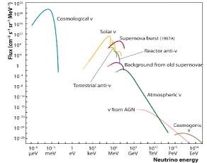
Figure 1.1: Fluxes of neutrinos at different energies. The figure is taken from Ref. [20].

Among these different sources, evidences of neutrino oscillation have come from solar, atmospheric, accelerator and reactor neutrino experiments. Below we discuss about the production mechanism of neutrinos in these type of experiments and describe how different experiments contributed to establish the phenomenon of neutrino oscillation on a firm footing. In this context we will also discuss the production mechanism of the ultra high energy neutrinos. Though the main aim of the ultra high energy neutrino experiments is to study the interaction and production mechanism of the neutrinos from various astrophysical sources, data from these experiments can also be used to constrain the oscillation parameters.

1.4.1 Solar Neutrinos

Solar neutrinos are produced by thermo-nuclear fusion reactions occurring at the core of the Sun. The underlying process is,

$$4p\rightarrow\alpha+2e^{+}+2\nu_{e}.$$

This occurs through proton-proton ($pp$) chain and CNO cycle producing a large number of neutrinos in MeV energy range. Detecting these neutrinos at Earth was important to study the theory of stellar structure and evolution, which is the basis of the standard solar model (SSM). This was the aim of the pioneering experiment by Davis and collaborators using radiochemical Chlorine (${}^{37}{\rm Cl}$) detector [21]. This was sensitive to only electron neutrinos. However, it was found that the observed neutrino flux is only about one third of the solar-model predictions [22, 23]. This deficit constitutes “the solar-neutrino problem”. It was difficult to explain this deficit within the SSM and there were attempts to explain the discrepancy by proposing that the models of the Sun were wrong [24, 25, 26]. Many model independent solutions were proposed [27, 28, 29, 30, 31]. The phenomenon of neutrino oscillations was also considered as one of the possible solutions. In 1981-82, the real time neutrino-electron scattering experiment, Kamiokande [32], became operational which confirmed the deficit observed in the chlorine experiment and also proved that the detected neutrinos actually came from the Sun. Later in 1990 Gallium based experiments, with a lower energy threshold (and thus sensitive to the $pp$ neutrinos) like GALLEX [33] and SAGE [34] (later GNO [35]) corroborated the fact that the measured neutrino signal was indeed smaller than the SSM prediction. The importance of the Ga experiments lies in the detection of the primary $pp$ neutrinos thereby confirming the basic hypothesis of stellar energy generation. Super-Kamiokande (SK), an upgraded version of the Kamiokande experiment [36] further confirmed the solar neutrino deficit with enhanced statistics. But the real breakthrough in solar neutrino physics was due to the advent of the SNO [37, 38] experiment. Because of its sensitivity to both charge current (CC) and neutral current (NC) interactions, it measured simultaneously the contributions from only electron neutrinos and from all three active flavours respectively. By measuring the CC/NC ratio as less than one, SNO established the presence of $\nu_{\mu}$ and $\nu_{\tau}$ flavours in the solar neutrino flux. The NC measurement also confirmed that the measured total neutrino flux was in very good agreement with the SSM predictions. These results clearly showed that neutrinos change their flavour during their way from the production point in the Sun to the detector and the phenomenon of neutrino oscillation emerged as the clear solution to the solar neutrino problem.

1.4.2 Atmospheric Neutrinos

Apart from the solar neutrinos, neutrino oscillation has also been observed in the atmospheric neutrino experiments. Atmospheric neutrinos were first detected in the mines of Kolar Gold Fields of India [39] and at the same time in a gold mine of South Africa [40]. Atmospheric neutrinos result from the interaction of cosmic rays with atomic nuclei in the Earth’s atmosphere, creating pions and kaons, which are unstable and produce neutrinos when they decay in the following manner:

$$\pi^{\pm}(K^{\pm}) \rightarrow \mu^{\pm}+\nu_{\mu}(\bar{\nu}_{\mu}),$$

$$\mu^{\pm} \rightarrow e^{\pm}+\nu_{e}(\bar{\nu}_{e})+\bar{\nu}_{\mu}(\nu_{\mu}).$$

From this decay chain, the expected number of muon neutrinos are about twice that of electron neutrinos. However water Čerenkov detectors like Kamiokande [41], IMB [42, 43] and iron calorimeter detector Sudan2 [44] reported results contrary to this expectation. To reduce the uncertainties in the absolute flux values, these experiments presented results in terms of the double ratio $R$

$$R=\frac{(N_{\mu}/N_{e})_{{\rm obs}}}{(N_{\mu}/N_{e})_{{\rm MC}}},$$ (1.6)

where MC denotes Monte-Carlo simulated ratio. The above experiments found the value of $R$ to be significantly less than one. This became known as the “Atmospheric Neutrino Anomaly”. However two other iron calorimeter detectors Fréjus [45, 46] and Nusex [47] found results consistent with the theoretical expectations. The reduction in $R$ can be explained by either $\nu_{\mu}\rightarrow\nu_{e}$ or $\nu_{\mu}\rightarrow\nu_{\tau}$ oscillations or both. Apart from altering the flavour content of the atmospheric neutrino flux, oscillations can induce the following effect. If the oscillation length is much larger than the height of the atmosphere but smaller than the diameter of the Earth then neutrinos coming from the opposite side of the Earth (upward going neutrinos) will have significant oscillations. This will create a non uniform zenith angle dependence in the observed data. The high statistics SK experiment indeed found this zenith angle dependence in their multi-GeV data establishing neutrino oscillation on a firm footing.

1.4.3 Accelerator Neutrinos

Neutrino oscillations have also been observed from the neutrinos produced in particle accelerators. Neutrino beams produced at a particle accelerator offer the greatest control over the neutrinos being studied. In accelerators, neutrino beam can be produced in two methods: through the decay of pions at rest (DAR) and the decay of pions in flight (DIF). In both the methods, high intensity protons are collided with a fixed target to produce charged pions. In DAR mechanism, the resulting $\pi^{-}$ are being absorbed and $\pi^{+}$ are brought to rest and then they decay in the following manner

$$\pi^{+} \rightarrow \mu^{+}+\nu_{\mu},$$

$$\mu^{+} \rightarrow e^{+}+\nu_{e}+\bar{\nu}_{\mu},$$

to produce $\bar{\nu}_{\mu}$ having maximum allowed energy of 52.8 MeV. The main aim of these type of experiments is to observe clean oscillations in the $\bar{\nu}_{\mu}\rightarrow\bar{\nu}_{e}$ channel as there is no intrinsic $\bar{\nu}_{e}$ background from the source. In the DIF mechanism, the pions decay while traveling in the decay pipe to produce neutrinos and muons. The muons are absorbed and thus one gets pure neutrino or antineutrino beams depending on the polarity of the charged pions. The neutrinos produced in this fashion are essentially beams of $\nu_{\mu}$ and $\bar{\nu}_{\mu}$ with energy ranging from few tens of MeV to GeV. There were several experiments having baselines of the order of few tens of meters looking for neutrino oscillations using neutrinos produced in the accelerators. All of them gave null result except the LSND experiment [49]. LSND reported an excess of events in both $\nu_{\mu}\rightarrow\nu_{e}$ and $\bar{\nu}_{\mu}\rightarrow\bar{\nu}_{e}$ oscillations. It has observed the neutrino events in DIF mode and antineutrino events in DAR mode. The MiniBooNE [50] experiment at Fermilab was proposed to test the LSND results using a different $L$ and $E$ but the same $L/E$ ratio as LSND. It is found that the antineutrino data of MiniBooNE is consistent with the LSND observations. There are also accelerator experiments like K2K [51] and MINOS [52] which have studied the oscillations of the neutrinos in the GeV energy range. These are the long-baseline experiments having baselines around several hundreds of kilometers. K2K has observed neutrino oscillations via muon neutrino disappearance channel ($\nu_{\mu}\rightarrow\nu_{\mu}$) and MINOS has observed events in both appearance ($\nu_{\mu}\rightarrow\nu_{e}$) and disappearance measurements. For these experiments, the neutrino beam power of the accelerators were around few hundreds of KW. The ongoing long-baseline experiment T2K [53] has observed oscillated muon and electron neutrino events at the far detector located 295 km away from the neutrino source. Recently the NO$\nu$A experiment at Fermilab also given its first results which also show a clear evidence of neutrino oscillation [54]. To have enough sensitivity of the sub-dominant electron neutrino appearance channel, T2K/NO$\nu$A as well as the other future generation long-baseline experiments are designed to have beam power of the order of MW. Because of this very high beam power, this type of experiments are often termed as “superbeam” experiments. The high beam power of these experiments also allow to obtain enough statistically significant number of signal events over the expected backgrounds. These accelerator based long-baseline experiments have confirmed the oscillations of the atmospheric neutrinos as the associated $L/E$ in these cases are such that the oscillations are governed by the atmospheric mass square difference $\Delta_{31}$.

1.4.4 Reactor Neutrinos

Another major source of the man-made neutrinos from where oscillations have been observed are the nuclear reactors. In reactors, antineutrinos of the energy around few MeV are produced by the nuclear fission processes. Because of this low energy such experiments are sensitive to only $\bar{\nu}_{e}\rightarrow\bar{\nu}_{e}$ oscillations i.e., they look for a diminution in the $\bar{\nu}_{e}$ flux. Many experiments have searched for oscillation of the reactor neutrinos by detecting the oscillated electron antineutrino events via inverse beta decay (IBD). The measurement of oscillation parameters in the nuclear reactors mainly suffers due to the uncertainties in the strength of the sources, the detector efficiency and the cross sections for neutrino interactions. Thus one needs a good knowledge of the flux. The uncertainties can be minimized by the inclusion of a near detector. The earlier experiments like ILL-Grenoble [55], Rovno [56], Savannah River [57], Gosgen [58], Krasnoyarsk [59], BUGEY [60] searched for oscillations of the reactors antineutrinos at distances $<100$ m from the reactor core. But all these experiments got null results . The next generation longer baseline reactor experiments CHOOZ [62, 63] and Palo Verde [64, 65] looked for oscillations at a distance of 1 km but they also did not report any evidence of neutrino oscillations. The KamLAND [66] experiment, started in 2002, was the first to observe oscillations of the antineutrinos coming out of nuclear reactors. As the baseline of KamLAND was 180 km, it was sensitive to oscillations governed by the mass squared difference $10^{-5}$ eV² which is relevant for the flavour conversion of the solar neutrinos. Thus KamLAND confirmed the oscillations of the solar neutrinos using a man-made neutrino source. Recently the observations of oscillation in the reactor experiments DOUBLE-CHOOZ [67], RENO [68] and Daya Bay [69] have established the non zero value of $\theta_{13}$ with significant confidence level. These experiments have baselines of few kilometers and thus sensitive to oscillations governed by atmospheric mass squared difference of the order of $10^{-3}$ eV².

1.4.5 Ultra High Energy Neutrinos

Ultra high energy (UHE) neutrino telescopes were planned to study the neutrinos from distant astrophysical sources [70]. Currently envisaged astrophysical sources of high energy cosmic neutrinos include for instance, active galactic nuclei (AGN) [71] and gamma ray burst (GRB) fire balls [72]. The production of high energy cosmic neutrinos from sources other than the AGN’s and GRB’s are also possible [73]. In those sources protons are accelerated to very high energies by the Fermi acceleration mechanism [74]. The interactions of these protons with soft photons or matter from the source can give UHE neutrinos. These neutrinos travel a long distance from their source to reach the Earth. The oscillation of this very high energy neutrinos are averaged out due to the long distance and their final flavour composition depends on the initial sources of the neutrinos as different sources can have different initial flavour composition. Recently the IceCube [75] collaboration has reported the results of an all-sky search for UHE neutrino events which was conducted during May 2010 to May 2013. They have detected a total of 37 neutrino events of extraterrestrial origin at $5.7\sigma$ confidence level. These events fall in the energy range between 30 to 2000 TeV. For these observed 37 events, the expected cosmic ray muon background was $8.4\pm 4.2$ and the backgrounds from atmospheric neutrinos were $6.6^{+5.9}_{-1.6}$ events. These results are consistent with the framework of neutrino oscillations over the astronomical distances. The recent IceCube observation of a 2.3 PeV event correspond to the highest-energy neutrino interaction ever observed [76].

1.5 Neutrino Mass Matrix

The observation of non-zero neutrino mass via neutrino oscillations necessitates an extension of the Standard Model. A successful model for neutrino mass needs to explain how neutrinos get their mass as well as why the mass is so tiny. It also requires to explain the observed mixing pattern among the neutrinos. One can simply extend the SM by adding right-handed neutrinos and generate the Dirac neutrino masses in a similar fashion as that of the charged leptons and quarks. But to obtain neutrino mass in the sub eV range, one requires a very small value of the Yukawa coupling i.e., of the order of $10^{-12}$. Introduction of such small coupling constants is generally considered unnatural and one must find a symmetry reason for such smallness. The most elegant way to generate small neutrino mass naturally is the See-Saw mechanism which relates the smallness of neutrino masses to new physics at high scale. In See-Saw mechanism neutrino mass originates from the dimension five operator [77, 78] $\frac{k}{M_{R}}LL\phi\phi$, where $L$ is the lepton doublet, $\phi$ is the Higgs doublet, $k$ is the dimensionful coupling constant and $M_{R}$ is the scale of the beyond Standard Model (BSM) physics. This operator can be realized at the tree level by three ultraviolet completions which are known as Type I [79, 80, 81, 82], Type II [83, 84, 85, 86] and Type III [87] See-Saw. In Type I See-Saw, SM is extended by heavy right-handed singlet neutrinos. In Type II and Type III See-Saw, scalar triplets and fermion triplets are added to the SM respectively. The most economical case among these three is the Type I See-Saw where after the spontaneous symmetry breaking, the neutral component of the Higgs doublet acquires a vacuum expectation value (VEV) $v$ and the light neutrino mass is obtained as

$$m_{\nu}\sim v^{2}/M_{R}.$$ (1.7)

To have neutrino mass around 0.1 eV, one needs $M_{R}$ around $10^{14}$ GeV which is close to the scale of the Grand Unified Theories (GUT). See-Saw mechanism predicts the Majorana nature of the neutrinos which implies that the neutrinos are their own antiparticles. This mechanism also predicts violation of lepton number by two units. In Type I See-Saw the light neutrino mass matrix which is a $3\times 3$ complex matrix in 3 generation, is given by

$$M_{\nu}=M_{D}M_{R}^{-1}M_{D}^{T},$$ (1.8)

where $M_{D}$ is the Dirac mass arising from the Yukawa term $y_{\nu}\bar{L}_{L}\nu_{R}\phi$ and $M_{R}$ is the Majorana mass coming from the Majorana mass term $\bar{\nu}_{R}^{C}\nu_{R}$. In general the neutrino mass matrix $M_{\nu}$ in flavour basis is not diagonal and the complex symmetric $3\times 3$ low energy mass matrix is given by

$$M_{\nu} = V^{*}M_{\nu}^{{\rm diag}}V^{\dagger},$$ (1.9)

$$= \begin{pmatrix}m_{ee}&m_{e\mu}&m_{e\tau}\\ m_{\mu e}&m_{\mu\mu}&m_{\mu\tau}\\ m_{\tau e}&m_{\tau\mu}&m_{\tau\tau}\end{pmatrix},\qquad$$ (1.10)

where, $M_{\nu}^{{\rm diag}}={\rm diag}({m_{1},m_{2},m_{3}})$ and $V=U.P$ denotes the leptonic mixing matrix in a basis where the charged lepton mass matrix is diagonal. $U$ is the PMNS matrix described earlier and $P$ is the diagonal phase matrix of Majorana phases written as

$$P=\text{diag}(1,e^{i\alpha},e^{i{(\beta+\delta)}}).$$ (1.11)

As the elements of this matrix are functions of oscillation parameters (including the Majorana phases), the structure of the low energy mass matrix can be constrained using present experimental data.

1.6 Unknown Oscillation Parameters and Future Prospects: Three Generations

In the last two decades there has been a tremendous progress in the determination of the parameters that describe neutrino oscillation of the three active neutrinos. The solar neutrino experiments and KamLAND have measured the parameters $\theta_{12}$ and $\Delta_{21}$ with considerable precision. The measurements of $\theta_{23}$ and $|\Delta_{31}|$ come from atmospheric neutrino experiments, MINOS and T2K. The reactor experiments have measured the value of $\theta_{13}$ with appreciable precision. We will discuss the present constraints on oscillation parameters from the global analysis of the world neutrino data in the next chapter. At present the unknown oscillation parameters are: (i) the sign of $\Delta_{31}$ or the neutrino mass hierarchy, (ii) the octant of $\theta_{23}$ (i.e., whether $\theta_{23}<45^{\circ}$ or $>45^{\circ}$) and (iii) CP violation in leptonic sector and the precision of $\delta_{CP}$. Apart from these, the following unresolved issues are also of interest: (i) the absolute mass of the neutrinos, (ii) the exact nature of the neutrinos i.e., Dirac or Majorana, (iii) the mechanism of generation of neutrino masses and explanation of their smallness, (iv) non standard interaction (NSI) of the neutrinos, (v) non-unitary neutrino mixing and (vi) CPT violation in neutrino oscillation etc.

The measurement of various oscillation parameters are important not only to understand the exact nature of neutrino oscillation but also for building models in BSM scenario. Many BSM models can be accepted or rejected depending upon their prediction of different oscillation parameters. So a precise measurement of the oscillation parameters can guide towards a successful BSM theory. Determination of $\delta_{CP}$ can also give clue in understanding the present matter-antimatter asymmetry of the universe. The matter-antimatter asymmetry of the universe can be explained by the process of baryogenesis. But the baryogenesis in SM is not sufficient to explain the observed baryon asymmetry of the universe. One option to create additional baryon asymmetry is via leptogenesis in which the decay of heavy right handed neutrinos (for instance those belonging to the See-Saw models) can create lepton asymmetry which can be converted to baryon asymmetry. Different studies show that under certain conditions, it may be possible to connect the leptonic CP phase $\delta_{CP}$ to leptogenesis [88].

There are various current ongoing/future upcoming neutrino oscillation experiments dedicated for determining the remaining unknown oscillation parameters. Below we mention some of the major projects. The beam based long-baseline experiments T2K and NO$\nu$A [89], which are both taking data at present, adopted the off-axis technique which gives a narrow flux at the oscillation maxima to reduce backgrounds at the high energy tail. The experiment T2K itself does not have hierarchy sensitivity and NO$\nu$A has hierarchy sensitivity in a limited range of $\delta_{CP}$ space. But their main aim is to measure the leptonic phase $\delta_{CP}$. The experiments LBNE [91] and LBNO [92] will make use of the on-axis broad band flux to probe oscillation over a wide energy range. Due to the comparatively longer baseline and higher statistics, LBNO and LBNE experiments can measure all the three above mentioned unknowns with significant confidence level. The DAE$\delta$LUS experiment [93] proposes to replace the antineutrinos of the superbeam experiments by the low energy antineutrinos from muon decay at rest and using Gd-doped water Čerenkov detector. This approach will give larger antineutrino event sample as compared to the conventional superbeam technique. The superbeam experiment at the ESS facility [94] proposed to study the physics at the second oscillation maximum for obtaining significant sensitivity towards establishing CP violation.

The atmospheric neutrino experiments ICAL@INO [95] will consist of a magnetized iron calorimeter detector for studying neutrino and antineutrino events separately. These type of detectors are sensitive to muons and they have good energy and direction measurement capability. The Hyper-Kamiokande [96] and PINGU [97] experiments will have large volume water Čerenkov detectors. These detectors can measure energy and direction of both electrons and muons but do not have the charge identification capability. The aim of these experiments are mainly to determine the neutrino mass hierarchy.

In reactor experiments one can have hierarchy sensitivity by using the oscillation interference effect between $\Delta_{31}$ and $\Delta_{32}$. The primary goal of the medium baseline reactor neutrino experiments JUNO [98] and RENO-50 [99] is to determine the mass hierarchy using liquid scintillator detector. These experiments require the precise measurement of the oscillation spectrum with an excellent energy resolution.

Apart from these above mentioned neutrino oscillation experiments, there are also experiments whose primary aim is not to determine the oscillation parameters but still it is possible to probe different oscillation parameters in these experiments. The $0\nu\beta\beta$ and ultra high energy neutrino experiments are example of such experiments. The main aim of the ongoing ultra high energy neutrino detector IceCube at south pole is to understand the origins and acceleration mechanisms of high-energy cosmic rays. But it is also possible to probe different oscillation parameters at IceCube. So a comprehensive phenomenological study regarding the potential of the various neutrino oscillation experiments towards completing the gaps in oscillation physics is extremely relevant at this point.

1.7 Sterile Neutrinos: Beyond Three Generations

Another intriguing aspect of current oscillation picture is the existence of light sterile neutrino. Neutrino oscillation in the standard three flavour picture is now well established from different oscillation experiments. However, the reported observations of $\bar{\nu}_{\mu}$ - $\bar{\nu}_{e}$ oscillations in the LSND experiment [100, 101, 49] and recent confirmation of this by the MiniBooNE experiment [102, 103] with oscillation frequency governed by a mass-squared difference around 1 eV² cannot be accounted for in the above framework. These results motivate the introduction of at least one extra neutrino of mass of the order of eV to account for the three independent mass scales governing solar, atmospheric and LSND oscillations. As we already know that the LEP data on measurement of $Z$-line shape dictates that there can be only three light neutrinos with standard weak interactions, the fourth light neutrino, if it exists must be a Standard Model singlet or sterile. Recently this hypothesis garnered additional support from (i) disappearance of electron antineutrinos in reactor experiments with recalculated fluxes [61] and (ii) deficit of electron neutrinos measured in the solar neutrino detectors GALLEX and SAGE using radioactive sources [104]. The recent ICARUS results [105] however, did not find any evidence for the LSND oscillations. But this does not completely rule out the LSND parameter space and small active-sterile mixing still remains allowed. There are also constraint about existence of an extra relativistic species from the CMB anisotropy measurements [106, 107, 108, 109, 110, 111] which prefer the the effective neutrino number to be greater than three. Recently the combined data of Planck, WMAP polarization and the high multipole results gives $N_{{\rm eff}}=3.36^{+0.68}_{-0.64}$ at 95$\%$ C.L [18]. Clearly this data do not completely rule out the existence of a fourth neutrino species. Thus, the situation with sterile neutrinos remains quite interesting and many future experiments are proposed/planned to test these results and reach a definitive conclusion [112]. In view of these, the study of different phenomenological implications of sterile neutrinos assume an important role. Note that the results in the 3 generation scenario can differ significantly in the presence of sterile neutrino.

1.8 Thesis Overview

In this thesis first we have studied the potential of long-baseline experiments T2K, NO$\nu$A and atmospheric neutrino experiment ICAL@INO to discover CP violation in the leptonic sector. We have also studied the role of the three above mentioned experiments to economise the configuration of future proposed long-baseline experiments LBNO and LBNE in determining the remaining unknowns in neutrino oscillation. We have used the recent IceCube data to put constrain over $\delta_{CP}$ as well as various astrophysical sources. Finally we have studied the structure of the low energy neutrino mass matrix in flavour basis in terms of texture zeros in the presence of one extra light sterile neutrino. The plan of the thesis goes as follows.

In Chapter  2, we give an overview of neutrino oscillation in vacuum and matter elaborating on how matter effect modifies the mass and mixing parameters. We will give derivations of the relevant expressions of the oscillation probabilities. Then we will describe the present status of the oscillation parameters. We will also review the parameter degeneracy in neutrino oscillation and describe how the physics capability of different long-baseline experiments are constrained due to the parameter degeneracy. We will end this chapter by giving a short description about the current/future oscillation experiments which we have studied in this thesis.

In Chapter 3 we will discuss how the various neutrino oscillation parameters can be probed in future oscillation experiments. This chapter will contain the main results of our neutrino oscillation analysis and will be organised as follows: First we will discuss the CP sensitivity of the T2K and NO$\nu$A by taking their projected exposures. Next we discuss how atmospheric neutrino experiment ICAL can improve the CP sensitivity of T2K and NO$\nu$A. We further extend this study taking different exposures and gauge the capability of these setups to discover CP violation and also in measuring the precision of $\delta_{CP}$.

Next we study how the different setups of the LBNO project can be economised by using current/upcoming facilities T2K, NO$\nu$A and ICAL. For our analysis we consider three prospective LBNO setups – CERN-Pyhäsalmi (2290 km), CERN-Slanic (1500 km) and CERN-Fréjus (130 km) and emphasize on the advantage of exploiting the synergies offered by T2K, NO$\nu$A and ICAL in evaluating the adequate exposure which is the minimum exposure required in each case for determining the remaining unknowns of neutrino oscillation i.e hierarchy, octant and $\delta_{CP}$ at a given confidence level.

Then we will carry out a similar analysis as described above, for the LBNE project at Fermilab. Apart from finding the adequate exposure of LBNE in conjunction with T2K, NO$\nu$A and ICAL, we will also quantify the effect of the proposed near detector on systematic errors, examine the role played by the second oscillation cycle in furthering the physics reach of LBNE and present an optimisation study of the neutrino-antineutrino running.

Finally we will study how the recent data of IceCube can constrain the leptonic CP violating phase $\delta_{CP}$. We also use this data to impose constraints on the sources of the neutrinos.

In Chapter 4, we will discuss the structure and properties of neutrino mass matrices and its phenomenological consequences in terms of texture zeros with sterile neutrinos and compare our results with the three generation case. First we will consider the two-zero textures of the low energy neutrino mass matrix in presence of one additional sterile neutrino. We discuss the mass spectrum and the parameter correlations that we find in the various textures. We also present the effective mass governing neutrinoless double beta decay as a function of the lowest mass. Next we will study the phenomenological implications of the one-zero textures of the same neutrino mass matrices in the presence of a sterile neutrino. We study the possible correlations between the sterile mixing angles and the Majorana phases to give a zero element in the mass matrix.

We will summarize and present the impact of our work in the last chapter.

Chapter 2   Neutrino Oscillation

2.1 Overview

In this chapter we discuss the salient features of neutrino oscillation phenomena. As mentioned in the introduction, neutrino oscillation is described by the transition probability from one flavour to another. This is a function of neutrino mass squared differences, mixing angles and the Dirac type CP phase. To understand the dependence of the oscillation probability on different oscillation parameters, one needs to derive the analytic expressions for the same. In the first section of this chapter we will give the derivations of the expressions for the oscillation probability in different scenarios. For the determination of the remaining unknowns in the oscillation sector, one needs to use the information from the past/present experiments as inputs. Thus in the next section, we discuss the current status of the oscillation parameters by comparing global analysis of the world neutrino data as obtained by different groups. Next we discuss what are the difficulties in measuring the unknowns and what are the future facilities that are aimed towards determination of these. This leads us to the discussion about the parameter degeneracies in view of the current oscillation data. We present the hierarchy-$\delta_{CP}$ degeneracy and the octant-$\delta_{CP}$ degeneracy in detail. In the next section we will give the salient features of the present/future oscillation experiments whose physics potential we have studied in this thesis.

2.2 Derivation of Oscillation Probability

In this section we will give the derivations of the expressions for neutrino oscillation probabilities in vacuum and matter and show the dependence of the oscillation probabilities on different oscillation parameters. For neutrinos propagating in vacuum, it is possible to derive exact analytic expressions. For matter one needs to solve the propagation equation using the relevant density profile. For matter of constant density, exact expressions can be derived for the two flavour case. For three flavours, the probability expressions even in constant matter density can be derived only under certain approximations. We will start this section by deriving the vacuum oscillation probability for two flavours which is important to understand the basic mechanism of neutrino oscillation. We also give expressions for generalised $N$ flavour oscillation from which we can easily calculate the three flavour expression. For the matter case, first we will derive the exact two flavour expression in constant density matter and show how the matter effect can modify the vacuum mass and mixing. We will end this section by describing how under the “one mass scale dominance” (OMSD) and the $\alpha-s_{13}$ (double expansion in $\alpha(=\Delta_{21}/\Delta_{31})$ and $\sin\theta_{13}$) approximations one can derive the expressions for probability of the three generation neutrinos in matter of constant density. We will also discuss the validity condition of these approximations.

2.2.1 Two Flavour Oscillation in Vacuum

First let us consider only the first two generations of neutrinos $\nu_{e}$ and $\nu_{\mu}$. In this case the mixing matrix $U$ will be $2\times 2$ unitary matrix parametrised by one mixing angle $\theta$. The relation between the flavour eigenstates and the mass eigenstates can be written as

$$\begin{pmatrix}\nu_{e}\\ \nu_{\mu}\\ \end{pmatrix} = \begin{pmatrix}\cos\theta&\sin\theta\\ -\sin\theta&\cos\theta\\ \end{pmatrix}\begin{pmatrix}\nu_{1}\\ \nu_{2}\\ \end{pmatrix}.$$ (2.1)

The time evolution of the state $\nu_{e}$ after time $t$ is given by

$$|\nu_{e}(t)\rangle=e^{-iE_{1}t}\cos\theta|\nu_{1}\rangle+e^{-iE_{2}t}\sin\theta|\nu_{2}\rangle,$$ (2.2)

where $E_{1}$ and $E_{2}$ are the energies of the mass eigenstates $\nu_{1}$ and $\nu_{2}$ having mass $m_{1}$ and $m_{2}$. The energy $E_{i}$ can be written as (in the units of $c=1$)

$$E_{i}^{2} = p^{2}+m_{i}^{2}$$ (2.3)

$$E_{i} \approx p+\frac{m_{i}^{2}}{2p}.$$ (2.4)

Note that in this plane wave treatment of neutrino oscillation, we have assumed that all the massive neutrinos are of equal momentum $p$. The survival probability of the electron neutrino $\nu_{e}$ is given by

$$P_{ee} = |\langle\nu_{e}|\nu_{e}(t)\rangle|^{2}$$ (2.5)

$$= (\cos^{2}\theta e^{-iE_{1}t}+\sin^{2}\theta e^{-iE_{2}t})(\cos^{2}\theta e^{iE_{1}t}+\sin^{2}\theta e^{iE_{2}t})$$ (2.6)

$$= 1-\sin^{2}2\theta\sin^{2}\{(E_{2}-E_{1})t/2\}.$$ (2.7)

Using Eq. 2.4 in Eq. 2.7 and remembering the fact that in the relativistic limit $p\approx E$ and $t\approx L$ (for $c=1$ and $\hbar=1$) we obtain

$$P_{ee} = 1-\sin^{2}2\theta\sin^{2}\{\Delta_{21}L/4E\}$$ (2.8)

$$= 1-\sin^{2}2\theta\sin^{2}\{1.27\Delta_{21}L/E\},$$ (2.9)

where in Eq. 2.9, $\Delta_{21}=m_{2}^{2}-m_{1}^{2}$ is in eV², $L$ is in km and $E$ is in GeV. The conversion probability i.e., the transition probability from $\nu_{e}\rightarrow\nu_{\mu}$ can be obtained from Eq. 2.9 as

$$P_{e\mu} = 1-P_{ee}$$ (2.10)

$$= \sin^{2}2\theta\sin^{2}\{1.27\Delta_{21}L/E\}.$$ (2.11)

From Eq. 2.11 it is clear that the oscillatory behaviour of the neutrinos is embedded in the term containing $\Delta_{21}$ and this term will go to zero when either the masses $m_{1}$ and $m_{2}$ are equal or when both of them are zero. Thus neutrino oscillation requires non-degenerate and non-zero masses of neutrinos. Another important feature of Eq. 2.11 is that, this expression is not sensitive to the octant of $\theta$ (i.e., $\theta<45^{\circ}$ or $>45^{\circ}$) and the sign of $\Delta_{21}$ as the transformation defined by $\theta\rightarrow\pi/2-\theta$ and $\Delta_{21}\rightarrow-\Delta_{21}$, leaves this equation unaltered.

Here it is important to note that neutrino oscillation is also characterised by the value of $L$ and $E$ under consideration. For a combination of $L$ and $E$ such that the oscillatory term $\Delta_{21}L/4E$ goes to zero, there will be no oscillation. On the other hand if we consider a very high value of $L$, then there will be very large number of oscillation cycles at smaller values of $E$. Hence the oscillation will be averaged out and probabilities will not depend explicitly on the masses of the neutrinos any more. This is the case for ultra high energy neutrinos which travel a large distance in vacuum to reach the Earth. The maximum oscillation of the neutrinos can be obtained under the condition

$$1.27\Delta_{21}L/E=n\pi/2,$$ (2.12)

where $n=1$ correspond to first oscillation maxima. This is the case for accelerator based long-baseline neutrino experiments. Here the accelerators are designed such that the neutrino flux peaks at the energies where the oscillation is maximum. For example in the T2K experiment, the distance from source to detector is 295 km and the neutrino flux peaks at 0.6 GeV. Putting this number in the above equation, for $n=1$ we get the value of the mass squared difference as $2.5\times 10^{-3}$ eV² which is close to the current best-fit of the atmospheric mass squared difference.

Before generalising the above formula for $N$ flavours, we would like to give another alternative method to derive the same oscillation formula. This formalism will be important at the time of deriving the oscillation formula in matter. The time dependent Schrödinger equation in the mass basis can be written as

$$i\frac{\partial\nu_{i}}{\partial t} = H_{M}\nu_{i},$$ (2.13)

where $H_{M}$ is the effective Hamiltonian in the mass basis and $\nu_{i}$ is the mass eigenstate. For the case of two generations of neutrinos this can be written as

$$H_{M}=\begin{pmatrix}E_{1}&0\\ 0&E_{2}\\ \end{pmatrix}.$$ (2.14)

Using Eq. 2.4 one gets

$$H_{M}=EI+\frac{1}{2E}\begin{pmatrix}m_{1}^{2}&0\\ 0&m_{2}^{2}\\ \end{pmatrix},$$ (2.15)

where $I$ is the $2\times 2$ identity matrix. Here we would like to mention that as the common diagonal terms affect both the neutrino flavours in the same way, they do not contribute in the final expressions of probability. Thus we can always add or subtract any diagonal term from the effective Hamiltonian $H$. Using Eq. 2.1, we convert the Eq. 2.13 into flavour basis and obtain the following equation for the two flavour scenario

$$i\frac{\partial}{\partial t}\begin{pmatrix}\nu_{e}\\ \nu_{\mu}\\ \end{pmatrix} = H_{F}\begin{pmatrix}\nu_{e}\\ \nu_{\mu}\\ \end{pmatrix},$$ (2.16)

where $H_{F}$ is the effective Hamiltonian in the flavour basis and is given by

$$H_{F} = U^{\dagger}\begin{pmatrix}m_{1}^{2}/2E&0\\ 0&m_{2}^{2}/2E\\ \end{pmatrix}U.$$ (2.17)

Subtracting $\frac{m_{1}^{2}+m_{2}^{2}}{4E}$ from the diagonal elements, the above equation can be simplified to

$$H_{F} = \frac{1}{4E}\begin{pmatrix}-\Delta_{21}\cos 2\theta&\Delta_{21}\sin 2\theta\\ \Delta_{21}\sin 2\theta&\Delta_{21}\cos 2\theta\end{pmatrix},$$ (2.18)

and Eq. 2.16 can be explicitly written as

$$i\frac{\partial\nu_{e}}{\partial t} = -a\nu_{e}+b\nu_{\mu},$$ (2.19)

$$i\frac{\partial\nu_{\mu}}{\partial t} = b\nu_{e}+a\nu_{\mu},$$ (2.20)

where

$$a=\frac{\Delta_{21}\cos 2\theta}{4E},\hskip 8.53581ptb=\frac{\Delta_{21}\sin 2\theta}{4E}.$$ (2.21)

Solving the two coupled differential Eqs. 2.19 and 2.20 we obtain

$$\nu_{e}(t) = A_{1}e^{-i\omega t}+A_{2}e^{i\omega t},$$ (2.22)

$$\nu_{\mu}(t) = B_{1}e^{-i\omega t}+B_{2}e^{i\omega t},$$ (2.23)

with the condition $|\nu_{e}(t)|^{2}+|\nu_{\mu}(t)|^{2}=1$, where $\omega^{2}=a^{2}+b^{2}=\left(\frac{\Delta_{21}}{4E}\right)^{2}$. Using initial conditions $\nu_{e}(0)=1$ and $\nu_{\mu}(0)=0$, we obtain

$$A_{1}=\sin^{2}\theta,~{}A_{2}=\cos^{2}\theta,~{}B_{1}=\sin\theta\cos\theta,~{}B_{2}=-\sin\theta\cos\theta.$$ (2.24)

This gives the transition probability $\nu_{e}\rightarrow\nu_{\mu}$ as

$$P_{e\mu}=|\nu_{\mu}(t)|^{2}=\sin^{2}2\theta\sin^{2}\{1.27\Delta_{21}L/E\}.$$ (2.25)

2.2.2 $N$ Flavour Oscillation in Vacuum

In this section we derive the vacuum oscillation probability for a generalised $N$ flavour oscillation scenario. For $N$ flavours, the mixing matrix $U$ is a $N\times N$ unitary matrix parametrised by $N(N-1)/2$ number of mixing angles and $(N-1)(N-2)/2$ number of phases. At time $t=0$, the flavour eigenstates are written as

$$|\nu_{\alpha}(0)\rangle=\sum_{i=1}^{N}U_{\alpha i}|\nu_{i}\rangle.$$ (2.26)

Here the index $\alpha$ corresponds to all the $N$ flavours of neutrinos. After time $t$, the flavour states will evolve to

$$|\nu_{\alpha}(t)\rangle=\sum_{i}^{N}U_{\alpha i}e^{-iE_{i}t}|\nu_{i}\rangle.$$ (2.27)

The oscillation probability $\nu_{\alpha}\rightarrow\nu_{\beta}$ ($P_{\alpha\beta}$) is given by

$$P_{\alpha\beta} = \left|\langle\nu_{\beta}|\nu_{\alpha}(t)\rangle\right|^{2}$$ (2.28)

$$= \left|\sum_{i=1}^{N}U_{\alpha i}U_{\beta i}^{*}e^{-iE_{i}t}\right|^{2}$$ (2.29)

$$= \sum_{i=1}^{N}\sum_{j=1}^{N}(U_{\alpha i}U_{\beta i}^{*}e^{-iE_{i}t})(U_{\alpha j}^{*}U_{\beta j}e^{iE_{j}t})$$ (2.30)

$$= \sum_{i=j}|U_{\alpha i}|^{2}|U_{\beta i}|^{2}+\sum_{i\neq j}U_{\alpha i}U_{\beta j}U_{\alpha j}^{*}U_{\beta i}^{*}e^{-i(E_{i}-E_{j})t}.$$ (2.31)

Using the relation

$$\left|\sum_{i}U_{\alpha i}U_{\beta i}^{*}\right|^{2}=\sum_{i}|U_{\alpha i}|^{2}|U_{\beta i}|^{2}+\sum_{i\neq j}U_{\alpha i}U_{\beta j}U_{\alpha j}^{*}U_{\beta i}^{*},$$ (2.32)

in Eq. 2.31 we obtain

$$P_{\alpha\beta}= \left|\sum_{i}U_{\alpha i}U_{\beta i}^{*}\right|^{2}-\sum_{i\neq j}U_{\alpha i}U_{\beta j}U_{\alpha j}^{*}U_{\beta i}^{*}$$ (2.33)

$$+\sum_{i\neq j}U_{\alpha i}U_{\beta j}U_{\alpha j}^{*}U_{\beta i}^{*}e^{-i(E_{i}-E_{j})t}.$$

Using the unitarity relation

$$\sum_{i}U_{\alpha i}U_{\beta i}^{*}=\delta_{\alpha\beta},$$ (2.34)

we obtain

$$P_{\alpha\beta}=~{} \delta_{\alpha\beta}-\bigg{[}\sum_{i<j}U_{\alpha i}U_{\beta j}U_{\alpha j}^{*}U_{\beta i}^{*}+\sum_{i<j}U_{\alpha i}^{*}U_{\beta j}^{*}U_{\alpha j}U_{\beta i}\bigg{]}$$ (2.35)

$$+\bigg{[}\sum_{i<j}U_{\alpha i}U_{\beta j}U_{\alpha j}^{*}U_{\beta i}^{*}e^{-i(E_{i}-E_{j})t}+\sum_{i<j}U_{\alpha i}^{*}U_{\beta j}^{*}U_{\alpha j}U_{\beta i}e^{i(E_{i}-E_{j})t}\bigg{]}$$

$$=~{} \delta_{\alpha\beta}-2\sum_{i<j}\text{Re}\big{(}U_{\alpha i}U_{\beta j}U_{\alpha j}^{*}U_{\beta i}^{*}\big{)}$$ (2.36)

$$+2\sum_{i<j}\text{Re}\big{(}U_{\alpha i}U_{\beta j}U_{\alpha j}^{*}U_{\beta i}^{*}\big{)}\cos(E_{i}-E_{j})t$$

$$+2\sum_{i<j}\text{Im}\big{(}U_{\alpha i}U_{\beta j}U_{\alpha j}^{*}U_{\beta i}^{*}\big{)}\sin(E_{i}-E_{j})t.$$

In deriving Eq. 2.36 we used the following fact that if $z$ is a complex number then

$$z+z^{*} = 2~{}\text{Re}(z),$$ (2.37)

$$z-z^{*} = 2~{}i~{}\text{Im}(z).$$ (2.38)

Thus the final form of the oscillation probability for $N$ generations is

$$P_{\alpha\beta}=~{} \delta_{\alpha\beta}-4\sum_{i<j}\text{Re}\big{(}U_{\alpha i}U_{\beta j}U_{\alpha j}^{*}U_{\beta i}^{*}\big{)}\sin^{2}\{\Delta_{ij}L/4E\}$$ (2.39)

$$+2\sum_{i<j}\text{Im}\big{(}U_{\alpha i}U_{\beta j}U_{\alpha j}^{*}U_{\beta i}^{*}\big{)}\sin\{2\Delta_{ij}L/4E\},$$

where $\Delta_{ij}=m_{i}^{2}-m_{j}^{2}$. Using the Eq. 2.39, it is now straightforward to derive the corresponding expressions for three flavours.

2.2.3 Two Flavour Oscillation in Matter

Neutrino propagation in matter modifies the neutrino oscillation probabilities. When active neutrino flavours traverse through matter, their evolution equation is affected by the potentials due to the interactions with the medium through coherent forward elastic weak charge current (CC) and neutral current (NC) scatterings. The charge current interactions affect only $\nu_{e}$ since normal matter consists of electron, proton and neutron but the neutral current interactions affect all the three active neutrinos. These interactions can be represented by the Feynman diagrams given in Fig. 2.1.

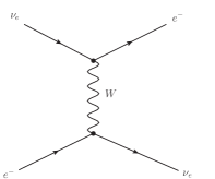
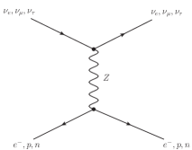
Figure 2.1: CC and NC interactions of neutrinos.

As the NC scattering potential modifies the propagation equation for all the neutrinos in the same way, it does not have any effect on the final expressions of neutrino oscillation probabilities. The CC interaction affects only the electron neutrinos and it modifies the probability expression significantly. The effective Hamiltonian for the CC interaction can be written as

$$H_{{\rm eff}}=\frac{G_{F}}{\sqrt{2}}\big{[}\bar{e}\gamma_{\mu}(1-\gamma_{5})\nu_{e}\big{]}\big{[}\bar{\nu}_{e}\gamma^{\mu}(1-\gamma_{5})e\big{]},$$ (2.40)

where $G_{F}$ is the Fermi constant. Using the Fierz transformation we obtain

$$H_{{\rm eff}}=\frac{G_{F}}{\sqrt{2}}\big{[}\bar{e}\gamma_{\mu}(1-\gamma_{5})e\big{]}\big{[}\bar{\nu}_{e}\gamma^{\mu}(1-\gamma_{5})\nu_{e}\big{]}.$$ (2.41)

The interaction potential is given by the average of the effective Hamiltonian over the electron background i.e.,

$$\bar{H}_{{\rm eff}}=\frac{G_{F}}{\sqrt{2}}\langle\bar{e}\gamma_{\mu}(1-\gamma_{5})e\rangle\big{[}\bar{\nu}_{e}\gamma^{\mu}(1-\gamma_{5})\nu_{e}\big{]}.$$ (2.42)

In the non-relativistic limit using the explicit forms of Dirac spinors one can show that [117, 118]

$$\langle\bar{e}\gamma_{\mu}\gamma_{5}e\rangle \sim \text{spin},$$ (2.43)

$$\langle\bar{e}\gamma_{i}e\rangle \sim \text{velocity},$$ (2.44)

$$\langle\bar{e}\gamma_{0}e\rangle = N_{e},$$ (2.45)

where $N_{e}$ is the electron number density of the medium. In the rest frame of unpolarised electrons only $N_{e}$ term is non-zero and thus we obtain

$$\bar{H}_{{\rm eff}} = \sqrt{2}G_{F}N_{e}\bar{\nu}_{eL}\gamma^{0}\nu_{eL}$$ (2.46)

$$= v_{CC}\bar{\nu}_{eL}\gamma^{0}\nu_{eL}$$ (2.47)

$$= v_{CC}j_{\nu},$$ (2.48)

where $\nu_{eL}=\frac{1-\gamma_{5}}{2}\nu_{e}$, $j_{\nu}=\bar{\nu}_{eL}\gamma^{0}\nu_{eL}$ and $v_{CC}$ is the interaction potential given by

$$v_{CC}=\sqrt{2}G_{F}N_{e}.$$ (2.49)

For antineutrinos, we have to consider the charge conjugate field $\nu_{eL}^{C}$ i.e.,

$$j_{\nu}^{C} = \bar{\nu}_{eL}^{C}\gamma^{0}\nu_{eL}^{C}$$ (2.50)

$$= -\nu_{eL}^{T}C^{-1}\gamma^{0}C\bar{\nu}_{eL}^{T},$$ (2.51)

where $C$ is the charge conjugation operator and we have used the fact that

$$\nu_{eL}^{C} = C\bar{\nu}_{eL}^{T},$$ (2.52)

$$\bar{\nu}_{eL}^{C} = -\nu_{eL}^{T}C^{-1}.$$ (2.53)

Using the property

$$C^{-1}\gamma^{0}C=(-\gamma^{0})^{T},$$ (2.54)

we obtain

$$j_{\nu}^{C} = \nu_{eL}^{T}(\gamma^{0})^{T}\bar{\nu}_{eL}^{T}$$ (2.55)

$$= -\bar{\nu}_{eL}\gamma^{0}\nu_{eL},$$ (2.56)

and thus for antineutrinos the effective Hamiltonian becomes

$$\bar{H}_{{\rm eff}} = -\sqrt{2}G_{F}N_{e}\bar{\nu}_{eL}\gamma^{0}\nu_{eL},$$ (2.57)

which gives

$$\bar{v}_{CC}=-\sqrt{2}G_{F}N_{e},$$ (2.58)

for antineutrinos.

With the inclusion of the potential $v_{CC}$, the evolution Eq. 2.16 becomes

$$i\frac{\partial}{\partial t}\begin{pmatrix}\nu_{e}\\ \nu_{\mu}\\ \end{pmatrix}=H_{F}^{{\rm matt}}\begin{pmatrix}\nu_{e}\\ \nu_{\mu}\\ \end{pmatrix},$$ (2.59)

with

$$H_{F}^{{\rm matt}}=\begin{pmatrix}-\frac{\Delta_{21}}{4E}\cos 2\theta+v_{CC}&\frac{\Delta_{21}}{4E}\sin 2\theta\\ \frac{\Delta_{21}}{4E}\sin 2\theta&\frac{\Delta_{21}}{4E}\cos 2\theta\\ \end{pmatrix}.$$ (2.60)

By defining

$$A=2\sqrt{2}G_{F}N_{e}E,$$ (2.61)

and subtracting $\frac{A}{4E}$ from the diagonal elements, Eq. 2.60 simplifies to

$$H_{F}^{{\rm matt}}=\frac{1}{4E}\begin{pmatrix}A-\Delta_{21}\cos 2\theta&\Delta_{21}\sin 2\theta\\ \Delta_{21}\sin 2\theta&-A+\Delta_{21}\cos 2\theta\\ \end{pmatrix}.$$ (2.62)

The energy eigenvalues of $H_{F}^{{\rm matt}}$ are obtained by diagonalising the above:

$$E_{1,2}=\frac{1}{4E}\left[A\pm\sqrt{(-A+\Delta_{21}\cos 2\theta)^{2}+(\Delta_{21}\sin 2\theta)^{2}}\right].$$ (2.63)

Now remembering the fact that $E_{2}-E_{1}=(m_{2}^{2}-m_{1}^{2})/2E$, we obtain the modified mass squared difference in the presence of matter as

$$\Delta_{21}^{M}=\sqrt{(-A+\Delta_{21}\cos 2\theta)^{2}+(\Delta_{21}\sin 2\theta)^{2}}.$$ (2.64)

The above equation shows how the masses are modified in the presence of the matter term $A$. Now we will see how the mixing is being modified. Let us assume that the modified mixing angle in the presence of matter is $\theta_{M}$ and we call the modified mixing matrix as $U_{M}$. The matrix $H_{F}^{{\rm matt}}$ which is now in flavour basis can be converted into mass basis by the transformation $H_{M}^{{\rm matt}}=U_{M}^{\dagger}H_{F}^{{\rm matt}}U_{M}$. Setting the off-diagonal terms as zero we obtain

$$\tan 2\theta_{M}=\frac{\Delta_{21}\sin 2\theta}{-A+\Delta_{21}\cos 2\theta},$$ (2.65)

and the expression for the probability for $P_{e\mu}$ becomes

$$P_{e\mu}=\sin^{2}2\theta_{M}\sin^{2}(1.27\Delta_{21}^{M}L/E).$$ (2.66)

Note that, the expression for the vacuum oscillation probability was not sensitive to the sign of $\Delta_{21}$ and octant of $\theta$ but due the modification in mass and mixing, the expression is sensitive to both of them. Another interesting phenomenon in this case is the MSW (Mikheyev-Smirnov-Wolfenstein) resonance. This happens when

$$\Delta_{21}\cos 2\theta = A$$ (2.67)

$$= 0.76\times 10^{-4}\bigg{[}\frac{\rho}{{\rm gm/cc}}\bigg{]}\bigg{[}\frac{E}{{\rm GeV}}\bigg{]}{\rm eV}^{2}.$$ (2.68)

If this condition is satisfied then we see that the mixing angle becomes maximal i.e., $\pi/4$. This leads to the possibility of total transitions between the two flavours. Since for neutrinos $A$ is positive, resonance can only occur for $\Delta_{21}>0$ and $\theta<\pi/4$ or $\Delta_{21}<0$ and $\theta>\pi/4$. For antineutrinos the resonance condition is given by $\Delta_{21}>0$ and $\theta>\pi/4$ or $\Delta_{21}<0$ and $\theta<\pi/4$. From this it is clear that the enhancement of the neutrino and antineutrino probabilities depend on the sign of $\Delta_{21}$ and octant of $\theta$. Thus the experimental observation of this resonance effect can lead to the determination of the same.

2.2.4 Three Flavour Oscillation in Matter: The OMSD Approximation

In this section we discuss how the probability expressions can be derived, for three generations in matter of constant density. As we have mentioned earlier, in this case it is difficult to find exact analytic expressions for the probabilities. In this section we will use the one mass scale dominance (OMSD) approximation [119] in deriving the same. For the three generation scenario the effective Hamiltonian in the flavour basis takes the following form

$$H_{F}^{{\rm matt}}=U\begin{pmatrix}0&0&0\\ 0&\Delta_{21}/2E&0\\ 0&0&\Delta_{31}/2E\\ \end{pmatrix}U^{\dagger}+\begin{pmatrix}\sqrt{2}G_{F}N_{e}&0&0\\ 0&0&0\\ 0&0&0\\ \end{pmatrix}.$$ (2.69)

The OMSD approximation implies that the measured small mass squared difference $\Delta_{21}$ can be neglected as compared to $\Delta_{31}$. Under this approximation, the effects of the solar mixing angle $\theta_{12}$ and of the CP violating phase in $U$ become inconsequential and $U$ simply becomes

$$U=R_{23}R_{13}=\begin{pmatrix}1&0&0\\ 0&c_{23}&s_{23}\\ 0&-s_{23}&c_{23}\\ \end{pmatrix}\begin{pmatrix}c_{13}&0&s_{13}\\ 0&1&0\\ -s_{13}&0&c_{13}\\ \end{pmatrix}.$$ (2.70)

Using this, the energy eigenvalues of $H_{F}^{{\rm matt}}$ can be obtained as

$$E_{1,3} = \frac{1}{4E}\left[\Delta_{31}+A\pm\sqrt{(\Delta_{31}\cos 2\theta_{13}-A)^{2}+(\Delta_{31}\sin 2\theta_{13})^{2}}\right],$$ (2.71)

$$E_{2} = 0.$$ (2.72)

In this approximation the modified mixing matrix $U_{M}$ can be written as

$$U_{M}=R_{23}R_{13}^{M}.$$ (2.73)

Thus matter effect do not modify the mixing angle $\theta_{23}$. This can be qualitatively understood from the fact that matter effect only modifies the evolution equation for $\nu_{e}$ and mixing of $\nu_{e}$ with the mass eigenstates states does not involve the mixing angle $\theta_{23}$. Again in a similar manner as described in the two flavour case, the relation between the modified mixing angle $\theta_{13}^{M}$ and the vacuum angle $\theta_{13}$ can be derived as

$$\tan 2\theta_{13}^{M}=\frac{\Delta_{31}\sin 2\theta_{13}}{\Delta_{31}\cos 2\theta_{13}-A}.$$ (2.74)

In this case the expression for transition probability $P_{\alpha\beta}$ can be derived from Eq. 2.39 by replacing $U$ by $U_{M}$. Below we write the probability formula derived under the OMSD approximation for the transition $\nu_{e}\rightarrow\nu_{\mu}$:

$$P_{e\mu} = \sin^{2}\theta_{23}\sin^{2}2\theta_{13}^{M}\sin^{2}(\Delta_{31}^{M}L/4E),$$ (2.75)

$$P_{\mu\mu} = 1-\cos^{2}\theta_{13}^{M}\sin^{2}2\theta_{23}\sin^{2}\left(\frac{\Delta_{31}+A+\Delta_{31}^{M}}{4E}\right)L$$

$$~{}-\sin^{2}\theta_{13}^{M}\sin^{2}\theta_{23}\sin^{2}\left(\frac{\Delta_{31}+A-\Delta_{31}^{M}}{4E}\right)L$$

$$~{}-\sin^{4}\theta_{23}\sin^{2}2\theta_{13}^{M}\sin^{2}\left(\frac{\Delta_{31}^{M}L}{4E}\right),$$

with

$$\Delta_{31}^{M}=\sqrt{(\Delta_{31}\cos 2\theta_{13}-A)^{2}+(\Delta_{31}\sin 2\theta_{13})^{2}}.$$ (2.77)

We will give the expression for the $P_{ee}$ channel in the appendix.

Let us now briefly discuss the validity condition of the OMSD approximation. The condition on the neutrino energy and baseline for the OMSD approximation to be valid is

$$\frac{\Delta_{21}L}{E}\ll 1.$$ (2.78)

This corresponds to $L/E\ll 10^{4}$ km/GeV which is mainly the case for the atmospheric neutrinos. OMSD approximation also needs large values of $\theta_{13}$ because the terms appearing with $\Delta_{21}$ can only be dropped if they are small compared to the leading order term containing $\theta_{13}$. We will discuss this point again after discussing the $\alpha-s_{13}$ approximation which we will use in the next subsection to derive the most general three flavour oscillation expression in matter.

2.2.5 Three Flavour Oscillation in Matter: The $\alpha-s_{13}$ Approximation

In this subsection we will give the derivation of the approximate three flavour probability expressions using the series expansion method [120] in a constant matter density. We will study expansions in terms of the mass hierarchy parameter $\alpha=\Delta_{21}/\Delta_{31}$ and mixing parameter $s_{13}=\sin\theta_{13}$ keeping terms up to second order. The effective Hamiltonian in flavour basis can be written as

$$H_{F}^{{\rm matt}}=\frac{\Delta_{31}}{2E}\big{[}U\text{diag}(0,\alpha,1)U^{\dagger}+\text{diag}(\hat{A},0,0)\big{]},$$ (2.79)

where $\hat{A}=A/\Delta_{31}$. In order to derive the double expansion, we write the above Hamiltonian as

$$H_{F}^{{\rm matt}}=\frac{\Delta_{31}}{2E}R_{23}U_{\delta}MU_{\delta}^{\dagger}R_{23}^{T},$$ (2.80)

where $U_{\delta}=\text{diag}(1,1,e^{i\delta_{CP}})$. We define,

$$H_{F}^{\prime{{\rm matt}}} = \frac{\Delta_{31}}{2E}M$$ (2.81)

$$= \frac{\Delta_{31}}{2E}\left[R_{13}R_{12}\text{diag}(0,\alpha,1)R_{12}^{T}R_{13}^{T}+\text{diag}(\hat{A},0,0)\right]$$ (2.82)

$$= \begin{pmatrix}s_{12}^{2}c_{13}^{2}\alpha+s_{13}^{2}+\hat{A}&\alpha c_{12}c_{13}s_{12}&s_{13}c_{13}(1-\alpha s_{12}^{2})\\ s_{12}c_{12}c_{13}\alpha&\alpha c_{12}^{2}&-\alpha c_{12}s_{12}s_{13}\\ s_{13}c_{13}(1-\alpha s_{12}^{2})&-s_{12}c_{12}s_{13}\alpha&\alpha s_{12}^{2}s_{13}^{2}+c_{13}^{2}\\ \end{pmatrix}.$$ (2.83)

Diagonalisation is performed using perturbation theory up to second order in the small parameters $\alpha$ and $s_{13}$ i.e.,

$$M=M^{0}+M^{1}+M^{2},$$ (2.84)

where

$$M^{0}=\text{diag}(\hat{A},0,1)=\text{diag}(\lambda_{1}^{0},\lambda_{2}^{0},\lambda_{3}^{0}),$$ (2.85)

$$M^{1}=\begin{pmatrix}\alpha s_{12}^{2}&\alpha s_{12}c_{12}&s_{13}\\ \alpha s_{12}c_{12}&\alpha c_{12}^{2}&0\\ s_{13}&0&0\\ \end{pmatrix},$$ (2.86)

$$M^{2}=\begin{pmatrix}s_{13}^{2}&0&-\alpha s_{13}s_{12}^{2}\\ 0&0&-\alpha s_{13}s_{12}c_{12}\\ -\alpha s_{13}s_{12}^{2}&-\alpha s_{13}s_{12}c_{12}&-s_{13}^{2}\\ \end{pmatrix}.$$ (2.87)

For eigenvalues we write

$$\lambda_{i}=\lambda_{i}^{0}+\lambda_{i}^{1}+\lambda_{i}^{2},$$ (2.88)

and for the eigenvectors we write

$$v_{i}=v_{i}^{0}+v_{i}^{1}+v_{i}^{2}.$$ (2.89)

Since $M^{0}$ is already diagonal we have

$$v_{i}^{0}=e_{i},$$ (2.90)

i.e.,

$$v_{1}^{0}=\begin{pmatrix}1\\ 0\\ 0\\ \end{pmatrix},\hskip 8.53581ptv_{2}^{0}=\begin{pmatrix}0\\ 1\\ 0\\ \end{pmatrix},\hskip 8.53581ptv_{3}^{0}=\begin{pmatrix}0\\ 0\\ 1\\ \end{pmatrix}.$$ (2.91)

Now the first and second order corrections to the eigenvalues are given by

$$\lambda_{i}^{1} = M_{ii}^{1}=\langle v_{i}^{0}|M^{1}|v_{i}^{0}\rangle,$$ (2.92)

$$\lambda_{i}^{2} = M_{ii}^{2}+\sum_{j\neq i}\frac{(M_{ii}^{1})^{2}}{\lambda_{i}^{0}-\lambda_{j}^{0}},$$ (2.93)

and the corrections to the eigenvectors are given by

$$v_{i}^{1} = \sum_{j\neq i}\frac{M_{ij}^{1}}{\lambda_{i}^{0}-\lambda_{j}^{0}}e_{j},$$ (2.94)

$$v_{i}^{2} = \sum_{j\neq i}\frac{1}{\lambda_{i}^{0}-\lambda_{j}^{0}}\big{[}M_{ij}^{2}+(M^{1}v_{i}^{1})_{j}-\lambda_{i}^{1}(v_{i}^{1})_{j}\big{]}e_{j}.$$ (2.95)

Using Eqs. 2.92 and 2.93 and keeping in mind the fact that $E_{i}=\frac{\Delta_{31}}{2E}\lambda_{i}$, we obtain the following expressions for energy eigenvalues

$$E_{1} = \frac{\Delta_{31}}{2E}\big{(}\hat{A}+\alpha s_{12}^{2}+s_{13}^{2}\frac{\hat{A}}{\hat{A}-1}+\alpha^{2}\frac{\sin^{2}2\theta_{12}}{4\hat{A}}\big{)},$$ (2.96)

$$E_{2} = \frac{\Delta_{31}}{2E}\big{(}\alpha c_{12}^{2}-\alpha^{2}\frac{\sin^{2}2\theta_{12}}{4\hat{A}}\big{)},$$ (2.97)

$$E_{3} = \frac{\Delta_{31}}{2E}\big{(}1-s_{13}^{2}\frac{\hat{A}}{\hat{A}-1}\big{)},$$ (2.98)

and using Eqs. 2.94 and 2.95 we get the three eigenvectors as

$$v_{1} = \begin{pmatrix}1\\ \frac{\alpha\sin 2\theta_{12}}{2\hat{A}}+\frac{\alpha^{2}\sin 4\theta_{12}}{4\hat{A}^{2}}\\ \frac{s_{13}}{\hat{A}-1}-\frac{\hat{A}\alpha s_{13}s_{12}^{2}}{(\hat{A}-1)^{2}}\\ \end{pmatrix},\hskip 8.53581ptv_{2}=\begin{pmatrix}-\frac{\alpha\sin 2\theta_{12}}{2\hat{A}}-\frac{\alpha^{2}\sin 4\theta_{12}}{4\hat{A}^{2}}\\ 1\\ \frac{\alpha s_{13}\sin 2\theta_{12}(\hat{A}+1)}{2\hat{A}}\\ \end{pmatrix},$$ (2.99)

$$\text{and}\hskip 8.53581ptv_{3} = \begin{pmatrix}-\frac{s_{13}}{\hat{A}-1}+\frac{\hat{A}\alpha s_{13}s_{12}^{2}}{(\hat{A}-1)^{2}}\\ \frac{\hat{A}\alpha s_{13}\sin 2\theta_{12}}{2(\hat{A}-1)}\\ 1\\ \end{pmatrix}.$$

With these, the modified mixing matrix in matter is given by

$$U_{M}=R_{23}U_{\delta}W,$$ (2.100)

with $W=(v_{1},v_{2},v_{3})$.

Now it is straightforward to obtain the expressions for oscillation probabilities from Eq. 2.39 using the elements of $U_{M}$ and expressions derived in the Eqs. 2.96, 2.97 and 2.98. Below we write down the expressions corresponding to the transition probability $\nu_{\mu}\rightarrow\nu_{e}$ and the leading order term for $\nu_{\mu}\rightarrow\nu_{\mu}$:

$$P_{\mu e}=~{} 4s_{13}^{2}s_{23}^{2}\frac{\sin^{2}(\hat{A}-1)\Delta}{(\hat{A}-1)^{2}}$$ (2.101)

$$+2\alpha s_{13}\sin 2\theta_{12}\sin 2\theta_{23}\cos(\Delta+\delta_{CP})\frac{\sin\hat{A}\Delta}{\hat{A}}\frac{\sin(\hat{A}-1)\Delta}{\hat{A}-1}$$

$$+\alpha^{2}\sin^{2}2\theta_{12}c_{23}^{2}\frac{\sin^{2}\hat{A}\Delta}{\hat{A}^{2}},$$

$$P_{\mu\mu}=~{} 1-\sin^{2}2\theta_{23}\sin^{2}\Delta+\text{higher order terms},$$ (2.102)

where $\Delta=\Delta_{31}/4E$. For antineutrinos, the relevant formula can be obtained by $\hat{A}\rightarrow-\hat{A}$ and $\delta_{CP}\rightarrow-\delta_{CP}$. The expressions for IH can be obtained by replacing $\Delta$ by $-\Delta$ and $\hat{A}$ by $-\hat{A}$. We will give the full expressions for $P_{\mu\mu}$ and $P_{ee}$ in the appendix.

Formally this calculation is based upon the approximation $\alpha,s_{13}\ll 1$ and no explicit assumptions about the values of $L/E$ are made. However, we remark that the series expansion formula is no longer valid as soon as $\alpha\Delta=\Delta_{21}L/4E$ becomes order of unity, i.e., when the oscillatory behaviour is governed by the mass squared difference $\Delta_{21}$. As this is not the case for the current generation long-baseline experiments, we will use this formula to understand the oscillation physics for the same. But this condition can occur for very long baselines and/or very low energies where these equations will no longer be applicable.

After discussing the validity of the $\alpha-s_{13}$ approximation, let us go back to the validity of the OMSD approximation. We have already discussed the fact that the OMSD approximation will fail if $\theta_{13}$ is too small. If we compare the first and second terms of Eq. 2.101, it is obvious that the first term can be safely neglected in comparison to second if

$$\sin\theta_{13}\gg\alpha.$$ (2.103)

Now using current best-fit values of $\Delta_{21}$ and $\Delta_{31}$, the above condition translates to

$$\sin\theta_{13}\gg 0.03,$$ (2.104)

which is consistent with the current value of this parameter.

Note that, as the OMSD approximation is exact in $\theta_{13}$, the physics near the resonance region can be explained better using this approximation as compared to the $\alpha-s_{13}$ approximation. For this reason one can use the OMSD approximation to understand the oscillation results of the atmospheric neutrino experiments. For the baselines involved in these experiments the MSW resonance effect is relevant. On the other hand the $\alpha-s_{13}$ approximation is appropriate for explaining the physics of the current generation long-baseline experiments for probing the sub-leading effect of $\delta_{CP}$. One can check this by solving the full three flavour neutrino propagation equation numerically assuming the Preliminary Reference Earth Model (PREM) density profile for the Earth [122] and comparing this with the various analytic expressions.

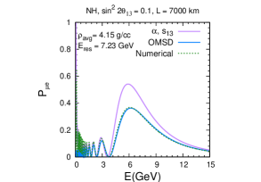
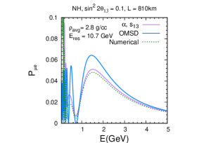
Figure 2.2: Comparison between OMSD and $\alpha-s_{13}$ approximation.

As for example, in Fig. 2.2 we have plotted $P_{\mu e}$ as a function of energy for the baselines 7000 km and 810 km. From the figure we can notice that for $L=7000$ km and $E=7.23$ GeV which is the MSW region relevant for the case of the atmospheric neutrinos, the OMSD approximation matches perfectly with the numerical calculation . On the other hand for the baseline of 810 km, where the first oscillation maximum lies very far from the resonance energy, the $\alpha-s_{13}$ approximation gives better estimation than the OMSD approximation.

2.3 Current Status of the Oscillation Parameters

In this section we discuss the current status of neutrino oscillation parameters. The mass and mixing parameters that describe the oscillation of the three generation neutrinos, are divided into three categories (except the leptonic phase $\delta_{CP}$): the solar neutrino parameters i.e., $\theta_{12}$, $\Delta_{21}$, the atmospheric neutrino parameters i.e., $\theta_{23}$, $\Delta_{31}$ and reactor neutrino parameter i.e., $\theta_{13}$. The parameters are termed like this because the oscillation in the respective sectors are governed mainly by these parameters. Specifically the parameters $\theta_{12}$ and $\Delta_{21}$ are mainly constrained from the solar neutrino experiments and KamLAND reactor data. The accelerator based long-baseline experiments (MINOS, T2K) constrain the parameters $|\Delta_{31}|$, $\theta_{23}$, and $\delta_{CP}$. The parameters $|\Delta_{31}|$ and $\theta_{23}$ are also constrained from Super-Kamiokande. The reactor data (Daya-Bay, RENO and Double-Chooz) constrain $\theta_{13}$ and $\Delta_{ee}\big{(}=s_{12}^{2}\sin^{2}(\frac{\Delta_{32}L}{4E})+c_{12}^{2}\sin^{2}(\frac{\Delta_{31}L}{4E})\big{)}$. Note that, as non-zero value of $\theta_{13}$ affects both solar and atmospheric oscillation results, it plays an important role in the global fit of world neutrino data.

At present, one of the major unknowns in the three flavour oscillation picture is the sign of the atmospheric mass squared difference $\Delta_{31}$ or the neutrino mass hierarchy. The $+$ve sign of $\Delta_{31}$ corresponds to $m_{3}>m_{1}$ which is known as normal hierarchy (NH) and $-$ve sign of $\Delta_{31}$ implies $m_{3}<m_{1}$ which is known as inverted hierarchy(IH) (shown in Fig. 2.3).

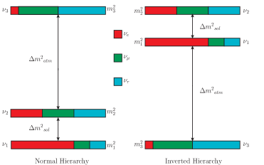
Figure 2.3: Two possible mass orderings of neutrinos.

The second unknown in this sector is the octant of $\theta_{23}$. If $\theta_{23}$ is less than $45^{\circ}$, then the octant of $\theta_{23}$ is lower (LO) and if $\theta_{23}$ is greater than $45^{\circ}$ then the octant of $\theta_{23}$ is higher (HO). The last remaining unknown in the three flavour framework is the value of the leptonic phase $\delta_{CP}$.

Next we discuss the current status of these parameters in detail. Currently there are three groups doing the global analysis of the world neutrino data. We have given the results of the latest global analysis by the Nu-fit group [124] in Table 2.1 and compared the results of different groups in Fig. 2.4 in terms of best-fit values and $3\sigma$ ranges. The blue, red and black lines correspond to the analysis by the Bari group [19], IFIC group [125] and Nu-fit group respectively. The solid (dashed) line corresponds to NH (IH).

parameter	present value	precision
$\frac{\Delta m^{2}_{21}}{10^{-5}~{}\mathrm{eV}^{2}}$	7.50${}^{+0.19}_{-0.17}$	2.3%
$\sin^{2}\theta_{12}$	$0.304^{+0.012}_{-0.012}$	4%
$\frac{|\Delta m^{2}_{31}|}{[10^{-3}~{}\mathrm{eV}^{2}}$	+2.458${}^{+0.002}_{-0.002}$	2%
$\frac{|\Delta m^{2}_{32}|}{[10^{-3}~{}\mathrm{eV}^{2}}$	-2.458${}^{+0.002}_{-0.002}$	2%
$\sin^{2}\theta_{23}$	0.451${}^{+0.001}_{-0.001}\oplus 0.577^{+0.027}_{-0.035}$	7.5%
$\sin^{2}\theta_{13}$	$0.0219^{+0.0010}_{-0.0011}$	5%
$\delta_{CP}$	$0.80\pi$ (NH) $-0.03\pi$ (IH)	$0-2\pi$

Table 2.1: The best-fit values and $3\sigma$ ranges of neutrino oscillation parameters from global analysis by the Nu-fit group [124].

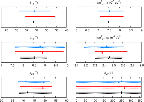
Figure 2.4: Comparison of the best-fit values and $3\sigma$ ranges of the oscillation parameters. The figure is taken from Ref. [126].

From Fig. 2.4 we can see that except $\theta_{23}$, the global analysis results for the other parameters, are consistent among the three groups. For the mixing angles, best-fit values of $\theta_{12}$ and $\theta_{13}$ are around $34^{\circ}$ and just below $9^{\circ}$ respectively. For mass squared differences, the best-fit values of $\Delta_{21}$ and $|\Delta_{31}|$ come around $7.5\times 10^{-5}$ eV² and $2.4\times 10^{-3}$ eV² respectively. The analysis also shows that, at this moment both the hierarchies give equally good fit to the data. Regarding the phase $\delta_{CP}$, we can see that the current data signal a best-fit value around $250^{\circ}$. This hint is mainly driven by the T2K appearance channel measurement and data from the reactors measuring $\theta_{13}$. But this signal is not statistically significant as at $3\sigma$, the full $\delta_{CP}$ range becomes allowed.

Now let us discuss the case of $\theta_{23}$ in detail. In their analysis, the Bari group has fitted $\theta_{23}$ separately for NH and IH. When the data from long-baseline, solar and KamLAND are combined, they get the best-fit of $\theta_{23}$ in the higher octant for both NH and IH. But after addition of the reactor data, whose main effect is to reduce the $\theta_{13}$ uncertainty, the best-fit for NH shifts to the lower octant. The conclusions after adding the Super-Kamiokande atmospheric data are different before and after the Neutrino 2014 conference. Before Neutrino 2014, due to the addition of the Super-Kamiokande data, the best-fit for IH shifted to the lower octant but after Neutrino 2014 addition of Super-Kamiokande data only increases the significance of the fit for the lower octant in NH and for IH the best-fit remains in the higher octant [126]. Thus according to results from the global analysis by the Bari group, $\theta_{23}$ seems to prefer the LO for NH and and HO for IH. This result is different with their previous analysis result [127], where for both the hierarchy best-fit was obtained in the lower octant. But the conclusions are somewhat different according to the analysis of IFIC group, which also do separate fits for NH and IH. From the analysis of the solar, KamLAND and accelerator data, they found the best-fit to come in the lower octant for both NH and IH. By the addition of reactor data, the best-fit values for both the hierarchies move to the higher octant. In this case the addition of Super-Kamiokande data do not have any effect. Thus the analysis of IFIC group shows that $\theta_{23}$ prefers HO for both the hierarchies. Now let us come to the results of Nu-fit group. The Nu-fit group does not analyse NH and IH separately. In their analysis they get the global best-fit of $\theta_{23}$ in the higher octant and for IH. For NH, a local minima is obtained. So in conclusion we can say that, from the present available information of the world neutrino data, there is yet no clear hint about the octant of $\theta_{23}$ and more data from present/future experiments are expected to address this issue.

Now let us discuss a bit more about of the present unknowns in terms of oscillation probabilities.

• As discussed earlier, matter effect plays a key role in the determination of neutrino mass hierarchy. Note that for the solar neutrinos, the MSW resonance effect in the core of the Sun implies that the solar mixing angle $\theta_{12}$ is in the first octant and this gives $m_{2}>m_{1}$ [128]. For the determination of the sign of $\Delta_{31}$, one needs to study the Earth matter effect of neutrino oscillation. In Table 2.2, we list the resonance energies for different baselines in the Earth as given in [129]. From these we understand that the energies of the current generation long-baseline experiments are very far from the resonance energies to observe the MSW resonance effect. But still these experiments can have hierarchy sensitivity coming from the electron neutrino appearance channel depending on the length of the baseline. At present T2K and NO$\nu$A are the examples of such long-baseline experiments which have given data corresponding to appearance channel. But the comparatively smaller baseline of T2K does not allow it to measure neutrino mass hierarchy and the first results from NO$\nu$A [54] are also not yet statistically significant for getting a clear hint. On the other hand the atmospheric neutrino experiments study the oscillation of the neutrinos having energy ranging from 1-10 GeV with the maximum available baseline equals to the diameter of the Earth. So it is possible to determine neutrino mass hierarchy in the atmospheric neutrino experiments via MSW resonance effect in both appearance and disappearance channel . But for the current Super-Kamiokande experiment, at this moment there is not enough statistics for obtaining any clear hint about the true mass hierarchy.

  Baseline(Km)	Resonance Energy (GeV)
  3000	9.4
  5000	8.7
  7000	7.5
  10000	6.6

  Table 2.2: Resonance energies at different baselines assuming average PREM density profile as calculated in [129].

• Now let us discuss why the octant of $\theta_{23}$ is still unknown. Similar to that of hierarchy, the octant sensitivity of the long-baseline experiments come from only appearance channel (cf. Eqs. 2.101 and 2.2.5) and in the atmospheric experiments octant sensitivity arise from both appearance and disappearance channel (cf. Eqs. 2.75 and 2.2.4). From the probability expressions in matter, we see that the leading order term of the appearance channel depends on $\sin^{2}\theta_{23}$ and thus the appearance channel probability is an increasing function of $\theta_{23}$. But in the disappearance channel probability, the leading order term $\sin^{2}2\theta_{23}$ gives equal probability for $\theta_{23}$ and $\pi/2-\theta_{23}$. But note that, though the disappearance channel do not give any octant sensitivity for the long-baseline experiments but this channel is useful for the precision measurement of $\theta_{23}$. Thus in principle it is possible to determine the octant of $\theta_{23}$ from the combination of appearance and disappearance channels in the long-baseline experiments if $\theta_{23}$ is not very close to maximal. On the other hand, for atmospheric neutrinos, due to matter effect, the disappearance channel also contribute in the octant measurement. But at present the available statistics is not enough to predict the correct octant of $\theta_{23}$.

• In the previous section we have seen that under OMSD approximation the conversion probability for $\nu_{e}$ do not involve $\delta_{CP}$ and in the $\alpha-s_{13}$ approximation, $\delta_{CP}$ appears in the sub leading term $\alpha$. So we understand that $\delta_{CP}$ is a sub-leading effect in neutrino oscillation and thus it is the most difficult parameter to probe in the experiments. Though the atmospheric neutrino experiments can have CP sensitivity in principle but they are not expected to measure $\delta_{CP}$ as we will show in the next chapter that their CP sensitivity is compromised due to their dependence on the direction of the incoming neutrinos. On the other hand as reactor experiments are sensitive only to electron appearance channel which do not depend on $\delta_{CP}$, they are also not capable of measuring this parameter. So it is expected that the first hint of $\delta_{CP}$ will come from the appearance channel measurement of the long-baseline experiments. As we have already discussed, the current T2K data gives a hint of $\delta_{CP}$ about ($-90^{\circ}$), but this needs to be confirmed from the further runs of T2K as well as data from future experiments.

Apart from the reasons mentioned above, the measurement of these above unknowns are also restricted due to the presence of parameter degeneracy, which we will discuss now.

2.4 Degeneracies in Oscillation Parameters

In this section we will discuss the degeneracies between the different oscillation parameters. The parameter degeneracy in the context of neutrino oscillations implies getting the same value of probability for different sets of oscillation parameters. The sensitivity of an experiment depends on the number of events which are the functions of neutrino oscillation probabilities. This implies that in the presence of degeneracies, different sets of parameters can give equally good fit to the data making it difficult to determine the actual values of the parameters unambiguously. So a clear understanding of various degeneracies, their dependence on different oscillation parameters and their resolution are very important for the determination of the unknown parameters. Previously when $\theta_{13}$ was unknown, three types of degeneracies have been discussed widely in the literature: (i) the intrinsic ($\theta_{13}$, $\delta_{CP}$) degeneracy [131], (ii) hierarchy-$\delta_{CP}$ degeneracy [132], and (iii) the degeneracy of octant of $\theta_{23}$ [133]. The intrinsic degeneracy of the $P_{\mu e}$ channel refers to the same value of probability coming from a different $\theta_{13}$ and $\delta_{CP}$ value and can be expressed as

$$P_{\mu e}(\theta_{13},\delta_{CP})=P_{\mu e}(\theta_{13}^{\prime},\delta_{CP}^{\prime}).$$ (2.105)

The hierarchy-$\delta_{CP}$ degeneracy of the $P_{\mu e}$ channel leads to wrong hierarchy solutions arising due to a different value of $\delta_{CP}$ other than the true value. This degeneracy can be expressed mathematically as

$$P_{\mu e}(\text{NH},\delta_{CP})=P_{\mu e}(\text{IH},\delta_{CP}^{\prime}).$$ (2.106)

The intrinsic octant degeneracy of the $P_{\mu\mu}$ channel refers to the clone solutions occurring for $\theta_{23}$ and $\pi/2-\theta_{23}$ and expressed as

$$P_{\mu\mu}(\theta_{23})=P_{\mu\mu}(\pi/2-\theta_{23}).$$ (2.107)

These above mentioned degeneracies together (Eqs. 2.105, 2.106 and 2.107) gave rise to a total eight fold degeneracy [134]. It is important to note that there is no intrinsic octant degeneracy in the $P_{\mu e}$ channel as the dependence of $\theta_{23}$ in the leading order term of $P_{\mu e}$ channel goes as $\sin^{2}\theta_{13}\sin^{2}\theta_{23}$. But due to the presence of the $\sin^{2}\theta_{13}$ term, continuous allowed regions were obtained in the $\theta_{13}-\theta_{23}$ plane for a given value of $\delta_{CP}$ when $\theta_{13}$ was not known very precisely. There were several proposals on how to break these degeneracies to have a clean measurement of the neutrino oscillation parameters [135, 136, 137, 138, 139, 140, 141, 142, 143, 144, 145, 146]. It is shown that the intrinsic degeneracy can be removed to a large extent by using spectral information [140]. At present, the measurement of the non-zero precise value of $\theta_{13}$ from the reactor experiments resolves the degeneracies associated with $\theta_{13}$. The intrinsic degeneracy is largely resolved and the octant sensitivity of the appearance channel has greatly improved. But due to the completely unknown value of $\delta_{CP}$, the hierarchy-$\delta_{CP}$ degeneracy still persists and there are also degenerate solutions arising due to different values of $\theta_{23}$ and $\delta_{CP}$. This degeneracy is referred as octant-$\delta_{CP}$ degeneracy [147]. We will now discuss the behaviour of these degeneracies in detail in the next subsections.

2.4.1 The Hierarchy-$\delta_{CP}$ Degeneracy

As discussed above the hierarchy-$\delta_{CP}$ degeneracy of the appearance channel is defined by

$$P_{\mu e}(\text{NH},\delta_{CP})=P_{\mu e}(\text{IH},\delta_{CP}^{\prime}),$$ (2.108)

i.e., for a given octant, the probability for NH can be the same as that of probability for IH, for a different value of $\delta_{CP}$. To understand this degeneracy, in Fig. 2.5 we have plotted the appearance channel probability vs energy for a baseline of 812 km. At this baseline the constant matter density approximation holds good and we can use Eq. 2.101 to understand the behaviour of Fig. 2.5. The left panel in Fig. 2.5 is for neutrinos and the right panel corresponds to antineutrinos. In this plot $\theta_{23}$ is fixed at $39^{\circ}$. The blue band corresponds to NH and the red band corresponds to IH. Here the values of $\Delta_{31}$ are taken as $2.4(-2.4)\times 10^{-3}$ eV² corresponding to NH (IH). The width of the bands is due to the variation of $\delta_{CP}$ from $-180^{\circ}$ to $+180^{\circ}$. As matter effect enhances the neutrino probability for NH and antineutrino probability for IH, in these plots we see that for the neutrinos, NH probability is higher than IH and for the antineutrinos, IH probability is higher than NH. In the neutrino probability, we observe that for each band (either NH or IH) $\delta_{CP}=-90^{\circ}$ corresponds to the highest point in the probability and $\delta_{CP}=90^{\circ}$ is the lowest point in the probability. This behaviour is opposite for the antineutrinos. This can be understood by having a close look at the Eq. 2.101.

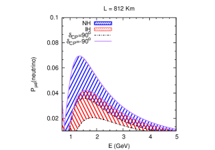
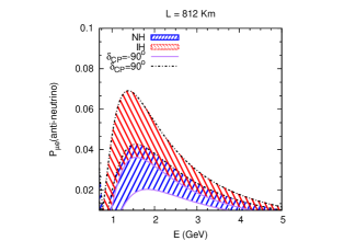
Figure 2.5: $P_{\mu e}$ vs energy for L=812 km. The blue band corresponds to NH and the red band corresponds to IH.

At the oscillation maximum, $\Delta=90^{\circ}$. Thus the $\delta_{CP}$ dependent term for neutrinos becomes maximum for $\delta_{CP}=-90^{\circ}$ and minimum for $\delta_{CP}=90^{\circ}$. For antineutrinos as $\delta_{CP}$ changes its sign this behaviour gets reversed. In both the plots we observe that there is an overlap between the NH band at $\delta_{CP}=+90^{\circ}$ and IH band at $\delta_{CP}=-90^{\circ}$. If the true values of the parameters fall in the overlapping region then we will have degenerate solutions. Based upon this observation if we divide the total range of $\delta_{CP}$ into two half-planes i.e., the lower half-plane (LHP: $-180^{\circ}<\delta_{CP}<0^{\circ}$) and upper half-plane (UHP: $0^{\circ}<\delta_{CP}<180^{\circ}$), then we see that the combination of hierarchy and $\delta_{CP}$ given by NH-LHP and IH-UHP lies far away from the overlapping regions. Hence these combinations do not suffer from the hierarchy-$\delta_{CP}$ degeneracy and thus LHP (UHP) is the favourable half-plane for NH (IH). On the other hand the combination of NH-UHP and IH-LHP lies very close to the overlapping area and hence can give rise to hierarchy-$\delta_{CP}$ degeneracy. Thus UHP (LHP) is the unfavourable half-plane for NH (IH) in view of this degeneracy. Here it is important to note that the favourable and unfavourable half-planes remain same in both neutrinos and antineutrinos.

One of the ways to overcome the hierarchy-$\delta_{CP}$ degeneracy is to look for neutrino oscillations at higher baselines. At longer baselines, there will be more matter enhancement of the oscillation probabilities and this will cause more separation between the NH and IH bands. This is shown in Fig. 2.6, where we can see that near the oscillation maxima, there is no overlap between the NH and IH bands for the 1300 km baseline.

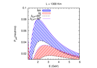
Figure 2.6: Similar plot as that of Fig. 2.5 but for 1300 km baseline.

Another elegant method to get rid of this degeneracy is the following: If one puts $\sin^{2}\hat{A}\Delta=0$ in Eq. 2.101, then the probability expression becomes free from the $\delta_{CP}$ term and thus there is no hierarchy-$\delta_{CP}$ degeneracy. This condition translates to $L=7690$ km for both NH and IH and this baseline is referred as the magic baseline [148]. This is reflected in Fig. 2.7, where one can see that for $L=7690$ km, the hierarchy-$\delta_{CP}$ degeneracy is completely absent. One also notices that, the width of the $\delta_{CP}$ band is very narrow.

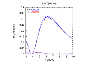
Figure 2.7: Similar plot as that of Fig. 2.5 but for 7690 km baseline.

In spite of having this magical property, practically it is a very difficult task to design a neutrino oscillation experiment for a baseline of 7690 km. As the flux of the neutrinos fall as $1/L^{2}$, one needs a very powerful collimated neutrino beam to have enough statistics at such a large distance . Another problem with the magic baseline is that, it has no CP sensitivity. These problems lead to the question that can there be a shorter baseline where the hierarchy-$\delta_{CP}$ degeneracy can be removed and at the same time one can also have CP sensitivity. These questions were answered in [151] by observing that if one puts $\sin^{2}(\hat{A}-1)=0$ in Eq. 2.101, then also the CP sensitive term goes to zero. Unlike the magic baseline, this condition also depends on hierarchy. If we now demand that there is no $\delta_{CP}$ dependence for IH and at the same time there is a probability maxima in NH, then one gets the following conditions

$$(1+\hat{A}) > n\pi~{}~{}{\rm for}~{}~{}n>0,$$ (2.109)

$$(1-\hat{A}) > (m-1/2)\pi~{}~{}{\rm for}~{}~{}m>0.$$

Solving these two equations simultaneously one obtain $L\approx 2540$ km and $E\approx 3.3$ GeV for $n=m=1$. Now on the other hand if one demands that there will be no $\delta_{CP}$ dependence for NH and a probability maxima in IH, then one obtains [152]

$$(1-\hat{A}) > n\pi~{}~{}{\rm for}~{}~{}n>0,$$ (2.110)

$$(1+\hat{A}) > (m-1/2)\pi~{}~{}{\rm for}~{}~{}m>0,$$

and solutions of these two equations again yield $L\approx 2540$ km but $E\approx 1.9$ GeV for $n=1$, $m=2$. These features are shown in Fig. 2.8, where one can see that for $L=2540$ km there is no CP sensitivity in IH and probability maxima in NH at $E=3.3$ GeV and at $E=1.9$ GeV there is no CP sensitivity in NH and probability maxima in IH.

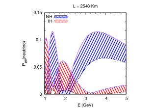
Figure 2.8: Similar plot as that of Fig. 2.5 but for 2540 km baseline.

Thus for a baseline of $L=2540$ km, one can have hierarchy sensitivity for both NH and IH with CP dependence in one hierarchy and with no CP dependence for the opposite hierarchy though at different energies. This baseline was termed as the bi-magic baseline [151, 153, 152]. In the next chapter, while discussing the physics potential of the LBNO experiment we will see that there is an exceptional hierarchy sensitivity at the CERN-Pyhäsalmi baseline of $L=2290$ km due to its proximity to the bi-magic baseline.

Note that in the atmospheric neutrinos experiments, oscillation takes place over the baselines ranging from 100 km to 12000 km experiencing huge Earth matter effects. For this reason the effect of hierarchy-$\delta_{CP}$ degeneracy is less pronounced for the case of atmospheric neutrinos.

2.4.2 The Octant-$\delta_{CP}$ Degeneracy

The octant-$\delta_{CP}$ degeneracy can be expressed mathematically in the following way

$$P_{\mu e}(\text{LO},\delta_{CP})=P_{\mu e}(\text{HO},\delta_{CP}^{\prime}),$$ (2.111)

i.e., for a given hierarchy, the appearance channel probability for lower octant can be the same as the probability for the higher octant corresponding to a different value of $\delta_{CP}$. To understand how this degeneracy behaves in neutrino and antineutrino probabilities, in Fig. 2.9, we show the appearance channel probability as a function of energy by fixing the hierarchy to be NH. This figure corresponds to a baseline of 812 km. The left panel is for neutrinos and the right panel is for antineutrinos. The blue band corresponds to LO and red band corresponds to HO. In these plots LO (HO) corresponds to $\theta_{23}=39^{\circ}(51^{\circ})$. Here also the width of the bands are due to the variation of $\delta_{CP}$ from $-180^{\circ}$ to $+180^{\circ}$. As the leading order term in the oscillation probability depends on $\sin^{2}\theta_{23}$, we see that for both neutrinos and antineutrinos, the probability for HO is higher than LO. As discussed earlier, for neutrinos, in each band, $\delta_{CP}=-90^{\circ}$ corresponds to maximum point in the probability and $\delta_{CP}=90^{\circ}$ corresponds to the minimum point in the probability while opposite is true for antineutrinos.

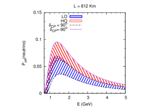
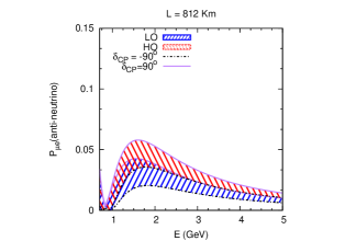
Figure 2.9: $P_{\mu e}$ vs energy for L=812 km. The blue band corresponds to LO and the red band corresponds to HO.

Now from the probability figure we observe that, for neutrinos the overlap is around LO-$\delta_{CP}=-90^{\circ}$ and HO-$\delta_{CP}=90^{\circ}$ and for antineutrinos the overlap is around LO-$\delta_{CP}=90^{\circ}$ and HO-$\delta_{CP}=-90^{\circ}$. So in this case for neutrinos, UHP (LHP) is the favourable half-planes for LO (HO), where it is less probable to have the octant-$\delta_{CP}$ degeneracy and LHP (UHP) is the unfavourable half-planes for LO (HO) where one has the octant-$\delta_{CP}$ degeneracy. But this situation gets reversed in the antineutrinos i.e., the favourable regions for neutrinos become unfavourable in antineutrinos and the unfavourable regions for neutrino become favourable in antineutrinos. This is the main difference between the hierarchy-$\delta_{CP}$ and octant-$\delta_{CP}$ degeneracy, where in the former case, the data from antineutrinos do not help to resolve this degeneracy but for the later case, it is possible to resolve this degeneracy with balanced neutrino and antineutrino runs.

Here we would like to mention that as the atmospheric neutrinos consists of both neutrinos and antineutrinos, the octant-$\delta_{CP}$ degeneracy is less for the case of atmospheric neutrino experiments. In this case the sub-leading terms of the disappearance channel also provide octant sensitivity due to large matter effects. In this context it is important to note that in the atmospheric neutrinos the uncertainty in $\theta_{13}$ do not affect the measurement of $\theta_{23}$. This is because near the resonance region the $\sin^{2}2\theta_{13}^{M}$ term in Eq. 2.2.4 becomes unity.

From the above discussions we understand how the presence of hierarchy-$\delta_{CP}$ and octant-$\delta_{CP}$ degeneracy, can severely affect the determination of the unknown oscillation parameters. The hierarchy-$\delta_{CP}$ degeneracy gives rise to wrong hierarchy solutions, whereas octant-$\delta_{CP}$ gives rise to wrong octant solutions. These two types of degeneracies together give rise to a generalised hierarchy-$\theta_{23}$-$\delta_{CP}$ degeneracy defined as

$$P_{\mu e}({\rm NH},\theta_{23},\delta_{CP})=P_{\mu e}({\rm IH},\theta_{23}^{\prime},\delta_{CP}^{\prime}),$$ (2.112)

which can give wrong hierarchy-wrong octant solution. As hierarchy, octant and $\delta_{CP}$ are interlinked, the determination of one quantity depends on the information of the other quantities and the presence of degeneracies makes it difficult to extract the correct information as the true solution can often be faked by other degenerate solutions. In [147, 154] it was shown that the hierarchy and octant sensitivity of the long-baseline experiments suffers from these above mentioned degeneracies due to the unknown value of $\delta_{CP}$. In the next chapter when we will study the physics potential of the various oscillation experiments, we will show how the lack of knowledge of hierarchy and octant, affect the CP measurement capabilities of the long-baseline experiments.

2.5 Salient Features of the Present/Future Generation Oscillation Experiments

In this section we discuss the main features of the currently running/upcoming oscillation experiments T2K, NO$\nu$A, LBNO, LBNE and INO which are expected to throw light on the three yet undetermined parameters of neutrino oscillation. We will also briefly describe the IceCube experiment at south pole. Though the aim of the IceCube experiment is to study the physical processes associated with the ultra high energy neutrinos of astrophysical origin, but one can also put constraint on the various oscillation parameters by analysing its data. These are the experiments whose potentials have been studied in this thesis for determination of neutrino mass hierarchy, octant of $\theta_{23}$ and the leptonic CP phase $\delta_{CP}$.

2.5.1 T2K

T2K (Tokai to Kamioka) is a long-baseline experiment in Japan looking for neutrino oscillations in both appearance and disappearance channels [155]. T2K uses Super-Kamiokande (SK) as the far detector, which is a water Čerenkov detector located in the Kamioka Observatory, Gifu, Japan, at a distance of 295 km from J-PARC high-intensity proton accelerator. The beam power is 0.75 MW with mean neutrino energy as 0.76 GeV. The neutrino beam is directed 2.5 degrees off-axis from the SK detector, in order to produce a narrow-band flux at 0.6 GeV. The experiment also includes two near detectors at a distance 280 m (INGRID and ND280). Construction of the neutrino beamline started in April 2004. After successful installation of the accelerator and neutrino beamline in 2009, T2K began accumulating neutrino beam data for physics analysis in January 2010. But it was interrupted for one year due to the Great East Japan Earthquake in 2011. Up to now T2K has collected data corresponding to the exposure of $6.6\times 10^{20}$ POT (Protons on Target) in neutrino mode and currently taking data in antineutrino mode. The recent measurements of the oscillation parameters in T2K can be found in [53]. We summarize the details of data taking of T2K in Table 2.3.

Run Period	Dates	POT
Run 1	Jan. 2010 - Jun. 2010	$0.32\times 10^{20}$
Run 2	Nov. 2010 - Mar. 2011	$1.11\times 10^{20}$
Run 3	Mar. 2012 - Jun. 2012	$1.58\times 10^{20}$
Run 4	Oct. 2102 - May 2013	$3.56\times 10^{20}$
Total	Jan. 2010 - May 2013	$6.57\times 10^{20}$

Table 2.3: The data taking period of T2K in neutrino mode as given in [53].

2.5.2 NO$\nu$A

The NuMI Off-axis $\nu_{e}$ Appearance (NO$\nu$A) experiment at Fermilab is a two-detector, long-baseline, neutrino oscillation experiment optimised for $\nu_{e}$ identification. NO$\nu$A uses Fermilab’s NuMI beamline having a beam power of 700 KW, as its neutrino source. The 14 kt far detector is situated at a distance of 812 km, near Ash River, Minnesota and the 0.3 kt near detector is located at the Fermilab site, near the existing MINOS Near Detector Hall. The 14 mrad off-axis configuration of the NuMI beam gives relatively narrow band of neutrino energies centered at 2 GeV. Both the NO$\nu$A detectors are highly segmented, highly active tracking calorimeters, filled with liquid scintillator. NO$\nu$A has started taking data from December 2014 and has given the first physics results recently [54]. More details of NO$\nu$A has been discussed in [89].

2.5.3 LBNO

One of the promising proposals for long-baseline neutrino oscillation experiment, is the LAGUNA (Large Apparatus studying Grand Unification and Neutrino Astrophysics) -LBNO (Long Baseline Neutrino Oscillation) project in Europe [92]. The source of neutrinos for this experiment is likely to be at CERN. Various potential sites for the detector have been identified by LAGUNA, including Boulby (U.K.), Canfranc (Spain), Fréjus (France), Pyhäsalmi (Finland), Slanic (Romania), SUNLAB (Poland) and Umbria (Italy) [157]. There are three different proposed detectors for the LBNO project: GLACIER (liquid argon), LENA (liquid scintillator) and MEMPHYS (water Čerenkov). In 2011, The LAGUNA collaboration decided to go ahead to investigate three sites in detail: Fréjus having the shortest baseline of 130 km, Pyhäsalmi with the longest baseline (2300 km) and Slanic having baseline of 1500 km. The corresponding detector for Pyhäsalmi and Slanic is GLACIER and for Fréjus is MEMPHYS. To produce the beam for the Fréjus (130 km) configuration, the 4 MW, 5 GeV HP-SPL proton driver was assumed. For the other baselines, the 1.6 MW, 50 GeV HP-PS was considered. For a operation of 200 days per calendar year, the HP-SPL delivers $10^{21}$ POT and the HP-PS yields integrated $3\times 10^{21}$ POT per year. In the past years, study regarding the beam optimisation, detector simulation and physics potential at the various baselines has been carried out in great detail. The details of the physics simulation of LBNO can be found in [158, 159].

2.5.4 LBNE

The Long Baseline Neutrino Experiment (LBNE) is a proposed long-baseline experiment at Fermilab [91]. The proposed detector is a modular 40 kt Liquid Argon Time Projection Chamber (LArTPC) at Sanford Underground Research Facility (SURF) in South Dakota at a distance 1300 km from the source. The first phase of this will be a 10 kt detector. There will also be a fine-grained ‘near’ neutrino detector. Performance of LArTPC is unmatched among massive detectors for precise spatial and energy resolution and for reconstruction of complex neutrino interactions with high efficiency over a broad energy range. It thus provides a “compact, scalable” approach to achieve sensitivity to the oscillation physics goals of LBNE [160]. If the LBNE detector is built underground, it will also be possible for it to observe atmospheric neutrinos. A detailed study on atmospheric neutrinos at LBNE is presented in [161, 162]. The beam of LBNE will have a intense on-axis wide-band profile with a beam power of 1.2 GeV. There are two options being considered for the proton beam – 80 GeV and 120 GeV. For a given beam power, proton energy varies inversely with the number of protons in the beam per unit time. Thus a higher proton energy implies a lower flux of neutrinos.

Recently there have been discussions to converge the expertise and technical knowledge of LBNO and LBNE into a unified endeavor of a long-baseline experiment named DUNE (Deep Underground Neutrino Experiment) using a Megawatt beam from Fermilab. One of the major goals of this facility as outlined in [90] is $3\sigma$ CP sensitivity for 75$\%$ values of $\delta_{CP}$.

2.5.5 INO

The India-based neutrino observatory (INO) project is a multi-institutional effort aimed at building a world-class underground laboratory in India for studying atmospheric neutrinos in its first phase [95]. It is sensitive to the atmospheric neutrinos in the energy range of 1-10 GeV. For this experiment, the detector will be 50 kt magnetised iron calorimeter (ICAL) which is sensitive to mainly muon events. ICAL will consist of 5.6 m thick iron plates sandwiched between 151 layers of Resistive Plate Chambers (RPCs). Iron will act as a target and the RPCs will serve as the active detector elements. Due to the magnetic field of strength 1.5 Tesla, ICAL will be able to distinguish the $\mu^{+}$ and $\mu^{-}$ events in the GeV energy range. This will make the ICAL detector sensitive towards measuring the neutrino mass hierarchy, which is the primary goal of the ICAL@INO experiment. Analysis of hierarchy sensitivity of the ICAL detector using only the muon momentum information can be found in [164]. It is also capable of reconstructing the hadron energy and average direction of hadron shower. The improvement in the sensitivity due to the inclusion of hadrons is discussed in [165]. Apart from determining the neutrino mass hierarchy, the other physics goals of the ICAL@INO experiment include measurement of octant of $\theta_{23}$, indirect detection of dark matter, searches for magnetic monopoles, non standard interactions, Lorentz and CPT violation etc. The site for the INO has been identified at Pottipuram in Bodi West hills of Theni District of Tamil Nadu and the construction is expected to start soon.

2.5.6 IceCube

The IceCube Neutrino Observatory is a neutrino telescope constructed at the Amundsen-Scott South Pole Station in Antarctica. The main aim of IceCube is to study neutrinos from astrophysical sources. IceCube consists of 4800 optical sensors installed on 80 strings between 1450 m and 2450 m below the surface. Strings are deployed in a triangular grid pattern with a characteristic spacing of 125 m enclosing an area of 1 km² [166]. The IceCube telescope was deployed in the summer of 2004 and is taking data since 2005. But the evidence of extraterrestrial neutrinos are found just recently. IceCube observed 37 neutrino candidate events in the energy range 30 TeV to 2000 TeV [167]. The data in this energy range can be explained by an $E^{-2}$ neutrino spectrum with a per-flavour normalisation (1:1:1). On 4th august 2015 IceCube has observed a 2.3 PeV neutrino event [76] which corresponds to the highest energy neutrino ever detected.

Chapter 3   Probing Neutrino Oscillation Parameters in Future Experiments

3.1 Overview

In this chapter we will study the sensitivity reach of the present/future generation experiments for determining the remaining unknown neutrino oscillation parameters, namely: (i) the neutrino mass hierarchy, (ii) the octant of the mixing angle $\theta_{23}$ and (iii) the leptonic CP phase $\delta_{CP}$. We will analyse the sensitivities of the current long-baseline experiments T2K and NO$\nu$A, future atmospheric experiment ICAL@INO and the proposed long-baseline experiments LBNO and LBNE. We will also analyse the recent data of the IceCube experiment in this context. This chapter is organised in the following way. In the Section 3.2 we will study the CP sensitivity of the T2K, NO$\nu$A and ICAL experiments. Taking the projected exposures of T2K and NO$\nu$A  we will show that the combined CP sensitivity of T2K and NO$\nu$A is limited due to the presence of parameter degeneracies and we will demonstrate how ICAL@INO can be used as a remedy of this problem. Next we will explore the CP sensitivity reach of these setups by taking combinations of different exposures. We will present our results in terms of both discovery of CP violation (CPV) and precision of $\delta_{CP}$. We will also study dependence of CP sensitivity on different oscillation parameters and compare the sensitivities of T2K and NO$\nu$A for a given exposure. As the sensitivity of NO$\nu$A and T2K is limited due to shorter baselines and less statistics, it is necessary to study neutrino oscillations at higher baseline with higher statistics. In Section 3.3 and 3.4 we will study the potential of the proposed long-baseline experiments LBNO and LBNE respectively for determining all the three above-mentioned unknowns. These experiments have longer baselines as compared to T2K and NO$\nu$A and due to huge detector volume and high beam power they have higher statistics. As the exact configurations of these experiments are not yet decided, it is very important to find an optimal and economised configuration for LBNO and LBNE. It is also important to remember that when these experiments will be operational, the data from T2K, NO$\nu$A and ICAL experiments will also be available. Thus, in our analysis, we have calculated the minimum exposures of LBNO and LBNE for determining hierarchy, octant and CP violation at a given confidence level in conjunction with T2K, NO$\nu$A and ICAL. We will show that due to the synergy between T2K, NO$\nu$A and ICAL, the required exposures of the LBNO and LBNE experiments are reduced significantly. The reduction of the exposure signifies the fact that the same physics sensitivity can be obtained with a lower beam power, small detector mass and/or less runtime. For the LBNE experiment, we will also present results showing the effect of adding a near detector, the role of the second oscillation maximum and that of antineutrino runs. We will show that addition of a near detector reduces the systematic error significantly, whereas the second maxima plays a non-trivial role only in the determination of hierarchy. While studying the role of the antineutrinos we find that the combination of equal neutrino and antineutrino do not always gives the best result. In Section 3.5 of this chapter we will study the CP sensitivity of the IceCube experiment. As we have discussed in the Chapter 1, the IceCube experiment at south pole is designed mainly for studying neutrinos from astrophysical sources. While coming from the extragalactic sources, ultra high energy neutrinos oscillate and due to the very large distance, their mass dependent oscillatory terms average out and they have no explicit dependence on the oscillation probabilities. Thus in principle it is possible to probe the mixing parameters in the IceCube events irrespective of the value of the neutrino mass. In our analysis, we have investigated the possibility of constraining the leptonic phase $\delta_{CP}$ from the recent IceCube data. We show that in the oscillations of the ultra high energy neutrinos $\delta_{CP}$ have a very weak dependence and thus it is not possible to put any constraint on $\delta_{CP}$ with significant confidence level. But we found that the results significantly depend on the initial sources of the neutrinos. We will present the results showing how the properties of different sources can be constrained from this data. Finally we will summarize all the results of this chapter in Section 3.6.

3.2 Evidence for Leptonic CP Phase from NO$\nu$A, T2K and ICAL

In this section, we study the potential for measuring CP phase $\delta_{CP}$ in the current generation long-baseline experiments T2K, NO$\nu$A and the atmospheric neutrino oscillation experiment ICAL@INO. In the PMNS matrix, $\delta_{CP}$ is associated with $\theta_{13}$. Thus a non-zero $\theta_{13}$ is required for any measurement of $\delta_{CP}$. The $10\sigma$ signature for non-zero $\theta_{13}$ leads naturally to the question to what extent CPV discovery is possible by the current superbeam experiments T2K and NO$\nu$A and/or with how much precision a true value of $\delta_{CP}$ can be measured. In these experiments, the sensitivity to $\delta_{CP}$ comes mainly from the $\nu_{\mu}-\nu_{e}$ (and $\overline{\nu}_{\mu}-\overline{\nu}_{e}$) oscillation probability, $P_{\mu e}$ ($\bar{P}_{\mu e}$) which are sensitive to $\delta_{CP}$. But as discussed in Chapter 2, the measurement of any oscillation parameter is difficult due to the presence of parameter degeneracies as the correct signal can also be faked by a wrong solutions due to hierarchy-$\delta_{CP}$ and octant-$\delta_{CP}$ degeneracy. In [154], it was shown that a prior knowledge of the hierarchy facilitates the measurement of $\delta_{CP}$ by NO$\nu$A and T2K. However, the determination of the hierarchy by NO$\nu$A and T2K itself suffers from being dependent on the ‘true’ value of $\delta_{CP}$ in nature. For the favourable combinations ({$\delta_{CP}\in[-180^{\circ},0^{\circ}]$, NH} or {$\delta_{CP}\in[0^{\circ},180^{\circ}]$, IH}), NO$\nu$A and T2K will be able to determine the hierarchy at 90% C.L. with their planned runs. But their hierarchy determination ability and hence their CP sensitivity will be poor if nature has chosen the unfavourable combinations [168]. The octant determination capability of T2K and NO$\nu$A are also affected due to the completely unknown value of $\delta_{CP}$ [147]. For the case of neutrinos, $\delta_{CP}\in[-180^{\circ},0^{\circ}]$ is the favourable (unfavourable) half-plane for determination of octant if $\theta_{23}$ belongs in HO (LO) and $\delta_{CP}\in[0^{\circ},180^{\circ}]$ is the favourable (unfavourable) half-plane for determination of octant if $\theta_{23}$ belongs to LO (HO). This is opposite for the case of antineutrinos. So to have a octant sensitivity for all $\delta_{CP}$ values, a balanced neutrino and antineutrino run is required. On the other hand, the hierarchy and octant sensitivities of atmospheric neutrino experiments, for example ICAL, are independent of $\delta_{CP}$ [129, 169]. Hence, a combination of long-baseline (LBL) and atmospheric data would be able to enhance the hierarchy and octant sensitivity for the $\delta_{CP}$ values which are adverse for the LBL experiments. This can substantially improve the ability of the LBL experiments to measure $\delta_{CP}$ in the unfavourable regions of.

This section is organised as follows. First we will give the necessary experimental details of T2K, NO$\nu$A and ICAL, used in our simulations and briefly describe the the method of $\chi^{2}$ analysis. Next we present the CP sensitivity of the combined T2K and NO$\nu$A experiments by taking their projected exposures and show that the CP sensitivity of these experiments are compromised due to the hierarchy-$\delta_{CP}$ and the octant-$\delta_{CP}$ degeneracy. Next we demonstrate that, though ICAL do not have its own CP sensitivity but still the CP sensitivity of T2K and NO$\nu$A can be enhanced significantly by including ICAL data in the analysis. Then we expand our discussions by studying synergies between these setups and dependence of different oscillation parameters by taking different exposures of T2K, NO$\nu$A and ICAL.

3.2.1 Experimental Specification

For our study we simulate NO$\nu$A and T2K using the GLoBES package [123, 170, 171, 172, 155, 139, 173, 174, 175, 89, 168]. For NO$\nu$A, we have assumed a $14$ kt totally active scintillator detector (TASD) and a neutrino beam having power of $0.7$ MW. We have used a re-optimised NO$\nu$A set-up with refined event selection criteria [168, 176]. T2K is assumed to have a $22.5$ kt water Čerenkov detector and a $0.77$ MW beam. This beam power correspond to a $10^{21}$ POT per year. In our analysis we give the exposures of NO$\nu$A/T2K as a+b where a and b denote the number of years of neutrino and antineutrino running of the experiments respectively. For these experiments, we have used the systematic errors and background rejection efficiencies as used in Ref. [168, 176].

For atmospheric neutrinos we consider ICAL@INO with a proposed mass of 50 kt. The detector is capable of detecting muon events with charge identification [95]. For our analysis we use neutrino energy and angular resolutions of (10%, $10^{\circ}$) unless noted otherwise. These are representative values giving similar sensitivity as obtained in [165] using the informations of both muons and hadrons in the simulation.

Now let us discuss briefly about our treatment of systematic errors. For the ICAL experiment we have considered the following five sources of systematic errors: (i) 20% flux normalisation error, (ii) tilt error [177] which includes the effect of deviation of the atmospheric fluxes from a power law, (iii) 5% zenith angle uncertainty, (iv) 10% cross section error and (v) an overall systematic uncertainty of 5%. But for our simulation of the long-baseline experiments we have used an overall normalisation error and an overall tilt error as used in the references mentioned above. In our analysis we have implemented the systematic errors by the method of pulls [177, 178]. We will discuss this method in the appendix.

3.2.2 Details of the Simulation

In our analysis, we give the sensitivity of the experiments in terms of $\chi^{2}$. The statistical $\chi^{2}$ for a Gaussian distribution is defined as

$$\chi^{2}_{{\rm stat}}=\text{min}\frac{(N_{{\rm ex}}-N_{{\rm th}})^{2}}{N_{{\rm ex}}},$$ (3.1)

where $N_{{\rm ex}}$ and $N_{{\rm th}}$ are the number of true (corresponds to data) and test (corresponds to theory) events respectively. In our calculation we include a marginalisation over the systematic errors by the method of pulls. The resultant $\chi^{2}$ from the various experiments are then added and finally marginalised over the test parameters over their allowed $3\sigma$ range. We have added the external (projected) information on $\theta_{13}$ from the reactor experiments in the form of a prior on $\theta_{13}$:

$$\chi^{2}_{{\rm prior}}=\left(\frac{{\sin^{2}2\theta_{13}^{{{\rm tr}}}}-\sin^{2}2\theta_{13}}{\sigma(\sin^{2}2\theta_{13})}\right)^{2},$$ (3.2)

where $\sigma(\sin^{2}2\theta_{13})$ is the $1\sigma$ error of $\sin^{2}2\theta_{13}$.

For the analysis of CP sensitivity we will use two kinds of $\chi^{2}$ which are defined in the following way:

(i) The CP violation discovery $\chi^{2}$

$$\chi^{2}_{{\rm stat}}=\text{min}\frac{(N_{{\rm ex}}(\delta_{CP}^{{\rm tr}})-N_{{\rm th}}(\delta_{CP}^{{\rm test}}=0,180^{\circ}))^{2}}{N_{{\rm ex}}(\delta_{CP}^{{\rm tr}})}$$ (3.3)

which is the potential of an experiment to differentiate a true value of $\delta_{CP}$ from the CP conserving values $0^{\circ}$ and $180^{\circ}$. This is obtained by varying $\delta_{CP}$ in the true spectrum and keeping it fixed in $0^{\circ}$ and $180^{\circ}$ in the test spectrum. As expected, the CP violation discovery potential of the experiments is zero for true $\delta_{CP}=0\circ$ and $180^{\circ}$, while it is close to maximum at the maximally CP violating values $\delta_{CP}=\pm 90^{\circ}$.

(ii) The CP precision $\chi^{2}$

$$\chi^{2}_{{\rm stat}}=\text{min}\frac{(N_{{\rm ex}}(\delta_{CP}^{{\rm tr}})-N_{{\rm th}}(\delta_{CP}^{{\rm test}}))^{2}}{N_{{\rm ex}}(\delta_{CP}^{{\rm tr}})}$$ (3.4)

which describes how well an experiment can exclude the wrong $\delta_{CP}$ values other than the true values. This is obtained by varying $\delta_{CP}$ in the test spectrum over the full range $[-180^{\circ},180^{\circ})$ for each value of true $\delta_{CP}$. We will present our CP sensitivity results in the $\delta_{CP}({\rm true})-\delta_{CP}({\rm test})$ plane.

In our analysis we use the following transformations relating the effective measured values of the atmospheric parameters $\Delta_{\mu\mu}$ and $\theta_{\mu\mu}$ to their natural values $\Delta_{31}$ and $\theta_{23}$ [179, 180, 181]:

$$\sin\theta_{23}=\frac{\sin\theta_{\mu\mu}}{\cos\theta_{13}}\ ~{},$$ (3.5)

$$\Delta_{31}=\Delta_{\mu\mu}+(\cos^{2}\theta_{12}-\cos\delta\sin\theta_{13}\sin 2\theta_{12}\tan\theta_{23})\Delta_{21}\ ~{}.$$ (3.6)

The effective values $\Delta_{\mu\mu}$ and $\theta_{\mu\mu}$ correspond to parameters measured by muon disappearance experiments. It is advocated to use these values in the definitions of priors if the prior is taken from muon disappearance measurements. The corrected definition of $\theta_{\mu\mu}$ is significant due to the large measured value of $\theta_{13}$, while for $\Delta_{\mu\mu}$ the above transformation would be relevant even for small $\theta_{13}$ values. In our analysis we do not use any external priors for these parameters as the experiments themselves are sensitive to these parameters. However it is to be noted that for the effective parameters, there is an exact mass hierarchy degeneracy between $\Delta_{\mu\mu}$ and ($-\Delta_{\mu\mu}$) and an exact intrinsic octant degeneracy between $\theta_{\mu\mu}$ and ($90^{\circ}-\theta_{\mu\mu}$). Therefore use of these values in the analysis ensures that one hits the exact minima for the wrong hierarchy and wrong octant in the numerical analysis for the muon disappearance channel. Measurements with the appearance channel and the presence of matter effects can break these degeneracies. Also, the generalised octant degeneracy occurring between values of $\theta_{\mu\mu}$ in opposite octants for different values of $\theta_{13}$ and $\delta_{CP}$ is still present for the effective atmospheric mixing angle. For such cases, a fine marginalisation grid has to be used in the analysis in order to capture the $\chi^{2}$ minima occurring in the wrong hierarchy and wrong octant.

For our analysis, we have fixed the solar parameters $\theta_{12}$ and $\Delta_{21}$ to their current best-fit values as obtained from the recent global fits [19, 125, 124] in both true and test spectrum. We have taken true value of $\sin^{2}2\theta_{13}=0.1$ throughout our analysis and added a 5% prior on $\sin^{2}2\theta_{13}$ which is the expected precision from the current reactor experiments. True value of $\Delta_{\mu\mu}$ is taken as $+(-)2.4\times 10^{-3}$ eV² for NH (IH). In the test spectrum, we have marginalised $\theta_{\mu\mu}$ in the range $35^{\circ}$ to $55^{\circ}$ and $|\Delta_{\mu\mu}|$ from $2.19\times 10^{-3}$ eV² to $2.61\times 10^{-3}$ eV². We have also marginalised hierarchy in the test spectrum unless otherwise mentioned.

3.2.3 CP Sensitivity of T2K and NO$\nu$A with Their Projected Exposure

In Fig. 3.1, we plot the combined CPV discovery potential (as defined in Eq. 3.3), of the LBL experiments NO$\nu$A and T2K. In these plots we have considered NO$\nu$A running for 3 years in neutrino mode and 3 years in antineutrino mode i.e., NO$\nu$A(3+3) according to the planned run time of NO$\nu$A. For T2K we have considered a total exposure of $8\times 10^{21}$ POT, which is the projected exposure of T2K. We consider T2K running only in neutrino mode. As our flux corresponds to $10^{21}$ POT per year, this corresponds to 8 years running of T2K i.e., T2K(8+0). Though currently T2K is also running in the antineutrino mode, in our analysis we have not considered the antineutrino run of T2K because when T2K is combined with NO$\nu$A(3+3), the pure neutrino run and equal neutrino-antineutrino run of T2K give almost similar sensitivity. We will discuss this point in more detail in Section LABEL:role_anu.

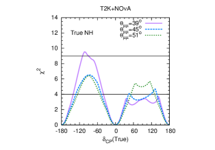
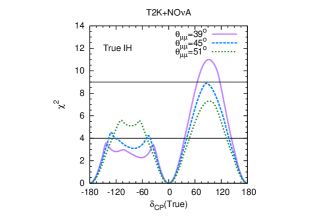
Figure 3.1: $\chi^{2}$ for CPV discovery vs true $\delta_{CP}$ for NO$\nu$A+T2K for $\sin^{2}2\theta_{13}=0.1$, three values of $\theta_{\mu\mu}$ and a true normal (left panel) or inverted (right panel) mass hierarchy.

The left panel gives the CP discovery for true NH, while the right panel depicts the results for true IH. From the figure, it may be observed that the CPV discovery of NO$\nu$A+T2K suffers a drop in one of the half-planes of $\delta_{CP}$ for all the three values of $\theta_{\mu\mu}$. The drop is in the region $[0^{\circ},180^{\circ}]$ (upper half-plane: UHP) if it is NH, and $[-180^{\circ},0^{\circ}]$ (lower half-plane: LHP) if it is IH. These are the unfavourable half-planes corresponding to the hierarchy-$\delta_{CP}$ degeneracy where the $\chi^{2}$ minima occurs with the wrong hierarchy. Here we can see that the results depend significantly on the true value of $\theta_{\mu\mu}$. As hierarchy sensitivity increases with $\theta_{\mu\mu}$, the CP sensitivity of the unfavourable half-planes increases with increasing $\theta_{\mu\mu}$. But on the other hand CP sensitivity decreases with increasing $\theta_{\mu\mu}$ in the favourable half-planes. We will discuss the reason for this in Section LABEL:dependence. There is also a drop around $\delta_{CP}=-90^{\circ}$ for true NH and $\theta_{23}=39^{\circ}$. This occurs because of the presence of octant-$\delta_{CP}$ degeneracy. As discussed earlier (see Fig. 2.9), the octant-$\delta_{CP}$ degeneracy occurs in LO-LHP for neutrinos and absent in antineutrinos. As in these plots we have considered T2K(8+0) and NO$\nu$A(3+3), the neutrino run dominates and thus the wrong octant solution appears at $\delta_{CP}=-90^{\circ}$ for true NH and $\theta_{23}=39^{\circ}$.

From these plots we observe that with the projected exposure of T2K and NO$\nu$A, $3\sigma$ CPV sensitivity can be achieved only around $\delta_{CP}=-90^{\circ}(+90^{\circ})$ if true hierarchy is NH (IH).

3.2.4 CP Sensitivity of Atmospheric Neutrinos

Now let us discuss the CP sensitivity of the atmospheric neutrino experiment ICAL.

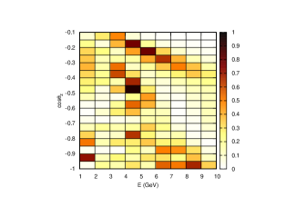
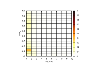
Figure 3.2: $S_{\mu}+S_{\overline{\mu}}$, a measure of ICAL $\delta_{CP}$-sensitivity in the $E-\cos{\theta_{z}}$ plane for $\sin^{2}2\theta_{13}=0.1$, $\sin^{2}\theta_{\mu\mu}=0.5$ and NH. The grid represents bins in energy and $\cos\theta_{z}$. The left panel is with ideal detector resolution and the right panel is with a resolution of $10^{\circ}$ in angle and $10\%$ in energy.

The muon events in atmospheric neutrinos get contributions from both $P_{\mu\mu}$ and $P_{e\mu}$. In these probabilities, the $\delta_{CP}$-dependent term always appears along with a factor of $\cos\Delta$ or $\sin\Delta$ (cf. Eq. 2.101). In atmospheric neutrinos, the baseline is associated with the direction of the incoming neutrinos or the zenith angle $\theta_{z}$. If we consider even a $10\%$ error range in the zenith angle and energy of the neutrino, the oscillating term varies over an entire cycle in this range. As a result, the $\delta_{CP}$-sensitivity of the channel gets washed out because of smearing. In Fig. 3.2, we have plotted the quantity $S=S_{\mu}+S_{\overline{\mu}}$ in the $E-\cos\theta_{z}$ plane, which is a measure of the $\delta_{CP}$-sensitivity of the atmospheric neutrino experiment. Here, $S_{\mu}=(\delta N_{\mu})^{2}/N_{\mu}(\textrm{avg})$, where $\delta N_{\mu}$ is the maximum difference in the number of events obtained by varying $\delta_{CP}$ and $N_{\mu}(\textrm{avg})$ is the average number of events over all values of $\delta_{CP}$ (and likewise $S_{\overline{\mu}}$ for $\overline{\mu}$ events). The quantity $S$ is thus a measure of the maximum possible relative variation in events due to $\delta_{CP}$ in each bin. In the left panel, we show the results for an ideal detector with an exposure of 500 kt yr, with infinite energy and angular precision. Here we see substantial sensitivity to $\delta_{CP}$, with $S$ exceeding $0.5$ in some bins [182]. However, when we introduce realistic resolutions ($10^{\circ}$ in angle and $10\%$ in energy), we see from the right panel of Fig. 3.2 that the sensitivity is lost. To study this point in more detail, we investigate how the intrinsic CP sensitivity of atmospheric neutrinos depend on the energy and angular resolutions and how much sensitivity can be achieved for an ideal detector. In Fig. 3.3 the CP violation discovery potential of ICAL is plotted as a function of the energy and angular resolution.

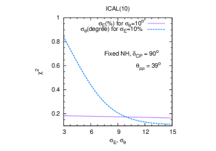
Figure 3.3: CP violation discovery potential of ICAL as a function of the detector energy and angular resolutions for $\delta_{CP}^{tr}=90^{\circ}$. $\theta_{\mu\mu}^{tr}=39^{\circ}$ and a true NH is assumed.

The curve for angular (energy) resolution is plotted by varying the respective smearing widths between $3^{\circ}-15^{\circ}$ ($3\%-15\%$) while holding the energy (angular) resolution fixed at $10\%(10^{\circ})$. The figure illustrates the significant role played by the angular resolution of an atmospheric neutrino detector in controlling the CP sensitivity. With present realistic values of detector smearing (15$\%$,15^∘), the CP sensitivity of such an experiment is washed out by averaging over bins in energy and direction, due to the coupling between $\delta_{CP}$ and $\Delta=\Delta_{31}L/4E$ in the term $\cos(\delta_{CP}+\Delta)$ in $P_{\mu e}$. With a hypothetical improved angular resolution of $3^{\circ}$, the CP violation discovery $\chi^{2}$ may reach values close to 1, going up to 5 for an ideal detector with no smearing.

Thus atmospheric neutrino experiments by themselves are not sensitive to $\delta_{CP}$. For beam experiments, since the direction of the neutrinos is known, angular smearing is not needed and hence the sensitivity to $\delta_{CP}$ is not compromised due to this reason.

3.2.5 Effect of ICAL on the CP Sensitivity of T2K and NO$\nu$A

In this section we discuss the combined CP sensitivity of the T2K, NO$\nu$A and ICAL detectors. Previously we have seen that CP sensitivity of T2K and NO$\nu$A is compromised due to unknown hierarchy and octant. An atmospheric neutrino detector like ICAL gives hierarchy and octant sensitivity which is remarkably stable over the entire range of $\delta_{CP}$, even though it does not offer any significant CPV discovery potential by itself. Thus the hierarchy and octant sensitivity of the atmospheric neutrinos can exclude the wrong solutions for CPV discovery.

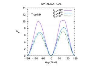
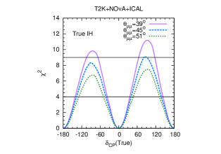
Figure 3.4: CPV discovery vs true $\delta_{CP}$ for NO$\nu$A+T2K+ICAL for $\sin^{2}2\theta_{13}=0.1$, three values of $\theta_{\mu\mu}$ and a true normal (left panel) or inverted (right panel) mass hierarchy.

In Fig. 3.4 we have plotted the combined CP sensitivity of NO$\nu$A+T2K+ICAL. Left panel is for true NH and right panel is for true IH. In these figures we see that when the information of ICAL is added to NO$\nu$A+T2K, the $\chi^{2}$ in the unfavourable region increases significantly. For NH and $\theta_{23}=39^{\circ}$, the shape of the curve shows that the sensitivity of ICAL is not sufficient to rule out the wrong hierarchy minima completely for $\delta_{CP}=90^{\circ}$. We also observe that after the addition of ICAL data, the $\theta_{\mu\mu}$ dependence in the unfavourable region becomes similar to that of favourable region. The wrong octant solution for NH, $\theta_{23}=39^{\circ}$ and $\delta_{CP}=-90^{\circ}$ also vanishes. The advantage offered by combining ICAL with the LBL data is most prominent for $\theta_{23}=39^{\circ}$ and progressively diminishes with increasing $\theta_{23}$. In general, the atmospheric neutrino contribution to the CPV discovery potential of NO$\nu$A+T2K+ICAL is effective till the wrong solutions are disfavoured and the minimum comes with the true hierarchy and octant. Once that is achieved, a further increase in the sensitivity of atmospheric neutrinos will not affect the CPV discovery results, since atmospheric neutrinos by themselves do not have CPV sensitivity for realistic resolutions. From the figures we can see that for true NH (IH), T2K+NO$\nu$A can discover CPV at $2\sigma$ for $\sim$ 28%(29%) fraction of $\delta_{CP}$ values for $\theta_{\mu\mu}=39^{\circ}$. By adding ICAL information, this improves to $\sim$ 58%. For maximal CPV ($\delta_{CP}=\pm 90^{\circ}$), inclusion of ICAL gives a $\sim 3\sigma$ signal for both hierarchies. Without the ICAL contribution this is true only in one of the half-planes depending on the hierarchy.

To study the effect of ICAL detector resolutions on the results, we plot in Fig. 3.5 the CPV discovery potential of NO$\nu$A+T2K+ICAL for $\theta_{\mu\mu}=39^{\circ}$ and true NH assuming two sets of energy and angular smearing for ICAL – (15%,$15^{\circ}$) and (10%,$10^{\circ}$).

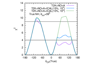
Figure 3.5: CPV discovery vs true $\delta_{CP}$ for NO$\nu$A+T2K and NO$\nu$A+T2K+ICAL (500 kt yr) for two sets of ICAL detector resolutions for $\theta_{\mu\mu}=39^{\circ}$, $\sin^{2}2\theta_{13}=0.1$ and true NH.

In the former case, an indication of CPV at $2\sigma$ is seen to be achieved around $\delta_{CP}=+90^{\circ}$ but the improvement in the CP sensitivity is very less. For the latter (better) smearing set, though the $\chi^{2}$ minimum still comes with the wrong hierarchy but the sensitivity increases significantly in the unfavourable half-plane. An improvement in the resolution beyond (10%,$10^{\circ}$) can improve the CP sensitivity even more by excluding the wrong hierarchy solution completely. For $\delta_{CP}=-90^{\circ}$, the drop due to the wrong octant solution is no longer visible after adding the ICAL data with (15%,$15^{\circ}$) resolution. Since the wrong solution is already removed, there is no further improvement in the CP sensitivity for this value of $\delta_{CP}$ when the ICAL resolution improved to (10%,$10^{\circ}$).

In order to gauge the contribution from ICAL with a reduced exposure, we plot in Fig. 3.6 the CPV discovery as a function of $\delta_{CP}$ for NO$\nu$A+T2K and NO$\nu$A+T2K+ICAL for two ICAL exposures, 250 kt yr and 500 kt yr for $\theta_{\mu\mu}=39^{\circ}$, $\sin^{2}2\theta_{13}=0.1$ and true NH, using the (10%,$10^{\circ}$) ICAL resolution set.

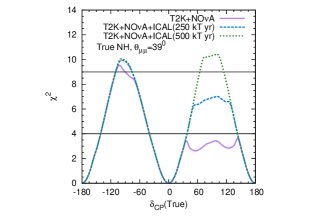
Figure 3.6: CPV discovery vs true $\delta_{CP}$ for NO$\nu$A+T2K and NO$\nu$A+T2K+ICAL for two exposures, 250 kt yr and 500 kt yr for $\theta_{\mu\mu}=39^{\circ}$, $\sin^{2}2\theta_{13}=0.1$ and true NH. The ICAL resolutions are assumed to be 10$\%$ in energy and 10^∘ in angle.

The figure shows that with an ICAL exposure of 250 kt yr, a 2.6$\sigma$ hint for CPV is achieved for $\delta_{CP}=+90^{\circ}$.

3.2.6 A Chronological Study of $\delta_{CP}$ Using T2K, NO$\nu$A and ICAL

In this section we further explore the CPV discovery potential of T2K and NO$\nu$A using different run times. We also use exposure beyond that projected in order to assess the capabilities of these experiments with enhanced statistics. In addition to CPV discovery, we will present the results for $\delta_{CP}$ precision in $\delta_{CP}$ (true) vs $\delta_{CP}$ (test) plane. We will also study the effect of ICAL in improving the CP sensitivity of T2K and NO$\nu$A. For our study we will consider the following exposures of T2K, NO$\nu$A and ICAL:

• 5 year run of T2K: either (5+0) configuration or (3+2) configuration and 10 year run of T2K in (5+5) configuration.

• For NO$\nu$A we will take either (3+3) or (5+5) configuration.

• For ICAL we will consider either 5 year (250 kt yr) or 10 year (500 kt yr) exposure.

For detail see [183].

In Table 3.1 we summarize the maximum values of CP violation discovery potential, and the percentage of true $\delta_{CP}$ values capable of giving a CP violation discovery signal at 2$\sigma$ and 3$\sigma$, for different combinations of the experiments T2K, NO$\nu$A and ICAL.

Experiment (exposure)	max $\chi^{2}$ in		$\delta_{CP}$ fraction for CPV
	UVHP	FVHP	$2\sigma$	$3\sigma$
T2K(8+0)+NO$\nu$A(3+3)	$3.5$	$9.5$	$28\%$	$5\%$
T2K(8+0)+NO$\nu$A(3+3)+ICAL	$10.5$	$10.0$	$58\%$	$24\%$
T2K(3+2)	$0.9$	$3.3$	$-$	$-$
T2K(5+0)	$1.2$	0.8	$-$	$-$
T2K(3+2) + NO$\nu$A(3+3)	$3.1$	7.5	$24\%$	$-$
T2K(5+0) + NO$\nu$A(3+3)	$3.3$	8.2	$25\%$	$-$
T2K(5+0) + NO$\nu$A(5+5)	$4.8$	10.7	$36\%$	$11\%$
T2K(5+5) + NO$\nu$A(5+5)	$4.9$	12.5	$41\%$	$17\%$
T2K(5+0) + NO$\nu$A(3+3) + ICAL 5	$6.4$	8.3	$52\%$	$-$
T2K(5+0) + NO$\nu$A(5+5) + ICAL 5	$7.4$	10.8	$60\%$	$12\%$
T2K(5+5) + NO$\nu$A(5+5) + ICAL 5	$7.7$	12.7	$62\%$	$17\%$
T2K(5+0) + NO$\nu$A(5+5) + ICAL 10	$10.7$	11.0	$60\%$	$27\%$
T2K(5+5) + NO$\nu$A(5+5) + ICAL 10	$11.1$	12.7	$62\%$	$36\%$

Table 3.1: Values of maximal CP violation discovery $\chi^{2}$ in the favourable and unfavourable half-planes (FVHP and UVHP) and percentage of true $\delta_{CP}$ values allowing CP violation discovery at 2$\sigma$/3$\sigma$ for combinations of experiments. Here $\theta_{\mu\mu}^{tr}=39^{\circ}$, $\sin^{2}2\theta_{13}=0.1$ and true NH.

From the table we see that, with the projected exposure, the combination of T2K and NO$\nu$A gives $2\sigma$ CPV discovery sensitivity for $28\%$ fraction of total $\delta_{CP}$ values and $3\sigma$ CPV discovery sensitivity for $5\%$ fraction of total $\delta_{CP}$ values. With the inclusion of ICAL, the sensitivity improves to $58\%$ and $24\%$ for $2\sigma$ and $3\sigma$ respectively. If one considers the most optimistic run times for these experiments i.e., the T2K(5+5) and NO$\nu$A(5+5) configurations, then also with the inclusion of 10 year data of ICAL gives a maximum CPV discovery sensitivity corresponding to a fraction of $62\%$ for $2\sigma$ and $36\%$ for $3\sigma$ of the total $\delta_{CP}$ values.

From these results we understand that, to establish CPV (as well as CP precision) at higher confidence level, covering larger fraction of $\delta_{CP}$ values, one needs experiments more powerful than T2K and NO$\nu$A. This is also true for determining hierarchy and octant. In [154, 147] it has been shown that the combination of T2K and NO$\nu$A is not sensitive enough to determine hierarchy and octant with a very high confidence level. To achieve higher sensitivity, several experiments have been proposed which will have comparatively longer baselines and powerful neutrino beams. The projects LBNO and LBNE are the examples of such proposed long-baseline experiments. LBNO is an European project where neutrinos will be delivered from the CERN accelerator, whereas for the LBNE project, Fermilab will generate the neutrinos. As the exact design of these experiments are still under consideration, one needs to carry out a detail analysis to find out the optimal configuration for measuring the oscillation parameter with greater confidence level. In the next two sections we will study the physics potential of the LBNO and LBNE experiments and find out their optimal exposure to determine the unknown neutrino oscillation parameters.

3.3 Physics Potential of LBNO in Conjunction with T2K, NO$\nu$A and ICAL

In this section, we will discuss the contributions of NO$\nu$A, T2K, ICAL@INO and LBNO towards determining the mass hierarchy, octant of $\theta_{23}$ as well as for discovery of CP violation. As the precise configuration of LBNO is under consideration, our aim is to determine the configuration for LBNO with ‘adequate’ exposure in conjunction with T2K, NO$\nu$A and ICAL, which can determine the unknown oscillation parameters. The ‘adequate’ configuration is defined as one with the minimal exposure which would give a 5$\sigma$ discovery potential for hierarchy and octant and 3$\sigma$ discovery potential for $\delta_{CP}$ in the most unfavourable case. This configuration can be viewed as the first step in a staged approach that has been advocated by previous studies [184].

The plan of this section is as follows. First we give the experimental specifications that we have used for the proposed LBNO experiment and other simulation details. The next three subsections thereafter are devoted to the analysis of the experimental reach of the combination of experiments for determining the mass hierarchy, octant of $\theta_{23}$ and discovery of CP violation respectively.

3.3.1 Experimental Specifications and Other Simulation Details

Out of the various possible options for the LBNO experiment as described in chapter 2 , we consider the following three options that are prominent in the literature: CERN-Pyhäsalmi, CERN-Slanic and CERN-Fréjus. The specifications that we have used in this study are listed below in Table 3.2. We have used the superbeam fluxes from Ref. [185].

For NO$\nu$A, T2K and ICAL we consider the same specification as mentioned in section 3.2. For NO$\nu$A we have considered an equal 3 year running in both neutrino and antineutrino mode. For T2K we assumed a total exposure corresponding to $8\times 10^{21}$ POT running in completely neutrino mode and we have taken 10 year running of ICAL, which corresponds to a total exposure of 500 kt-yr.

Detector site	Pyhäsalmi	Slanic	Fréjus
Baseline	$2290$ km	$1540$ km	$130$ km
Detector Type	LArTPC	LArTPC	Water Čerenkov
Proton energy	$50$ GeV	$50$ GeV	$4.5$ GeV
Resolutions, efficiencies	as in Ref. [184]	as in Ref. [184]	as in Ref. [186]
Signal systematics	5%	5%	5%
Background systematics	5%	5%	10%

Table 3.2: Experimental characteristics of the LBNO options.

We have fixed the ‘true’ values of the parameters close to the values obtained from global fits of world neutrino data. We have taken: $\sin^{2}\theta_{12}=0.304$, $|\Delta_{31}|=2.4\times 10^{-3}$ eV², $\Delta_{21}=7.65\times 10^{-5}$ eV² and $\sin^{2}2\theta_{13}=0.1$. Three representative true values of $\theta_{23}$ have been considered – $39^{\circ}$, $45^{\circ}$ and $51^{\circ}$ (except in the case of octant determination where a wider range and more intermediate values have been included). The true value of $\delta_{CP}$ is varied in its entire allowed range. All our results are shown for both NH and IH. The ‘test’ values of the parameters are allowed to vary in the following ranges – $\theta_{23}\in\left[35^{\circ},55^{\circ}\right]$, $\sin^{2}2\theta_{13}\in\left[0.085,0.115\right]$, $\delta_{CP}\in\left[0,360^{\circ}\right)$. The test hierarchy is also allowed to run over both possibilities. We have imposed a prior on the value of $\sin^{2}2\theta_{13}$ with an error $\sigma(\sin^{2}2\theta_{13})=0.005$. We have however not imposed any prior on the atmospheric parameters, instead allowing the $\nu_{\mu}$ disappearance channels to restrict their range. In all our simulations, we have taken into account the three-flavour-corrected definitions of the atmospheric parameters [180, 179, 181] as given in Eqs. 3.5 and 3.6.

The aim of this exercise is to determine the least exposure required from LBNO in order to determine hierarchy and octant with a statistical significance corresponding to $\chi^{2}=25$ and that CP violation detected with $\chi^{2}=9$ for 20% value of $\delta_{CP}$. Therefore, we have plotted the sensitivity to hierarchy/octant/CP violation for various different exposures of LBNO, combined with NO$\nu$A, T2K and INO. From this, we estimate the adequate amount of exposure required by LBNO. We express the exposure in units of POT-kt. This is a product of three experimental quantities:

$$\textrm{exposure (POT-kt)}=\textrm{beam intensity (POT/yr)}\times\textrm{runtime (yr)}\times\textrm{detector mass (kt)}~{}.$$ (3.7)

Thus, a given value of exposure can be achieved experimentally by adjusting the intensity, runtime and detector mass. The advantage of using this measure is that while the physics goals are expressed in terms of simply one number (the exposure), the experimental implementation of this exposure can be attained by various combinations of beam, detector and runtime settings. For example, an exposure of $45\times 10^{21}$ POT-kt could be achieved with a $1.5\times 10^{21}$ POT/yr beam running for $3$ years with a $10$ kt detector or a $3\times 10^{21}$ POT/yr beam running for $3$ years with a $5$ kt detector. According to our terminology, the exposures given correspond to each mode (neutrino and antineutrino). Thus, a runtime of $n$ years implies $n$ years each in neutrino and antineutrino mode totaling to $2n$ years.

3.3.2 Determination of Mass Hierarchy

Among the three chosen prospective baselines for LBNO, the 130 km set-up has the lowest hierarchy sensitivity due to small matter effects. As the baseline increases, the hierarchy sensitivity becomes better because of enhanced matter effects. In particular, the 2290 km set-up has the unique advantage of being close to satisfying the bimagic conditions [151, 153, 152](cf. Section 2.4.1). This feature makes the baseline particularly suited for hierarchy determination. The above features are reflected in Fig. 3.7.

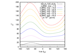
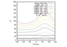
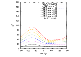
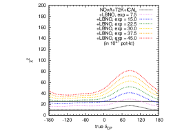
Figure 3.7: Hierarchy sensitivity $\chi^{2}$ vs true $\delta_{CP}$. The top (bottom) panels are for the $2290$ ($1540$) km baseline. The left (right) panels are for true NH (IH). In all the panels, the lowermost densely-dotted (black) curve is for NO$\nu$A+T2K+ICAL, while the curves above are for NO$\nu$A+T2K+ICAL+LBNO, for various values of LBNO exposure. All the plotted sensitivities are for the least favourable value of true $\theta_{23}$.

In each of the panels of Fig. 3.7, the lowermost densely-dotted (black) curve shows the hierarchy sensitivity of the combination NO$\nu$A+T2K+ICAL. We see that these experiments can collectively give $\chi^{2}\approx 9$ sensitivity to the hierarchy. Therefore, in keeping with our aims, we need to determine the minimum exposure for LBNO, such that the combination NO$\nu$A+T2K+ICAL+LBNO crosses the threshold of $\chi^{2}=25$ for all values of $\delta_{CP}$. For this, we have plotted the combined sensitivity of NO$\nu$A+T2K+ICAL+LBNO for various values of LBNO exposure (in units of $10^{21}$ POT-kt). The results are shown for two baselines – $2290$ km and $1540$ km, and for both hierarchies. We find that our results are consistent with those shown in Ref. [92], for the same beam power and oscillation parameters. For the baseline of $130$ km, it is not possible to cross $\chi^{2}=25$ even with extremely high exposure. Therefore we have not shown the corresponding plots for this baseline. We considered three true values of $\theta_{23}$ – $39^{\circ},45^{\circ},51^{\circ}$ and chose the $\chi^{2}$ corresponding to the least favourable of these in generating the figures. Thus, our results represent the most conservative case. We find that in most cases, the minimum $\chi^{2}$ for hierarchy determination occurs for true $\theta_{23}=39^{\circ}$.

Finally, in Fig. 3.8, we have condensed all this information into a single plot.

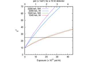
Figure 3.8: Hierarchy sensitivity $\chi^{2}$ vs LBNO exposure, for both baselines and hierarchies under consideration. The value of exposure shown here is adequate to exclude the wrong hierarchy for all values of $\delta_{CP}$. The additional axis along the upper edge of the graph shows the required total POT assuming a detector mass of $10$ kt.

We have shown the sensitivity for the experiments as a function of the LBNO exposure. We see that for $2290$ ($1540$) km, it is sufficient for LBNO to have an exposure of around $7\times 10^{21}$ ($21\times 10^{21}$) POT-kt in order to get a $\chi^{2}=25$ for all values of $\delta_{CP}$. Along the upper edge of the graph, we have provided an additional axis, which denotes the total POT required if we assume that the detector has a mass of $10$ kt. For $2290$ ($1540$) km, we need a total of $0.7\times 10^{21}$ ($2.1\times 10^{21}$) POT. To get some idea of the time scale involved we consider for instance the beam intensity used in Ref. [184] which corresponds to $3\times 10^{21}$ POT/yr delivered by a $50$ GeV proton beam from CERN with beam power $1.6$ MW. The total POT of $0.7\times 10^{21}$ for a 10 kt detector at the $2290$ ($1540$) km baseline would thus need less than $1$ ($2$) years (total, inclusive of $\nu$ and $\overline{\nu}$ runs) to establish mass hierarchy with $\chi^{2}=25$.

Fig. 3.9, demonstrates the synergy between long-baseline and atmospheric neutrino experiments.

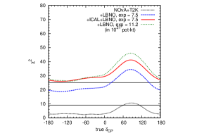
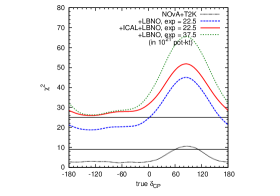
Figure 3.9: Hierarchy sensitivity $\chi^{2}$ for different combinations of experiments, demonstrating the synergy between them. The left (right) panel is for a LBNO baseline of $2290$ ($1540$) km, assuming IH to be true. With only T2K+NO$\nu$A+LBNO (dashed, blue), the sensitivity is lower than for T2K+NO$\nu$A+LBNO+ICAL (red, solid). Without ICAL data, the LBNO exposure would have to be increased substantially (dotted, green) in order to get comparable sensitivity. All the plotted sensitivities are for the least favourable value of true $\theta_{23}$.

We have chosen the $2290$ ($1540$) km baseline as an illustrative case in the left (right) panels, with the true hierarchy assumed to be IH. The densely-dotted (black) curve at the bottom shows the hierarchy sensitivity of NO$\nu$A+T2K without any atmospheric neutrino data included in the analysis. If the atmospheric information is not included then the combination of NO$\nu$A+T2K+LBNO would need about $11\times 10^{21}$ POT-kt in order to attain $\chi^{2}=25$, for the 2290 baseline. Assuming a beam intensity of $3\times 10^{21}$ POT/yr this would require less than a year to measure the hierarchy with a 10 kt detector. Combining these with ICAL reduces the exposure to $7\times 10^{21}$ POT-kt. Thus, for the same beam intensity one can achieve the same sensitivity with a 7 kt detector. Similar conclusions can be drawn for the 1540 km set-up. It should be noted that the numbers in Fig. 3.9 are sample values at which the simulations are performed. The exposure required for each set-up to attain the ‘adequate’ values can be read off from Fig.  3.8 and is presented in Table 3.3.

Adequate exposure for	$2290$ km	$1540$ km	$130$ km
Hierarchy exclusion at	$7(11)\times 10^{21}$	$21(37)\times 10^{21}$	$-$
$\chi^{2}=25$
Octant exclusion for $39^{\circ}$	$83(113)\times 10^{21}$	$83(113)\times 10^{21}$	$400(600)\times 10^{21}$
at $\chi^{2}=25$
CP violation detection
at $\chi^{2}=9$	$240(240)\times 10^{21}$	$170(170)\times 10^{21}$	$35(100)\times 10^{21}$
for 20% fraction of $\delta_{CP}$

Table 3.3: Summary of results: ‘adequate’ exposure in POT-kt for three LBNO configurations in conjunction with T2K,NO$\nu$A and ICAL to achieve the physics goals. The numbers given in parentheses indicate the required exposure if atmospheric neutrino data from ICAL is not included.

3.3.3 Determination of Octant of $\theta_{23}$

The octant sensitivity of long-baseline experiments has been studied in detail recently in [147, 191] and also in conjunction with atmospheric neutrino experiments [169]. As in the case of hierarchy, adding information from various experiments enhances the sensitivity. However, the precise knowledge of the value of $\theta_{13}$ also plays a very crucial role in enhancing the octant sensitivity [130]. In Fig. 3.10, the lowermost densely-dotted (black) curve denotes the ability of NO$\nu$A+T2K+ICAL to determine the octant as a function of the true value of $\theta_{23}$ in nature.

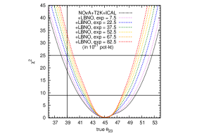
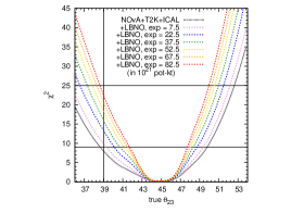
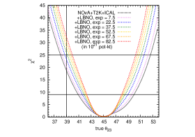
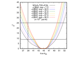
Figure 3.10: Octant sensitivity $\chi^{2}$ vs true $\theta_{23}$. The top (bottom) panels are for the $2290$ ($1540$) km baseline. The left (right) panels are for true NH (IH). In all the panels, the lowermost densely-dotted (black) curve is for NO$\nu$A+T2K+ICAL, while the curves above are for NO$\nu$A+T2K+ICAL+LBNO, for various values of LBNO exposure. All the plotted sensitivities are for the least favourable value of true $\delta_{CP}$.

Again, the other curves denote the combined sensitivity of NO$\nu$A+T2K+ICAL+LBNO(2290 km and 1540 km) for various values of LBNO exposure (in units of $10^{21}$ POT-kt). We generated the results for various true values of $\delta_{CP}$, and the results shown in the figure are for the most conservative case. We see that only with NO$\nu$A+T2K+ICAL, the octant can be determined at $>3\sigma$ C.L. when $\theta_{23}=39^{\circ}$. For values closer to $45^{\circ}$, the sensitivity gets steadily worse. The addition of LBNO data increases the sensitivity. For the range of exposures considered, it is possible to get a $\chi^{2}=25$ sensitivity to the octant as long as $\theta_{23}$ deviates from maximality by at least $\sim 6^{\circ}$.

In Fig. 3.11, we have shown how the octant sensitivity of these experiments increases as the exposure for LBNO is increased.

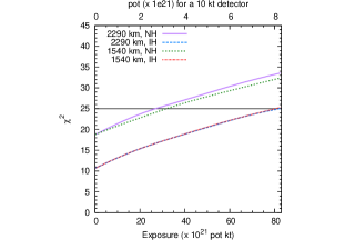
Figure 3.11: Octant sensitivity $\chi^{2}$ vs LBNO exposure, for the $2290$ km and $1540$ km baselines and both hierarchies, with $\theta_{23}=39^{\circ}$. The additional axis along the upper edge of the graph shows the required total POT assuming a detector mass of $10$ kt.

For this, we have chosen the true value of $\theta_{23}$ to be $39^{\circ}$. Because of the better performance of NO$\nu$A+T2K+ICAL when NH is true, the adequate exposure for LBNO is higher when IH is true. Given our current state of ignorance about the true hierarchy in nature, we give the $\chi^{2}$ for the worst case i.e.,we present the octant sensitivity results (cf. Table 3.3) for the hierarchy that requires a higher exposure. The fig shows that it is sufficient to have an exposure of around $83\times 10^{21}$ POT-kt to reach $\chi^{2}=25$ for both the baselines. The upper axis shows the total POT required, with a $10$ kt detector. For instance, we see that $8.3\times 10^{21}$ POT is sufficient if we have a $10$ kt detector. This translates to a runtime of a little under $3$ years in each $\nu$ and $\overline{\nu}$ mode, given an intensity of $3\times 10^{21}$ POT/yr.

Fig. 3.12 is the same as Fig. 3.10, but for the $130$ km baseline.

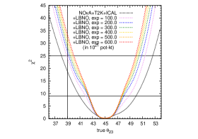
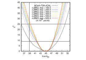
Figure 3.12: Octant sensitivity $\chi^{2}$ vs true $\theta_{23}$ for the $130$ km baseline. The left (right) panel is for true NH (IH). In both panels, the lowermost densely-dotted (black) curve is for NO$\nu$A+T2K+ICAL, while the curves above are for NO$\nu$A+T2K+ICAL+LBNO, for various values of LBNO exposure. All the plotted sensitivities are for the least favourable value of true $\delta_{CP}$.

As expected, because of smaller matter effects, the exposure required to determine the octant is much higher than that for the other two baselines. However, for a large mass detector like MEMPHYS that is being planned for the Fréjus site, this exposure is not difficult to attain. The sensitivity as a function of LBNO exposure for this baseline is shown in Fig. 3.13.

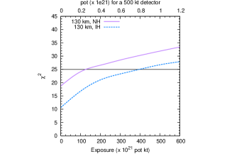
Figure 3.13: Octant sensitivity $\chi^{2}$ vs LBNO exposure, for the $130$ km baseline and both hierarchies, with $\theta_{23}=39^{\circ}$. The additional axis along the upper edge of the graph shows the required total POT assuming a detector mass of $500$ kt.

We need an exposure of around $400\times 10^{21}$ POT-kt in this case. For this graph, the upper axis shows the required POT if we consider a $500$ kt detector, as proposed for MEMPHYS [186]. We see that for such a large mass detector, only around $0.8\times 10^{21}$ POT is adequate to exclude the octant for $\theta_{23}=39^{\circ}$.

Fig. 3.14 shows the synergy between LBL experiments and ICAL.

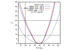
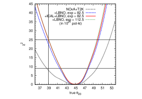
Figure 3.14: Octant sensitivity $\chi^{2}$ for different combinations of experiments, demonstrating the synergy between them. The left (right) panel is for a LBNO baseline of $2290$ ($1540$) km, assuming IH to be true. With only T2K+NO$\nu$A+LBNO (dashed, blue), the sensitivity is lower than for T2K+NO$\nu$A+LBNO+ICAL (red, solid). Without ICAL data, the LBNO exposure would have to be increased substantially (dotted, green) in order to get comparable sensitivity. All the plotted sensitivities are for the least favourable value of true $\delta_{CP}$.

In the left (right) panel, we have chosen the LBNO baseline of $2290$ ($1540$) km to illustrate this point. IH is assumed to be the true hierarchy. The sensitivity of T2K+NO$\nu$A alone (densely-dotted, black curve) is enhanced by adding data from ICAL and LBNO. The solid (red) curve in the left panel shows that an exposure of $82.5\times 10^{21}$ POT-kt is enough to determine the octant with $\chi^{2}=25$ at $39^{\circ}$. But without ICAL data (dashed, blue curve), the sensitivity would be lower. The dotted (green) curve shows that only with $112.5\times 10^{21}$ POT-kt (more than 35% higher than the adequate amount), can we attain $\chi^{2}=25$ without ICAL. For $1540$ km (right panel) also, similar features are observed. This demonstrates the advantage of adding atmospheric neutrino data.

3.3.4 Evidence for CP Violation

Now, we discuss the detection of CP violation. We show our results as a function of true $\delta_{CP}$ in Fig. 3.15.

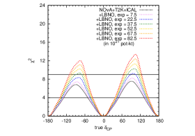
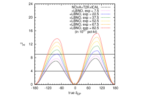
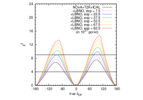
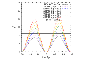
Figure 3.15: CP violation detection $\chi^{2}$ vs true $\delta_{CP}$. The top (bottom) panels are for the $2290$ ($1540$) km baseline. The left (right) panels are for true NH (IH). In all the panels, the lowermost densely-dotted (black) curve is for NO$\nu$A+T2K+ICAL, while the curves above are for NO$\nu$A+T2K+ICAL+LBNO, for various values of LBNO exposure. All the plotted sensitivities are for the least favourable value of true $\theta_{23}$.

As in the case of hierarchy exclusion, we have minimised over three different true values of $\theta_{23}$ and have chosen the most conservative case among these for each true $\delta_{CP}$.

We see in Fig. 3.15 that with NO$\nu$A+T2K+ICAL, only around $\chi^{2}=4$ can be attained, for a small range of $\delta_{CP}$ values around $\pm 90^{\circ}$. Adding LBNO (2290 km and 1540 km) data with increasing exposure can enhance this and can even help to achieve $\chi^{2}=9$ for CP detection for some range of $\delta_{CP}$. In Fig. 3.16, we have plotted the fraction of $\delta_{CP}$ for which CP violation can be detected with $\chi^{2}=9$, as a function of the LBNO exposure.

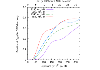
Figure 3.16: Fraction of the full $\delta_{CP}$ range for which it is possible to detect CP violation (exclude $\delta_{CP}=0,180^{\circ}$) at $3\sigma$ vs LBNO exposure, for the $2290$ km and $1540$ km baselines and both hierarchies. The additional axis along the upper edge of the graph shows the required total POT assuming a detector mass of $10$ kt.

As an example, if we aim to detect CP violation for at least 20% of $\delta_{CP}$ values, then we require around $240\times 10^{21}$ ($170\times 10^{21}$) POT-kt exposure from LBNO with a baseline of $2290$ ($1540$) km. It can also be seen from the figure that with $350\times 10^{21}$ POT-kt exposure, the maximum CP fraction for which a $3\sigma$ sensitivity is achievable ranges from 30% to 40%. The upper axis shows that these values correspond to $24\times 10^{21}$ ($17\times 10^{21}$) POT, if we consider a $10$ kt detector.

Figs. 3.17 and 3.18 show the results for the $130$ km option.

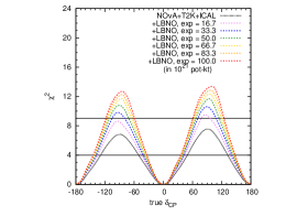
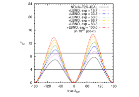
Figure 3.17: CP violation detection $\chi^{2}$ vs true $\delta_{CP}$ for the $130$ km baseline. The left (right) panel is for true NH (IH). In both panels, the lowermost densely-dotted (black) curve is for NO$\nu$A+T2K+ICAL, while the curves above are for NO$\nu$A+T2K+ICAL+LBNO, for various values of LBNO exposure. All the plotted sensitivities are for the least favourable value of true $\theta_{23}$.

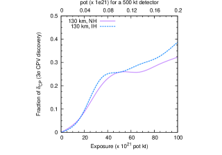
Figure 3.18: Fraction of the full $\delta_{CP}$ range for which it is possible to detect CP violation at $3\sigma$ vs LBNO exposure, for the $130$ km baseline and both hierarchies. The additional axis along the upper edge of the graph shows the required total POT assuming a detector mass of $500$ kt.

Once again, we see that an exposure much higher than the longer baselines is required. In this case, CP detection for 20% $\delta_{CP}$ values requires an exposure of around $35\times 10^{21}$ POT-kt. This is not difficult to achieve with a large MEMPHYS-like detector. In fact, the total POT required by a $500$ kt detector at $130$ km is only around $0.07\times 10^{21}$ POT. Moreover, an underground megaton scale detector like MEMPHYS can also be used to collect atmospheric neutrino data [192], which can further enhance the sensitivity because of the ability of the atmospheric neutrinos to rule out the wrong hierarchy solutions.

In Fig. 3.19, we have demonstrated the synergy between atmospheric and long-baseline experiments for the baseline of $130$ km and with NH.

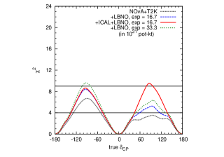
Figure 3.19: CP detection sensitivity $\chi^{2}$ for different combinations of experiments, demonstrating the synergy between them. This plot is for a LBNO baseline of $130$ km, assuming NH to be true. With only T2K+NO$\nu$A+LBNO (dashed, blue), the sensitivity is lower than for T2K+NO$\nu$A+LBNO+ICAL (red, solid). Without ICAL data, the LBNO exposure would have to be increased substantially (dotted, green) in order to get comparable sensitivity. All the plotted sensitivities are for the least favourable value of true $\theta_{23}$.

We see that with only T2K+NO$\nu$A (densely-dotted, black curve), one suffers from the hierarchy-$\delta_{CP}$ degeneracy in the unfavourable region of $\delta_{CP}$. This degeneracy is lifted by adding information from other experiments. On adding data from ICAL and $16.7\times 10^{21}$ POT-kt of LBNO (solid, red curve), we just reach $\chi^{2}=9$ sensitivity. With the same LBNO exposure, absence of ICAL data reduces the detection reach, as seen from the dashed (blue) curve. Reaching $\chi^{2}=9$ without ICAL will require the LBNO exposure to be doubled, as the dotted (green) curve shows. Thus ICAL plays a significant role in $\delta_{CP}$ measurement for this baseline. For the two longer baselines, LBNO even with very low exposure in conjunction with T2K and NO$\nu$A can break the hierarchy-$\delta_{CP}$ degeneracy by excluding the wrong hierarchy solution. Therefore, the contribution of ICAL towards detecting CP violation becomes redundant in this case.

3.4 Physics Potential of LBNE in Conjunction with T2K, NO$\nu$A and ICAL

In this section, we explore the sensitivity reach of the LBNE experiment in determining the remaining unknowns in neutrino oscillation, in combination with the other experiments T2K, NO$\nu$A and ICAL. In our study we carry out a similar analysis as that of LBNO i.e., we determine the most conservative specifications that this experiment needs, in order to measure the remaining unknown parameters to a specified level of precision. Addition to that, we will also study the effect of near detector in constraining systematic error, the role of second oscillation maxima. We will also present an optimisation study of neutrino and antineutrino run of LBNE.

3.4.1 Experimental Specifications and Other Simulation Details

As mentioned in chapter 3.3 for LBNE, there are two options being considered for the proton beam - 80 GeV and 120 GeV. In our study, we have chosen the 120 GeV proton beam. As the neutrino flux decreases with proton energy, this gives us a lower flux of neutrinos and hence a conservative estimate of our results.

The specifications for the liquid argon detector have been taken from Ref. [91]. In this study we use the flux corresponding to 1.2 MW beam power [193]. However we give our results in terms of MW-kt-yr. This will enable one to interpret the results in terms of varying detector volume, timescale and beam power. Note that although we use the flux corresponding to 1.2 MW beam power, if the accelerator geometry remains the same, then the change in the value of the beam power will proportionally change the flux. Therefore, the flux for a different value of beam power can be obtained by simply scaling the ‘standard’ flux file by the appropriate factor.

The specifications for T2K, NO$\nu$A and ICAL is same as that of LBNO analysis.

In the analyses that follow, we have evaluated the $\chi^{2}$ for determining the mass hierarchy, octant of $\theta_{23}$ and CP violation using a combination of LBNE and the current/upcoming experiments T2K, NO$\nu$A and ICAL. For each set of ‘true’ values assumed, we evaluate the $\chi^{2}$ marginalised over the ‘test’ parameters. For true $\theta_{23}$, we have considered three values – $39^{\circ}$, $45^{\circ}$ and $51^{\circ}$ which are within the current $3\sigma$ allowed range. The systematic uncertainties are parametrised in terms of four nuisance parameters – signal normalisation error (2.5%), signal tilt error (2.5%), background normalisation error (10%) and background tilt error (2.5%).

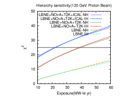
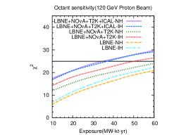
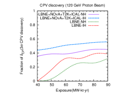
Figure 3.20: Hierarchy (Octant) sensitivity $\chi^{2}$ vs LBNE exposure, for both hierarchies in the left (middle) panel. The value of exposure shown here is adequate to exclude the wrong hierarchy for all values of $\delta_{CP}$. Two additional sets of curves are shown to show the fall in $\chi^{2}$ without data from ICAL, and the hierarchy sensitivity of LBNE alone. The right panel shows the fraction of $\delta_{CP}$ range for which it is possible to exclude the CP conserving cases of $0$ and $180^{\circ}$, at the $\chi^{2}=9$ level. An additional set of curves is shown to show the the CP sensitivity of LBNE alone.

To economise the configuration of LBNE with the help of the current generation of experiments, We evaluate the ‘adequate’ exposure for LBNE. The qualifier ‘adequate’, as defined in the context of LBNO, means the exposure required from the experiment to determine the hierarchy and octant with $\chi^{2}=25$, and to detect CP violation with $\chi^{2}=9$. To do so, we have varied the exposure of LBNE, and determined the combined sensitivity of LBNE along with T2K, NO$\nu$A and ICAL. The variation of total sensitivity with LBNE exposure tells us what the adequate exposure should be. In this study, we have quantified the exposure for LBNE in units of MW-kt-yr. This is a product of the beam power (in MW), the runtime of the experiment (in years) and the detector mass (in kilotons). As a phenomenological study, we will only specify the total exposure. This may be interpreted experimentally as different combinations of beam power, runtime and detector mass whose product quantifies the exposure. For example, an exposure of 20 MW-kt-yr could be achieved by using a 10 kt detector for 2 years (in each, $\nu$ and $\overline{\nu}$ mode), with a 1 MW beam. We use events in the energy range 0.5 - 8 GeV for LBNE which covers both first and second oscillation maxima.

3.4.2 Adequate Exposure for LBNE

3.4.2.1 Hierarchy Sensitivity

In the left panel of Fig. 3.20, we have shown the combined sensitivity of LBNE, NO$\nu$A, T2K and ICAL for determining the mass hierarchy, as the exposure for LBNE is varied. Note that the hierarchy sensitivity depends very strongly on the true value of $\delta_{CP}$ and $\theta_{23}$. In this study, as in LBNO, we are interested in finding out the least exposure needed for LBNE, irrespective of the true values of the parameters in nature. Therefore, we have evaluated the $\chi^{2}$ for various true values of these parameters, and taken the most conservative case out of them. Thus, the exposure plotted here is for the most unfavourable values of true $\delta_{CP}$ and $\theta_{23}$. Since hierarchy sensitivity of the $P_{\mu e}$ channel increases with $\theta_{23}$, the worst case is usually found at the lowest value considered which is $\theta_{23}=39^{\circ}$. The most unfavourable of $\delta_{CP}$ is around $+(-)90^{\circ}$ for NH (IH) [154] (cf. Section 3.2.). Separate curves are shown for both hierarchies, but the results are almost the same in both the cases. We find that the adequate exposure for LBNE including T2K, NO$\nu$A and ICAL data is around 22 MW-kt-yr for both NH and IH. This is shown by the upper curves. The two intermediate curves show the same sensitivity, but without including ICAL data in the analysis. In this case, the adequate exposure is around 39 MW-kt-yr. Thus, in the absence of ICAL data, LBNE would have to increase its exposure by over 75% to achieve the same results. For the benchmark values of 1.2 MW power and 10 kt detector, the exposure of 22 MW-kt-yr implies under 2 years of running in each mode whereas the adequate exposure of 39 MW-kt-yr corresponds to about 3 years exposure in neutrino and 3 years in antineutrino mode.

Finally, we show the sensitivity from LBNE alone, in the lowermost curves of Fig. 3.20. For the range of exposures considered, LBNE can achieve hierarchy sensitivity up to the $\chi^{2}=16$ level. The first row of Table 3.4 shows the adequate exposure required for hierarchy sensitivity reaching $\chi^{2}=25$ for only LBNE and also after adding the data from T2K, NO$\nu$A and ICAL. The numbers in the parentheses correspond to IH. With only LBNE, the exposure required to reach $\chi^{2}=25$ for hierarchy sensitivity is seen to be much higher .

Sensitivity	LBNE+NO$\nu$A+T2K+ICAL	LBNE+NO$\nu$A+T2K	LBNE
Hierarchy($\chi^{2}=25$)	22(22)	39(39)	95(106)
Octant($\chi^{2}=25$)	22(37)	65(50)	84(76)
CP(40$\%$ at $\chi^{2}=9$)	65(36)	65(36)	114(90)

Table 3.4: Adequate exposures of LBNE for determining hierarchy, octant and CP in units of MW-kt-yr for NH (IH).

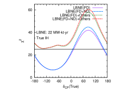
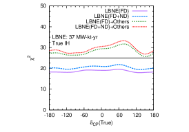
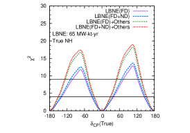
Figure 3.21: Hierarchy/Octant/CP violation discovery sensitivity $\chi^{2}$ vs true $\delta_{CP}$ in the left/middle/right panel. The various curves show the effect of including a near detector on the sensitivity of LBNE alone and LBNE combined with the other experiments.

3.4.2.2 Octant Sensitivity

The mass hierarchy as well as the values of $\delta_{CP}$ and $\theta_{23}$ in nature affect the octant sensitivity of experiments significantly. In our analysis, we have considered various true values of $\delta_{CP}$ across its full range, and two representative true values of $\theta_{23}$ – $39^{\circ}$ and $51^{\circ}$. Having evaluated the minimum $\chi^{2}$ for each of these cases, we have chosen the lower value to get a more conservative estimate. Thus, we have ensured that the adequate exposure shown here holds, irrespective of the true octant of $\theta_{23}$. Note that octant sensitivity reduces as we go more towards $\theta_{23}=45^{\circ}$. Thus the above choice of true $\theta_{23}$ does not correspond to the most conservative case.

The middle panel of Fig. 3.20 shows the combined octant sensitivity of the experiments, as a function of LBNE exposure. Around 35 (37) MW-kt-yr for NH (IH) is the required exposure for LBNE, to measure the octant with NO$\nu$A, T2K and ICAL. This implies a runtime of around 3 years in each mode for the ‘standard’ configuration of LBNE. Without information from ICAL however, LBNE would have to increase its exposure to around 65 (50) MW-kt-yr for NH (IH) to measure the octant with $\chi^{2}=25$. For a 1.2 MW beam and a 10 kt detector this implies about 5 (4) years for NH (IH) in each mode. While only LBNE would need a higher exposure of 84 (76) MW-kt-yr for NH (IH) corresponding to about 7 (6) years in each mode. Thus including ICAL data reduces the exposure required from LBNE. This is summarized in the 2nd row of Table 3.4.

3.4.2.3 Detecting CP Violation

Here, we have tried to determine the fraction of the entire $\delta_{CP}$ range for which the setups can detect CP violation with at least $\chi^{2}=9$. We have always chosen the smallest fraction over the true values of $\theta_{23}$ considered ($39^{\circ}$, $45^{\circ}$ and $51^{\circ}$), so as to get a conservative estimate.

We find in the right panel of Fig. 3.20 that for the range of exposures considered, the fraction of $\delta_{CP}$ is between 0.35 and 0.55. While the exposure increases by a factor of two, the increase in the fraction of $\delta_{CP}$ is very slow. This combination of experiments can detect CP violation over 40% of the $\delta_{CP}$ range with an exposure of about 65 MW-kt-yr at LBNE for NH (i.e. a runtime of around 5.5 years for LBNE). Without including T2K and NO$\nu$A information the exposure required will be 114 MW-kt-yr for 40% coverage for discovery of $\delta_{CP}$. In this context, we want to remind that, one of the mandates of LBNE/DUNE is $3\sigma$ CP coverage for 75% values of $\delta_{CP}$ [90]. We find that an exposure of 300 MW-kt-yr in neutrinos and 300 MW-kt-yr in antineutrinos gives 69% (73%) CP coverage at $3\sigma$ for $\theta_{23}=39^{\circ}$ and 60% (65%) for $51^{\circ}$ in NH (IH). We also find that addition of NO$\nu$A and T2K data does not help much for such high values of exposure. The results are summarized in Table 3.5.

3$\sigma$ CPV coverage for $\theta_{23}$	LBNE	LBNE+NO$\nu$A+T2K
$39^{o}$	69(73)	71(74)
$51^{o}$	60(65)	63(67)

Table 3.5: CPV coverage fraction of LBNE at 3$\sigma$ for total 600 MW-Kt-yr exposure.

In the following subsections, we fix the exposure in each case to be the adequate exposure as listed in Table 3.4, for the most conservative parameter values.

3.4.3 Role of the Near Detector in Reducing Systematics

The role of the near detector (ND) in long-baseline neutrino experiments has been well discussed in the literature, see for example Refs. [194, 195, 196]. The measurement of events at the near and far detector (FD) reduces the uncertainty associated with the flux and cross-section of neutrinos. Thus the role of the near detector is to reduce systematic errors in an oscillation experiment. It has recently been seen that the near detector for the T2K experiment can bring about a spectacular reduction of systematic errors [197].

In this study, we have tried to quantify the improvement in results, once the near detector is included. Instead of putting in reduced systematics by hand, we have explicitly simulated the events at the near detector using GLoBES. The design for the near detector is still being planned. For our simulations, we assume that the near detector has a mass of 5 tons and is placed 459 meters from the source. The flux at the near detector site has been provided by the LBNE collaboration [193]. The detector characteristics for the near detector are as follows [198]. The muon (electron) detection efficiency is taken to be 95% (50%). The NC background can be rejected with an efficiency of 20%. The energy resolution for electrons is $6\%/\sqrt{E\rm{(GeV)}}$, while that for muons is $37$ MeV across the entire energy range of interest. Therefore, for the neutrinos, we use a (somewhat conservative) energy resolution of $20\%/\sqrt{E\rm{(GeV)}}$. The systematic errors that the near detector setup suffers from are assumed to be the same as those of the far detector.

In order to have equal runtime for both FD and ND, we fix the far detector volume as 10 kt and consider both the detectors to receive neutrinos from 1.2 MW beam. This fixes the runtime of FD which is then also used in the simulation for ND. The run times corresponding to the exposures which are taken in this section are following: 1.8 year for hierarchy sensitivity, 3.1 year for octant sensitivity and 5.4 year for CPV discovery sensitivity.

In order to simulate the ND+FD setup for LBNE, we use GLoBES to generate events at both detectors, treating them as separate experiments. We then use these two data sets to perform a correlated systematics analysis using the method of pulls [177]. This gives us the combined sensitivity of LBNE using both near and far detectors. Thereafter, the procedure of combining results with other experiments and marginalising over oscillation parameters continues in the usual manner. The results are shown in Fig. 3.21. The effect of reduced systematic errors is felt most significantly in regions where the results are best. This is because for those values of $\delta_{CP}$, the experiment typically has high enough statistics for systematic errors to play an important role.

Next, we have tried to quantify the reduction in systematic errors seen by the experiment, when the near detector is included. To be more specific, if the systematic errors seen by the far detector setup are denoted by $\vec{\pi}$, then what is the effective set of errors $\vec{\pi}_{\rm eff}$ for the far detector setup, once the near detector is also included. In other words, for given systematic errors $\vec{\pi}$, we have found the value of $\vec{\pi}_{\rm eff}$ that satisfies the relation

$$\chi^{2}({\rm{FD}}(\vec{\pi}_{\rm eff}))\equiv\chi^{2}({\rm{FD}}(\vec{\pi})+{\rm{ND}}(\vec{\pi}))~{},$$ (3.8)

where the right-hand side denotes the correlated combination. The result of the computation is shown in Fig. 3.22, for the case of hierarchy determination. We have chosen typical values of systematic errors for the detector: $\nu_{e}$ appearance signal norm error of 2.5%, $\nu_{\mu}$ disappearance signal norm error of 7.5%, $\nu_{e}$ appearance background norm error of 10% and $\nu_{\mu}$ disappearance background norm error of 15%. The tilt error is taken as 2.5% in both appearance and disappearance channels. The first four numbers constitute $\vec{\pi}$, as labeled in the figure. We have not varied the tilt errors in this particular analysis because their effect on overall results is quite small. The sensitivity of FD+ND obtained using these numbers, are matched by an FD setup with effective errors as follows: $\nu_{e}$ appearance signal norm error of 1%, $\nu_{\mu}$ disappearance signal norm error of 1%, $\nu_{e}$ appearance background norm error of 5% and $\nu_{\mu}$ disappearance background norm error of 5%. Similar results are obtained in the case of octant and CP sensitivity also. These results are summarized in Table 3.6.

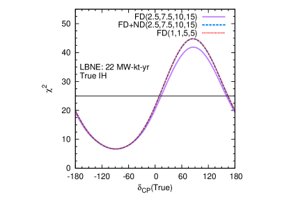
Figure 3.22: $\chi^{2}$ vs $\delta_{CP}$ showing the improvement in systematics due to inclusion of the near detector. The numbers in brackets denote $\nu_{e}$ appearance signal norm error, $\nu_{\mu}$ disappearance signal norm error, $\nu_{e}$ appearance background norm error and $\nu_{\mu}$ disappearance background norm error.

Systematic error	only FD	FD+ND
$\nu_{e}$ app signal norm error	2.5%	1%
$\nu_{\mu}$ disapp signal norm error	7.5%	1%
$\nu_{e}$ app background norm error	10%	5%
$\nu_{\mu}$ disapp background norm error	15%	5%

Table 3.6: Reduction in systematic errors in LBNE with the addition of a near detector.

3.4.4 Significance of the Second Oscillation Maximum

For a baseline of 1300 km, the oscillation probability $P_{\mu e}$ has its first oscillation maximum around 2-2.5 GeV. This is easy to explain from the formula

$$\frac{\Delta_{31}^{(m)}L}{4E}=\frac{\pi}{2}~{},$$

where $\Delta_{31}^{(m)}$ is the matter-modified atmospheric mass-squared difference. In the limit $\Delta_{21}\to 0$, it is given by

$$\Delta_{31}^{(m)}=\Delta_{31}\sqrt{(1-\hat{A})^{2}+\sin^{2}2\theta_{13}}~{}.$$

The second oscillation maximum, for which the oscillating term takes the value $3\pi/2$, occurs at an energy of around 0.6-1.0 GeV. Studies have discussed the advantages of using the second oscillation maximum to get information on the oscillation parameters [199, 200]. In fact, one of the main aims of the proposed ESSnuSB project [94, 201] is to study neutrino oscillations at the second oscillation maximum.

The neutrino flux that LBNE will use has a wide-band profile, which can extract physics from both, the first and second maxima. Fig. 3.23 shows $P_{\mu e}$ for the LBNE baseline, superimposed on the $\nu_{\mu}$ flux. This is in contrast with NO$\nu$A, which uses a narrow-band off-axis beam concentrating on its first oscillation maximum, in order to reduce the $\pi^{0}$ background at higher energies.

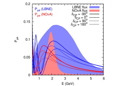
Figure 3.23: Neutrino oscillation probability $P_{\mu e}$ for various representative values of $\delta_{CP}$ and normal hierarchy, for the NO$\nu$A and LBNE baselines. Also shown as shaded profiles in the background are the $\nu_{\mu}$ flux for both these experiments (on independent, arbitrary scales).

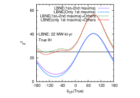
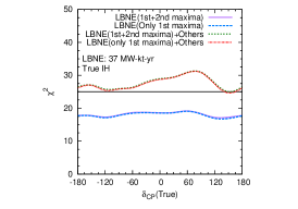
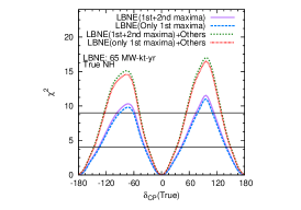
Figure 3.24: Hierarchy/Octant/CP violation discovery sensitivity $\chi^{2}$ vs true $\delta_{CP}$ in the left/middle/right panels respectively. The various curves show the effect of data from the second oscillation maximum on the sensitivity of LBNE alone and LBNE combined with the other experiments.

In order to understand the impact of the second oscillation maximum, we have considered two different energy ranges. Above 1.1 GeV, only the first oscillation cycle is relevant. However, if we also include the energy range from 0.5 to 1.1 GeV, we get information from the second oscillation maximum. Fig. 3.24 compares the sensitivity to the hierarchy, octant and CP violation only from the first oscillation cycle and from both the oscillation cycles assuming the adequate exposures obtained previously. We see that inclusion of data from the second oscillation maximum only increases the $\chi^{2}$ by a small amount. This increase is visible only for hierarchy sensitivity. As expected, the effect is pronounced in the region $\delta_{CP}=-90^{\circ}$. The results for all three performance indicators are given in Table 3.7. It is seen that the effect of including the second oscillation maxima is more for only LBNE for which a higher exposure is needed and this effect is significant for hierarchy sensitivity.

Sensitivity	LBNE+NO$\nu$A+T2K+ICAL		Only LBNE
	1st + 2nd	Only 1st	1st + 2nd	Only 1st
Hierarchy ($\chi^{2}=25$)	22	28	106	218
Octant ($\chi^{2}=25$)	37	39	84	95
CP ($40\%$ coverage	65	70	114	128
at $\chi^{2}=9$)

Table 3.7: Effect of the second oscillation maximum on the sensitivity of LBNE. The numbers indicate the adequate exposure (in MW-kt-yr) required by LBNE for determining the oscillation parameters, with and without the contribution from the second oscillation maximum. For each of the three unknowns, the true parameters (including hierarchy) are taken to be ones for which we get the most conservative sensitivity.

3.4.5 Optimising the Neutrino-Antineutrino Runs

One of the main questions while planning any beam-based neutrino experiment is the ratio of neutrino to antineutrino run. Since the the neutrino and antineutrino probabilities are different due to $\delta_{CP}\rightarrow-\delta_{CP}$, an antineutrino run can provide a different set of data which may be useful in determination of the parameters. However, the interaction cross-section for antineutrinos in the detectors is smaller by a factor of 2.5-3 than the neutrino cross-sections. Therefore, an antineutrino run typically has lower statistics. Thus, the choice of neutrino-antineutrino ratio is often a compromise between new information and lower statistics.

It is well known that neutrino and antineutrino oscillation probabilities suffer from the same form of hierarchy-$\delta_{CP}$ degeneracy [154]. However, the octant-$\delta_{CP}$ degeneracy has the opposite form for neutrinos and antineutrinos [147]. Thus, inclusion of an antineutrino run helps in lifting this degeneracy for most of the values of $\delta_{CP}$ [191]. For measurement of $\delta_{CP}$, it has been shown, for T2K, that the antineutrino run is required only for those true hierarchy-octant-$\delta_{CP}$ combination for which octant degeneracy is present [202]. Once this degeneracy is lifted by including some amount of antineutrino data, further antineutrino run does not help much in CP discovery; in fact it is then better to run with neutrinos to gain in statistics [202]. But this conclusion may change for a different baseline and matter effect. From Fig. 3.23 we see that for NO$\nu$A the oscillation peak does not coincide with the flux peak. Around the energy where the flux peaks, the probability spectra with $\delta_{CP}=\pm 0,180^{\circ}$ are not equidistant from the $\delta_{CP}=\pm 90^{\circ}$ spectra. For antineutrino mode the curves for $\pm 90^{\circ}$ switch position. Hence for neutrinos $\delta_{CP}=0^{\circ}$ is closer to $\delta_{CP}=-90^{\circ}$ and $\delta_{CP}=180^{\circ}$ is closer to $\delta_{CP}=90^{\circ}$, while the opposite is true for antineutrinos. This gives a synergy and hence running in both neutrino an antineutrino modes can be helpful. For T2K the energy where the flux peak occurs coincides with the oscillation peak. At this point the curves for $\delta_{CP}=0,180^{\circ}$ are equidistant from $\delta_{CP}=\pm 90^{\circ}$ and hence this synergy is not present. Thus, the role of antineutrino run is only to lift the octant degeneracy. In what follows we have varied the proportion of neutrino and antineutrino runs to ascertain what is the optimal combination. The adequate exposure is split into various combinations of neutrinos and antineutrinos – 1/6$\ \nu$ + 5/6$\ \overline{\nu}$, 2/6$\ \nu$ + 4/6$\ \overline{\nu}$, … 6/6$\ \nu$ + 0/6$\ \overline{\nu}$. The intermediate configuration 3/6$\ \nu$ + 3/6$\ \overline{\nu}$ corresponds to the equal-run configuration used in the other sections. For convenience of notation, these configurations are referred to simply as 1+5, etc., i.e. without appending the ‘/6’. The results are shown in Fig. 3.25.

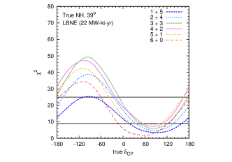
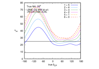
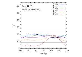
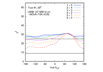
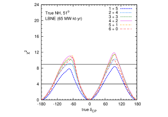
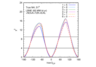
Figure 3.25: Sensitivity of LBNE for various combinations of neutrino and antineutrino run by itself (left panel) and in conjunction with T2K, NO$\nu$A and ICAL (right panel). The top/middle/bottom row shows the sensitivity to hierarchy/octant/CP violation detection. The total exposure has been divided into 6 equal parts and distributed between neutrinos and antineutrinos. For example, for hierarchy sensitivity, 6+0 corresponds to 44 MW-kt-yr in only neutrino; 3+3 correspond to 22 MW-kt-yr in both neutrino and antineutrino mode.

The top row of Fig. 3.25 shows the hierarchy sensitivity of LBNE for various combinations of neutrino and antineutrino run. Normal hierarchy and $\theta_{23}=39^{\circ}$ have been assumed as the true parameters. For LBNE, we have chosen an exposure of 22 MW-kt-yr which was found to be the adequate exposure assuming equal neutrino and antineutrino runs. In the left panel, we see the results for LBNE alone. the figure shows that in the favourable region of $\delta_{CP}\in[-180^{\circ},0]$ the best sensitivity comes from the combination 3+3 or 4+2. Although the statistics is more for neutrinos, the antineutrino run is required to remove the wrong-octant regions. For normal hierarchy, $\delta_{CP}\in[0,180^{\circ}]$ is the unfavourable region for hierarchy determination [154], as is evident from the figure. In this region, we see that the results are worst for pure neutrino run. The best sensitivity comes for the case 5+1. This amount of antineutrino run is required to remove the octant degeneracy. The higher proportion of neutrino run ensures better statistics. In the right panel, along with LBNE we have also combined data from NO$\nu$A, T2K and ICAL. With the inclusion of these data the hierarchy sensitivity increases further and even in the unfavourable region $\chi^{2}=25$ sensitivity is possible with only neutrino run from LBNE. This is because NO$\nu$A, which will run in antineutrino mode for 3 years and the antineutrino component in the atmospheric neutrino flux at ICAL, will provide the necessary amount of information to lift the parameter degeneracies that reduce hierarchy sensitivity. Therefore, the best option for LBNE is to run only in neutrino mode, which will have the added advantage of increased statistics. In the favourable region also the sensitivity is now better for 6+0 and 5+1 i.e. less amount of antineutrinos from LBNE is required because of the antineutrino information coming from NO$\nu$A. Note that overall, the amount of antineutrino run depends on the value of $\delta_{CP}$. However combining information from all the experiments 4+2 seems to be the best option over the largest fraction of $\delta_{CP}$ values.

In the middle row of Fig. 3.25, we have shown the octant sensitivity of LBNE alone (left panel) and in combination with the current experiments (right panel). For LBNE we have used an exposure of 37 MW-kt-yr. We have fixed the true hierarchy to be inverted, and $\theta_{23}=39^{\circ}$ i.e in the lower octant. For this case the probability for neutrinos is maximum for $\delta_{CP}\sim-90^{\circ}$ and overlaps with the higher octant probabilities. Thus the octant sensitivity in neutrino channel is very poor. Thus the worst results for these values of $\delta_{CP}$ come from only neutrino runs. For antineutrino channel because of the flip in $\delta_{CP}$ the probability for $\delta_{CP}=-90^{\circ}$ is well separated from those for HO. Therefore the octant sensitivity comes mainly from antineutrino channel [147]. Thus, addition of antineutrino runs help in enhancing octant sensitivity. Therefore at $-90^{\circ}$ the best sensitivity is from 1+5 i.e $1/6^{th}$ neutrino + $5/6^{th}$ antineutrino combination. On the other hand the neutrino probability is minimum for $\delta_{CP}=+90^{\circ}$ and LO and therefore there is octant sensitivity in the neutrino channel. However since we are considering IH the antineutrino probabilities are enhanced due to matter effect and for a broadband beam some sensitivity comes from the antineutrino channel also. Therefore there is slight increase in octant sensitivity by adding antineutrino data as can be seen. Overall, the best compromise is seen to be reached for 2+4 i.e $1/3^{rd}$ neutrino and $2/3^{rd}$ antineutrino combination, which gives the best results over the widest range of $\delta_{CP}$ values. Addition of NO$\nu$A, T2K and ICAL data increases the octant sensitivity. The octant sensitivity is best for combinations having more antineutrinos. For $\delta_{CP}\sim+90^{\circ}$ all combinations give almost the same sensitivity.

The left and right panels of the bottom row in Fig. 3.25 show the ability of LBNE (by itself, and in conjunction with the current generation of experiment, respectively) to detect CP violation. Here the true hierarchy is NH and true $\theta_{23}$ is $51^{\circ}$. Although this true combination does not suffer from any octant degeneracy, we see in the left panel that 6+0 is not the best combination. This is due to the synergy between neutrino-antineutrino runs for larger baselines as discussed earlier. In both cases, we find that the best option is to run LBNE with antineutrinos for around a third of the total exposure. On adding information from the other experiments, we find great improvement in the CP sensitivity. From the right panel, we see that the range of $\delta_{CP}$ for which $\chi^{2}=9$ detection of CP is possible is almost the same for most combinations of neutrino and antineutrino run. Therefore, as in the case of octant determination, the exact choice of combination is not very important.

3.5 Constraining $\delta_{CP}$ using First Three Years of IceCube Data

In this section, we will try to find constraint on $\delta_{CP}$ by analysing data from ultra high energy neutrinos (UHE) coming from various astrophysical sources. The study of cosmic particles, and through them the study of astrophysical phenomena has gradually moved up the energy scale over the last few decades. The first data set announced by the IceCube collaboration consists of 28 events above 25 TeV, detected over a period of 662 days of live time (May 2011 – May 2012 with 79 strings, and May 2012 – May 2013 with 86 strings). 7 out of these 28 events are tracks signifying ($\nu_{\mu}+\bar{\nu}_{\mu}$) charged-current (CC) events; while the other 21 are showers indicating either ($\nu_{e}+\bar{\nu}_{e}$) or ($\nu_{\tau}+\bar{\nu}_{\tau}$), or ($\nu_{\mu}+\bar{\nu}_{\mu}$) neutral-current (NC) events [203]. This $4\sigma$ detection marked the first discovery of UHE neutrinos. Further data was collected for next one year. For the full 988 days IceCube collected 37 events, adding 1 track, 7 shower events and 1 was produced by a coincident pair of background muons from unrelated air showers that cannot be reconstructed with a single direction and energy.

In this section, we will analyse the IceCube neutrino data to measure $\delta_{CP}$ and determine the source of astrophysical neutrinos. In Ref. [204], the author discussed in detail the complementary nature of astrophysical and terrestrial neutrino experiments in studies regarding the detections of $\delta_{CP}$. In this paper (and more recently in Ref. [205]), data in the form of flavour ratios of observed neutrinos was used. In this study, we have analysed data from IceCube using a similar approach to get a hint about the value of $\delta_{CP}$.

3.5.1 Astrophysical Sources

The data recorded by the IceCube telescope is the first evidence of extra-terrestrial events in the UHE range. These neutrinos can have their origin in extragalactic astrophysical sources like low power Gamma-Ray Burst (GRB) jets in stars [206] or Active Galactic Nuclei (AGN) cores [207]. The energy of the 37 detected neutrino events are in the range $25-2000$ TeV. By tracing the hadronic origin [208] of these events, one can estimate the proton energies at their sources to be within $0.5-40$ PeV. Supernova Remnants (SNRs), AGNs, GRBs and other astrophysical sources can accelerate protons to very high energies. The interactions of these protons with soft photons or matter from the source can give UHE neutrinos through the following process: $p\gamma,pp\rightarrow{\pi^{\pm}}X,\,~{}{\pi^{\pm}}\,\rightarrow\,{\mu^{\pm}}\nu_{\mu}(\bar{\nu}_{\mu}),\,~{}{\mu^{\pm}}\,\rightarrow\,{e^{\pm}}\bar{\nu}_{\mu}(\nu_{\mu})\nu_{e}(\bar{\nu}_{e})$ [209, 210] with a flux ratio of $\phi_{\nu_{e}}:\phi_{\nu_{\mu}}:\phi_{\nu_{\tau}}=1:2:0$ (known as $\pi$S process). Some of the muons, due to their light mass, can get cooled in the magnetic field quickly resulting in a neutrino flux ratio of $0:1:0$ ($\mu$DS process). K-mesons, produced from $p\gamma$ interactions with a cross-section two orders of magnitude less than pions, will cool in the magnetic field of the source at higher energies compared to the pions. $K^{+}\rightarrow{\mu^{+}\bar{\nu_{\mu}}}\,$ is the dominant channel of neutrino production from cooled pions, with a branching fraction of 63%, and with the same flux ratio as the pion decay [211]. The $p\gamma$ interaction also produces high energy neutrons which would decay as $n\,\rightarrow p+e^{-}+\overline{\nu}_{e}$ to antineutrinos [212] with the flux ratio of $1:0:0$ ($n$S process). The relative contribution of each channel depends on different parameters of the astrophysical source like the magnetic field, the strength of the shock wave and density of photon background [213]. Apart from the neutrinos these processes also produce high energy photons inside the source. Correlation of high energy photons with the UHE neutrinos can be considered as a signature of hadron production inside the source. For example, a TeV neutrino can have an accompanying TeV photon at the source. However due to attenuation in the background radiation during propagation, PeV photons will have typical mean free path $\sim 10$ kpc [214]. Thus, the associated photons of TeV neutrinos from extragalactic sources cannot reach earth.

3.5.2 Analysis

The main sources of astrophysical neutrinos are the $\pi$S, $\mu$DS and $n$S channels. However, the exact fraction of events in the detector from each of these sources is not known. Therefore, we have introduced relative fractions $k_{1}$, $k_{2}$ and $k_{3}$ for these three sources respectively, which are treated as free parameters in the problem subject to the normalisation constraint $\sum k_{i}=1$. In this study, we have not considered any other sub-dominant mode of neutrino production.

Neutrinos oscillate during propagation and given that the value of $L/E$ for such neutrinos is very large, we can only observe the average oscillation probability. Therefore, the probabilities take the simple form:

$$P(\nu_{\alpha}\to\nu_{\beta})\equiv P_{\alpha\beta}=\sum_{i}|U_{\alpha i}|^{2}|U_{\beta i}|^{2}~{}.$$ (3.9)

It is worth emphasizing that this oscillation probability depends only on the mixing angles and CP phase, but not on the mass-squared differences. Therefore, unlike in beam-based experiments where knowledge of the mass hierarchy is crucial for CP sensitivity [154], in this case we can (at least in principle) detect CP violation without suffering from the hierarchy degeneracy. Also note that $P_{\alpha\beta}=P_{\beta\alpha}$, therefore the probability can only be an even function of $\delta_{CP}$. As a consequence, we can treat neutrino and antineutrino oscillations on an equal footing. Another consequence of this is that every value of $\delta_{CP}$ allowed by the data will be accompanied by a degenerate solution ($-\delta_{CP}$).

The distinction between tracks (which we assume to be $\nu_{\mu}$ CC events) and showers (which we assume to be $\nu_{e}$ or $\nu_{\tau}$ or $\nu_{\mu}$ NC events) is quite clear in the IceCube detector. We have folded the relative initial fluxes with the oscillation probabilities to get the relative number of events at the detector. Separation of muon events into CC and NC has been done using the ratio of the cross-sections at the relevant energy [215]. We have done a simple analysis using the total events, instead of binning the data in energy and angle. Since the probability is almost independent of energy, this simplification is not expected to affect the analysis. This also allows us to neglect the effect of energy resolution. In Ref. [75], the number of background events in the IceCube data set is estimated to be $10.6^{+5.0}_{-3.6}$. Of these, $6.0\pm 3.4$ are expected to be veto penetrating atmospheric muons and $4.6^{+3.7}_{-1.2}$ are from the atmospheric neutrino background above energy 10 TeV. The background assumed by IceCube could be an overestimation [216], since (a) it has been estimated by extrapolating data, and (b) for atmospheric neutrinos the background has been calculated from 10 TeV while the events have been detected with lowest energy nearly 28 TeV. Therefore, we have used an estimate of 3 background atmospheric muon tracks and 3.4 (the lower limit) background atmospheric neutrinos. IceCube have predicted a total of $8.4\pm 4.2$ muon events and $6.6_{-1.6}^{+5.9}$ atmospheric neutrinos [167] including the next set of neutrino events detected for the period of 988 days. Using the same analysis method we have taken the lowest limit of the backgrounds for our calculation. We have separated the background atmospheric neutrinos into tracks and showers using the same cross-sections as mentioned earlier. These background events are subtracted from the data set in our analysis.

In Refs. [217, 204, 205, 218], the authors have proposed the use of the variable $R={N_{\mu}}/{(N_{e}+N_{\tau})}$ for the study of CP violation with astrophysical sources, where $N_{\alpha}$ is the flux of $\nu_{\alpha}+\bar{\nu}_{\alpha}$ at the detector. This variable helps by eliminating the overall source and detector-dependent normalisation. Moreover, as studies of the up/down ratio as well as data/MC ratio in atmospheric neutrinos have shown, taking ratios of event rates can also reduce the effect of systematics [219, 220]. For our study, we have constructed a similar quantity $\rho={N_{track}}/{N_{shower}}$, with the flavour compositions of the track and shower events as mentioned before.

We have constructed the quantity $\rho^{data}$ using the IceCube data, and calculated $\rho^{theory}$ for a certain value of $\delta_{CP}$ as described above. Background events are subtracted from the data, as mentioned above. The statistical $\chi^{2}$ is then computed using the Gaussian definition

$$\chi^{2}(\delta_{CP})=\left(\frac{\rho^{data}-\rho^{theory}}{\sigma_{\rho}}\right)^{2}~{},$$ (3.10)

where $\sigma_{\rho}$ is the corresponding error . We have incorporated systematic effects using the method of pulls, with a systematic error of 5%. Note that, we have marginalised the $\Delta\chi^{2}$ over the mixing angles ($\theta_{23}$, $\theta_{13}$, $\theta_{12}$) within the ranges $\theta_{23}$ = 35^∘ to 55^∘, $\sin^{2}2\theta_{13}$= 0.085 to 0.115 and $\theta_{12}$= 30^∘ to 36^∘ respectively. Here we take priors on all the three mixing angles. The priors added are $\sigma(\sin^{2}2\theta_{13})$ = 0.01, $\sigma(\sin^{2}2\theta_{23})$ = 0.1 and $\sigma(\sin^{2}\theta_{12})$ = 0.0155.

3.5.3 Results

To demonstrate the impact of the origin of these astrophysical neutrinos on the precision of $\delta_{CP}$, we start with various possibilities, like, single, double or a combination of three sources as the origin. First we show the fit to the data as a function of $\delta_{CP}$ for the single source assumption, in Fig. 3.26.

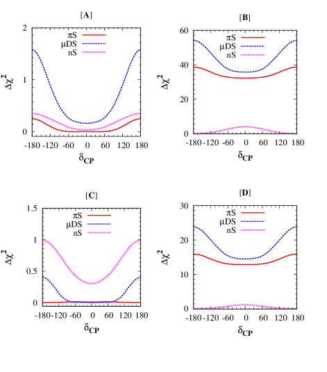
Figure 3.26: Fit to $\delta_{CP}$ considering a single source i.e., $\pi$S ($k_{1}=1,k_{2}=0,k_{3}=0$, solid red), $\mu$DS ($k_{1}=0,k_{2}=1,k_{3}=0$, dashed blue), $n$S ($k_{1}=0,k_{2}=0,k_{3}=1$, dotted magenta), considering all the events being from astrophysical environment. Panel [A]: Three-year data, without background; Panel [B]: Three-year data, with background; Panel [C]: Two-year data, without background; Panel [D]: Two-year data, with background.

The upper row shows the results of our analysis of the full three-year data set. We have also included the results from analysing data from only the first two years (lower row) to show the improvement in results from additional data.

In the left panels we assume that all the events seen at IceCube are purely of astrophysical origin whereas in the right panels we include the effect of backgrounds. The latter is the realistic assumption. From these figures we can see that, in case of no background the $\pi$S source is favoured by the data as compared to the $n$S and $\mu$DS source (though the sensitivity is quite small, as $\Delta\chi^{2}$ is always $\textless$ 1.5). However, when we include the background, the scenario changes completely. Pure $\pi$S and pure $\mu$DS sources are ruled out by the data at $>3\sigma$, while the pure $n$S source is favoured by data, though it is not sufficient to put any significant constraint on the value of $\delta_{CP}$. This has also been pointed out recently in Ref. [216]. This result can be understood qualitatively in the following way. In the 2nd column of Table 3.8 we have listed the theoretically calculated values for track by shower ratio for all the three sources keeping the oscillation parameters fixed at their tri-bimaximal (TBM) values ($\theta_{23}=45^{o}$, $\theta_{13}=0^{o}$, $\sin^{2}\theta_{12}=\frac{1}{3}$) whereas the third column contains the experimental values of the track by shower ratio without and with backgrounds. We can clearly see that for a pure signal, the track to shower ratio for $\pi$S is closest to the data. But the difference becomes quite high when backgrounds are taken under consideration, resulting in a very high $\Delta\chi^{2}$. A comparison of the upper and lower panels shows a marked increase in $\Delta\chi^{2}$. This shows the importance of additional data in both, excluding certain combinations of sources as well as constraining the value of $\delta_{CP}$.

We have also done an analysis of the events in the energy range 60 TeV $<E<$ 3 PeV considering the 3 years of IceCube data. This is motivated by the fact that, this energy interval contains the atmospheric muon background less than one. In this energy range there are 4 track events and 16 shower events with an atmospheric muon background of 0.435 and atmospheric neutrino background of 2.365 [167]. The result is plotted in Fig. 3.27.

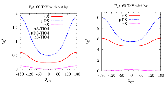
Figure 3.27: Similar plot as that of Fig. 3.26 but for neutrinos within energy 60 TeV to 3 PeV.

In the left panel there is no background and in the right panel background has been considered. From the right panel we can see that we are still getting $n$S as the favoured source whereas $\pi$S and $\mu$DS sources are excluded at more than $2\sigma$. This is due to the fact that though the atmospheric muon background is less than one in this energy range but due to the presence of atmospheric neutrino background $n$S is getting preferred over $\pi$S source. This can bee seen from the left panel where no background is considered. There we can note that the data agrees with the final flavor ratio 1:1:1; i.e., it favours the $\pi$S source over $n$S source marginally when TBM mixing is assumed. But when we vary the oscillation parameters in their allowed $3\sigma$ range then due to the deviation from TBM, $n$S is getting slightly preferred over $\pi$S.

In Fig. 3.28 and Fig. 3.29 we show the fit to the data when neutrinos are coming from two/all the three sources respectively, with equal contributions.

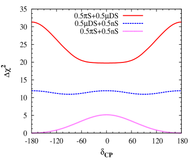
Figure 3.28: Fit to $\delta_{CP}$ considering contribution from two sources at a time, in equal proportion i.e., $k_{1}=k_{2}=0.5,k_{3}=0$ (solid, red), $k_{1}=0,k_{2}=k_{3}=0.5$ (dashed, blue), $k_{1}=k_{3}=0.5,k_{2}=0$ (dotted, magenta).

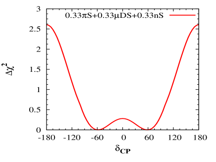
Figure 3.29: Fit to $\delta_{CP}$ considering equal contribution from all the sources, i.e., $k_{1}=k_{2}=k_{3}=0.33$.

These results are for the full data set, and backgrounds have been included in generating these plots. In Fig. 3.28, we find only the combination of $\pi$S and $n$S neutrinos are allowed at $3\sigma$ level. We also see that the CP dependence is maximum if the neutrinos come from the combination of $\pi$S and $\mu$DS modes. The data may also rule out one-third of $\delta_{CP}$ values (approximately $-60^{\circ}$ to $60^{\circ}$) at $\sim 2\sigma$. The poor sensitivity from $n$S neutrinos is the reason why the combination of $\pi$S+$\mu$DS in Fig. 3.28 has a higher $\chi^{2}$ than the combinations involving $n$S. When we consider equal contributions from all these channels (Fig. 3.29), we find that the data favours the first and fourth quadrants of $\delta_{CP}$ at $1\sigma$.

Source	$\frac{N_{track}}{N_{shower}}$(Calculated)	$\frac{N_{track}}{N_{shower}}$(Data)
$\pi$S	0.30
		8/28=0.287(Without background)
$\mu$DS	0.38
		0.05(With background)
$n$S	0.18

Table 3.8: Theoretical values of track by shower ratio for all the three sources along with experimental values with and without background.

We have then performed a check to constrain the astrophysical parameters $k_{i}$ vs $\delta_{CP}$ using the IceCube data, by plotting the allowed contours in the $k_{i}-\delta_{CP}$ plane. In Fig. 3.30, we have showed the $2\sigma$ (light) and $3\sigma$ (dark) contours in the $k_{1}-\delta_{CP}$ plane for three fixed values of $k_{2}$.

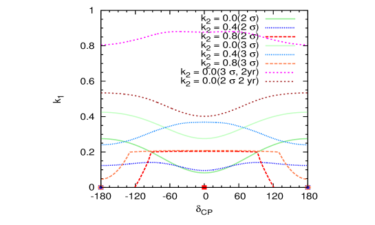
Figure 3.30: Contour plots for allowed region in the $k_{1}-\delta_{CP}$ plane, for three representative values of $k_{2}$. The points marked in the respective colours indicate the best-fit point with new IceCube data.

The best-fit point indicated by the data has been marked with a red dot. We see that the data favours a smaller value of $k_{1}$ and larger values of $k_{2}$ and $k_{3}$. Similarly, Fig. 3.31 shows that for a given value of $k_{1}$, the data disfavours the $\mu$DS process (small value of $k_{2}$) but favours the $n$S process (large value of $k_{3}$).

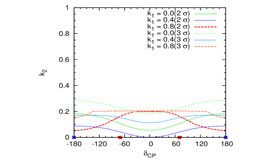
Figure 3.31: Contour plots for allowed region in the $k_{2}-\delta_{CP}$ plane, for three representative values of $k_{1}$. The points marked in the respective colours indicate the best-fit point.

Likewise, Fig. 3.32 shows the data favouring the largest possible value of $k_{3}$ allowed by the normalisation condition.

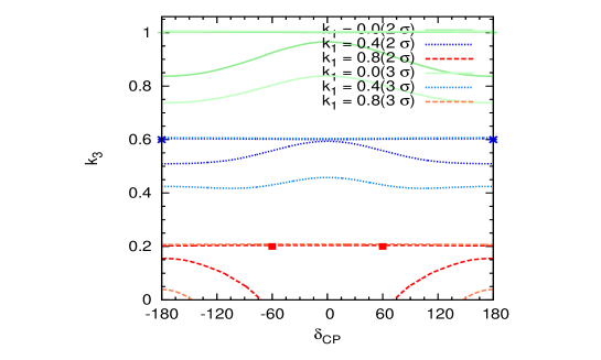
Figure 3.32: Contour plots for allowed region in the $k_{3}-\delta_{CP}$ plane, for three representative values of $k_{1}$. The points marked in the respective colours indicate the best-fit point.

These features can be understood from Fig. 3.26, where we see that the data prefers the $n$S source. From these contours, we may draw certain constraints on the astrophysical sources most favoured. In particular if we obtain a good prior on $\delta_{CP}$ from other experiments, then the most favoured ratio of $k_{1}$, $k_{2}$ and $k_{3}$ may be obtained. Alternately, if we obtain a better picture of the sources of the IceCube events, a refined and constrained range on $\delta_{CP}$ would be predicted.

To show the statistical improvement of the 3 year data over 2 year data, in Fig. 3.30 we have also plotted the $2\sigma$ and $3\sigma$ contours for the latter for $k_{2}=0$. Here we can clearly see that for $\delta_{CP}=0$, 3 year data can exclude $73\%$ ($91.5\%$) of $k_{1}$ values at $3\sigma$ ($2\sigma$) where as the 2 year data can only rule out $13\%$ ($61\%$) of $k_{1}$ values at $3\sigma$ ($2\sigma$). For $\delta_{CP}=\pi$ the exclusion percentages are $58\%$ ($73\%$) at $3\sigma$ ($2\sigma$) for 3 years and $20\%$ ($48\%$) at $3\sigma$ ($2\sigma$) for 2 years. One can understand this qualitatively from the $\pi$S curve of Fig. 3.26 showing a significant improvement in the $\Delta\chi^{2}$ with 3 years of data compared to 2 years.

3.6 Summary

In this chapter we have studied the capabilities of the current/future generation neutrino experiments to constrain the remaining unknowns of neutrino oscillation parameters. In Section 3.2, we have studied the CP sensitivity of the T2K, NO$\nu$A and ICAL@INO experiments. We emphasized the critical impact that atmospheric neutrinos can have in obtaining the first hint of CPV from the LBL experiments T2K/NO$\nu$A. This is achieved by the ability of the atmospheric neutrino data to exclude the degenerate solutions. Taking the projected run times of T2K and NO$\nu$A, we show that adding ICAL data can provide a signature of CPV at $2\sigma$ confidence level for $\sim 58\%$ $\delta_{CP}$ values. We also analyse the synergies between these setups which may aid in CP violation discovery and a precision measurement of $\delta_{CP}$. This has been studied for different combinations of these experiments. We find that, while the CP sensitivity principally arises from the appearance channel of NO$\nu$A/T2K, the appearance and disappearance channels are synergistic due to their different dependences on $\delta_{CP}$. $P_{\mu e}$ depends on $\delta_{CP}$ through the quantity $\cos(\Delta+\delta_{CP})$, while $P_{\mu\mu}$ only has a $\cos\delta_{CP}$ dependence. Thus their combination gives a CP sensitivity significantly higher than the sum of sensitivities of the two channels. We also note that for smaller values of $\theta_{13}$, the CP-discovery $\chi^{2}\propto\theta_{13}$ and hence increases with $\theta_{13}$. On the other hand, for larger values of $\theta_{13}$ the CP-discovery $\chi^{2}\propto(90^{\circ}-\theta_{13})^{2}$ which decreases with $\theta_{13}$. The discovery $\chi^{2}$ attains its highest value in the range $\sin^{2}2\theta_{13}\sim 0.08-0.2$. This tells us that the range of $\theta_{13}$ provided by nature lies in an optimal region which is favourable for CP sensitivity with such experiments.

In Section 3.3 we have studied the physics potential of the LBNO setup to determine neutrino mass hierarchy, octant of $\theta_{23}$ and CP violation in leptonic sector in conjunction with T2K, NO$\nu$A and ICAL. We have explored the minimum exposure needed for such a set-up and quantified the ‘adequate’ configuration that can exclude the wrong hierarchy ($\chi^{2}=25$), exclude the wrong octant ($\chi^{2}=25$) and detect CP violation ($\chi^{2}=9$). We have determined the adequate exposure required for LBNO in units of POT-kt and for the least favourable true hierarchy, $\theta_{23}$ and $\delta_{CP}$. In determining the requisite exposure we fully exploit the possible synergies between the existing LBL experiment T2K and NO$\nu$A  and the atmospheric neutrino experiment ICAL@INO which is likely to commence data taking in five years time. For the prospective LBNO configuration we consider three options: CERN-Pyhäsalmi ($2290$ km) baseline with a LArTPC, CERN-Slanic ($1500$ km) with a LArTPC and CERN-Fréjus ($130$ km) with a Water Čerenkov detector. The ‘adequate’ exposure needed is summarized in Table 3.3 where we give the results for T2K+NO$\nu$A+LBNO with and without ICAL. Inclusion of the atmospheric data from ICAL can play a significant role in reducing the exposure required for hierarchy and octant determination for the 2290 and 1540 km setups and for octant and CP detection for the 130 km set-up. Of the two longer baselines, we find that $2290$ km is best suited to determine the mass hierarchy, while $1540$ km is better for detecting CP violation. However, $130$ km is the best candidate for CP violation physics.

In Section 3.4, we have carried out a similar analysis for the LBNE experiment. We have evaluated the adequate exposure for LBNE (in units of MW-kt-yr), i.e., the minimum exposure for LBNE to determine the unknown parameters in combination with T2K, NO$\nu$A and ICAL, for all values of the oscillation parameters. The threshold for determination is taken to be $\chi^{2}=25$ for the mass hierarchy and octant, and $\chi^{2}=9$ for detecting CP violation. The results are summarized in Table 3.4. We find that adding information from NO$\nu$A and T2K helps in reducing the exposure required by only LBNE for determination of all the three unknowns– hierarchy, octant and $\delta_{CP}$. Adding ICAL data to this combination further help in achieving the same level of sensitivity with a reduction in exposure of LBNE (apart from $\delta_{CP}$). Thus the synergy between various experiments can be helpful in economising the LBNE configuration. We have also probed the role of the near detector in improving the results by reducing systematic errors. We have simulated events at the near and far detectors and performed a correlated systematics analysis of both sets of events. We find an improvement in the physics reach of LBNE when the near detector is included. We have also evaluated the drop in systematics because of the near detector. Our results are shown in Table 3.6.

Further we have checked the role of information from the lowest energy bins which are affected by the second oscillation maximum of the probability. We find that for the combined study of LBNE and the other experiments, the second oscillation maxima do not play much role for the adequate exposure. However for only LBNE, with a higher adequate exposure, the second maxima has a significant role in the hierarchy sensitivity.

Finally, we have done an optimisation study of the neutrino-antineutrino run for LBNE. The amount of antineutrino run required depends on the true value of $\delta_{CP}$. It helps in achieving two objectives – (i) reduction in octant degeneracy and (ii) synergy between neutrino and antineutrino data for octant and CP sensitivity. For hierarchy determination using a total exposure of 44 MW-kt-yr the optimal combination for only LBNE is (3+3) which corresponds to 22 MW-kt-yr in neutrino and antineutrino mode each, for $\delta_{CP}$ in the lower half-plane $[-180^{\circ},0]$ and true NH-LO. For $\delta_{CP}$ in the upper half-plane ($[0,180^{\circ}]$) the optimal ratio is $5/6^{th}$ of the total exposure in neutrinos and + $1/6^{th}$ of the total exposure in antineutrinos. Adding information from T2K, NO$\nu$A and ICAL the best combination for LBNE is $2/3^{rd}$ neutrino + $1/3^{rd}$ antineutrino for $\delta_{CP}$ in the lower half-plane. In the upper half-plane, pure neutrino run gives the best sensitivity. In the latter case, the antineutrino component coming from NO$\nu$A and ICAL helps in reducing the required antineutrino run from LBNE. For octant sensitivity the best result from the combined experiments comes from the proportion $(1/6^{th}+5/6^{th})$ except for $\delta_{CP}=+90^{\circ}$ where all combinations give almost the same sensitivity. For CPV discovery, all combinations give similar results when the data are added together, with equal neutrino and antineutrino or $2/3^{rd}$ neutrino + $1/3^{rd}$ antineutrino combination faring slightly better.

Finally in Section 3.5 we have explored the possibility to constrain the leptonic phase $\delta_{CP}$ from the IceCube data. we have analysed the first IceCube data on TeV-PeV scale neutrinos. We have used the flux ratios of the three neutrino flavours to put constraints on $\delta_{CP}$. We find that the results depend strongly on the source of the neutrinos. After taking into account the effect of backgrounds, we find that the $n$S source of neutrinos is favoured by the data. Depending on the particular combination of sources for these neutrinos, current data can only hint at the allowed region of the $\delta_{CP}$ range. However, we have shown that additional data gives a remarkable improvement in results, which underlines the importance of future data from IceCube. We have also put constraints on the astrophysical parameters $k_{1}$, $k_{2}$ and $k_{3}$ that determine which of the modes of neutrino production is more close to the data.

Chapter 4   Neutrino Mass Matrices

4.1 Overview

In this chapter we discuss the structure of the low energy neutrino mass matrix in the presence of one extra light sterile neutrino. As mentioned in the introduction, the neutrino mass matrix in flavour basis is not diagonal and can be written as

$$M_{\nu} = V^{*}M_{\nu}^{diag}V^{\dagger}$$ (4.1)

where $V$ is the leptonic mixing matrix which contains the neutrino oscillation parameters, in a basis where charged lepton mass matrix is diagonal and $M_{\nu}^{diag}$ is the diagonal mass matrix. From the above equation it is clear that the neutrino oscillation parameters can determine the elements of the low energy neutrino mass matrix $M_{\nu}$. One of the popular themes to study the structure of the low energy mass matrix is in terms of texture zeros. Texture zero means one or more elements of the mass matrix are relatively small compared to the others. Such studies help in understanding the underlying parameter space and the nature of the mass spectrum involved and often predict correlations between various parameters which can be experimentally tested. At the fundamental level the structure of the mass matrix is determined by the Yukawa couplings which are essentially free parameters in most models. Knowing the form of the low energy neutrino mass matrix may help to constrain the high scale structures including zero textures in the Yukawa matrix itself [222, 223, 224, 221]. The origin of texture zero could be due to $U(1)$ symmetry like Froggatt-Neilsen [225] or other flavour symmetries [226], discreet or continuous. Texture zeros in the low energy mass matrices in the context of three generations have been extensively explored both in the quark and lepton sector [227, 228, 229, 230, 231, 232, 233, 234, 235, 236, 237, 238, 239]. In particular for three generations of neutrinos, a very remarkable result was obtained in [228] that there can be at the most two zeros in the low energy neutrino mass matrix in the flavour basis.

As mentioned in the Introduction, data from LSND and MiniBooNE experiments can not be accommodated in the three neutrino scenario. These experiments have reported oscillations which can only be explained by the inclusion of one or more sterile neutrino having mass in the eV scale. The recently observed Gallium and reactor anomaly also provide additional support to the sterile neutrino hypothesis.

These evidences of sterile neutrino motivated us to study the texture zero properties of the neutrino mass matrix in the presence of the light sterile neutrinos and compare the results with that of three generation case. In our study we considered the one-zero and two-zero textures in 3+1 scenario. We find that the allowed textures and correlations between different parameters differ significantly as compared to the results of the three generation case .

This chapter is organised in the following way. In Section 4.2 we will first review and update the texture zero results of the 3 generation case and in section 4.3 we will describe the mass and mixing pattern in the 3+1 scheme. In Section 4.4 and 4.5 we present the results for two-zero and one-zero textures of $M_{\nu}$ in 3+1 scenario. We summarize our results in Section 4.6.

4.2 Texture Zero Results for 3 Generation

In three generation picture, the low energy Majorana neutrino mass matrix $M_{\nu}$ is a $3\times 3$ complex symmetric matrix having six independent elements given by

$$M_{\nu} = \begin{pmatrix}m_{ee}&m_{e\mu}&m_{e\tau}\\ m_{e\mu}&m_{\mu\mu}&m_{\mu\tau}\\ m_{e\tau}&m_{\mu\tau}&m_{\tau\tau}\\ \end{pmatrix}.$$ (4.2)

Thus for three generations there are 15 possible two-zero textures and 6 possible one-zero textures. The two-zero textures are categorised in different classes as shown in Table 4.1.

$A_{1}$	$A_{2}$
$\left(\begin{array}[]{ccc}0&0&\times\\ 0&\times&\times\\ \times&\times&\times\end{array}\right)$	$\left(\begin{array}[]{ccc}0&\times&0\\ \times&\times&\times\\ 0&\times&\times\end{array}\right)$
$B_{1}$	$B_{2}$	$B_{3}$	$B_{4}$
$\left(\begin{array}[]{ccc}\times&\times&0\\ \times&0&\times\\ 0&\times&\times\end{array}\right)$	$\left(\begin{array}[]{ccc}\times&0&\times\\ 0&\times&\times\\ \times&\times&0\end{array}\right)$	$\left(\begin{array}[]{ccc}\times&0&\times\\ 0&0&\times\\ \times&\times&\times\end{array}\right)$	$\left(\begin{array}[]{ccc}\times&\times&0\\ \times&\times&\times\\ 0&\times&0\end{array}\right)$
$C$
$\left(\begin{array}[]{ccc}\times&\times&\times\\ \times&0&\times\\ \times&\times&0\end{array}\right)$
$D_{1}$	$D_{2}$
$\left(\begin{array}[]{ccc}\times&\times&\times\\ \times&0&0\\ \times&0&\times\end{array}\right)$	$\left(\begin{array}[]{ccc}\times&\times&\times\\ \times&\times&0\\ \times&0&0\end{array}\right)$
$E_{1}$	$E_{2}$	$E_{3}$
$\left(\begin{array}[]{ccc}0&\times&\times\\ \times&0&\times\\ \times&\times\end{array}\right)$	$\left(\begin{array}[]{ccc}0&\times&\times\\ \times&\times&\times\\ \times&\times&0\end{array}\right)$	$\left(\begin{array}[]{ccc}0&\times&\times\\ \times&\times&0\\ \times&0&\times\end{array}\right)$
$F_{1}$	$F_{2}$	$F_{3}$
$\left(\begin{array}[]{ccc}\times&0&0\\ 0&\times&\times\\ 0&\times&\times\end{array}\right)$	$\left(\begin{array}[]{ccc}\times&0&\times\\ 0&\times&0\\ \times&0&\times\end{array}\right)$	$\left(\begin{array}[]{ccc}\times&\times&0\\ \times&\times&0\\ 0&0&\times\end{array}\right)$

Table 4.1: Possible two-zero textures in the three generation scenario.

The first analysis of the two-zero textures in the three generation has been done in [228] and shown that among the 15 possible textures, only 7 textures are phenomenologically allowed. A detailed analysis regarding the parameter space of the allowed textures were presented in [229, 230]. At that time $\theta_{13}$ was unknown and those analysis were performed taking the CHOOZ upper bound of $\theta_{13}$. After the precise measurement of $\theta_{13}$, the same analysis has been done by many groups in view of the current data [236, 241, 239]. The main conclusion of the all the analysis are almost same but with the precise measurements of the oscillation parameters the allowed parameter space of the viable textures have been reduced significantly. Below we briefly discuss the main results of the two-zero textures. Textures belonging to $A$ class are allowed in only normal hierarchy. The textures in $B$ class are allowed in both normal and inverted hierarchy. The classes $B1$ and $B4$ predict negative values of $\cos\delta_{CP}$ whereas the classes $B2$ and $B3$ predict positive values of $\cos\delta_{CP}$. The textures belonging to the $B$ class can also predict the octant of $\theta_{23}$. The textures $B1$ and $B3$ predict $\theta_{23}$ in the lower octant and the textures $B2$ and $B4$ predict $\theta_{23}$ in the upper octant for normal hierarchy. The predictions are opposite for the inverted hierarchy. The texture belonging to $C$ class is allowed mainly in the inverted hierarchy. This class is marginally allowed in the normal hierarchy when $\theta_{23}$ is close to $45^{\circ}$. For the viability of this class, when $\theta_{23}<45^{\circ}$, one must have $-90^{\circ}<\delta_{CP}<90^{\circ}$ and when $\theta_{23}>45^{\circ}$, one must have $90^{\circ}<\delta_{CP}<270^{\circ}$. The textures in the classes $D$, $E$ and $F$ are forbidden by the data.

Analysis of the one-zero textures in 3 generations has been done in Ref. [242, 243]. Regarding the matrix element $m_{ee}$ which is the effective mass governing the neutrinoless double beta decay, it is well known that it can vanish only for normal hierarchy. The element $m_{e\mu}$ can be zero in both normal hierarchy and inverted hierarchy. For the case of inverted hierarchy this predicts $\sin\alpha=0$ where $\alpha$ being the Majorana phase. The predictions for $m_{e\tau}=0$ is similar as that of $m_{e\mu}$. The elements $m_{\mu\mu}$ and $m_{\tau\tau}$ can vanish in both the hierarchies. For quasi-degenerate masses i.e., $m_{1}\approx m_{2}\approx m_{3}$, $\theta_{23}$ needs to be below $45^{\circ}$ if $m_{\mu\mu}$ is zero and above $45^{\circ}$ if $m_{\tau\tau}$ is zero. They also predict $\sin\alpha=0$. The element $m_{\mu\tau}$ can only vanish for quasi-degenerate masses and predict $\sin\alpha=0$.

4.3 Masses and Mixing in the 3+1 Scheme

Addition of one extra sterile neutrino to the standard three generation picture gives rise to two possible mass patterns – the 2+2 and 3+1 scenarios [244, 245, 246]. Of these, the 2+2 schemes are strongly disfavored by the solar and atmospheric neutrino oscillation data [247]. The 3+1 picture also suffers from some tension between observation of oscillations in antineutrino channel by LSND and MiniBooNE and non-observation of oscillations in the neutrino channels as well as in disappearance measurements. However, it was shown recently in [248] that a reasonable goodness-of-fit can still be obtained. Although introduction of more than one sterile neutrinos may provide a better fit to the neutrino oscillation data [249, 250], the 3+1 scheme is considered to be minimal and to be more consistent with the cosmological data [251]. Very recently combined analysis of cosmological and short baseline (SBL) data in the context of additional sterile neutrinos have been performed in [253, 252]. The analysis in [253] found a preference of the 3+1 scenario over 3+2 while the analysis in [252] shows that the status of the 3+2 scenario depends on the cosmological data set used and the fitting procedure and no conclusive statement can be made regarding whether it is favored or disallowed.

Theoretically, sterile neutrinos are naturally included in Type-I seesaw model [79, 82]. But their mass scale is usually very high to account for the small mass of the neutrinos. Light sub-eV sterile neutrinos as suggested by the data can arise in many models [112].

Irrespective of the mechanism for generation of neutrino masses the low energy Majorana mass matrix in presence of an extra sterile neutrino will be of dimension $4\times 4$ with ten independent entries and is given as,

$$M_{\nu} = \begin{pmatrix}m_{ee}&m_{e\mu}&m_{e\tau}&m_{es}\\ m_{e\mu}&m_{\mu\mu}&m_{\mu\tau}&m_{\mu s}\\ m_{e\tau}&m_{\mu\tau}&m_{\tau\tau}&m_{\tau s}\\ m_{es}&m_{\mu s}&m_{\tau s}&m_{ss}\\ \end{pmatrix}.$$ (4.3)

There are two ways in which one can add a predominantly sterile state separated by $\sim$ eV² from the standard 3 neutrino mass states. In the first case the additional neutrino can be of higher mass than the other three while in the second case the the fourth neutrino is the lightest state. The later turns out to be incompatible with cosmology since in this case three active neutrinos, each with mass $\sim$ eV results in an enhanced cosmological energy density. Thus it suffices to consider only the first case which admits two possibilities displayed in Fig. 4.1. These are:

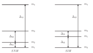
Figure 4.1: The allowed 3+1 mass ordering.

• SNH: in this $m_{1}\approx m_{2}<m_{3}<m_{4}$ corresponding to a normal hierarchy (NH) among the active neutrinos which implies,
  $m_{2}=\sqrt{m_{1}^{2}+\Delta_{21}}~{}~{},m_{3}=\sqrt{m_{1}^{2}+\Delta_{21}+\Delta_{32}}~{}~{},m_{4}=\sqrt{m_{1}^{2}+\Delta_{41}}.$

• SIH : this corresponds to $m_{3}<m_{2}\approx m_{1}<m_{4}$ implying an inverted ordering among the active neutrinos with masses expressed as,
  $m_{1}=\sqrt{m_{3}^{2}+\Delta_{31}}~{}~{},m_{2}=\sqrt{m_{3}^{2}+\Delta_{31}+\Delta_{21}}~{}~{},m_{4}=\sqrt{m_{3}+\Delta_{43}},$

with $\Delta_{ij}=m_{i}^{2}-m_{j}^{2}$. These cases correspond to complete hierarchy among the active neutrinos. The active neutrino mass spectrum can also be quasi-degenerate (QD) where the three active neutrinos have approximately equal masses i.e., SQD: where $|m_{4}|\gg|m_{1}|\approx|m_{2}|\approx|m_{3}|\approx m_{0}$.

In the 3+1 scenario, the neutrino mixing matrix, $V$ in the flavor basis will be a $4\times 4$ unitary matrix. As described in the introduction, in general a N $\times$ N unitary mixing matrix contains $\frac{N(N-1)}{2}$ mixing angles and $\frac{1}{2}(N-1)(N-2)$ Dirac type CP violating phases. It will also have (N-1) number of additional Majorana phases if neutrinos are Majorana particles. So in our case V can be parametrized in terms of sixteen parameters. In addition to the three mixing angles between the active flavors, ($\theta_{13}$, $\theta_{12}$, $\theta_{23}$) we now have three more mixing angles from sterile and active mixing, ($\theta_{14}$, $\theta_{24}$, $\theta_{34}$). There are six CP violating phases, three Dirac ($\delta_{13}$, $\delta_{14}$, $\delta_{24}$) and three additional Majorana phases as ($\alpha$, $\beta$, $\gamma$) as neutrinos here are considered to be Majorana particles. Then, there are four masses of neutrino $m_{1}$, $m_{2}$, $m_{3}$ corresponding to three active states and $m_{4}$ which is predominantly the mass of heavy sterile neutrino.

The mixing matrix $V$ can be expressed as $V=U.P$ [254] where

$$U={R_{34}}\tilde{R}_{24}\tilde{R}_{14}R_{23}\tilde{R}_{13}R_{12},$$ (4.4)

where $R_{ij}$ denotes rotation matrices in the ij generation space and is expressed as,

$R_{34}$=$\left(\begin{array}[]{cccc}1{}&~{}0&0&0\\ 0{}&~{}1&0&0\\ 0{}&~{}0&c_{34}&s_{34}\\ 0{}&~{}0&-s_{34}&c_{34}\end{array}\right)$ , $\tilde{R}_{14}$=$\left(\begin{array}[]{cccc}c_{14}{}&~{}0&~{}~{}0&~{}s_{14}e^{-i\delta_{14}}\\ 0{}&~{}1&~{}~{}0&0\\ 0{}&~{}0&~{}~{}1&0\\ -s_{14}e^{i\delta_{14}}&~{}0&~{}~{}0&c_{14}\end{array}\right)$.

Here we use the abbreviations $s_{ij}=\sin\theta_{ij}$ and $c_{ij}=\cos\theta_{ij}$. The phase matrix is diagonal and is expressed as,

$P=diag(1,e^{i\alpha},e^{i{(\beta+\delta_{13})}},e^{i{(\gamma+\delta_{14})}})$.

4.4 Analysis of Two-Zero Textures

4.4.1 Formalism

The two-zero textures in the neutrino mass matrix give two complex equations viz.

$$M_{\nu(ab)} = 0,$$ (4.5)

$$M_{\nu(pq)} = 0.$$

where a, b, p and q can take the values $e$, $\mu$, $\tau$ and $s$. The above Eq. 4.5 can be written as

$$U_{a1}U_{b1}+\frac{1}{x}U_{a2}U_{b2}+\frac{1}{y}U_{a3}U_{b3}e^{2i\delta_{13}}+zU_{a4}U_{b4}=0,$$ (4.6)

$$U_{p1}U_{q1}+\frac{1}{x}U_{p2}U_{q2}+\frac{1}{y}U_{p3}U_{q3}e^{2i\delta_{13}}+zU_{p4}U_{q4}=0,$$ (4.7)

where

$$x=\frac{m_{1}}{m_{2}}e^{i\alpha},~{}~{}y=\frac{m_{1}}{m_{3}}e^{i\beta},~{}~{}z=\frac{m_{4}}{m_{1}}e^{-2i(\gamma/2-\delta_{14}).}$$ (4.8)

Solving Eqs. (4.6) and (4.7) simultaneously we get the two mass ratios as

$$x=\frac{U_{a3}U_{b3}U_{p2}U_{q2}-U_{a2}U_{b2}U_{p3}U_{q3}}{U_{a1}U_{b1}U_{p3}U_{q3}-U_{a3}U_{b3}U_{p1}U_{q1}+z(U_{a4}U_{b4}U_{p3}U_{q3}-U_{a3}U_{b3}U_{p4}U_{q4})},$$ (4.9)

$$y=-\frac{U_{a3}U_{b3}U_{p2}U_{q2}+U_{a2}U_{b2}U_{p3}U_{q3}}{U_{a1}U_{b1}U_{p2}U_{q2}-U_{a2}U_{b2}U_{p1}U_{q1}+z(U_{a4}U_{b4}U_{p2}U_{q2}-U_{a3}U_{b3}U_{p4}U_{q4})}e^{2i\delta_{13}}.$$ (4.10)

The modulus of these quantities gives the magnitudes $x_{m}$, $y_{m}$ while the argument determines the Majorana phases $\alpha$ and $\beta$.

$$x_{m}=\left|x\right|,~{}~{}y_{m}=\left|y\right|$$ (4.11)

$$\alpha=arg\left(x\right),~{}~{}\beta=arg\left(y\right).$$ (4.12)

Thus, the number of free parameters is five, the lowest mass $m_{1}$ (NH) or $m_{3}$ (IH), three Dirac and one Majorana type CP phases. We can check for the two mass spectra in terms of the magnitude of the mass ratios $x_{m}$, $y_{m}$ and $z_{m}=|z|$ as,

• SNH which corresponds to $x_{m}<1$ , $y_{m}<1$ and $z_{m}>1$.

• SIH which implies $x_{m}<1$ , $y_{m}>1$ and $z_{m}>1$.

Thus, it is $y_{m}$ which determines if the hierarchy among the three light neutrinos is normal or inverted. Note that if the three light neutrinos are quasi-degenerate then we will have $x_{m}\approx y_{m}\approx 1$. Unlike the three generation case, the lowest mass cannot be determined in the four neutrino analysis in terms of $x_{m}$ and $y_{m}$ since these ratios also depend on $m_{1}$ through $z$. Thus, we keep the lowest mass as a free parameter. To find out the allowed two-zero textures we adopt the following procedure.
We vary the lowest mass randomly from 0 to 0.5 eV. The upper limit chosen by us is guided by the cosmological upper bound on neutrino masses. All the five mixing angles (apart from $\theta_{34}$) and the three mass-squared differences are distributed normally about the best-fit values with their corresponding $1\sigma$ errors as given in Table 4.2.

Parameter	Best fit	$1\sigma$ range	$3\sigma$ range
$\Delta_{21}/10^{-5}~{}\mathrm{eV}^{2}$ (NH or IH)	7.54	7.32 – 7.80	6.99 – 8.18
$\sin^{2}\theta_{12}/10^{-1}$ (NH or IH)	3.07	2.91 – 3.25	2.59 – 3.59
$\Delta_{32}/10^{-3}~{}\mathrm{eV}^{2}$ (NH)	2.43	2.33 – 2.49	2.19 – 2.62
$\Delta_{31}/10^{-3}~{}\mathrm{eV}^{2}$ (IH)	2.42	2.31 – 2.49	2.17 – 2.61
$\sin^{2}\theta_{13}/10^{-2}$ (NH)	2.41	2.16 – 2.66	1.69 – 3.13
$\sin^{2}\theta_{13}/10^{-2}$ (IH)	2.44	2.19 – 2.67	1.71 – 3.15
$\sin^{2}\theta_{23}/10^{-1}$ (NH)	3.86	3.65 – 4.10	3.31 – 6.37
$\sin^{2}\theta_{23}/10^{-1}$ (IH)	3.92	3.70 – 4.31	3.35 – 6.63
$\Delta_{LSND}(\Delta_{41}^{2}or\Delta_{43}^{2})~{}\mathrm{eV}^{2}$	0.89	0.80 – 1.00	0.6 – 2
$\sin^{2}\theta_{14}$	0.025	0.018 – 0.033	0.01 – 0.05
$\sin^{2}\theta_{24}$	0.023	0.017 – 0.037	0.005 – 0.076
$\sin^{2}\theta_{34}$	–	–	$<0.16$

Table 4.2: The experimental constraints on neutrino oscillation parameters [127]. The constraints on sterile parameters involving the fourth neutrino are from [253, 255].

The three Dirac and one Majorana type CP phase as well as the remaining mixing angle $\theta_{34}$ are randomly generated. Then, we use the above conditions to find out which mass spectrum is consistent with the particular texture zero structure under consideration. We also calculate the three mass-squared difference ratios

$$R_{\nu} = \frac{\Delta_{21}}{|\Delta_{32}|}=\frac{1-x_{m}^{2}}{|(x_{m}^{2}/y_{m}^{2})-1|},$$

$$R_{\nu 1} = \frac{|\Delta_{31}|}{\Delta_{41}}=\frac{|1-y_{m}^{2}|}{y_{m}^{2}(z_{m}^{2}-1)},$$

$$R_{\nu 2} = \frac{\Delta_{21}}{\Delta_{41}}=\frac{1-x_{m}^{2}}{x_{m}^{2}(z_{m}^{2}-1)}.$$ (4.13)

The $3\sigma$ ranges of these three ratios calculated from the experimental data are

$$R_{\nu} = (0.02-0.04),$$

$$R_{\nu 1} = (1.98\times 10^{-3}-3.3\times 10^{-3}),$$

$$R_{\nu 2} = (0.63\times 10^{-4}-1.023\times 10^{-4}).$$ (4.14)

The allowed textures are selected by checking that they give the ratios within the above range.

4.4.2 Results and Discussions

$A_{1}$	$A_{2}$
$\left(\begin{array}[]{cccc}0&0&\times&\times\\ 0&\times&\times&\times\\ \times&\times&\times&\times\\ \times&\times&\times&\times\end{array}\right)$	$\left(\begin{array}[]{cccc}0&\times&0&\times\\ \times&\times&\times&\times\\ 0&\times&\times&\times\\ \times&\times&\times&\times\end{array}\right)$
$B_{1}$	$B_{2}$	$B_{3}$	$B_{4}$
$\left(\begin{array}[]{cccc}\times&\times&0&\times\\ \times&0&\times&\times\\ 0&\times&\times&\times\\ \times&\times&\times&\times\end{array}\right)$	$\left(\begin{array}[]{cccc}\times&0&\times&\times\\ 0&\times&\times&\times\\ \times&\times&0&\times\\ \times&\times&\times&\times\end{array}\right)$	$\left(\begin{array}[]{cccc}\times&0&\times&\times\\ 0&0&\times&\times\\ \times&\times&\times&\times\\ \times&\times&\times&\times\end{array}\right)$	$\left(\begin{array}[]{cccc}\times&\times&0&\times\\ \times&\times&\times&\times\\ 0&\times&0&\times\\ \times&\times&\times&\times\end{array}\right)$
$C$
$\left(\begin{array}[]{cccc}\times&\times&\times&\times\\ \times&0&\times&\times\\ \times&\times&0&\times\\ \times&\times&\times&\times\end{array}\right)$
$D_{1}$	$D_{2}$
$\left(\begin{array}[]{cccc}\times&\times&\times&\times\\ \times&0&0&\times\\ \times&0&\times&\times\\ \times&\times&\times&\times\end{array}\right)$	$\left(\begin{array}[]{cccc}\times&\times&\times&\times\\ \times&\times&0&\times\\ \times&0&0&\times\\ \times&\times&\times&\times\end{array}\right)$
$E_{1}$	$E_{2}$	$E_{3}$
$\left(\begin{array}[]{cccc}0&\times&\times&\times\\ \times&0&\times&\times\\ \times&\times&\times&\times\\ \times&\times&\times&\times\end{array}\right)$	$\left(\begin{array}[]{cccc}0&\times&\times&\times\\ \times&\times&\times&\times\\ \times&\times&0&\times\\ \times&\times&\times&\times\end{array}\right)$	$\left(\begin{array}[]{cccc}0&\times&\times&\times\\ \times&\times&0&\times\\ \times&0&\times&\times\\ \times&\times&\times&\times\end{array}\right)$
$F_{1}$	$F_{2}$	$F_{3}$
$\left(\begin{array}[]{cccc}\times&0&0&\times\\ 0&\times&\times&\times\\ 0&\times&\times&\times\\ \times&\times&\times&\times\end{array}\right)$	$\left(\begin{array}[]{cccc}\times&0&\times&\times\\ 0&\times&0&\times\\ \times&0&\times&\times\\ \times&\times&\times&\times\end{array}\right)$	$\left(\begin{array}[]{cccc}\times&\times&0&\times\\ \times&\times&0&\times\\ 0&0&\times&\times\\ \times&\times&\times&\times\end{array}\right)$

Table 4.3: Allowed two-zero textures in the 3+1 scenario. The 15 possible two-zero textures of three active neutrinos are same as these after omitting the 4th row and column.

Class	3 gen(Random)	3 gen(Gaussian)	3+1 gen(Gaussian)
A	NH	NH	NH
B	NH, IH, QD	NH($B_{1}$, $B_{3}$), IH($B_{2}$, $B_{4}$)	NH, IH, QD
C	NH, IH, QD	IH	NH, IH, QD
D	-	-	NH, IH
E	-	-	NH, IH
F	-	-	NH, IH,QD

Table 4.4: The allowed mass spectra in 3 and 3+1 scenarios. The last column gives the allowed spectrum for the 3+1 case assuming normal distribution. For random distribution similar mass spectra get allowed although the parameter space is reduced in size. See text for details.

In this section we present the results of our analysis. First we briefly discuss the results that we obtain for the two-zero textures of the $3\times 3$ mass matrices. Next we present the results that we obtain for the 3+1 scenario i.e., $4\times 4$ mass matrices.

4.4.2.1 Results for 3 Active Neutrino Mass Matrix

For the 3 neutrino case, the lowest mass and the two Majorana phases can be determined from the mass ratios. Hence, the only unknown parameter is the Dirac type CP phase ($\delta_{13}$) which is generated randomly. All the other oscillation parameters are distributed normally, peaked at the best-fit and taking their one sigma error as width.

In our analysis, we find that all 7 textures which were allowed previously (as discussed in section 4.2) remain so. However, the textures belonging to A class allow NH whereas for the B class, $B_{1}$ and $B_{3}$ admit NH and $B_{2}$ and $B_{4}$ allow IH solutions. Class C gets allowed only for IH. The D, E and F classes remain disallowed. This is summarized in the second column of Table 4.4. We also display the results that we obtain for the two-zero neutrino mass matrices with three active neutrinos using random distribution of the oscillation parameters. The results obtained in this case are somewhat different from that obtained using normal distribution of oscillation parameters. The reason for the difference stems from the different range of values of the atmospheric mixing angle $\theta_{23}$ used by these methods. If we assume a Gaussian distribution for $\sin^{2}\theta_{23}$ around its best-fit then there is very less probability of getting the 3$\sigma$ range in the higher octant as these values lie near the tail of the Gaussian distribution. This disallow $B_{2}$ and $B_{4}$ for NH and $B_{1}$ and $B_{3}$ for IH [236]. Similarly QD solutions for B class requires $\theta_{23}\sim\pi/4$ [228] and for a normal distribution of $\theta_{23}$ with the peak at present best-fit the 3$\sigma$ range extends up to $\sim 44^{o}$ and there is very little probability of getting values close to $45^{\circ}$. Similarly for the C class NH and QD solutions are allowed only for $\theta_{23}$ values close to $45^{\circ}$ and hence is not admissible when Gaussian distribution of oscillation parameters about the best-fit value is assumed.

4.4.2.2 Results for 3+1 Scenario

Adding one sterile neutrino, there exist in total forty five texture structures of the neutrino mass matrix which can have two zeros.

1. Among these the 9 cases with $|m_{ss}|$= 0 eV are disallowed as the mass matrix element $m_{ss}$ contains the term $m_{4}U_{s4}^{2}$ which is large from the current data and suppresses the other terms. Hence, $|m_{ss}|$ cannot vanish.

2. There are 21 cases where one has at least one zero involving the mass matrix element of the sterile part i.e., $|m_{ks}|$ =0 eV where $k=e,\mu,\tau$. This element is of the form,

   $$m_{ks} = m_{1}U_{k1}U_{s1}+m_{2}U_{k2}U_{s2}e^{-i\alpha}$$

   $$+ m_{3}U_{k3}U_{s3}e^{i(2\delta_{13}-\beta)}+m_{4}U_{k4}U_{s4}e^{i(2\delta_{14}-\gamma)}.$$

   The last term in this expression contains the product $m_{4}U_{s4}$ which is mostly large as compared to first three terms and thus, there can be no cancellations. However, it is possible that in the regime where the active neutrinos are quasi-degenerate, their contribution can match the contribution from the sterile part. But we have checked that in any case, it is not possible to obtain a two-zero texture with these elements. Thus we can exclude these 21 cases from the allowed two-zero textures.

   We will elaborate these points further in the next section at the time of discussing one zero texture.

3. The remaining cases are the 15 two-zero cases for which none of the sterile components are zero. Thus, these also belong to the two-zero textures of the three generation mass matrix. A general element in this category can be expressed as,

   $$m_{kl} = m_{1}U_{k1}U_{l1}+m_{2}U_{k2}U_{l2}e^{-i\alpha}$$

   $$+ m_{3}U_{k3}U_{l3}e^{i(2\delta_{13}-\beta)}+m_{4}U_{k4}U_{l4}e^{i(2\delta_{14}-\gamma)}.$$

   here, $k,l=e,\mu,\tau$. We find all these 15 textures, presented in Table 4.3 get allowed with the inclusion of the sterile neutrino. This can be attributed to additional cancellations that the last term in Eq. (iii) induces. Table 4.4 displays the nature of the mass spectra that are admissible in the allowed textures.

   

   

   

   

   

   

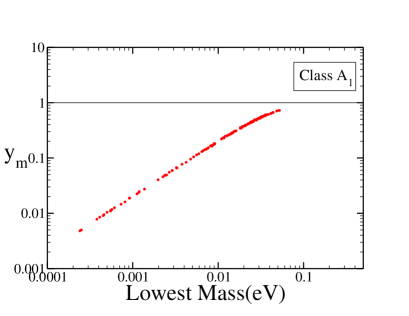
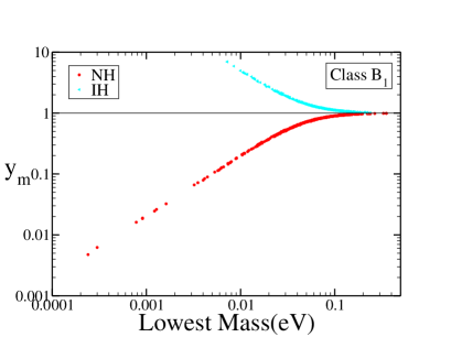
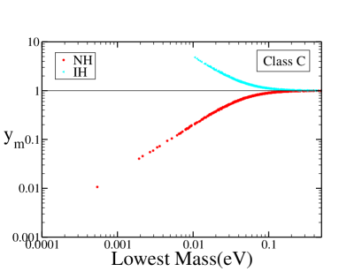
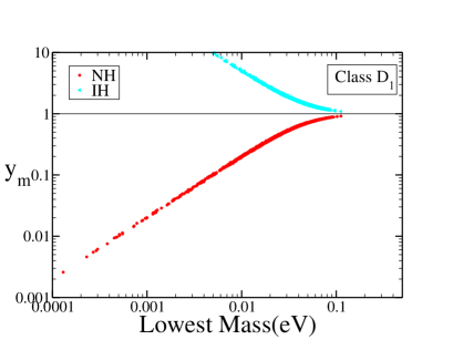
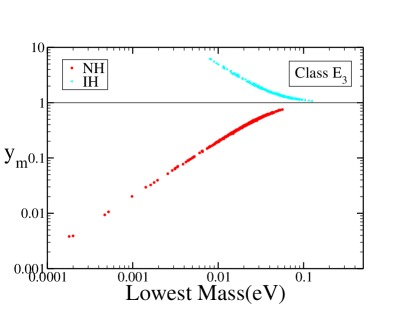
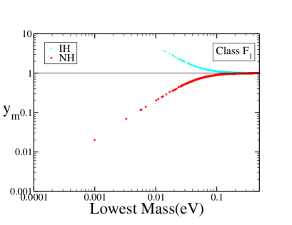
   Figure 4.2: The values of $y_{m}$($=\frac{m_{1}}{m_{3}}$) as a function of the lowest mass ($m_{1}$ or $m_{3}$) for the 3+1 case when the known oscillation parameters are varied in Gaussian distributions peaked at their respective best-fit values.

   In Fig. 4.2 we present the values of $y_{m}$ vs the lowest mass for representative textures $A_{1}$, $B_{1}$, $C$, $D_{1}$, $E_{3}$ and $F_{1}$ from the 6 classes. The other textures belonging to each class give similar results. This figure shows that for textures belonging to the A class $y_{m}$ remains $<$ 1. Thus, it admits only NH solutions. The textures belonging to the D and E class allow NH and IH while the B, C, and F classes allow NH, IH and QD mass spectra.

   The textures $A_{1}-A_{2}$, $B_{1}-B_{2}$, $B_{3}-B_{4}$, $D_{1}-D_{2}$, $E_{1}-E_{2}$ and $F_{2}-F_{3}$ are related by $S_{\mu\tau}$ symmetry where for the four neutrino framework $S_{\mu\tau}$ can be expressed as,

   $S_{\mu\tau}=\left(\begin{array}[]{cccc}1&0&0&0\\ 0&0&1&0\\ 0&1&0&0\\ 0&0&0&1\end{array}\right)$

   in such a way that

   $A_{2}=S_{\mu\tau}^{T}A_{1}S_{\mu\tau}.$

   Note that for 3 generation case the angle $\theta_{23}$ in the partner textures linked by $\mu-\tau$ symmetry was related as $\bar{\theta}_{23}=(\frac{\pi}{2}-\theta_{23})$. However, for the 3+1 case no such simple relations are obtained for the mixing angle $\theta_{23}$. The angles $\theta_{24}$ and $\theta_{34}$ in the two textures related by $\mu-\tau$ symmetry are also different. For this case, the mixing angles for two textures linked by $S_{\mu\tau}$ symmetry are related as

   $$\bar{\theta}_{12} = \theta_{12},~{}~{}~{}\bar{\theta}_{13}=\theta_{13},~{}~{}~{}\bar{\theta}_{14}=\theta_{14},$$ (4.17)

   $$\sin{\bar{\theta}_{24}} = \sin\theta_{34}\cos{\theta_{24}},$$ (4.18)

   $$\sin{\bar{\theta}_{23}} = \frac{\cos{\theta_{23}}\cos{\theta_{34}}-\sin{\theta_{23}}\sin{\theta_{34}}\sin{\theta_{24}}}{\sqrt{1-\cos{\theta_{24}^{2}}\sin{\theta_{34}^{2}}}},$$ (4.19)

   $$\sin{\bar{\theta}_{34}} = \frac{\sin{\theta_{24}}}{\sqrt{1-\cos{\theta_{24}^{2}}\sin{\theta_{34}^{2}}}}.$$ (4.20)

The texture zero conditions together with the constraints imposed by the experimental data allow us to obtain correlations between various parameters specially the mixing angles of the 4^th neutrino with the other three for the A and E classes. For the B, C, D and F classes one gets constraints on the effective mass governing $0\nu\beta\beta$.

In order to gain some analytic insight into the results it is important to understand the mass scales involved in the problem. The solar mass scale is $\sqrt{\Delta_{21}}\approx 0.009$ eV whereas the atmospheric mass scale is $\sqrt{\Delta_{31}}\approx 0.05$ eV. Normal hierarchy among the active neutrinos implies $m_{1}<<m_{2}<<m_{3}$ corresponding to $m_{1}\ \hbox to0.0pt{\raise 2.0pt\hbox{$<$}\hss}{\lower 2.0pt\hbox{$\sim$}}\ 0.009$ eV. It is also possible that $m_{1}\approx m_{2}<<m_{3}$ implying $m_{1}\sim$ (0.009-0.1) eV. We call this partial normal hierarchy. IH corresponds to $m_{3}<<m_{1}\approx m_{2}$. If on the other hand $m_{1}>$ 0.1 eV then $m_{1}\approx m_{2}\approx m_{3}$ which corresponds to quasi-degenerate neutrinos.

• $A$ and $E$ Class

  

  

  

  

  

  

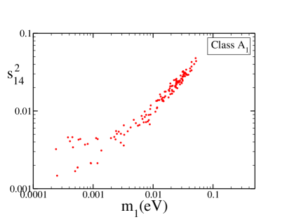
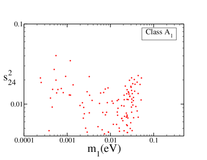
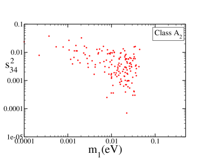
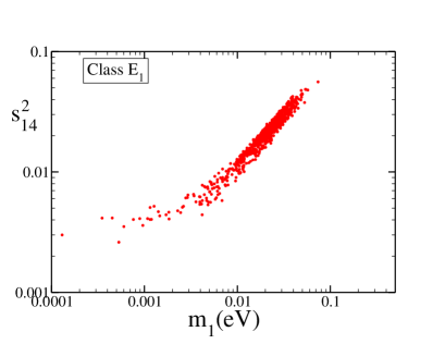
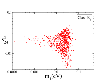
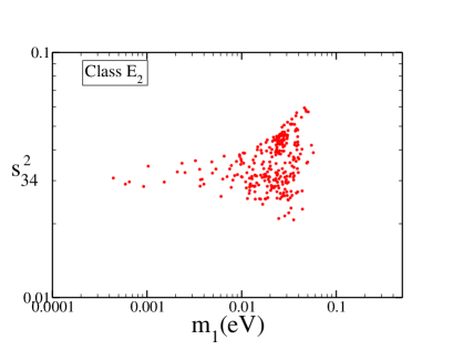
  Figure 4.3: Correlation plots for $A$ and $E$ class.

  For these classes we find $y_{m}$ to be mainly in the range $>$ 0.0001 eV extending up to $\sim 0.1$ eV. Thus, these classes allow normal hierarchy (full or partial) among the 3 active neutrinos. These classes are characterised by the condition $|m_{ee}|=0$. $m_{ee}$ for the four neutrino framework can be expressed as,

  $$m_{ee} = c_{12}^{2}c_{13}^{2}c_{14}^{2}m_{1}+c_{13}^{2}c_{14}^{2}e^{-i\alpha}{m_{2}}s_{12}^{2}$$

  $$+ c_{14}^{2}e^{-i\beta}m_{3}s_{13}^{2}+e^{-i\gamma}{m_{4}}s_{14}^{2}.$$

  For smaller values of $m_{1}$ and NH, the dominant contribution to the magnitude of the above term is expected to come from the last term $s_{14}^{2}\sqrt{\Delta_{41}}\sim 0.022$. Therefore, very small values of $m_{1}$ is less likely to give vanishing $m_{ee}$ for normal hierarchy. However, we get some allowed points in the small $m_{1}$ regime which implies smaller values of $s_{14}^{2}$. $m_{ee}$ can be approximated in the small $m_{1}$ limit as,

  $$m_{ee}\approx e^{-i\alpha}{m_{2}}s_{12}^{2}+e^{-i\beta}m_{3}s_{13}^{2}+e^{-i\gamma}{m_{4}}s_{14}^{2}.$$ (4.22)

  The maximum magnitude of the first two terms is $\sim 0.003$. Then using typical values of $m_{4}$ ($\sim$ 0.9 eV) from the 3$\sigma$ range, we obtain $s_{14}^{2}\sim(0.003-0.004$) in the small $m_{1}$ limit. This is true for all the textures in the A and E class. For the $A_{1}$ class we also simultaneously need vanishing $|m_{e\mu}|$. In the small $m_{1}$ limit approximate expression for $m_{e\mu}$ is

  $$m_{e\mu} \approx e^{i(\delta_{14}-\delta_{24}-\gamma)}s_{14}s_{24}m_{4}$$

  $$+ e^{i(\delta_{13}-\beta)}s_{13}s_{23}m_{3}+e^{-i\alpha}c_{12}c_{23}s_{12}m_{2},$$

  and the first term i.e., $m_{4}s_{14}s_{24}\sim(0.05-0.06)s_{24}$. While the other terms are of the order (0.006 - 0.007) which implies $s_{24}^{2}\sim(0.01-0.02)$. This is reflected in the first and second panels of Fig. 4.3 where the correlation of $s_{14}^{2}$ and $s_{24}^{2}$ with $m_{1}$ is depicted. As $m_{1}$ increases the contribution from the first three terms in $m_{ee}$ increases and $s_{14}^{2}$ becomes larger for cancellation to occur. For $m_{e\mu}$, this increase in $s_{14}$ helps to achieve cancellation for higher values of $m_{1}$ and therefore $s_{24}^{2}$ stays almost the same. Similar argument also apply to the $E_{1}$ class which has vanishing $m_{\mu\mu}$.

  For $A_{2}$ class, in addition we have vanishing $m_{e\tau}$. In the limit of small $m_{1}$, $m_{e\tau}$ can be approximated as,

  $$m_{e\tau}\approx e^{i(\delta_{14}-\delta_{24}-\gamma)}s_{14}s_{34}m_{4}+e^{i(\delta_{13}-\beta)}s_{13}^{2}m_{3}-m_{2}e^{-i\alpha}s_{12}c_{12}s_{23}.$$ (4.24)

  As discussed earlier vanishing $m_{ee}$ implies small $s_{14}^{2}\sim(0.002-0.005$) in the limit of small $m_{1}$. Thus, the contribution from the $m_{4}$ term is $\sim(0.04-0.06)s_{34}$. The typical contribution from the last two terms is $\sim 0.008$. This implies $s_{34}^{2}$ to be in the range (0.02 -0.04) for smaller values of $m_{1}$. This is reflected in the third panels of Fig. 4.3 where we have plotted the correlation of $s_{34}^{2}$ with $m_{1}$. Since with increasing $m_{1}$, $s_{14}$ increases to make $|m_{ee}|=0$, $s_{34}^{2}$ does not increase further. Similar bounds on $s_{34}^{2}$ are also obtained for $E_{2}$ class.

  As one approaches the QD regime then the terms containing the active neutrino masses starts contributing more. So for higher values of $m_{1}$ complete cancellation leading to vanishing $m_{ee}$ even at the highest value of $s_{14}^{2}$ is not possible. This feature restricts $m_{1}$ to be $<$ 0.1 eV in A class.

  Textures belonging to A and E class contain banishing $m_{ee}$ which is not possible for IH in the three generation case since the solar mixing angle is not maximal. In the 3+1 scenario a cancellation leading to vanishing $m_{ee}$ is possible for IH. In this case, the condition $m_{ee}=0$ constraints the majorana phases as $80^{o}<\alpha<280^{o}$, $160^{o}<\gamma<220^{o}$ and the 1-4 mixing angle as $s_{14}^{2}$ as $0.017<s_{14}^{2}<0.042$. These conditions are not compatible with the condition of vanishing $m_{e\mu}$ or $m_{e\tau}$ for IH. Therefore, class A which simultaneously requires one of these elements to vanish along with $m_{ee}$ is disfavoured for IH. On the other hand, the elements i.e., $m_{\mu\mu}$, $m_{\mu\tau}$ or $m_{\tau\tau}$ can assume zero value satisfying these constraints. Thus E class which has $m_{ee}$ together with one of these elements as vanishing can have inverted hierarchical spectrum.

  For vanishing $m_{ee}$, the effective mass ($m_{eff}$ = $|m_{ee}|$) governing the neutrinoless double beta decay ($0\nu\beta\beta$) is also vanishing for these classes.

  

  

  

  

  

  

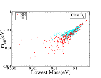
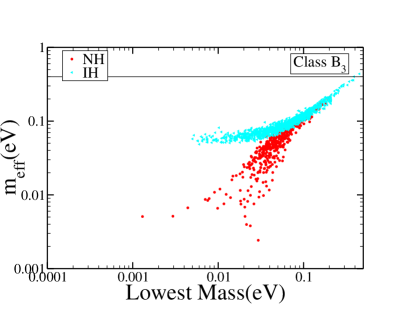
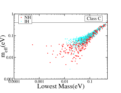
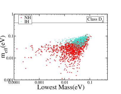
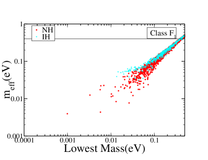
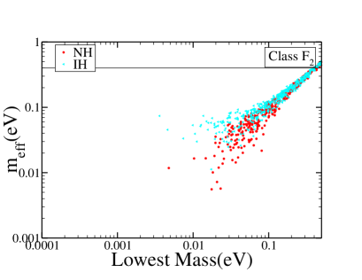
  Figure 4.4: The effective mass governing $0\nu\beta\beta$ as a function of the lowest mass. The red (dark) points correspond to NH while the cyan (light) points correspond to IH. The horizontal line is the current bound from neutrinoless double-beta decay experiments.

• $B,C$ Classes

  In the 3+1 scenario, B and C classes allow all three mass spectra – NH, IH and QD assuming the known oscillation parameters to be normally distributed (cf. Table 4.4). In this case since $\theta_{23}$ in the textures related by $\mu-\tau$ symmetry is not correlated in a simple way, the value of this angle not being in the higher octant does not play a significant role as in the 3 generation case. Among these only $B_{1}$ allow few points for smaller values of $m_{1}$ for NH. For the IH solution, larger number of points are obtained corresponding to the lowest mass $>$ 0.01 eV as is seen from Fig. 4.2. In these textures, for higher values of the lowest mass the active neutrino contribution to the matrix elements are larger and it is easier to obtain cancellations. Hence, textures belonging to these classes show a preference for QD solutions. For these textures the effective mass governing $0\nu\beta\beta$ is non-zero. In the first row of Fig. 4.4 we present the effective mass as a function of the lowest mass for the textures $B_{1}$, $B_{3}$ and C for both NH and IH. These two merge at higher values of the lowest mass corresponding to the QD solution. The effective mass in these textures is $>0.002$ eV for NH and $>$ 0.02 eV for IH. If no signal is seen in future $0\nu\beta\beta$ experiments then large part of the parameter space belonging to these textures can be disfavoured.

• $D,F$ Classes

  These two textures are disallowed in the three generation case. However for the 3+1 scenario they get allowed. NH is admissible in all the textures belonging to these classes. The reason for this is the following.
  In the three active neutrino scenario, the neutrino mass matrix in a $\mu-\tau$ block has the elements of the order of $\sqrt{\Delta_{32}}\approx{0.01}eV$ for normal hierarchy. Thus, in general these elements are quite large and cannot vanish [228]. However, in the 3+1 case when there is one additional sterile neutrino, the neutrino mass matrix elements get contribution from the sterile part of the form $m_{4}U_{k4}U_{l4}$ where $k=e,\mu,\tau$. This term is almost of the same order of magnitude and thus can cancel the active part, resulting into the possibility of vanishing elements in the $\mu-\tau$ block. Thus, the zero textures which were disallowed for NH are now allowed by the inclusion of sterile neutrino (3+1 case). In the case of IH, $m_{\mu\tau}$ element for three active neutrinos is always of the order of $\sqrt{\Delta_{32}}\approx{0.01}eV$ and thus the textures $D_{1}$, $D_{2}$, $F_{2}$, $F_{3}$ which requires $m_{\mu\tau}$ to vanish, were not allowed. However, for the 3+1 scenario the extra term coming due to the fourth state helps in additional cancellations and IH gets allowed in these (cf. Table 4.4). For $F_{1}$ class, IH for three active neutrino is disfavored because of phase correlations. However, with the additional sterile neutrino this can be evaded making it allowed. In the bottom row of Fig. 4.4 we present the effective mass governing $0\nu\beta\beta$ for the textures $D_{1}$, $F_{1}$ and $F_{2}$ as a function of the lowest mass. The texture $D_{1}$ allows lower values of $m_{1}$ for NH while for IH the lowest mass is largely $\ \hbox to0.0pt{\raise 2.0pt\hbox{$>$}\hss}{\lower 2.0pt\hbox{$\sim$}}\ 0.01$ eV. QD solution is not allowed in D class . For F class more points are obtained in the QD regime. Future experiments on $0\nu\beta\beta$ would be able to probe these regions of parameter space.

The results presented above are obtained by varying the known oscillation parameters distributed normally around their best-fit and with a width given by the 1$\sigma$ range of the parameters. There is a finite probability of getting the points in the 3$\sigma$ range of this Gaussian distribution although more points are selected near the best-fit values. However, note that for some of the parameters the 3$\sigma$ range obtained in this procedure is different from the $3\sigma$ range of the global fits. Thus, our results may change if we vary the parameters randomly in their 3$\sigma$ range as we have seen in the 3 generation case. In Fig. 4.5 we show the allowed values of $y_{m}$ as a function of the lowest mass for the case where all the parameters are varied randomly in their 3$\sigma$ range. We find that lower values of the smallest mass get disfavored by this method. The main reason for this is that if we use the Gaussian method then the allowed 3$\sigma$ range of the mixing angle $s_{14}^{2}$ is from (0.002 - 0.048) while that of $s_{24}^{2}$ is from (0.001 - 0.06). Thus, smaller values of $s_{14}^{2}$ and $s_{24}^{2}$ are possible which helps in achieving cancellation conditions for smaller values of $m_{1}$ or $m_{3}$. But if the parameters are varied randomly in the 3$\sigma$ range then such smaller values of the angles are not allowed and consequently no allowed points are obtained for smaller values of masses. In particular, we obtain $m_{1}$ (NH) or $m_{3}$ (IH) $>$ 0.01 eV in all the textures. However, main conclusions presented in Table 4.4 regarding the nature of the allowed mass spectrum for the 3+1 scenario remain unchanged though the allowed parameter space gets reduced. Specially for the A, E and C classes very few points get allowed. Fully hierarchical neutrinos ($m_{1}<m_{2}<m_{3}$) are not possible in any of the textures. Textures belonging to the B and F classes give more points in the QD regime. D class allows partial NH or IH.

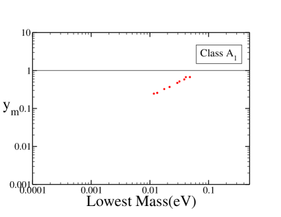
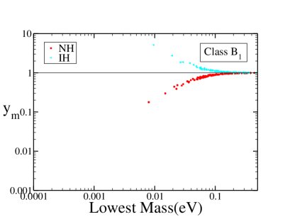
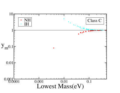
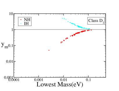
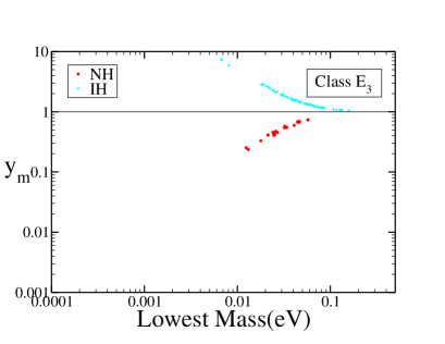
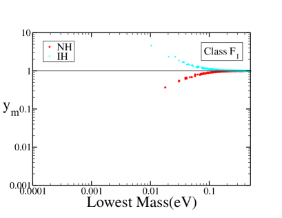
Figure 4.5: The values of $y_{m}$ as a function of the lowest mass when parameters are varied randomly.

4.5 Analysis of One-Zero Textures

4.5.1 Formalism

For the analysis of the one-zero textures of $M_{\nu}$, we define the ratio of the mass squared differences $\xi$ and $\zeta$ as

$$\xi=\frac{\Delta_{41}}{\Delta_{32}}~{}~{}({\rm NH})~{}~{}\text{or}~{}~{}\frac{\Delta_{43}}{\Delta_{31}}~{}~{}({\rm IH}),~{}~{}$$ (4.25)

$$\zeta=\frac{\Delta_{21}}{\Delta_{32}}~{}~{}({\rm NH})~{}~{}{\rm or}~{}~{}\frac{\Delta_{21}}{\Delta_{31}}~{}~{}({\rm IH}).$$ (4.26)

In the extreme cases and using $\zeta\ll 1$, these masses can be written in terms of $\xi$ and $\zeta$ as

$$SNH:|m_{4}|\approx\sqrt{\Delta_{32}\xi}\gg|m_{3}|\approx\sqrt{(1+\zeta)\Delta_{32}}\approx\sqrt{\Delta_{32}}\gg|m_{2}|\approx\sqrt{\Delta_{32}\zeta}\gg|m_{1}|,$$ (4.27)

$$SIH:|m_{4}|\approx\sqrt{\Delta_{31}\xi}\gg|m_{2}|\approx\sqrt{(1+\zeta)\Delta_{31}}\approx\sqrt{\Delta_{31}}\approx|m_{1}|\gg|m_{3}|,$$ (4.28)

$$SQD:~{}~{}|m_{4}|\gg|m_{1}|\approx|m_{2}|\approx|m_{3}|\approx m_{0}.$$ (4.29)

4.5.2 Neutrino Mass Matrix Elements

In this section we study the implication of the condition of vanishing $m_{\alpha\beta}$ for the 3+1 scenario, where $\alpha,\beta=e,\mu,\tau,s$. Since $m_{\alpha\beta}$ is complex the above condition implies both real and imaginary parts are zero. Therefore to study the one-zero textures we consider $|m_{\alpha\beta}|=0$. The best-fit values and the 3$\sigma$ ranges of the sterile neutrino parameters which we have used in this part our analysis are given in Table 4.5 where we also present the mass ratios $\zeta$ and $\xi$ which would be useful in our analysis. For the oscillation parameters involving the active neutrinos we use the global analysis results of Ref. [127] which we also used in our analysis of two-zero textures (presented in Table 4.2).

Parameter	Best Fit values	$3\sigma$ range
$\Delta_{{\rm LSND}}~{}\mathrm{eV}^{2}$	1.62	0.7 – 2.5
$\sin^{2}\theta_{14}$	0.03	0.01 – 0.06
$\sin^{2}\theta_{24}$	0.01	0.002 – 0.04
$\sin^{2}\theta_{34}$	–	$<$ 0.18
$\zeta/10^{-2}$ (NH)	–	2.7 – 3.7
$\zeta/10^{-2}$ (IH)	–	2.7 – 3.8
$\xi/10^{3}$ (NH)	–	0.27–1.14
$\xi/10^{3}$ (IH)	–	0.27– 1.15

Table 4.5: The constraints on sterile neutrino parameters are from [256, 255], where $\Delta_{{\rm LSND}}=\Delta_{41}({\rm NH})$ or $\Delta_{43}({\rm IH})$. Also given are the $3\sigma$ ranges of the mass ratios $\zeta$ and $\xi$.

In this part of the analysis we have varied all the parameters randomly between their allowed ranges, three Dirac phases in the range 0 to $2\pi$ and the three Majorana phases from 0 to $\pi$.

4.5.2.1 The Mass Matrix Element $m_{ee}$

The matrix element $m_{ee}$ in the 3+1 scenario is given as,

$$m_{ee}=m_{1}c_{14}^{2}c_{13}^{2}c_{12}^{2}+m_{2}s_{12}^{2}c_{14}^{2}c_{13}^{2}e^{2i\alpha}+m_{3}s_{13}^{2}c_{14}^{2}e^{2i\beta}+m_{4}s_{14}^{2}e^{2i\gamma}.$$ (4.30)

This is of the form

$$m_{ee}=c_{14}^{2}(m_{ee})_{3\nu}+e^{2i\gamma}s_{14}^{2}m_{4},$$ (4.31)

where $(m_{ee})_{3\nu}$ corresponds to the matrix element in the 3 active neutrino case. The contribution of the sterile neutrino to the element $m_{ee}$ depends on the mass $m_{4}$ and the active-sterile mixing angle $\theta_{14}$. Of all the mass matrix element $m_{ee}$ has the simplest form because of the chosen parametrization and can be understood quite well. Using approximation in Eq. 4.27 for the case of extreme hierarchy one can write this for NH as,

$$m_{ee}\approx c_{14}^{2}(m_{ee})_{3\nu}+e^{2i\gamma}s_{14}^{2}\sqrt{\Delta_{41}},$$ (4.32)

where $(m_{ee})_{3\nu}\approx\sqrt{\Delta_{32}}(e^{2i\alpha}c_{13}^{2}s_{12}^{2}\sqrt{\zeta}+s_{13}^{2}e^{2i\beta})$ and $\zeta$ is defined in Eq. 4.26.

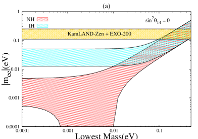
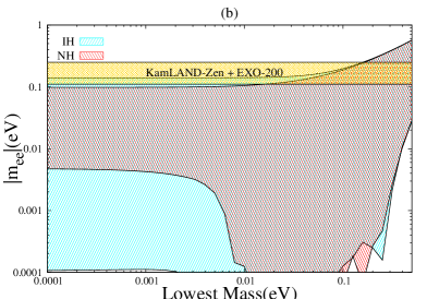
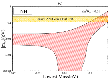
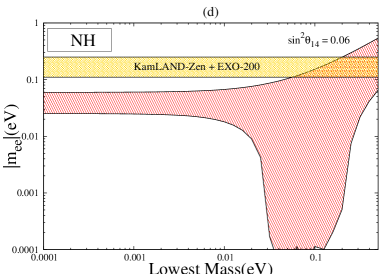
Figure 4.6: Plot of $|m_{ee}|$ versus the lowest mass. The panel (a) corresponds to the three generation case while panel (b) is for 3+1 case. In panel (b) all the mixing angles are varied in their 3$\sigma$ range and the Majorana CP violating phases are varied in their full range (0-$\pi$). The panel (c) and (d) are for specific values of $\theta_{14}$ with all other parameters covering their full range.

The modulus of $m_{ee}$ is the effective mass that can be extracted from half-life measurements in neutrinoless double beta decay. In Fig. 4.6 we plot the effective mass as a function of the smallest mass by varying $\theta_{14}$ in its complete 3$\sigma$ range as well as for specific values of the mixing angle $\theta_{14}$. The Majorana phases are varied randomly in the range 0 to $\pi$ in all the plots. The first panel is for $\theta_{14}=0$ i.e., the three generation case. It is seen that for present values of the oscillation parameters the cancellation condition is not satisfied for $m_{1}\rightarrow 0$ for NH. However, as one increases $m_{1}$, complete cancellation can be achieved. For IH the complete cancellation is never possible. These results change when we include the sterile contribution as is evident from the panel (b) in Fig. 4.6 which shows the effective mass for NH and IH by varying all the parameters in their full 3$\sigma$ allowed range. The behaviour can be understood from the expressions of $|m_{ee}|$ in various limiting cases. For NH, in the hierarchical limit of $m_{1}\rightarrow 0$ the major contributor will be the additional term due to the sterile neutrinos because of higher value of $m_{4}$. Complete cancellation is only possible for smaller values of $\theta_{14}$ so that this contribution is suppressed. The typical value of $\theta_{14}$ required for cancellation can be obtained by putting $\alpha=\beta=0$ (which would maximize the three neutrino contribution) and $\gamma=\pi/2$, as

$$\tan^{2}\theta_{14}\approx\frac{(\sqrt{\zeta}c_{13}^{2}s_{12}^{2}+s_{13}^{2})}{\sqrt{\xi}}\approx 10^{-3},$$ (4.33)

which lies outside the allowed range of $\theta_{14}$. As we increase $m_{1}$, $(m_{ee})_{3\nu}$ increases and can be of the same order of magnitude of the sterile term. Hence one can get cancellation regions. The cancellation is mainly controlled by the value of $\theta_{14}$. For higher values of $s_{14}^{2}$ one needs a higher value of $m_{1}$ for cancellation to occur. This correlation between $m_{1}$ and $\theta_{14}$ is brought out by the panels (c) and (d) in Fig. 4.6.

For IH case, in the limit of vanishing $m_{3}$ using approximation in Eq. 4.28, $m_{ee}$ in a 3+1 scenario can be written as

$$|m_{ee}|\approx|c_{14}^{2}c_{13}^{2}\sqrt{\Delta_{31}}(c_{12}^{2}+s_{12}^{2}e^{2i\alpha})+\sqrt{\Delta_{43}}s_{14}^{2}e^{2i\gamma}|.$$ (4.34)

The maximum value of this is achieved for $\alpha=\gamma=0$ which is slightly lower than that of NH in this limit. The element vanishes in the limit $m_{3}\approx$ 0 eV when $\alpha=0$ and $\gamma=\pi/2$ provided

$$\tan^{2}\theta_{14}\approx\frac{c_{13}^{2}}{\sqrt{\xi}}\approx 0.05.$$ (4.35)

This is well within the allowed range. This behaviour is in stark contrast to that in the 3 neutrino case [257] . There is no significant change in this behaviour as the smallest mass $m_{3}$ is increased since this contribution is suppressed by the $s_{13}^{2}$ term and the dominant contribution to $(m_{ee})_{3\nu}$ comes from the first two terms in Eq. 4.30. Therefore in this case we do not observe any correlation between $m_{3}$ and $s_{14}^{2}$.

While moving towards the quasi-degenerate regime of $m_{1}\approx m_{2}\approx m_{3}$ we find that effective mass can still be zero. However, when the lightest mass approaches a larger value $\sim 0.3$ eV we need very large values of active sterile mixing angle $\theta_{14}$, outside the allowed range, for cancellation. Hence the effective mass cannot vanish for such values of masses.

Also shown is the current limit on effective mass from combined KamLAND-Zen and EXO 200 results on the half-life of $0\nu\beta\beta$ in ¹³⁶Xe [258, 259]. When translated in terms of effective mass this corresponds to the bound $|m_{ee}|<0.11-0.24$ eV including nuclear matrix element uncertainties. For the three generation case, the hierarchical neutrinos cannot saturate this bound. But in the 3+1 scenario this bound can be reached even for very small values of $m_{3}$ for IH and for some parameter values it can even exceed the current limit. Thus from the present limits on neutrinoless double beta decay searches a part of the parameter space for smaller values of $m_{3}$ can be disfavoured for IH. For NH, the KamLAND-Zen + EXO 200 combined bound is reached for $m_{1}=0.02$ eV and again some part of the parameter space can be disfavoured by this bound.

4.5.2.2 The Mass Matrix Element $m_{e\mu}$

The mass matrix element $m_{e\mu}$ in the presence of extra sterile neutrino is given as

$$m_{e\mu} = c_{14}(e^{i(\delta_{14}-\delta_{24}+2\gamma)}m_{4}s_{14}s_{24}+e^{i(\delta_{13}+2\beta)}m_{3}s_{13}(c_{13}c_{24}s_{23}-e^{i(\delta_{14}-\delta_{13}-\delta_{24})}$$

$$s_{13}s_{14}s_{24})+c_{12}c_{13}m_{1}(-c_{23}c_{24}s_{12}+c_{12}(-e^{i\delta_{13}}c_{24}s_{13}s_{23}-e^{i(\delta_{14}-\delta_{24})}c_{13}s_{14}s_{24}))$$

$$+ e^{2i\alpha}m_{2}c_{13}s_{12}(c_{12}c_{23}c_{24}+s_{12}(-e^{i\delta_{13}}c_{24}s_{13}s_{23}-e^{i(\delta_{14}-\delta_{24})}c_{13}s_{14}s_{24}))).$$

Unlike $m_{ee}$ here the expression is complicated and an analytic understanding is difficult from the full expression. The expression for $m_{e\mu}$ in the limit of vanishing active sterile mixing angle $\theta_{24}$ becomes

$$m_{e\mu}=c_{14}(m_{e\mu})_{3\nu}.$$

Since the active sterile mixing is small, in order to simplify these expressions we introduce a quantity $\lambda\equiv$0.2 and define these small angles to be of the form $a\lambda$. Thus a systematic expansion in terms of $\lambda$ can be done. For sterile mixing angle

$${\mathrm{sin}}\theta_{14}\approx\theta_{14}\equiv\chi_{14}\lambda,$$

$${\mathrm{sin}}\theta_{24}\approx\theta_{24}\equiv\chi_{24}\lambda,$$ (4.37)

and the reactor mixing angle as

$$\sin\theta_{13}\approx\theta_{13}\equiv\chi_{13}\lambda.$$ (4.38)

Here $\chi_{ij}$ are parameters of $\mathcal{O}$(1) and their $3\sigma$ range from the current constraint on the mixing angles is given by

$$\chi_{13} = 0.65-0.9,$$ (4.39)

$$\chi_{14} = 0.5-1.2,$$

$$\chi_{24} = 0.25-1.$$

Note that for the sterile mixing angle $\theta_{34}$ we do not adopt the above approximation because this angle can be large compared to other two sterile mixing angles and hence the small parameter approximation will not be valid.

Using the approximation in Eqs. 4.27, 4.5.2.2 and 4.38 we get the expression for $|m_{e\mu}|$ for normal hierarchy as

$$|m_{e\mu}| \approx |\sqrt{\Delta_{32}}\{\sqrt{\zeta}s_{12}c_{12}c_{23}e^{2i\alpha}+e^{i\delta_{13}}(e^{2i\beta}-e^{2i\alpha}\sqrt{\zeta}s_{12}^{2})s_{23}\lambda\chi_{13}$$

$$+ \lambda^{2}e^{i(\delta_{14}-\delta_{24})}(e^{2i\gamma}\sqrt{\xi}-e^{2i\alpha}\sqrt{\zeta}s_{12}^{2})\chi_{14}\chi_{24}\}|.$$

To see the order of magnitude of the different terms we choose vanishing Majorana phases while Dirac CP phases are taken as $\pi$. The mass matrix element $m_{e\mu}$ vanishes when

$$\sqrt{\zeta}s_{12}c_{12}c_{23}-(1-\sqrt{\zeta}s_{12}^{2})s_{23}\lambda\chi_{13}+\lambda^{2}(\sqrt{\xi}-\sqrt{\zeta}s_{12}^{2})\chi_{14}\chi_{24}=0.\\$$ (4.41)

The three generation limit is recovered for $s_{24}^{2}=0$ and in panel (a) of Fig. 4.7 we show $|m_{e\mu}|$ as a function of $m_{1}$ of this case, for NH. Panel (b) (red/light region) of Fig. 4 shows $|m_{e\mu}|$ for the 3+1 case, with all parameters varied randomly within their $3\sigma$ range. The figures show that $|m_{e\mu}|=0$ can be achieved over the whole range of the smallest mass for both 3 and 3+1 cases. However, we find that in the hierarchical limit cancellation is not achieved for large values of $\theta_{24}$, since in that case the third term of Eq. 4.41 will be of the $\mathcal{O}$ (10^-1) compared to the leading order term which is of the $\mathcal{O}$ (10^-2) and hence there will be no cancellation of these terms. This can be seen from panel (b) (green/dark region) of Fig. 4.7 for $s_{24}^{2}=0.04$. In the QD limit the contribution from the active terms are large enough to cancel the sterile contribution and thus $|m_{e\mu}|=0$ can be achieved.

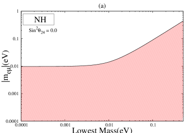
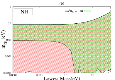
Figure 4.7: Plots of $|m_{e\mu}|$ as a function of the lowest mass $m_{1}$ for NH. Panel (a) correspond to the three generation case while (b) (red/light region) is for 3+1 case and also for $s_{24}^{2}=0.04$ (green/dark region). All the parameters are varied in their full 3$\sigma$ allowed range, the CP violating Dirac phases are varied from 0 to $2\pi$ and the Majorana phases are varied from 0 to $\pi$ unless otherwise stated.

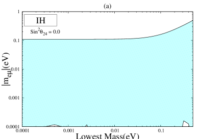
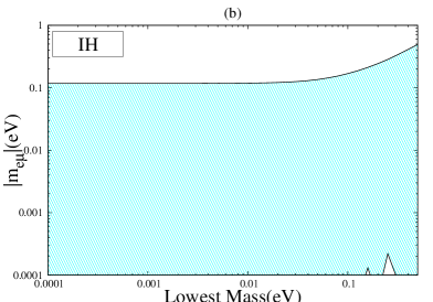
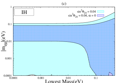
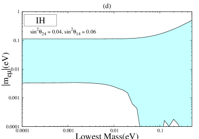
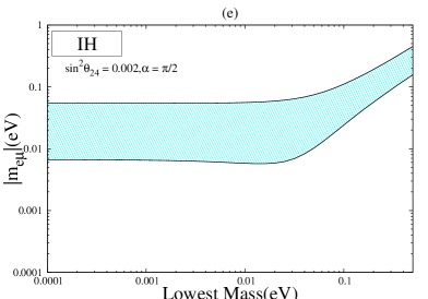
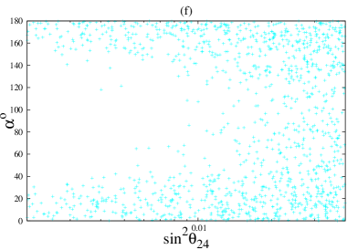
Figure 4.8: Plots of $|m_{e\mu}|$ vs $m_{3}$ for inverted hierarchy for (a) three generation case (b) 3+1 case with all parameters varied randomly in their full range. Panel (c), (d) and (e) are for specific values of $s_{24}^{2}$ and $\alpha$. The panel (f) shows the correlation between $\alpha$ and $s_{24}^{2}$ when all other parameters are randomly varied.

For IH using the approximation Eq. 4.28 for the hierarchical limit we get the expression

$$|m_{e\mu}| \approx |\sqrt{\Delta_{31}}\{c_{12}s_{12}c_{23}(e^{2i\alpha}-1)-e^{i\delta_{13}}(c_{12}^{2}+s_{12}^{2}e^{2i\alpha})s_{23}\chi_{13}\lambda$$

$$- e^{i(\delta_{14}-\delta_{24})}\lambda^{2}\chi_{14}\chi_{24}(c_{12}^{2}-e^{2i\gamma}\sqrt{\xi}+e^{2i\alpha}s_{12}^{2})\}|.$$

To see the order of magnitude of the various terms we consider the case when Majorana phases vanish and the Dirac phases assume the value $\pi$. Then we get for vanishing $m_{e\mu}$,

$$s_{23}\lambda\chi_{13}-\lambda^{2}(1-\sqrt{\xi})\chi_{14}\chi_{24}=0.$$ (4.43)

In panel (a) of Fig. 4.8 we display the plot of $|m_{e\mu}|$ with $m_{3}$ for the 3 generation scenario i.e., for $\sin^{2}\theta_{24}=0$ for IH. In panel (b) we consider the 3+1 case with all the parameters varying in their allowed range. Note that in the small $m_{3}$ limit for $\alpha=0$ the leading order term vanishes. For this case, for large active sterile mixing angle $\theta_{24}$, the $\lambda^{2}$ term becomes large $\mathcal{O}$ (10^-1) and the cancellation with $\lambda$ term is not be possible. When CP violating phase $\alpha$ is non zero, the leading order term can cancel the $\lambda^{2}$ term even for large values of $s_{24}^{2}$. These features are reflected in panel (c) where we plot $|m_{e\mu}|$ for $s_{24}^{2}=0.04$ and $\alpha=0$ (blue/dark region) and by varying $\alpha$ in its full range (cyan/light region). As expected, for $\alpha=0$, cancellation is not achieved for smaller values of $m_{3}$. Thus the condition $|m_{e\mu}|=0$ implies some correlation between $m_{3}$ and $\alpha$ for IH. Even if $\alpha$ is varied in its full range, the absolute value of the matrix element $|m_{e\mu}|$ can vanish only if the product $\chi_{14}\chi_{24}$ is small, i.e., $s_{14}^{2}$ and $s_{24}^{2}$ are simultaneously small . This is because if they are large the $\lambda^{2}$ term becomes of the $\mathcal{O}$ (10^-1) and hence cancellation will not be possible. This is seen from panel (d) where for $s_{14}^{2}=0.06$ and $s_{24}^{2}=0.04$ the region where $m_{3}$ is small gets disallowed. Taking CP violating phase $\alpha=\pi/2$ makes the magnitude of leading order term ($s_{12}c_{12}c_{23}\sqrt{\zeta}$) quite large and smaller values of $\theta_{24}$ cannot give cancellation even for large values of $m_{3}$ which can be seen from panel (e) of Fig. 4.8. For the occurrence of cancellation $s_{24}^{2}$ has to be $\geq$ 0.01 for $\alpha=\pi/2$ as can be seen from panel (f) where we have plotted the correlation between $\alpha$ and $s_{24}^{2}$ for $|m_{e\mu}|=0$.

4.5.2.3 The Mass Matrix Element $m_{e\tau}$

The mass matrix element $m_{e\tau}$ in the presence of an extra sterile neutrino is given by

$$m_{e\tau} = c_{14}c_{24}e^{i(2\gamma+\delta_{14})}m_{4}s_{14}s_{34}+m_{3}c_{14}s_{13}e^{i(2\beta+\delta_{13})}(-c_{24}s_{13}s_{14}s_{34}e^{i(\delta_{14}-\delta_{13})}$$

$$+ c_{13}(c_{23}c_{34}-e^{i\delta_{24}}s_{23}s_{24}s_{34}))+m_{2}s_{12}c_{13}c_{14}e^{2i\alpha}(c_{12}(-c_{34}s_{23}-c_{23}s_{24}s_{34}e^{i\delta_{24}})$$

$$+ s_{12}(-c_{13}c_{24}s_{14}s_{34}e^{i\delta_{14}}-e^{i\delta_{13}}s_{13}(c_{23}c_{34}-e^{i\delta_{24}}s_{23}s_{24}s_{34})))$$

$$+ m_{1}c_{12}c_{13}c_{14}(-s_{12}(-c_{34}s_{23}-c_{23}s_{24}s_{34}e^{i\delta_{24}})+c_{12}(-c_{13}c_{24}s_{14}s_{34}e^{i\delta_{14}}-e^{i\delta_{13}}s_{13}$$

$$(c_{23}c_{34}-e^{i\delta_{24}}s_{23}s_{24}s_{34}))).$$

As mentioned in the previous section, the elements $m_{e\tau}$ and $m_{e\mu}$ are related by $\mu-\tau$ permutation symmetry and it is found that in the limit of small $\theta_{24}$ the two active sterile mixing angles $\bar{\theta}_{24}\approx\theta_{34}$. (Eq. 4.17) The same can be seen from Eq. 4.19 which gives $\bar{\theta}_{34}\approx\theta_{24}$ for smaller values of the mixing angle $\theta_{34}$. Thus, for these cases the behaviour shown by $\theta_{24}$ in $m_{e\mu}$ ($m_{\mu\mu}$) is same as shown by $\theta_{34}$ in $m_{e\tau}$ ($m_{\tau\tau}$).

In the limit of vanishing active sterile mixing angle $\theta_{34}$ this element becomes

$$m_{e\tau}=c_{14}(m_{e\tau})_{3\nu}.$$

Using the approximation in Eq. 4.27 for NH the above element can be expressed as,

$$|m_{e\tau}| \approx |\sqrt{\Delta_{32}}\{-s_{12}s_{23}c_{12}c_{34}\sqrt{\zeta}e^{2i\alpha}+\lambda(c_{23}c_{34}e^{i(2\beta+\delta_{13})}\chi_{13}-c_{23}c_{34}s_{12}^{2}$$

$$\chi_{13}\sqrt{\zeta}e^{i(2\alpha+\delta_{13})}+e^{i(2\gamma+\delta_{14})}\sqrt{\xi}s_{34}\chi_{14}-e^{i(2\alpha+\delta_{14})}\sqrt{\zeta}s_{12}^{2}s_{34}\chi_{14}-c_{12}c_{23}$$

$$e^{i(2\alpha+\delta_{24})}s_{12}s_{34}\chi_{24}\sqrt{\zeta})-e^{i(\delta_{13}+\delta_{24})}(e^{2i\beta}-e^{2i\alpha}s_{12}^{2}\sqrt{\zeta})s_{23}s_{34}\chi_{13}\chi_{24}\lambda^{2}\}|.$$

For the case of vanishing Majorana phases and Dirac phases having the value $\pi$, this element can vanish when

$$- c_{12}c_{34}\sqrt{\zeta}s_{12}s_{23}-(1-\sqrt{\zeta}s_{12}^{2})s_{23}s_{34}\lambda^{2}\chi_{13}\chi_{24}+\lambda(-c_{23}c_{34}\chi_{13}+$$

$$\sqrt{\zeta}c_{23}s_{12}(c_{34}s_{12}\chi_{13}+c_{12}s_{34}\chi_{24})+s_{12}^{2}s_{34}\chi_{14}\sqrt{\zeta}-\sqrt{\xi}s_{34}\chi_{14})=0.$$

For a vanishing active sterile mixing angle $\theta_{34}$ one recovers the 3 generation case. In this limit, from Eq. 4.5.2.3 one observes that the leading order term and the term with $\lambda$ are of the same order $\sim\mathcal{O}$ (10^-2) while the $\lambda^{2}$ term vanishes and hence cancellation is possible excepting for very low values of the lightest mass. We can see this in panel (a) of Fig. 4.9. In panel (b) (red/light region) all the parameters are varied randomly (3+1 case) and cancellation is seen to be possible over the whole range of $m_{1}$.

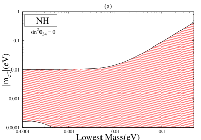
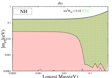
Figure 4.9: Plots of $|m_{e\tau}|$ for normal hierarchy with lowest mass $m_{1}$. The panel (a) corresponds to three generation case. In (b) (red/light region) all the parameters are varied in their full allowed range and the green/dark region is for $s_{34}^{2}=0.18$ with all the other parameters covering their full range.

In panel (b) (green/dark region) we also plot the element $|m_{e\tau}|$ for the upper limit of $s_{34}^{2}=0.18$. In this case there is no cancellation for very low values of the smallest mass. This is because when $s_{34}^{2}$ is large, the $\lambda$ term containing $\xi$ becomes large $\mathcal{O}$ (1) and there will be no cancellation.
For inverted hierarchy the element $m_{e\tau}$ using the approximation in Eq. 4.28 becomes

$$|m_{e\tau}| \approx |\sqrt{\Delta_{31}}\{c_{12}c_{34}s_{12}s_{23}(-e^{2i\alpha}+1)+e^{i(\delta_{13}+\delta_{24})}(c_{12}^{2}+e^{2i\alpha}s_{12}^{2})s_{23}s_{34}\lambda^{2}\chi_{13}\chi_{24}$$ (4.47)

$$- \lambda(c_{23}c_{34}\chi_{13}e^{i\delta_{13}}(c_{12}^{2}+e^{2i\alpha}s_{12}^{2})+e^{i\delta_{14}}s_{34}\chi_{14}(c_{12}^{2}+e^{i\alpha}s_{12}^{2})$$

$$- e^{i(2\gamma+\delta_{14})}s_{34}\chi_{14}\sqrt{\xi}+c_{12}c_{23}s_{12}s_{34}\chi_{24}e^{i\delta_{24}}(e^{2i\alpha}-1))\}|$$

In the limit of vanishing Majorana phases and Dirac CP violating phases equal to $\pi$ this element becomes negligible when

$$\lambda(c_{23}c_{34}\chi_{13}+s_{34}\chi_{14}-s_{34}\chi_{14}\sqrt{\xi})+s_{23}s_{34}\chi_{13}\chi_{24}\lambda^{2}=0.$$ (4.48)

In panel (a) of Fig. 4.10 the three generation case is reproduced by putting $s_{34}^{2}=0$ and in (b) all the parameters are varied in their allowed range (3+1 case). In both the figures we can see that cancellation is permissible over the whole range of $m_{3}$ considered. When the CP violating phase $\alpha=0$ we see that the leading order term ($\sin 2\theta_{12}s_{23}c_{34}$) vanishes and as a result for large values of $s_{34}^{2}$ the cancellation is not possible because the term with coefficient $\lambda$ becomes large ($\mathcal{O}$(10^-1)). For non zero values of the CP violating phase $\alpha$ this leading order term is non zero and its contribution will be significant. So in this case high values of $\theta_{34}$ are also allowed because now the leading order and the term with coefficient $\lambda$ will be of same magnitude. When we fix $s_{34}^{2}=0.06$ and $\alpha=0$ the region where $m_{3}$ is small is disallowed (panel (c) blue/dark region) but when $\alpha$ varies within its full range the disallowed regions become allowed (panel (c) cyan/light region). When $s_{34}^{2}$ approaches its upper limit, the $\lambda$ term having $\xi$ becomes very large and cancellation is not possible even for non zero values of $\alpha$ which can be seen from panel (d). However, when $\alpha=\pi/2$, very small values of $s_{34}^{2}$ cannot give cancellation as the leading order term becomes large (panel (e)). $s_{34}^{2}$ has to be $\geq$ 0.01 for the term to vanish which can be seen from panel (f) where we plotted the correlation between $\alpha$ and $s_{34}^{2}$ for $|m_{e\tau}|=0$.

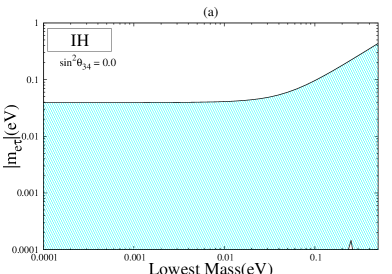
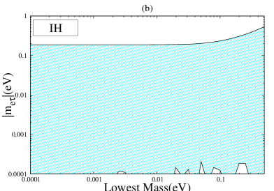
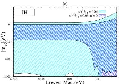
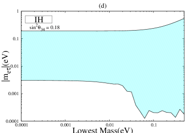
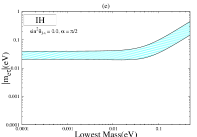
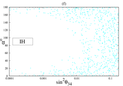
Figure 4.10: Plots of $|m_{e\tau}|$ for inverted hierarchy with lowest mass $m_{3}$. The panel (a) corresponds to three generation case. In (b) all the parameters are varied in their full allowed range (3+1). The panel (c), (d) is for specific value of $\theta_{34}$ and $\alpha$ with all the other parameters covering their full range. The panel (f) shows correlation between $\alpha$ and $s_{24}^{2}$.

4.5.2.4 The Mass Matrix Element $m_{\mu\mu}$

The (2,2) diagonal entry in neutrino mass matrix is given as

$$m_{\mu\mu} = e^{2i(\delta_{14}-\delta_{24}+\gamma)}c_{14}^{2}m_{4}s_{24}^{2}$$

$$+ e^{2i(\delta_{13}+\beta)}m_{3}(c_{13}c_{24}s_{23}-e^{i(\delta_{14}-\delta_{13}-\delta_{24})}s_{13}s_{14}s_{24})^{2}$$

$$+ m_{1}\{-c_{23}c_{24}s_{12}+c_{12}(-e^{i\delta_{13}}c_{24}s_{13}s_{23}-e^{i(\delta_{14}-\delta_{24})}c_{13}s_{14}s_{24})\}^{2}$$

$$+ e^{2i\alpha}m_{2}\left\{c_{12}c_{23}c_{24}+s_{12}(-e^{i\delta_{13}}c_{24}s_{13}s_{23}-e^{i(\delta_{14}-\delta_{24})}c_{13}s_{14}s_{24})\right\}^{2}$$

This expression reduces to its three generation case if the mixing angle $\theta_{24}$ vanishes. Also we can see from the expression that there is no dependence on the mixing angle $\theta_{34}$. Using the approximation in Eqs. 4.27 this element can be simplified to the form

$$|m_{\mu\mu}| \approx |\sqrt{\Delta_{32}}\{c_{12}^{2}c_{23}^{2}e^{2i\alpha}\sqrt{\zeta}+e^{i(\delta_{13}+2\beta)}s_{23}^{2}$$

$$- 2\lambda c_{12}c_{23}e^{i(\delta_{13}+2\alpha)}\sqrt{\zeta}s_{12}s_{23}\chi_{13}$$

$$+ \lambda^{2}\{e^{2i(\delta_{13}+\alpha)}\sqrt{\zeta}s_{12}^{2}s_{23}^{2}\chi^{2}_{13}+e^{i(\delta_{14}-\delta_{24})}(e^{i(2\gamma+\delta_{14}-\delta_{24})}\sqrt{\xi}\chi_{24}$$

$$- 2e^{2i\alpha}\sqrt{\zeta}c_{12}c_{23}s_{12}\chi_{14})\chi_{24}\}\}|.$$

For the case of Majorana CP phases having the value 0 and the Dirac phases having the value $\pi$, this element vanishes when

$$s_{23}^{2}+c_{12}^{2}c_{23}^{2}\sqrt{\zeta}+c_{12}s_{12}\sin 2\theta_{23}\sqrt{\zeta}\lambda\chi_{13}$$

$$+ \lambda^{2}(s_{12}^{2}s_{23}^{2}\sqrt{\zeta}\chi_{13}^{2}-c_{23}\sin 2\theta_{12}\sqrt{\zeta}\chi_{14}\chi_{24}+\sqrt{\xi}\chi_{24}^{2})=0.$$

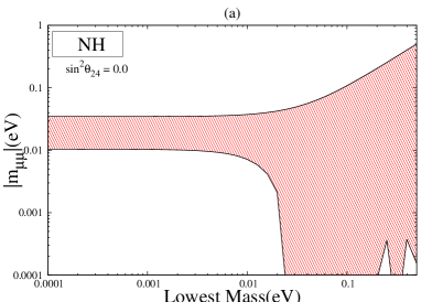
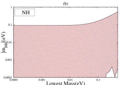
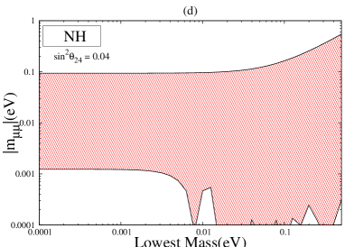
Figure 4.11: Plots of vanishing $m_{\mu\mu}$ for normal hierarchy for different values of $\theta_{24}$ when all other mixing angles are varied in their 3$\sigma$ ranges, Dirac CP phases are varied from 0 to $2\pi$ and Majorana phases from 0 to $\pi$.

We know that for the case of 3 generations, the elements in the $\mu-\tau$ block are quite large and cannot vanish for normal hierarchy. In panel (a) of Fig. 4.11 we can see that $|m_{\mu\mu}|$ cannot vanish in small $m_{1}$ region for $s_{24}^{2}=0$ which is indeed the 3 generation case. This is because the magnitude of the first two terms in Eq. 4.5.2.4 is quite large in this case, $\sim\mathcal{O}$ (10^-1) and for cancellation to occur the term with coefficient $\lambda^{2}$ has to be of the same order. This is not possible when $s_{24}^{2}$ is small. However when $s_{24}^{2}$ is varied in its full allowed range the contribution of the sterile part is enhanced and this can cancel the active part as can be seen from panel (b). Now to understand the dependence of $m_{\mu\mu}$ with $\theta_{24}$ we note that if we increase $s_{24}^{2}$ from its lower bound then the two terms become of the same order. So there will be regions in the limit of small $m_{1}$ for which this element vanishes (panel (c)). We see in panel (d) of Fig. 4.11 that when $\theta_{24}$ acquires very large values, the magnitude of the $\lambda^{2}$ ($\sqrt{\xi}\chi_{24}^{2}$) term becomes large, thus leading to non cancellation of the terms with the leading order first two terms. Hence, the region with very small $m_{1}$ is not allowed. Using the approximation for inverted hierarchy the element $m_{\mu\mu}$ becomes

$$|m_{\mu\mu}| \approx |\sqrt{\Delta_{31}}\{c_{23}^{2}(s_{12}^{2}+c_{12}^{2}e^{2i\alpha})$$

$$+ \frac{1}{2}\lambda\sin 2\theta_{12}\sin 2\theta_{23}e^{i\delta_{13}}(1-e^{2i\alpha})\chi_{13}$$

$$+ \lambda^{2}[\sin 2\theta_{12}c_{23}e^{i(\delta_{14}-\delta_{24})}(1-e^{2i\alpha})\chi_{14}\chi_{24}+s_{23}^{2}e^{2i\delta_{13}}(c_{12}^{2}+e^{2i\alpha}s_{12}^{2})\chi_{13}^{2}$$

$$+ e^{2i(\gamma+\delta_{14}-\delta_{24})}\sqrt{\xi}\chi_{24}^{2}]\}|.$$

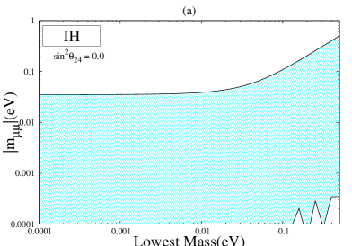
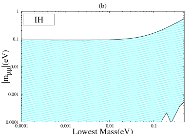
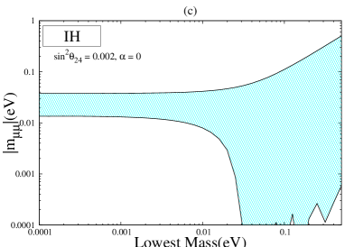
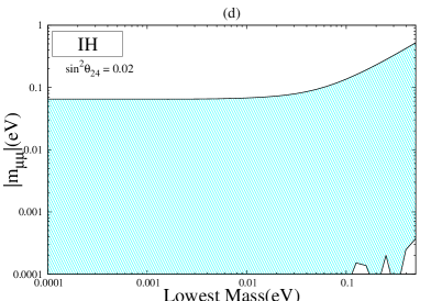
Figure 4.12: Plots of vanishing $m_{\mu\mu}$ for inverted hierarchy with lowest mass $m_{3}$. Panel (a) for 3 generation case (b) all the parameters are varied in full allowed range (3+1). Panel (c) and (d) are for specific values of $\alpha$ and $s_{24}^{2}$ are taken with all other parameters covering their full range.

Assuming Majorana phases to be zero and Dirac phases having value $\pi$, this element can vanish when

$$c_{23}^{2}+\lambda^{2}(s_{23}^{2}\chi_{13}^{2}+\sqrt{\xi}\chi_{24}^{2})=0.$$ (4.53)

In panel (a) of Fig. 4.12 we plotted $|m_{\mu\mu}|$ for $s_{24}^{2}=0$ to reproduce 3 generation case whereas in panel (b) all the parameters are varied in their allowed range in 3+1 scenario. In both cases we can see that cancellation is possible for full range of $m_{3}$. It can be noticed that unlike normal hierarchy, here cancellation is possible for small values of $s_{24}^{2}$ because in this case all the terms are of same order and there can always be cancellations. However, if we put $\alpha=0$ then the term $\lambda$ ($\sin 2\theta_{12}s_{23}c_{23}\chi_{13}$) drops out from the equation and the leading order term can not be canceled for small values of $s_{24}^{2}$. It can be seen from panel (c) that for $s_{24}^{2}=0.002$ and $\alpha=0$ the regions where $m_{3}$ is small is not allowed. As the value of $\theta_{24}$ increases there is the possibility of cancellation of terms for all the values of $\alpha$ as can be seen from panel (d) where we plot $|m_{\mu\mu}|$ with the lowest mass for $s_{24}^{2}=0.02$ when all the other mixing angles are varied in 3$\sigma$ range and CP violating phases are varied in full range. Now if we keep increasing $s_{24}^{2}$ then $\lambda^{2}$ term will become large and the chance of cancellation will be less.

4.5.2.5 The Mass Matrix Element $m_{\mu\tau}$

The (2,3) element of $M_{\nu}$ in the flavor basis becomes quite complicated in the presence of an extra sterile neutrino. The expression is

$$m_{\mu\tau} = e^{i(2\delta_{14}-\delta_{24}+2\gamma)}c_{14}^{2}c_{24}m_{4}s_{24}s_{34}$$

$$+ e^{2i(\delta_{13}+\beta)}m_{3}(c_{13}c_{24}s_{23}-e^{i(\delta_{14}-\delta_{24}-\delta_{13})}s_{13}s_{14}s_{24})$$

$$\{-e^{i(\delta_{14}-\delta_{13})}c_{24}s_{13}s_{14}s_{34}+c_{13}(c_{23}c_{34}-e^{i\delta_{24}}s_{23}s_{24}s_{34})\}$$

$$+ m_{1}\{-c_{23}c_{24}s_{12}+c_{12}(-e^{i\delta_{13}}c_{24}s_{13}s_{23}-e^{i(\delta_{14}-\delta_{24})}c_{13}s_{14}s_{24})\}$$

$$[-s_{12}(-c_{34}s_{23}-e^{i\delta_{24}}c_{23}s_{24}s_{34})$$

$$+ c_{12}\{-e^{i\delta_{14}}c_{13}c_{24}s_{14}s_{34}-e^{i\delta_{13}}s_{13}(c_{23}c_{34}-e^{i\delta_{24}}s_{23}s_{24}s_{34})\}]$$

$$+ e^{2i\alpha}m_{2}\{c_{12}c_{23}c_{24}+s_{12}(-e^{i\delta_{13}}c_{24}s_{13}s_{23}-e^{i(\delta_{14}-\delta_{24})}c_{13}s_{14}s_{24})\}$$

$$[c_{12}(-c_{34}s_{23}-e^{i\delta_{24}}c_{23}s_{24}s_{34})$$

$$+ s_{12}\{-e^{i\delta_{14}}c_{13}c_{24}s_{14}s_{34}-e^{i\delta_{13}}s_{13}(c_{23}c_{34}-e^{i\delta_{24}}s_{23}s_{24}s_{34})\}].$$

It reduces to the 3 generation case when $\theta_{24}=\theta_{34}=0$. In the normal hierarchical region where $m_{1}$ can assume very small values and can be neglected, using approximations in Eqs. 4.27, 4.5.2.2 and 4.38 we get

$$|m_{\mu\tau}| \approx |\sqrt{\Delta_{32}}\{c_{23}c_{34}(e^{2i(\beta+\delta_{13})}-e^{2i\alpha}\sqrt{\zeta}c_{12}^{2})s_{23}$$

$$- \lambda[c_{12}c_{34}e^{i(2\alpha+\delta_{13})}\sqrt{\zeta}s_{12}\cos 2\theta_{23}\chi_{13}+e^{i\delta_{24}}(e^{2i\alpha}c_{12}^{2}c_{23}^{2}\sqrt{\zeta}+e^{2i(\beta+\delta_{13})}s_{23}^{2})\chi_{24}s_{34}$$

$$- e^{2i\delta_{14}}(e^{i(2\gamma-\delta_{24})}\sqrt{\xi}\chi_{24}-c_{12}c_{23}e^{2i\alpha}\sqrt{\zeta}s_{12}\chi_{14})s_{34}]$$

$$+ \lambda^{2}[\sqrt{\zeta}e^{i(2\alpha+\delta_{13})}(e^{i\delta_{14}}s_{12}\chi_{14}+2c_{12}c_{23}e^{i\delta_{24}}\chi_{24})s_{12}s_{23}s_{34}\chi_{13}$$

$$+ e^{i\delta_{14}}(e^{i(2\alpha-\delta_{24})}c_{12}c_{34}\sqrt{\zeta}s_{12}\chi_{24}-e^{i(2\beta+\delta_{13})}\chi_{13}s_{34})\chi_{14}s_{23}$$

$$+ c_{23}c_{34}e^{2i(\alpha+\delta_{13})}s_{12}^{2}\chi_{13}^{2}\sqrt{\zeta}s_{23}]\}|.$$

To see the order of the terms we consider the case where Majorana CP phases vanish and Dirac phases have the value $\pi$. In this limit the element becomes negligible when

$$c_{23}c_{34}s_{23}(1-c_{12}^{2}\sqrt{\zeta})+\lambda\{(c_{12}c_{34}s_{12}\sqrt{\zeta}\chi_{13})\cos 2\theta_{23}$$

$$+ \chi_{24}s_{34}(s_{23}^{2}+c_{12}^{2}c_{23}^{2}\sqrt{\zeta})+s_{34}(\sqrt{\xi}\chi_{24}+c_{12}c_{23}s_{12}\sqrt{\zeta}\chi_{14})\}$$

$$+ \lambda^{2}\{s_{12}\chi_{13}s_{23}s_{34}\sqrt{\zeta}(s_{12}\chi_{14}+2c_{12}c_{23}\chi_{24})+\chi_{14}s_{23}(c_{12}c_{34}s_{12}^{2}s_{23}\sqrt{\zeta}\chi_{13}^{2})\}=0.$$

Being an element of $\mu\tau$ block, $m_{\mu\tau}$ shows the same behaviour that of $m_{\mu\mu}$ in normal hierarchy. In panel (a) of Fig. 4.13 we plotted $|m_{\mu\tau}|$ for $s_{24}^{2}=s_{34}^{2}=0$ which coincides with the 3 generation case and we can see that cancellation is not possible in hierarchical region. However, when all the parameters are varied in their allowed range in panel (b) it get contribution from the sterile part and cancellation is always possible. It can also be seen from panel (c) of Fig. 4.13 that for $s_{34}^{2}=0$ there is no cancellation in the region when $m_{1}$ is small and the figure is quite similar to that of 3 generation case. However, as this active sterile mixing angle becomes larger there is always a possibility of allowed region towards the lower values of $m_{1}$ as is evident from panel (d). This is because for the vanishing value of $\theta_{34}$ the terms with $\lambda$ and $\lambda^{2}$ become very small and cannot cancel the leading term $\mathcal{O}$ (10^-1). It can also be seen that in this case (i.e., $s_{34}^{2}=0$), there is no $\chi_{24}$ term and this is why the figure is somewhat similar to the 3 generation case. However, when $\theta_{34}$ increases these two contributions become large and cancellation becomes possible.

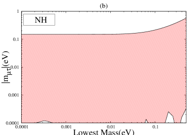
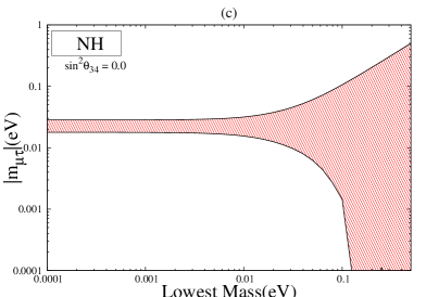
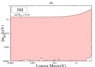
Figure 4.13: Plots of vanishing $m_{\mu\tau}$ for normal hierarchy (a) for vanishing $\theta_{34}$ and $\theta_{24}$. In panel (b) all parameters are varied in their full allowed range. Panel(c, d) are for specific values of $\theta_{34}$ when all other mixing angles are varied in their full range.

For the case of inverted hierarchy where $m_{3}$ can have very small values, $m_{\mu\tau}$ becomes

$$|m_{\mu\tau}| \approx |\sqrt{\Delta_{31}}\{-c_{23}c_{34}s_{23}(c_{12}^{2}e^{2i\alpha}+s_{12}^{2})$$

$$+ \lambda[c_{12}s_{12}(1-e^{2i\alpha})(c_{34}\cos 2\theta_{23}e^{i\delta_{13}}\chi_{13}+c_{23}s_{34}e^{i\delta_{14}}\chi_{14})$$

$$+ s_{34}\{e^{i(2\gamma+2\delta_{14}-\delta_{24})}\sqrt{\xi}-c_{23}^{2}e^{i\delta_{24}}(s_{12}^{2}+c_{12}^{2}e^{2i\alpha})\}\chi_{24}]$$

$$+ \lambda^{2}[c_{23}c_{34}s_{23}e^{2i\delta_{13}}(c_{12}^{2}+e^{2i\alpha}s_{12}^{2})\chi_{13}^{2}$$

$$+ c_{12}s_{12}s_{23}(e^{2i\alpha}-1)(c_{34}e^{i(\delta_{14}-\delta_{24})}\chi_{14}+2s_{34}c_{23}e^{i(\delta_{13}+\delta_{24})}\chi_{13})\chi_{24}]\}|.$$

To get an idea about the magnitude of the terms we take vanishing Majorana phases and Dirac CP phases to be of the order $\pi$. The expression in this case for vanishing $m_{\mu\tau}$ becomes

$$-c_{23}c_{34}s_{23}+\lambda(s_{34}\chi_{24}(c_{23}^{2}-\sqrt{\xi}))$$

$$- \lambda^{2}(-s_{34}\chi_{13}\chi_{14}-c_{23}c_{34}\chi_{13}^{2})=0$$

In panel (a) of Fig. 4.14, where $|m_{\mu\tau}|$ for 3 generation is plotted, we can see that unlike $m_{\mu\mu}$ there is no cancellation in small $m_{3}$ region but when plotted for the full range it gets contribution from the sterile part and there is cancellation for the full range of $m_{3}$ (panel (b)). Clearly the cancellation of the terms do not become possible for small values of $\theta_{34}$ in strict hierarchical region. This case is similar to the three generation case in IH (cyan/light region, panel (c)). This is because for $s_{34}^{2}=0$ the contribution of $s_{24}^{2}$ comes from the $\lambda^{2}$ term. If we put the CP violating phase $\alpha$ as zero then cancellation is not possible for whole range of $m_{3}$ (blue/dark region panel (c)). However, as the value of $s_{34}^{2}$ increases all the terms in the above equation becomes of the same order and cancellation for very small values of $m_{3}$ is possible (panel (d)).

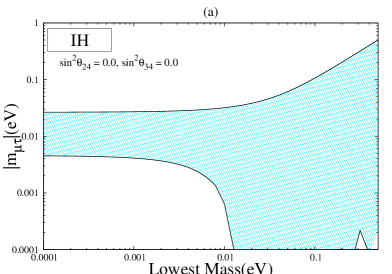
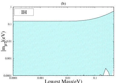
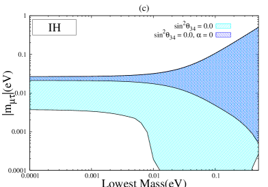
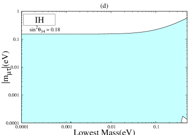
Figure 4.14: Plots of vanishing $m_{\mu\tau}$ for inverted hierarchy (a) for vanishing $\theta_{34}$ and $\theta_{24}$ (3 generation). In panel (b) all parameters are varied in their full allowed range (3+1). Panel (c) and (d) are for specific values of $\theta_{34}$ and $\alpha$ when all other mixing angles are varied in their full range.

4.5.2.6 The Mass Matrix Element $m_{\tau\tau}$

This element is related to $m_{\mu\mu}$ by the $\mu-\tau$ symmetry. As discussed earlier, in the limit when $\theta_{24}$ and $\theta_{34}$ are not very large, the two mixing angles $\theta_{34}$ and $\theta_{24}$ will behave in the same way in the textures related by $\mu-\tau$ symmetry. The (3,3) element of the neutrino mass matrix in the presence of one sterile neutrino is given as

$$m_{\tau\tau} = e^{2i(\delta_{14}+\gamma)}c_{14}^{2}c_{24}^{2}m_{4}s_{34}^{2}$$

$$+ e^{2i(\delta_{13}+\beta)}m_{3}\{e^{i(\delta_{14}-\delta_{13})}c_{24}s_{13}s_{14}s_{34}+c_{13}(c_{23}c_{34}-e^{i\delta_{24}}s_{23}s_{24}s_{34})\}^{2}$$

$$+ m_{1}[-s_{12}(-c_{34}s_{23}-e^{i\delta_{24}}c_{23}s_{24}s_{34})$$

$$+ c_{12}\{-e^{i\delta_{14}}c_{13}c_{24}s_{14}s_{34}-e^{i\delta_{13}}s_{13}(c_{23}c_{34}-e^{i\delta_{24}}s_{23}s_{24}s_{34})\}]^{2}$$

$$+ e^{2i\alpha}m_{2}[c_{12}(-c_{34}s_{23}-e^{i\delta_{24}}c_{23}s_{24}s_{34})$$

$$+ s_{12}\{-e^{i\delta_{14}}c_{13}c_{24}s_{14}s_{34}-e^{i\delta_{13}}s_{13}(c_{23}c_{34}-e^{i\delta_{24}}s_{23}s_{24}s_{34})\}]^{2}.$$

It reduces to the 3 generation case for $\theta_{34}=0$. Using the approximation for normal hierarchy in Eqs. 4.27, 4.5.2.2 and 4.38 this becomes

$$|m_{\tau\tau}| \approx |\sqrt{\Delta_{32}}\{c_{23}c_{34}s_{23}(e^{2i\beta+\delta_{13}}-c_{12}^{2}\sqrt{\zeta}e^{2i\alpha})+\lambda\{-e^{i(2\alpha+\delta_{13})}\sqrt{\zeta}$$

$$s_{12}c_{12}c_{34}\cos 2\theta_{23}\chi_{13}-\sqrt{\zeta}c_{12}c_{23}s_{34}e^{2i\alpha}(s_{12}\chi_{14}e^{i\delta_{14}}+c_{12}c_{23}\chi_{24}e^{2i\delta_{24}})$$

$$+ s_{34}\chi_{24}(-s_{23}^{2}e^{2i(\beta+\delta_{13})+i\delta_{24}}$$

$$- \sqrt{\xi}e^{2i(\gamma+\delta_{14})-i\delta_{24}})\}+\lambda^{2}\{\sqrt{\zeta}s_{12}^{2}s_{23}\chi_{13}e^{i(2\alpha+\delta_{13})}(c_{23}c_{34}\chi_{13}e^{i\delta_{13}}+s_{34}\chi_{14}e^{i\delta_{14}})$$

$$+ \sqrt{\zeta}c_{12}s_{12}s_{23}\chi_{24}e^{2i\alpha}(2c_{23}s_{34}\chi_{13}e^{i(\delta_{13}+\delta_{24})}+c_{34}\chi_{14}e^{i(\delta_{14}-\delta_{24})})$$

$$- s_{23}s_{34}\chi_{13}\chi_{14}e^{i(2\beta+\delta_{13}+\delta_{14})}\}\}|.$$

To get an idea of the order of the terms we consider the vanishing Majorana phases and the Dirac phases having the value equal to $\pi$. This element vanishes when

$$c_{23}c_{34}s_{23}(1-c_{12}^{2}\sqrt{\zeta})+$$

$$\lambda\{\sqrt{\zeta}s_{12}c_{12}c_{34}\cos 2\theta_{23}\chi_{13}+\sqrt{\zeta}c_{12}c_{23}s_{34}(s_{12}\chi_{14}$$

$$+ c_{12}c_{23}\chi_{24})-s_{34}\chi_{24}(s_{23}^{2}-\sqrt{\xi})\}+\lambda^{2}\{\sqrt{\zeta}s_{12}^{2}s_{23}\chi_{13}(c_{23}c_{34}\chi_{13}+s_{34}\chi_{14})$$

$$+ \sqrt{\zeta}c_{12}s_{12}s_{23}\chi_{24}(2c_{23}s_{34}\chi_{13}+c_{34}\chi_{14})+s_{23}s_{34}\chi_{13}\chi_{14}\}=0.$$

For vanishing $\theta_{34}$, which is the case for 3 generation, $m_{\tau\tau}=0$ is disallowed for small $m_{1}$ as can be seen from panel (a) of Fig. 4.15.

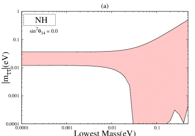
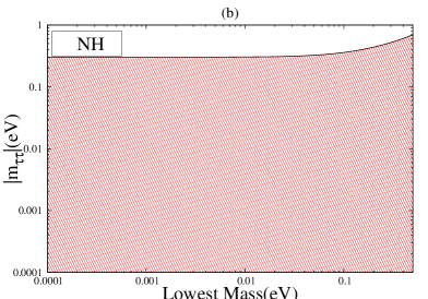
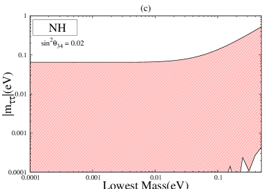
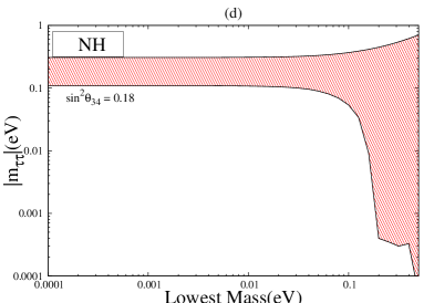
Figure 4.15: Plots of vanishing $m_{\tau\tau}$ for normal hierarchy with lowest mass $m_{1}$. Panel (a) correspond to three generation case. In panel (b) all the mixing angles are varied in their full allowed range of parameters (3+1). Panel (c) and (d) are for some specific values of $\theta_{34}$.

This is the generic behaviour of a element belonging to the $\mu-\tau$ block in normal hierarchy which we mentioned previously. This is because for $\theta_{34}$ equal to zero the leading order term is large ($\mathcal{O}$ (10^-1)). Here the term with $\lambda^{2}$ is quite small (10^-3-10^-4) and hence will not have very significant role to play. Thus, only terms with coefficient $\lambda$ can cancel the leading order term. However, for vanishing $\theta_{34}$ this term is small $\mathcal{O}$ (10^-3), and cannot cancel the leading order term. In panel (b) when all the parameters are varied in their $3\sigma$ range we can see that cancellation is possible over the whole range of $m_{1}$ (3+1 case). Now, when $\theta_{34}$ starts increasing from its lowest value there exist a region for intermediate values where both the terms become approximately of the same order and hence there can be cancellations (panel (c)). Towards very large values of $\theta_{34}$ the term with coefficient $\lambda$ becomes larger than the leading order term due to which this element cannot vanish. For the cancellation very large values of $m_{1}$ is required as can be seen from panel (d) of Fig 4.15.

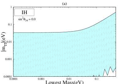
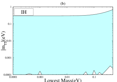
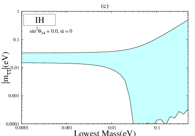
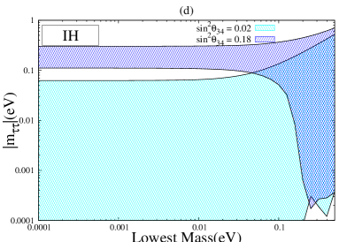
Figure 4.16: Plots of vanishing $m_{\tau\tau}$ for inverted hierarchy with lowest mass $m_{3}$. Panel (a) correspond to three generation case. In panel (b) all the mixing angles are varied in their full allowed range of parameters (3+1). Panel (c) and (d) are for some specific values of $\theta_{34}$ and $\alpha$.

For the case of inverted hierarchy where $m_{3}$ approaches small values we get the expression

$$m_{\tau\tau} \approx c_{34}^{2}s_{23}^{2}(c_{12}^{2}e^{2i\alpha}+s_{12}^{2})+e^{2i(\delta_{14}+\gamma)}\sqrt{\xi}s_{34}^{2}$$

$$+ 2\lambda[(e^{2i\alpha}-1)c_{12}c_{34}s_{12}s_{23}(c_{23}c_{34}s_{12}s_{23}(c_{23}c_{34}e^{2i\delta_{13}}\chi_{13}+e^{2i\delta_{14}}s_{34}\chi_{14})$$

$$+ 2c_{23}c_{34}e^{2i\delta_{24}}s_{23}s_{34}(c_{12}^{2}e^{2i\alpha}+s_{12}^{2})\chi_{24}]$$

$$+ \lambda^{2}[(c_{12}^{2}+e^{2i\alpha}s_{12}^{2})\{c_{23}c_{34}\chi_{13}e^{i\delta_{13}}(c_{23}c_{34}\chi_{13}e^{i\delta_{13}}+2\chi_{14}s_{34}e^{i\delta_{14}})+e^{2i\delta_{14}}\chi_{14}^{2}s_{34}^{2}\}$$

$$+ (c_{12}^{2}e^{2i\alpha}+s_{12}^{2})c_{23}^{2}e^{2i\delta_{24}}\chi_{24}^{2}s_{34}^{2}$$

$$+ 2s_{12}(e^{2i\alpha}-1)e^{i\delta_{24}}(c_{34}\chi_{13}\cos 2\theta_{23}e^{i\delta_{13}}+c_{12}c_{23}\chi_{14}s_{34})s_{34}\chi_{24}].$$

For vanishing Majorana CP phases and Dirac phases having the value equal to $\pi$ this expression becomes

$$m_{\tau\tau} \approx -c_{23}c_{34}s_{23}+\lambda s_{34}\chi_{24}(c_{23}^{2}-\sqrt{\xi})$$

$$+ \lambda^{2}s_{23}\chi_{13}(c_{23}c_{34}\chi_{13}+s_{34}\chi_{14})$$

In panel (a) of Fig. 4.16 we reproduced the 3 generation behaviour by plotting $|m_{\tau\tau}|$ for $s_{34}^{2}=0$ and in panel (b) all the parameters are varied randomly (3+1). In both the cases we can see that cancellations are possible for the whole range of $m_{3}$. For $s_{34}^{2}=0$ all the terms are of same order and cancellations are always possible. But if we put $\alpha=0$ then one term with coefficient $\lambda$ and another term with coefficient $\lambda^{2}$ drops out from the equation and then small values of $s_{34}^{2}$ can not cancel the leading order term any more. This can be seen from panel (c) where cancellation is not possible for lower $m_{3}$ region. However when $s_{34}^{2}$ increases to a value of about 0.02 this element can vanish (panel (d) the cyan region). We see that when $\theta_{34}$ increase towards its upper bound the $\lambda$ term becomes large $\mathcal{O}(1)$. Hence, the other terms are not able to cancel this term and we do not get small $m_{3}$ region allowed (Panel (d), blue region).

4.5.2.7 The Mass Matrix Elements $m_{es}$, $m_{\mu s}$, $m_{\tau s}$ and $m_{ss}$

The elements $m_{es}$, $m_{\mu s}$, $m_{\tau s}$ and $m_{ss}$ are present in the fourth row and fourth column in the neutrino mass matrix. They are the new elements that arises in 3+1 scenario due to the addition of one light sterile neutrino. The expressions for $m_{es}$, $m_{\mu s}$ and $m_{\tau s}$ are given by

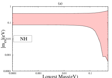
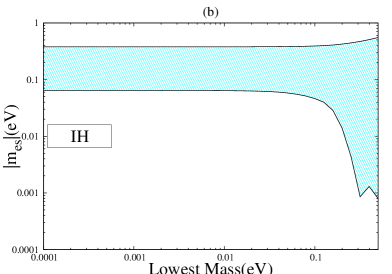
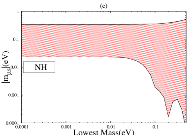
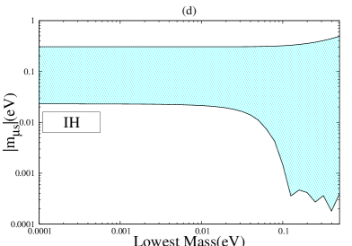
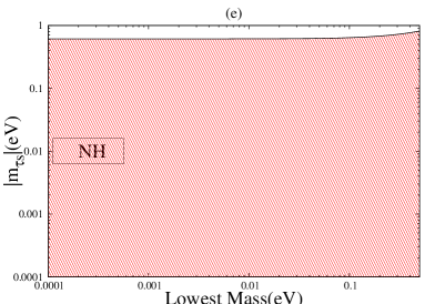
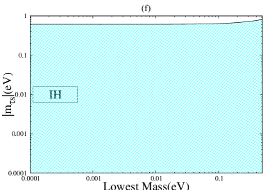
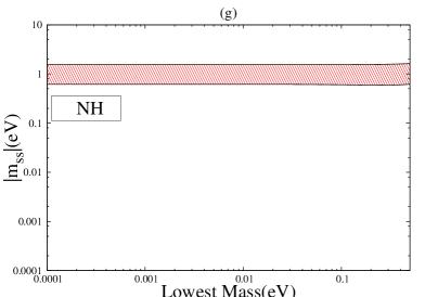
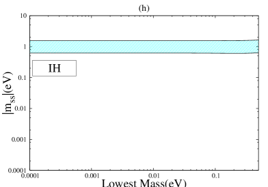
Figure 4.17: Correlation plots for vanishing $|m_{ks}|$ for both normal and inverted hierarchy. In these plots all the mixing angles are varied in their 3 $\sigma$ allowed range, Dirac CP phases are varied from 0 to $2\pi$ and Majorana phases from 0 to $\pi$.

$$m_{es} = e^{i(2\gamma+\delta_{14})}c_{14}c_{24}c_{34}m_{4}s_{14}$$

$$+ e^{i(2\beta+\delta_{13})}c_{14}m_{3}s_{13}\{-e^{i(\delta_{14}-\delta_{13})}c_{24}c_{34}s_{13}s_{14}+c_{13}(-e^{i\delta_{14}}c_{34}s_{23}s_{24}-c_{23}s_{34})\}$$

$$+ c_{12}c_{13}c_{14}m_{1}[-s_{12}(-e^{i\delta_{24}}c_{23}c_{34}s_{24}+s_{23}s_{34})$$

$$+ c_{12}\{-e^{i\delta_{14}}c_{13}c_{24}c_{34}s_{14}-e^{i\delta_{13}}s_{13}(-e^{i\delta_{24}}c_{34}s_{23}s_{24}-c_{23}s_{34})\}]$$

$$+ e^{2i\alpha}c_{13}c_{14}m_{2}s_{12}[c_{12}(-e^{i\delta_{24}}c_{23}c_{34}s_{24}+s_{23}s_{34})$$

$$+ s_{12}\{-e^{i\delta_{14}}c_{13}c_{24}c_{34}s_{14}-e^{i\delta_{13}}s_{13}(-e^{i\delta_{24}}c_{34}s_{23}s_{24}-c_{23}s_{34})\}].$$

$$m_{\mu s} = e^{i(2\gamma+\delta_{14})}c_{14}^{2}c_{24}c_{34}m_{4}s_{24}$$

$$+ e^{i(2\beta+\delta_{13})}m_{3}(c_{13}c_{24}s_{23}-e^{i(\delta_{14}-\delta_{13}-\delta_{24})}s_{13}s_{14}s_{24})$$

$$\{-e^{i(\delta_{14}-\delta_{13})}c_{24}c_{34}s_{13}s_{14}+c_{13}(-e^{i\delta_{24}}c_{34}s_{23}s_{24}-c_{23}s_{34})\}$$

$$+ m_{1}\{-c_{23}c_{24}s_{12}+c_{12}(-e^{i\delta_{13}}c_{24}s_{13}s_{23}-e^{i(\delta_{14}-\delta_{24})}c_{13}s_{14}s_{24})\}$$

$$[-s_{12}(-e^{i\delta_{24}}c_{23}c_{34}s_{24}+s_{23}s_{34})$$

$$+ c_{12}\{-e^{i\delta_{14}}c_{13}c_{24}c_{34}s_{14}-e^{i\delta_{13}}s_{13}(-e^{i\delta_{24}}c_{34}s_{23}s_{24}-c_{23}s_{34})\}]$$

$$+ e^{2i\alpha}m_{2}\{c_{12}c_{23}c_{24}+s_{12}(-e^{i\delta_{13}}c_{24}s_{13}s_{23}-e^{i(\delta_{14}-\delta_{24}}c_{13}s_{14}s_{24})\}$$

$$[c_{12}(-e^{i\delta_{24}}c_{23}c_{34}s_{24}+s_{23}s_{34})$$

$$+ s_{12}\{-e^{i\delta_{14}}c_{13}c_{24}c_{34}s_{14}-e^{i\delta_{13}}s_{13}(-e^{i\delta_{24}}c_{34}s_{23}s_{24}-c_{23}s_{34})\}].$$

$$m_{\tau s} = c_{14}^{2}c_{24}^{2}c_{34}e^{2i(\delta_{14}+\gamma)}m_{4}s_{34}$$

$$+ e^{2i(\beta+\delta_{13})}m_{3}\{-c_{24}c_{34}e^{i(\delta_{14}-\delta_{13})}s_{13}s_{14}+c_{13}(-c_{23}s_{34}-c_{34}e^{i\delta_{24}}s_{23}s_{24})\}$$

$$\{-c_{24}e^{i(\delta_{14}-\delta_{13})}s_{13}s_{14}s_{34}+c_{13}(c_{23}c_{34}-e^{i\delta_{24}}s_{23}s_{34}s_{24})\}$$

$$+ m_{1}[-s_{12}(-c_{23}c_{34}e^{i\delta_{24}}s_{24}+s_{23}s_{34})$$

$$+ c_{12}\{-c_{13}c_{24}c_{34}e^{i\delta_{14}}s_{14}-e^{i\delta_{13}}s_{13}(-c_{23}s_{34}-c_{34}e^{i\delta_{24}}s_{23}s_{34})\}]$$

$$[-s_{12}(-c_{34}s_{23}-c_{23}e^{i\delta_{24}}s_{34}s_{24})$$

$$+ c_{12}\{-c_{13}c_{24}e^{i\delta_{14}}s_{14}s_{34}-e^{i\delta_{13}}s_{13}(c_{23}c_{34}-e^{i\delta_{24}}s_{23}s_{34}s_{24})\}]$$

$$+ e^{2i\alpha}m_{2}[c_{12}(-c_{23}c_{34}e^{i\delta_{24}}s_{34}+s_{23}s_{34})$$

$$+ s_{12}\{-c_{13}c_{24}c_{34}e^{i\delta_{14}}s_{14}-e^{i\delta_{13}}s_{13}(-c_{23}s_{34}-c_{34}e^{i\delta_{24}}s_{23}s_{24})\}]$$

$$[c_{12}(-c_{34}s_{23}-c_{23}e^{i\delta_{24}}s_{34}s_{24})$$

$$+ s_{12}\{-c_{13}c_{24}e^{i\delta_{14}}s_{14}s_{34}-e^{i\delta_{13}}s_{13}(c_{23}c_{34}-e^{i\delta_{24}}s_{23}s_{34}s_{14})\}].$$

Though the equations seem very complex, one can easily understand the properties of these elements by just looking at the $m_{4}$ terms. The $m_{4}$ term in $m_{es}$ is proportional to $s_{14}$. So in general it is quite large ($\mathcal{O}(1)$). For this element to become negligible very small values of $s_{14}^{2}$ is required. But as this angle is bounded by the SBL experiments, complete cancellations never occurs for both normal and inverted hierarchy (Panel (a), (b) of Fig. 4.17). Similar predictions are obtained for $m_{\mu s}$ element which cannot vanish since $s_{24}^{2}$ has to be negligible which is not allowed by the data. This can be seen from Panel (c), (d) of Fig. 4.17. For the element $m_{\tau s}$ the scenario is quite different. In this case the $m_{4}$ term is proportional to $\theta_{34}$ and there is no lower bound on it from the SBL experiments i.e. it can approach smaller values. As a result the term with $m_{4}$ can be very small. Thus this matrix element can possibly vanish in both hierarchies for whole range of the lowest mass (Panel (e), (f)).
The (4,4) element of the neutrino mass matrix is given as

$$m_{ss} = c_{14}^{2}c_{24}^{2}c_{34}^{2}e^{2i(\gamma+\delta_{14})}m_{4}$$

$$+ e^{2i(\beta+\delta_{13})}m_{3}\{-c_{24}c_{34}e^{i(\delta_{14}-\delta_{13})}s_{13}s_{14}+c_{13}(-c_{23}s_{34}-c_{34}e^{i\delta_{24}}s_{23}s_{24})\}^{2}$$

$$+ m_{1}[-s_{12}(-c_{23}c_{34}e^{i\delta_{24}}s_{24}+s_{23}s_{34})$$

$$+ c_{12}\{-c_{13}c_{24}c_{34}e^{i\delta_{14}}s_{14}-e^{i\delta_{13}}s_{13}(-c_{23}s_{34}-c_{34}e^{i\delta_{24}}s_{23}s_{24})\}]^{2}$$

$$+ e^{2i\alpha}m_{2}[c_{12}(-c_{23}c_{34}e^{i\delta_{24}}s_{24}+s_{23}s_{34})$$

$$+ s_{12}\{-c_{13}c_{24}c_{34}e^{i\delta_{14}}s_{14}-e^{i\delta_{13}}s_{13}(-c_{23}s_{34}-c_{34}e^{i\delta_{24}}s_{23}s_{34})\}]^{2}$$

The $m_{4}$ term for $m_{ss}$ is proportional to $c_{14}^{2}c_{24}^{2}c_{34}^{2}$. One can see that this term is of order one as a result this element can never vanish as is evident from panel (g, h).

4.6 Summary

In this chapter we have studied the structure of the low energy neutrino mass matrix in terms of texture zeros in the presence of one light sterile neutrino. In Section 4.4, we have analyzed the two-zero textures in 3+1 scenario. We find many distinctive features in this case as compared to the three neutrino scenario. For the 3+1 case there can be 45 possible two zero textures as opposed to 15 for the 3 generation case. Among these 45 possible two-zero textures only 15 survive the constraints from global oscillation data. Interestingly these 15 cases are the 15 two-zero textures that are possible for three active neutrino mass matrices. While for the three active neutrino case only 7 of these were allowed addition of one sterile neutrino make all 15 cases allowed as the sterile contribution can be instrumental for additional cancellations leading to zeros. All the allowed textures admit NH. IH is permissible in all the textures excepting those in the $A$ class. The classes $B$, $C$, $F$ also allow QD solutions. The results are summarized in Table 4.4.

If we vary the mass and mixing parameters normally peaked at the best-fit value and 1$\sigma$ error as the width then we find solutions for smaller values of $m_{1}$(NH) and $m_{3}$(IH). In this case for the textures with vanishing $m_{ee}$ i.e., A class and E class we obtain correlations between the mixing angles $\sin^{2}\theta_{14}$, $\sin^{2}\theta_{24}$, $\sin^{2}\theta_{34}$ and the lowest mass scale $m_{1}$. For these textures the effective mass responsible for neutrinoless double beta decay is zero. For the other allowed textures we present the effective mass measured in neutrinoless double beta decay as a function of the smallest mass scale. If however, the known oscillation parameters are varied randomly in their allowed 3$\sigma$ range then although the main conclusions deduced above regarding the allowed mass spectra in various textures remain the same the allowed parameter space reduces in size. In particular, we obtain a bound on the lowest mass as $m_{\rm lowest}>0.01$ eV and completely hierarchical neutrinos are no longer allowed.

In Section 4.5 we have analyzed systematically the one-zero textures of the $4\times 4$ mass matrix in presence of a sterile neutrino by varying all the oscillation parameters randomly in their allowed $3\sigma$ range. Assuming neutrinos to be Majorana particles, this is a symmetric matrix with 10 independent entries. We find that $|m_{ee}|=0$ is possible for NH only for higher values of the smallest mass $m_{1}$ while for IH it is possible even for lower values. This is in sharp contrast with the 3 generation case where complete cancellation can never take place for IH. $|m_{e\mu}|$ can vanish over the whole range of the smallest mass for both 3 and 3+1 neutrino scenarios. However for larger values of the mixing angle $s_{24}^{2}$, cancellation is not achieved for smaller $m_{1}$ for NH. For IH the cancellation condition depend on the Majorana phase $\alpha$ and the mixing angle $\theta_{24}$. Cancellation is achieved for the element $m_{e\tau}$ for the full range of the lowest mass in the 3+1 scenario. The element $m_{e\mu}$ is related to the element $m_{e\tau}$ by $\mu-\tau$ symmetry. For small values of $\theta_{24}$ we get $\overline{\theta}_{24}=\theta_{34}$ in these textures. Consequently the role played by $\theta_{24}$ for $m_{e\mu}$ is played by $\theta_{34}$ in $m_{e\tau}$ in this limit. Thus in this case cancellation is not achieved for larger values of $s_{34}^{2}$ in the hierarchical regime for NH. For IH we obtain correlations between $\alpha$ and $\sin^{2}\theta_{34}$ for fulfilling the condition for cancellations. The elements $m_{\mu\mu}$ and $m_{\tau\tau}$ are related by $\mu-\tau$ symmetry. For these cases, cancellation is not possible in the hierarchical zone for IH, in the 3 generation case. However the extra contribution coming from the sterile part helps in achieving cancellation in this region. For IH one can obtain correlations between the Majorana phase $\alpha$ and the mixing angle $\theta_{24}$($\theta_{34}$) for $|m_{\mu\mu}|=0$($|m_{\tau\tau}|=0$). For $m_{\mu\tau}$ element cancellation was possible for three generation case only for higher values of the lightest mass. However if one includes the sterile neutrino then this element can vanish over the whole range of the lightest neutrino mass considered. With the current constraints on sterile parameters it is not possible to obtain $m_{ss}=0$ while $m_{es}$ and $m_{\mu s}$ can only vanish in the QD regime of the active neutrinos. However, the element $m_{\tau s}$ can be vanishingly small in the whole mass range.

Chapter 5   Conclusion: Present Aspects and Future Prospects

In this thesis, we have focused on two very important areas of current research in neutrino physics. In the first part of our work, we have studied the potential of the present/future generation neutrino oscillation experiments to determine the remaining unknowns of neutrino oscillation parameters namely: the neutrino mass hierarchy, the octant of $\theta_{23}$ and the leptonic CP phase $\delta_{CP}$. The prospective experiments to study these parameters that have been considered in this thesis are: the accelerator based current generation long-baseline (LBL) experiments T2K and NO$\nu$A, the future generation proposed LBL experiments LBNO and LBNE, the future atmospheric experiment ICAL@INO and the ongoing ultra high energy neutrino experiment IceCube. First we have analysed the CP sensitivity of T2K, NO$\nu$A and ICAL. It is found that due to the presence of parameter degeneracies, the current generation long baseline experiments T2K and NO$\nu$A have CP sensitivity only in a limited region of the parameter space. With the precise measurement of $\theta_{13}$, two types of degeneracies namely the hierarchy-$\delta_{CP}$ degeneracy and octant-$\delta_{CP}$ degeneracy need to be considered. This gives rise to wrong hierarchy and wrong octant solutions. The nature of hierarchy-$\delta_{CP}$ degeneracy is same for both neutrinos and antineutrinos but octant-$\delta_{CP}$ degeneracy behaves differently in these two cases. Due to this reason, the wrong octant solutions can be largely resolved by a balanced neutrino-antineutrino run of these experiments but the wrong hierarchy solutions can not be resolved by using data from T2K/NO$\nu$A alone. This affects the CP sensitivity since the wrong hierarchy solution gets preference over the true solution. To solve this problem, we suggested that in this case adding data from atmospheric neutrino experiments can help. Taking ICAL@INO as the representative detector, we showed that the atmospheric neutrino data can be instrumental in removing the wrong hierarchy solutions of T2K/NO$\nu$A giving an improved CP sensitivity for these experiments. We find that with the projected exposures of T2K and NO$\nu$A i.e., an exposure corresponding to $8\times 10^{21}$ POT for T2K and 3 years running of NO$\nu$A in both neutrino and antineutrino mode gives $2\sigma$ CP violation (CPV) discovery sensitivity for only 24% true $\delta_{CP}$ values for $\theta_{\mu\mu}^{tr}=39^{\circ}$, $\sin^{2}2\theta_{13}=0.1$ and true NH. But with the addition of 10 yr (500 kt yr) of ICAL data, $2\sigma$ CPV discovery can be achieved for $58\%$ of true $\delta_{CP}$ values. Note that CP sensitivity of ICAL is washed out because of the angular smearing but due to large earth matter effects and it has good hierarchy sensitivity which is independent of $\delta_{CP}$. These results are very important because, if nature has chosen such unfavorable combinations of parameters, then it is the addition of atmospheric neutrino data to T2K+NO$\nu$A which may give us the first signal of CP violation. Next we have done a chronological study of $\delta_{CP}$ taking different exposures of these setups. We found that the CP sensitivity of T2K(3+2) (which implies 3 years of running in neutrino mode and 2 years of running in antineutrino mode) is better than T2K(5+0) but with the addition of NO$\nu$A(3+3) data, T2K(5+0) and T2K(3+2) gives similar CP sensitivity. We also go beyond the projected exposure of these experiments to assess the effect of enhanced statistics. We find that, with the combination of T2K(5+5)+NO$\nu$A(5+5)+ICAL(500 kt yr), it is possible to have $2\sigma$ ($3\sigma$) CPV discovery sensitivity for $62\%$ ($36\%$) of the total $\delta_{CP}$ values for $\theta_{\mu\mu}^{tr}=39^{\circ}$, $\sin^{2}2\theta_{13}=0.1$ and true NH. In our study we also show that if hierarchy is unknown then T2K(5+5) gives better CP sensitivity than NO$\nu$A(5+5). Our results show that the current best-fit of $\theta_{13}$ lies in a region where the CP sensitivity is maximum for these experiments. We also found that for T2K(5+0)+NO$\nu$A(5+5), there are wrong octant solutions in the region $40^{\circ}<\theta_{\mu\mu}<49^{\circ}$ when hierarchy is known. Due to addition of 10 years of ICAL data, this range is restricted to $41^{\circ}<\theta_{\mu\mu}<48^{\circ}$. We note that the results discussed in this part of the thesis can be of importance and interest to other atmospheric and/or reactor experiments sensitive to the mass hierarchy and can initiate similar studies. These results have valuable ramifications for current experiments.

Though the addition of ICAL data improves the CP sensitivity of T2K/NO$\nu$A largely, from our results we see that these current generation experiments are capable of measuring $\delta_{CP}$ only up to $2\sigma$ to $3\sigma$ with their projected exposures. The conclusions are also similar for the case of determination of hierarchy and octant. In [154] it was shown that even an optimistic exposure of T2K+NO$\nu$A can only resolve hierarchy at 90% C.L. In [147] it was shown that a combination of T2K and NO$\nu$A can resolve octant for $\sin^{2}\theta_{23}<0.43$ or $>0.58$ only at $2\sigma$. The sensitivities of T2K/NO$\nu$A are limited because of their comparative shorter baseline ($<1000$ km) and less statistics. These experiments are also not sensitive to the second oscillation maximum because of their narrow band beam profile. Thus to determine the unknown oscillation parameters at a greater confidence level, one needs to explore neutrino oscillations at longer baselines with large number of event samples. The proposed LBL experiments LBNO and LBNE are the examples of such initiatives. They will also have wide band flux to explore the sensitivity coming from the second oscillation maximum. As the exact configurations of these experiments are not decided yet, a comprehensive study to estimate their sensitivities are extremely important. In our work we have studied how the results from T2K, NO$\nu$A and ICAL can economise the configurations of LBNO and LBNE. We find that the required adequate exposure of these experiments in establishing mass hierarchy/true octant at $5\sigma$ and discovering CP violation at $3\sigma$ can be reduced significantly by using data of these three experiments. For LBNO, among the several proposed baselines, we have considered the following three baselines in our study: CERN-Pyhäsalmi (2290 km), CERN-Slanic (1500 km) and CERN-Fréjus (130 km). We have shown that ICAL data helps remarkably in reducing the required exposures of these experiments in determining hierarchy and octant for a given C.L. For the baseline 130 km, the matter effect is not sufficient to break the degeneracy and ICAL data in this case is even more useful. We have found that for the baselines 2290 km and 1500 km, ICAL data has no role to play in the determination of $\delta_{CP}$. This conclusion is also same for LBNE. This is because, the matter effect in these baselines are sufficient enough to break the hierarchy-$\delta_{CP}$ degeneracy that occurs for relatively short baseline experiments T2K/NO$\nu$A and thus for these experiments there are no wrong hierarchy solutions in the unfavourable half planes. As ICAL has no CP sensitivity of its own, addition of ICAL data in this case does not play any role. For LBNE, we have also examined the role of a near detector, effect of the second oscillation maximum and the contribution from antineutrinos. We find that with the inclusion of a near detector there is a significant reduction in the systematic errors as compared to the only far detector case and the second oscillation maximum plays a non-trivial role in the mass hierarchy sensitivity. The antineutrino data in LBNE helps in resolving the octant degeneracy and the combined synergy between neutrino and antineutrino runs improve the octant and CP sensitivity. The ‘adequate’ exposures calculated in our studies can be attained by various combinations of beam power, runtime and detector mass. These minimal values can be used to set up the first phase of LBNO/LBNE, if an incremental/staged approach is being followed. Our studies show that the synergies between the existing and upcoming LBL and atmospheric experiments can play an important role and should be taken into consideration in planning economised future facilities.

Apart from studying the physics potential of the long-baseline and atmospheric neutrinos in determining unknown oscillation parameters, in this thesis we have also studied how the oscillation of ultra high energy neutrinos depend on the leptonic CP phase $\delta_{CP}$. For this we have used the recently detected PeV neutrino events at IceCube. As mentioned Section 3.5, these high energy neutrinos can originate in extragalactic sources via one of these three processes: $\pi S$, $\mu DS$ and $nS$. As these extragalactic neutrinos travel a long distance in vacuum, these oscillations can be described by the averaged vacuum oscillation and thus they provide an interesting opportunity to measure $\delta_{CP}$ independent of hierarchy-$\delta_{CP}$ degeneracy. We find that, in this scenario the result depends strongly on the initial sources of these neutrinos. For $\pi S$ and $\mu DS$ source the best-fit value of $\delta_{CP}$ occurs at $0^{\circ}$ and for $nS$ source the best-fit is $180^{\circ}$. In this context we have also tried to constrain the astrophysical sources taking the effect of backgrounds. Our results are important in the sense that if $\delta_{CP}$ is measured by other LBL/atmospheric experiments, then IceCube data can be used to determine the production mechanism of these neutrinos. Similar analyses can also be carried out for other parameters/scenarios related to neutrino physics and astrophysics.

In the second part of our work we have studied the neutrino mass matrix in terms of texture zeros in presence of one extra light sterile neutrino (3+1 scenario). Texture zeros constitute an important aspect in the study of the neutrino mass matrix. In general the low energy neutrino mass matrix depends on oscillation parameters and masses. As all of them have not been measured in the experiments, it is impossible to fully determine the neutrino mass matrix. Texture zeros imply that some elements of the neutrino mass matrix are smaller than the other elements. In our work, we have studied two-zero and one-zero textures in 3+1 scenario and compared our results with that of the three generation case. For three generation it is well known that there are 15 possible two-zero textures and among them only 7 are phenomenologically allowed. But in 3+1 case, there are 45 possibilities. We find that among 45 only 15 are allowed and remarkably these 15 correspond to the possible 15 two-zero texture cases that arise for the low energy neutrino mass matrix in three generation. So the disallowed textures in the 3 generation case become allowed by including an extra sterile neutrino. For one-zero textures we find that the correlations among the various oscillation parameters are different as compared to the 3 generation case. The most remarkable contrast with the 3 generation results is the prediction for the element $m_{ee}$ which is the effective mass governing neutrinoless double beta decay ($0\nu\beta\beta$). At present there are bounds on this element from various ongoing experiments. Future experiments can lower this bound and probe the IH region. For three generation $m_{ee}$ could vanish only in NH but in 3+1 case it can vanish for both NH and IH. Thus if the existence of sterile neutrinos is confirmed by future experiments then it may be difficult to probe the hierarchy from $0\nu\beta\beta$ alone. These results can be useful in probing underlying flavour symmetries and also for obtaining textures of Yukawa matrices in presence of light sterile neutrinos. These are also useful for building models for light sterile neutrinos and shed light on the underlying new physics if future experiments and analysis reconfirm the explanation of the present anomalies in terms of sterile neutrinos.

Appendix A Expressions for Neutrino Oscillation Probabilities

In this appendix we will provide the expressions for oscillation probabilities for three generations of neutrinos. In view of the current experimental scenario, the most important channels are : the electron disappearance channel $P_{ee}$, the muon appearance channel $P_{e\mu}$ and muon disappearance channel $P_{\mu\mu}$. The accelerator based long-baseline experiments will mainly use the $P_{\mu e}$ channel for determining hierarchy, octant and $\delta_{CP}$ and the $P_{\mu\mu}$ channel for the precision measurement of $\theta_{23}$ and $|\Delta_{31}|$. For atmospheric neutrino experiments (like ICAL), the main sensitivity comes form $P_{\mu\mu}$ channel whereas the rector experiments are sensitive to the $P_{ee}$ channel. In the following subsections, first we will give the expressions for the above mentioned channels for OMSD approximation. Next we will give the corresponding expressions for the $\alpha-s_{13}$ approximation. Then we write down the same set of expressions for vacuum by putting the matter term zero in the $\alpha-s_{13}$ approximation.

A.1 Expressions for OMSD Approximation

In the OMSD approximation, the smaller mass squared difference $\Delta_{21}$ is neglected as compared to $\Delta_{31}$. Under this approximation, the effect of $\theta_{12}$ and $\delta_{CP}$ also becomes inconsequential and one obtains:

$$P_{ee} = 1-\sin^{2}2\theta_{13}^{M}\sin^{2}\left(\frac{\Delta_{31}^{M}L}{4E}\right),$$ (A.1)

$$P_{\mu e} = \sin^{2}\theta_{23}\sin^{2}2\theta_{13}^{M}\sin^{2}\left(\frac{\Delta_{31}^{M}L}{4E}\right),$$ (A.2)

$$P_{\mu\mu} = 1-\cos^{2}\theta_{13}^{M}\sin^{2}2\theta_{23}\sin^{2}\left(\frac{\Delta_{31}+A+\Delta_{31}^{M}}{4E}\right)L$$

$$~{}-\sin^{2}\theta_{13}^{M}\sin^{2}\theta_{23}\sin^{2}\left(\frac{\Delta_{31}+A-\Delta_{31}^{M}}{4E}\right)L$$

$$~{}-\sin^{4}\theta_{23}\sin^{2}2\theta_{13}^{M}\sin^{2}\left(\frac{\Delta_{31}^{M}L}{4E}\right),$$

where

$$\tan 2\theta_{13}^{M}=\frac{\Delta_{31}\sin 2\theta_{13}}{\Delta_{31}\cos 2\theta_{13}-A},$$ (A.4)

and

$$\Delta_{31}^{M}=\sqrt{(\Delta_{31}\cos 2\theta_{13}-A)^{2}+(\Delta_{31}\sin 2\theta_{13})^{2}},$$ (A.5)

with

$$A=2\sqrt{2}G_{F}N_{e}E.$$ (A.6)

A.2 Expressions for $\alpha-s_{13}$ Approximation

In the $\alpha-s_{13}$ approximation, the diagonalisation of the Hamiltonian is performed in the mass hierarchy parameter $\alpha=\frac{\Delta_{21}}{\Delta_{31}}$ and $s_{13}=\sin\theta_{13}$ up to their second order and one obtains:

$$P_{ee} = 1-\alpha^{2}\sin^{2}2\theta_{12}\frac{\sin^{2}\hat{A}\Delta}{\hat{A}^{2}}-4s_{13}^{2}\frac{\sin^{2}(\hat{A}-1)\Delta}{(\hat{A}-1)^{2}},$$ (A.7)

$$P_{\mu e} = \alpha^{2}\sin^{2}2\theta_{12}c_{23}^{2}\frac{\sin^{2}\hat{A}\Delta}{\hat{A}^{2}}+4s_{13}^{2}s_{23}^{2}\frac{\sin^{2}(\hat{A}-1)\Delta}{(\hat{A}-1)^{2}}$$

$$~{}+2\alpha s_{13}\sin 2\theta_{12}\sin 2\theta_{23}\cos(\Delta+\delta_{CP})\frac{\sin\hat{A}\Delta}{\hat{A}}\frac{\sin(\hat{A}-1)\Delta}{\hat{A}-1},$$

$$P_{\mu\mu} = 1-\sin^{2}2\theta_{23}\sin^{2}{\Delta}+\alpha c_{12}^{2}\sin^{2}2\theta_{23}\Delta\sin 2\Delta$$

$$~{}-\alpha^{2}\sin^{2}2\theta_{12}c_{23}^{2}\frac{\sin^{2}\hat{A}\Delta}{\hat{A}^{2}}-\alpha^{2}c_{12}^{2}\sin^{2}2\theta_{23}\Delta^{2}\cos 2\Delta$$

$$~{}+\frac{1}{2\hat{A}}\alpha^{2}\sin^{2}2\theta_{12}\sin^{2}2\theta_{23}$$

$$~{}\times\big{(}\sin\Delta\frac{\sin\hat{A}\Delta}{\hat{A}}\cos(\hat{A}-1)\Delta-\frac{\Delta}{2}\sin 2\Delta\big{)}$$

$$~{}-4s_{13}^{2}s_{23}^{2}\frac{\sin^{2}(\hat{A}-1)\Delta}{(\hat{A}-1)^{2}}-\frac{2}{\hat{A}-1}s_{13}^{2}\sin^{2}2\theta_{23}$$

$$~{}\times\big{(}\sin\Delta\cos\hat{A}\Delta\frac{\sin(\hat{A}-1)\Delta}{\hat{A}-1}-\frac{\hat{A}}{2}\Delta\sin 2\Delta\big{)}$$

$$~{}-2\alpha s_{13}\sin 2\theta_{12}\sin 2\theta_{23}\cos\delta_{CP}\cos\Delta\frac{\sin\hat{A}\Delta}{\hat{A}}\frac{\sin(\hat{A}-1)\Delta}{\hat{A}-1}$$

$$~{}+\frac{2}{\hat{A}-1}\alpha s_{13}\sin 2\theta_{12}\sin 2\theta_{23}\cos 2\theta_{23}\cos\delta_{CP}\sin\Delta$$

$$~{}\times\big{(}\hat{A}\sin\Delta-\frac{\sin\hat{A}\Delta}{\hat{A}}\cos(\hat{A}-1)\Delta\big{)},$$

with $\alpha=\Delta_{21}/\Delta_{31}$, $\hat{A}=A/\Delta_{31}$, $A=2\sqrt{2}G_{F}N_{e}E$ and $\Delta=\Delta_{31}/4E$. Where $\Delta_{ij}=m_{i}^{2}-m_{j}^{2}$, $G_{F}$ is the Fermi constant, $N_{e}$ is the electron number density of the medium and $E$ is the energy of the neutrinos.

A.3 Expressions in Vacuum

The vacuum oscillation probabilities up to second order in $\alpha$ and $s_{13}$ can be readily derived with the approximation $\hat{A}\rightarrow 0$ in the above set of equation.

$$P_{ee} = 1-\alpha^{2}\sin^{2}2\theta_{12}\Delta^{2}-4s_{13}^{2}\sin^{2}\Delta,$$ (A.10)

$$P_{\mu e} = \alpha^{2}\sin^{2}2\theta_{12}c_{23}^{2}\Delta^{2}+4s_{13}^{2}s_{23}^{2}\sin^{2}\Delta$$

$$~{}+2\alpha s_{13}\sin 2\theta{12}\sin 2\theta_{23}\cos(\Delta+\delta_{CP})\Delta\sin\Delta,$$

$$P_{\mu\mu} = 1-\sin^{2}2\theta_{23}\sin^{2}\Delta+\alpha c_{12}^{2}\sin^{2}\theta_{23}\Delta\sin 2\Delta$$

$$~{}-\alpha^{2}\Delta^{2}\big{[}\sin^{2}2\theta_{12}c_{23}^{2}+c_{12}^{2}\sin^{2}2\theta_{23}\big{(}\cos 2\Delta-s_{12}^{2}\big{)}\big{]}$$

$$~{}+4s_{13}^{2}s_{23}^{2}\cos 2\theta_{23}\sin^{2}\Delta$$

$$~{}-2\alpha s_{13}\sin 2\theta_{12}s_{23}^{2}\sin 2\theta_{23}\cos\delta_{CP}\Delta\sin 2\Delta,$$

The expressions corresponding to both the OMSD and the $\alpha-s_{13}$ approximations are derived in matter of constant density.

Appendix B Calculation of Events and $\chi^{2}$ Analysis

In this appendix we will discuss the method of $\chi^{2}$ analysis in detail. Let us first consider a superbeam experiment where muon neutrinos are produced at the source. In the detector one gets electron and muon events governed by the neutrino oscillation probability $P_{\mu e}$ and survival probability $P_{\mu\mu}$. The number of oscillated electron events at the detector contain the contribution of the appearance channel $P_{\mu e}(x)$ which is a function of oscillation parameters $x$. If we will denote the $\nu_{\mu}$ flux at the detector as $\Phi_{\mu}$, then the number of electron neutrinos at the detector can be written as

$$N_{e}=\Phi_{\mu}P_{\mu e}(x)\sigma_{e}\epsilon,$$ (B.1)

where $\sigma_{e}$ is the cross section of the electron neutrinos and $\epsilon$ is the detector efficiency. Let us discuss how are electron events are generated on the detector. In the detector, neutrinos undergo charge current interactions to produce electrons.

$$\nu_{e}+n\rightarrow p+e^{-}.$$

The signal produced by that electron is considered as the signature of the detected neutrino and this is called an ‘event’. In this case the true energy of the neutrinos $E_{t}$ is reconstructed from the measured energy $E_{m}$ and the expression for total number of events (which is a function of $E_{m}$) can be obtained by

$$N_{e}(E_{m})=\int\Phi_{\mu}(E_{t})P_{\mu e}(x,E_{t})R(E_{t},E_{m})\sigma_{e}(E_{t})\epsilon dE_{t},$$ (B.2)

where $R(E_{t},E_{m})$ is the Gaussian resolution (smearing) function, which gives the spread of $E_{m}$ for a given $E_{t}$ and can be written as

$$R(E_{t},E_{m})=C_{1}{\rm exp}\bigg{[}-\frac{(E_{t}-E_{m})^{2}}{2\sigma_{E}^{2}}\bigg{]},$$ (B.3)

with normalisation coefficient $C_{1}$ and

$$\sigma_{E}=\alpha E+\beta\sqrt{E}+\gamma.$$ (B.4)

The values of $\alpha$, $\beta$ and $\gamma$ are different for different detectors. To incorporate the energy dependence of the oscillation probability, we divide the total measured energy range into several bins and the events in the $i^{th}$ bin is given by

$$(N_{e})_{i}=\int\int\Phi_{\mu}(E_{t})P_{\mu e}(x,E_{t})R(E_{t},E_{m})\sigma_{e}(E_{t})\epsilon dE_{t}dE_{m}.$$ (B.5)

The above expression is for the superbeam experiments. Now let us briefly discuss about the atmospheric experiments. As atmospheric neutrino flux consists of both $\nu_{e}$ and $\nu_{\mu}$, the electron events at the detector get contribution from both $P_{\mu e}$ and $P_{ee}$ channels. In this case the flux and the oscillation probabilities are also functions of the direction of the incoming neutrinos i.e., the zenith angle $\theta$. Thus the events rates for atmospheric neutrinos in $i^{th}$ energy bin and $j^{th}$ zenith angle bin can be expressed as

$$(N_{e})_{ij} = \int\int\int\int\left[\Phi_{\mu}(E_{t},\Omega_{t})P_{\mu e}(x,E_{t},\Omega_{t})+\Phi_{e}(E_{t},\Omega_{t})P_{ee}(x,E_{t},\Omega_{t})\right]R(E_{t},E_{m})$$ (B.6)

$$~{}~{}~{}~{}~{}~{}~{}~{}~{}~{}~{}~{}\times R(\Omega_{t},\Omega_{m})\sigma_{e}(E_{t})\epsilon dE_{t}dE_{m}d\Omega_{t}d\Omega_{m},$$

where $\Phi_{e}$ is the $\nu_{e}$ flux at the detector. The angular smearing function $R(\Omega_{t},\Omega_{m})$ given by,

$$R(\Omega_{t},\Omega_{m})=C_{2}{\rm exp}\bigg{[}\frac{(\theta_{t}-\theta_{m})^{2}+\sin^{2}\theta_{t}(\phi_{t}-\phi_{m})^{2}}{2\sigma_{\Omega}^{2}}\bigg{]},$$ (B.7)

where $C_{2}$ is the normalisation constant and $\phi$ is the azimuthal angle.

After calculating the event rates, the statistical $\chi^{2}$ for each energy bin (for the case of accelerator experiment) can be obtained by either using the Gaussian formula i.e.,

$$\chi^{2}_{{\rm stat}}=\sum_{i}\frac{((N_{e})_{i}^{{\rm th}}-(N_{e})_{i}^{{\rm exp}})^{2}}{(N_{e})_{i}^{{\rm exp}}},$$ (B.8)

or by using the Poisson formula i.e.,

$$\chi^{2}_{{\rm stat}}=\sum_{i}2\bigg{[}(N_{e})_{i}^{{\rm th}}-(N_{e})_{i}^{{\rm exp}}-(N_{e})_{i}^{{\rm exp}}\log\bigg{(}\frac{(N_{e})_{i}^{{\rm th}}}{(N_{e})_{i}^{{\rm exp}}}\bigg{)}\bigg{]}.$$ (B.9)

After calculating the statistical $\chi^{2}$, we need to incorporate the systematic errors in the experiments which can arise from the uncertainties in the neutrino flux, cross-sections, direction of the neutrino etc. In our analysis we have included the effect of systematics by the method of pull [177, 178] in the following way. Suppose we want to incorporate a 5$\%$ overall normalisation error in our analysis. For this we modify the events $N_{i}^{{\rm th}}$ as (in the linearised approximation)

$$N_{i}^{\rm th}\rightarrow N_{i}^{\rm th}(1+0.05\xi),$$ (B.10)

where $\xi$ is called the pull variable. After modifying the events, the combined statistical and systematic $\chi^{2}$ is given by

$$\chi^{2}_{\rm stat+sys}=\chi^{2}_{{\rm stat}}+\xi^{2},$$ (B.11)

where the $\xi^{2}$ term is due to penalty for deviating $N_{i}^{{\rm th}}$ from its mean value. Up to now we have implemented only one source of systematics. For $k$ number of sources of systematics, Eqn. B.10 and B.11 becomes

$$N_{i}^{{\rm th}} \rightarrow N_{i}^{\rm th}\bigg{(}1+\sum_{k}c_{i}^{k}\xi_{k}\bigg{)},$$ (B.12)

$$\chi^{2}_{{\rm stat+sys}} = \chi^{2}_{{\rm stat}}+\sum_{k}\xi_{k}^{2}.$$ (B.13)

Finally $\chi^{2}_{{\rm pull}}$ is obtained by varying $\xi_{k}$ from $-3$ to $+3$, corresponding to their $3\sigma$ ranges and minimising over $\xi_{k}$

$$\chi^{2}_{{\rm pull}}={\rm min}\{\xi_{k}\}\big{[}\chi^{2}_{\rm stat+sys}\big{]}.$$ (B.14)

Now let us discuss the marginalisation procedure. The $\chi^{2}_{{\rm pull}}$ defined above is for a particular set of oscillation parameters in $N_{i}^{{\rm th}}$ and $N_{i}^{{\rm exp}}$. To incorporate the uncertainties in the oscillation parameters in our analysis, we calculate $\chi^{2}$ by varying all the oscillation parameters in their $3\sigma$ range in the test events and then minimise the resultant $\chi^{2}$ with respect to this test parameter set:

$$\chi^{2}={\rm min}\{x_{\rm th}\}\big{[}\chi^{2}_{\rm pull}+\chi^{2}_{\rm prior}\big{]},$$ (B.15)

where $\chi^{2}_{\rm prior}$ is the penalty for deviating the oscillation parameters from their true values. In principle, we should add a prior term for each oscillation parameters. But in our analysis we have added prior only for $\theta_{13}$ in the form

$$\chi^{2}_{{\rm prior}}=\left(\frac{{\sin^{2}2\theta_{13}^{{\rm exp}}}-\sin^{2}2\theta_{13}^{\rm th}}{\sigma(\sin^{2}2\theta_{13})}\right)^{2}.$$ (B.16)

In our analysis of the long-baseline and atmospheric neutrino experiments, we have not varied the solar parameters as they are already measured very precisely. For the atmospheric parameters we did not add any prior because, in all our analysis we have considered measurements from disappearance channel and disappearance channel is itself capable of measuring the atmospheric parameters $\theta_{23}$ and $\Delta_{31}$.

To determine the combined sensitivity of different experiments, $\chi^{2}_{{\rm pull}}$ for each experiment is calculated corresponding to a given test parameter value. Then the resultant $\chi^{2}_{{\rm pull}}$’s are added and minimised over the test parameter set after adding the priors.

Appendix C Extraction of the Sterile Mixing Parameters

In this appendix we explain the extractions of the sterile mixing parameters from the global fit results of the short-baseline (SBL) neutrino oscillation experiments. In the 3+1 scenario (three active neutrinos, one sterile neutrino), the mixing matrix $U$ can be parametrised as

$$U={R_{34}}\tilde{R}_{24}\tilde{R}_{14}R_{23}\tilde{R}_{13}R_{12},$$ (C.1)

where $R_{ij}$ denotes rotation matrices in the ij generation space and is expressed as,

$R_{34}$=$\left(\begin{array}[]{cccc}1{}&~{}0&0&0\\ 0{}&~{}1&0&0\\ 0{}&~{}0&c_{34}&s_{34}\\ 0{}&~{}0&-s_{34}&c_{34}\end{array}\right)$ , $\tilde{R}_{14}$=$\left(\begin{array}[]{cccc}c_{14}{}&~{}0&~{}~{}0&~{}s_{14}e^{-i\delta_{14}}\\ 0{}&~{}1&~{}~{}0&0\\ 0{}&~{}0&~{}~{}1&0\\ -s_{14}e^{i\delta_{14}}&~{}0&~{}~{}0&c_{14}\end{array}\right)$

with $s_{ij}=\sin\theta_{ij}$ and $c_{ij}=\cos\theta_{ij}$. In this case there are three new mixing angles $\theta_{14}$, $\theta_{24}$ and $\theta_{34}$ and three Dirac type phases $\delta_{13}$, $\delta_{14}$ and $\delta_{24}$ which describe the oscillations of the sterile neutrinos. The explicit forms of the $U_{\alpha 4}$ ($\alpha=e$, $\mu$ and $\tau$) elements under this parametrisation are given by

$$U_{e4} = e^{−i\delta_{14}}s_{14},$$ (C.2)

$$U_{\mu 4} = e^{−i\delta_{24}}c_{14}s_{24},$$ (C.3)

$$U_{\tau 4} = c_{14}c_{24}s_{34}.$$ (C.4)

In 3+1 scheme the effective transition and survival probabilities relevant for the SBL experiments are given by

$$P_{\alpha\beta}=\sin^{2}2\theta_{\alpha\beta}\sin^{2}\left(\frac{\Delta_{41}L}{4E}\right),$$ (C.5)

$$P_{\alpha\alpha}=\sin^{2}2\theta_{\alpha\alpha}\sin^{2}\left(\frac{\Delta_{41}L}{4E}\right),$$ (C.6)

where $\Delta_{41}=m_{4}^{2}-m_{1}^{2}$, with

$$\sin^{2}2\theta_{\alpha\beta} = 4|U_{\alpha 4}|^{2}|U_{\beta 4}|^{2},$$ (C.7)

$$\sin^{2}2\theta_{\alpha\alpha} = 4|U_{\alpha 4}|^{2}\left(1-|U_{\alpha 4}|^{2}\right).$$ (C.8)

The reactor experiments Bugey [60], ROVNO [56] and Gosgen [58] give bound in the $\sin^{2}2\theta_{ee}-\Delta_{41}$ plane via electron disappearance channel measurement. The bound for $\sin^{2}2\theta_{\mu\mu}$ and $\Delta_{41}$ comes from the $\nu_{\mu}$ disappearance channel measurements of CDHSW [260] and the atmospheric neutrinos [253]. The experiments LSND [49], MiniBooNE [102], NOMAD [261] and KARMEN [262] give constraints on $\sin^{2}2\theta_{\mu e}$ and $\Delta_{41}$ from the $\nu_{e}$ appearance channel.

The global analysis of the data from all these experiments give constraints on $|U_{e4}|^{2}$ and $|U_{\mu 4}|^{2}$ [253] from which one can calculate $\theta_{14}$ and $\theta_{24}$. The mixing angle $\theta_{34}$ is constrained from the MINOS neutral current (NC) data [263]. It is important to note that the SBL data do not give any constraint on the phases.

References

- Cowan et al. [1956] C. Cowan, F. Reines, F. Harrison, H. Kruse, and A. McGuire, Science 124, 103 (1956).
- Reines and Cowan [1956] F. Reines and C. L. Cowan, Nature 178, 446 (1956).
- Danby et al. [1962] G. Danby, J. Gaillard, K. A. Goulianos, L. Lederman, N. B. Mistry, et al., Phys.Rev.Lett. 9, 36 (1962).
- Kodama et al. [2001] K. Kodama et al. (DONUT), Phys.Lett. B504, 218 (2001), arXiv:hep-ex/0012035 [hep-ex] .
- Weinberg [1967] S. Weinberg, Phys.Rev.Lett. 19, 1264 (1967).
- [6] Http://www.particleadventure.org/other/history/smt.html.
- Schael et al. [2006] S. Schael et al. (SLD Electroweak Group, DELPHI, ALEPH, SLD, SLD Heavy Flavour Group, OPAL, LEP Electroweak Working Group, L3), Phys. Rept. 427, 257 (2006), arXiv:hep-ex/0509008 [hep-ex] .
- Lee and Yang [1956] T. Lee and C.-N. Yang, Phys.Rev. 104, 254 (1956).
- Wu et al. [1957] C. Wu, E. Ambler, R. Hayward, D. Hoppes, and R. Hudson, Phys.Rev. 105, 1413 (1957).
- Goldhaber et al. [1958] M. Goldhaber, L. Grodzins, and A. W. Sunyar, Phys. Rev. 109, 1015 (1958).
- Pontecorvo [1957] B. Pontecorvo, Sov.Phys.JETP 6, 429 (1957).
- Aseev et al. [2011] V. Aseev et al. (Troitsk), Phys.Rev. D84, 112003 (2011), arXiv:1108.5034 [hep-ex] .
- Kraus et al. [2005] C. Kraus, B. Bornschein, L. Bornschein, J. Bonn, B. Flatt, et al., Eur.Phys.J. C40, 447 (2005), arXiv:hep-ex/0412056 [hep-ex] .
- Priester et al. [2015] F. Priester, M. Sturm, and B. Bornschein, Vacuum 116, 42 (2015).
- Assamagan et al. [1996] K. Assamagan et al., Phys. Rev. D53, 6065 (1996).
- Barate et al. [1998] R. Barate et al. (ALEPH), Eur. Phys. J. C2, 395 (1998).
- Rodejohann [2012] W. Rodejohann, J.Phys. G39, 124008 (2012), arXiv:1206.2560 [hep-ph] .
- Ade et al. [2014] P. Ade et al. (Planck), Astron.Astrophys. 571, A16 (2014), arXiv:1303.5076 [astro-ph.CO] .
- Capozzi et al. [2014] F. Capozzi, G. Fogli, E. Lisi, A. Marrone, D. Montanino, et al., Phys.Rev. D89, 093018 (2014), arXiv:1312.2878 [hep-ph] .
- Spiering [2012] C. Spiering, Eur. Phys. J. H37, 515 (2012), arXiv:1207.4952 [astro-ph.IM] .
- Davis et al. [1968] J. Davis, Raymond, D. S. Harmer, and K. C. Hoffman, Phys.Rev.Lett. 20, 1205 (1968).
- Bahcall et al. [2005] J. N. Bahcall, A. M. Serenelli, and S. Basu, Astrophys.J. 621, L85 (2005), arXiv:astro-ph/0412440 [astro-ph] .
- Bahcall and Serenelli [2005] J. N. Bahcall and A. M. Serenelli, Astrophys.J. 626, 530 (2005), arXiv:astro-ph/0412096 [astro-ph] .
- Bahcall et al. [1998] J. N. Bahcall, S. Basu, and M. H. Pinsonneault, Phys. Lett. B433, 1 (1998), arXiv:astro-ph/9805135 [astro-ph] .
- Dar and Shaviv [1996] A. Dar and G. Shaviv, Astrophys. J. 468, 933 (1996), arXiv:astro-ph/9604009 [astro-ph] .
- Cumming and Haxton [1996] A. Cumming and W. C. Haxton, Phys. Rev. Lett. 77, 4286 (1996), arXiv:nucl-th/9608045 [nucl-th] .
- Bludman et al. [1994] S. A. Bludman, N. Hata, and P. Langacker, Phys.Rev. D49, 3622 (1994), arXiv:hep-ph/9306212 [hep-ph] .
- Hata and Langacker [1995] N. Hata and P. Langacker, Phys.Rev. D52, 420 (1995), arXiv:hep-ph/9409372 [hep-ph] .
- Hata and Langacker [1997] N. Hata and P. Langacker, Phys.Rev. D56, 6107 (1997), arXiv:hep-ph/9705339 [hep-ph] .
- Parke [1995] S. J. Parke, Phys.Rev.Lett. 74, 839 (1995), arXiv:hep-ph/9408397 [hep-ph] .
- Heeger and Robertson [1996] K. M. Heeger and R. Robertson, Phys.Rev.Lett. 77, 3720 (1996), arXiv:nucl-th/9610030 [nucl-th] .
- Fukuda et al. [1996] Y. Fukuda et al. (Kamiokande), Phys.Rev.Lett. 77, 1683 (1996).
- Anselmann et al. [1992] P. Anselmann et al. (GALLEX), Phys.Lett. B285, 376 (1992).
- Abdurashitov et al. [1994] D. Abdurashitov, E. Faizon, V. Gavrin, A. Gusev, A. Kalikhov, et al., Phys.Lett. B328, 234 (1994).
- Altmann et al. [2005] M. Altmann et al. (GNO), Phys.Lett. B616, 174 (2005), arXiv:hep-ex/0504037 [hep-ex] .
- Hosaka et al. [2006] J. Hosaka et al. (Super-Kamiokande), Phys.Rev. D73, 112001 (2006), arXiv:hep-ex/0508053 [hep-ex] .
- Ahmad et al. [2002] Q. Ahmad et al. (SNO), Phys.Rev.Lett. 89, 011301 (2002), arXiv:nucl-ex/0204008 [nucl-ex] .
- Aharmim et al. [2005] B. Aharmim et al. (SNO), Phys.Rev. C72, 055502 (2005), arXiv:nucl-ex/0502021 [nucl-ex] .
- Achar et al. [1965] C. V. Achar et al., Phys. Lett. 18, 196 (1965).
- Reines et al. [1965] F. Reines, M. F. Crouch, T. L. Jenkins, W. R. Kropp, H. S. Gurr, G. R. Smith, J. P. F. Sellschop, and B. Meyer, Phys. Rev. Lett. 15, 429 (1965).
- Hirata et al. [1988] K. S. Hirata et al. (KAMIOKANDE-II), Phys. Lett. B205, 416 (1988).
- Casper et al. [1991] D. Casper, R. Becker-Szendy, C. Bratton, D. Cady, R. Claus, et al., Phys.Rev.Lett. 66, 2561 (1991).
- Becker-Szendy et al. [1992] R. Becker-Szendy, C. Bratton, D. Casper, S. Dye, W. Gajewski, et al., Phys.Rev. D46, 3720 (1992).
- Goodman [1995] M. C. Goodman (Soudan-2), Nucl.Phys.Proc.Suppl. 38, 337 (1995).
- Berger et al. [1989] C. Berger et al. (Frejus), Phys.Lett. B227, 489 (1989).
- Berger et al. [1990] C. Berger et al. (Frejus), Phys.Lett. B245, 305 (1990).
- Aglietta et al. [1989] M. Aglietta et al. (NUSEX), Europhys.Lett. 8, 611 (1989).
- Choubey [2001] S. Choubey, (2001), arXiv:hep-ph/0110189 [hep-ph] .
- Aguilar-Arevalo et al. [2001] A. Aguilar-Arevalo et al. (LSND), Phys.Rev. D64, 112007 (2001), arXiv:hep-ex/0104049 [hep-ex] .
- Tayloe [2010] R. Tayloe (MiniBooNE), in Proceedings, 5th Meeting on CPT and Lorentz Symmetry (CPT 10) (2010) pp. 239–243.
- Ahn et al. [2006] M. Ahn et al. (K2K), Phys.Rev. D74, 072003 (2006), arXiv:hep-ex/0606032 [hep-ex] .
- Adamson et al. [2011a] P. Adamson et al. (MINOS), Phys.Rev.Lett. 107, 181802 (2011a), arXiv:1108.0015 [hep-ex] .
- Abe et al. [2015] K. Abe et al. (T2K), (2015), arXiv:1502.01550 [hep-ex] .
- Patterson [2015] R. Patterson (NOA) (2015) joint Experimental-Theoretical Seminar, Fermilab, August 6, 2015.
- Kwon et al. [1981] H. Kwon, F. Boehm, A. A. Hahn, H. E. Henrikson, J. L. Vuilleumier, J. F. Cavaignac, D. H. Koang, B. Vignon, F. Von Feilitzsch, and R. L. Mossbauer, Phys. Rev. D24, 1097 (1981).
- Kuvshinnikov et al. [1991] A. Kuvshinnikov, L. Mikaelyan, S. Nikolaev, M. Skorokhvatov, and A. Etenko, JETP Lett. 54, 253 (1991).
- Greenwood et al. [1996] Z. D. Greenwood et al., Phys. Rev. D53, 6054 (1996).
- Zacek et al. [1985] V. Zacek et al. (Cal Tech-SIN-TUM), Phys.Lett. B164, 193 (1985).
- Vidyakin et al. [1994] G. Vidyakin, V. Vyrodov, Y. Kozlov, A. Martemyanov, V. Martemyanov, et al., JETP Lett. 59, 390 (1994).
- Declais et al. [1995] Y. Declais, J. Favier, A. Metref, H. Pessard, B. Achkar, et al., Nucl.Phys. B434, 503 (1995).
- Mention et al. [2011] G. Mention, M. Fechner, T. Lasserre, T. Mueller, D. Lhuillier, et al., Phys.Rev. D83, 073006 (2011), arXiv:1101.2755 [hep-ex] .
- Apollonio et al. [1999] M. Apollonio et al. (CHOOZ), Phys.Lett. B466, 415 (1999), arXiv:hep-ex/9907037 [hep-ex] .
- Apollonio et al. [1998] M. Apollonio et al. (CHOOZ), Phys.Lett. B420, 397 (1998), arXiv:hep-ex/9711002 [hep-ex] .
- Boehm et al. [2000a] F. Boehm, J. Busenitz, B. Cook, G. Gratta, H. Henrikson, et al., Phys.Rev. D62, 072002 (2000a), arXiv:hep-ex/0003022 [hep-ex] .
- Boehm et al. [2000b] F. Boehm, J. Busenitz, B. Cook, G. Gratta, H. Henrikson, et al., Phys.Rev.Lett. 84, 3764 (2000b), arXiv:hep-ex/9912050 [hep-ex] .
- Eguchi et al. [2003] K. Eguchi et al. (KamLAND), Phys.Rev.Lett. 90, 021802 (2003), arXiv:hep-ex/0212021 [hep-ex] .
- Ardellier et al. [2006] F. Ardellier et al. (Double Chooz), (2006), arXiv:hep-ex/0606025 .
- Kim [2008] S.-B. Kim (RENO), AIP Conf. Proc. 981, 205 (2008).
- Guo et al. [2007] X. Guo et al. (Daya-Bay), (2007), arXiv:hep-ex/0701029 .
- Hulth [2006] P. O. Hulth, International Journal of Modern Physics A 21, 1914 (2006).
- Nellen et al. [1993] L. Nellen, K. Mannheim, and P. L. Biermann, Phys.Rev. D47, 5270 (1993), arXiv:hep-ph/9211257 [hep-ph] .
- Waxman and Bahcall [1997] E. Waxman and J. N. Bahcall, Phys.Rev.Lett. 78, 2292 (1997), arXiv:astro-ph/9701231 [astro-ph] .
- Gaisser et al. [1995] T. K. Gaisser, F. Halzen, and T. Stanev, Phys.Rept. 258, 173 (1995), arXiv:hep-ph/9410384 [hep-ph] .
- Baring [1997] M. G. Baring, , 97 (1997), arXiv:astro-ph/9711177 [astro-ph] .
- Aartsen et al. [2013a] M. Aartsen et al. (IceCube), Science 342, 1242856 (2013a), arXiv:1311.5238 [astro-ph.HE] .
- [76] Https://icecube.wisc.edu.
- Weinberg [1979] S. Weinberg, Phys. Rev. Lett. 43, 1566 (1979).
- Weinberg [1980] S. Weinberg, Phys. Rev. D22, 1694 (1980).
- Minkowski [1977] P. Minkowski, Phys.Lett. B67, 421 (1977).
- Gell-Mann et al. [1979] M. Gell-Mann, P. Ramond, and R. Slansky, Conf.Proc. C790927, 315 (1979), arXiv:1306.4669 [hep-th] .
- Glashow [1980] S. Glashow, NATO Adv.Study Inst.Ser.B Phys. 59, 687 (1980).
- Mohapatra and Senjanovic [1980] R. N. Mohapatra and G. Senjanovic, Phys.Rev.Lett. 44, 912 (1980).
- Magg and Wetterich [1980] M. Magg and C. Wetterich, Phys.Lett. B94, 61 (1980).
- Lazarides et al. [1981] G. Lazarides, Q. Shafi, and C. Wetterich, Nucl.Phys. B181, 287 (1981).
- Mohapatra and Senjanovic [1981] R. N. Mohapatra and G. Senjanovic, Phys.Rev. D23, 165 (1981).
- Schechter and Valle [1982] J. Schechter and J. Valle, Phys.Rev. D25, 774 (1982).
- Foot et al. [1989] R. Foot, H. Lew, X. He, and G. C. Joshi, Z.Phys. C44, 441 (1989).
- Joshipura et al. [2001] A. S. Joshipura, E. A. Paschos, and W. Rodejohann, JHEP 0108, 029 (2001), arXiv:hep-ph/0105175 [hep-ph] .
- Ayres et al. [2004] D. Ayres et al. (NOvA), (2004), arXiv:hep-ex/0503053 .
- Strait [2014] J. Strait (LBNF) (2014) talk given at NuFact 2014, August 25-30, 2014, University of Glasgow, http://www.nufact2014.physics.gla.ac.uk/.
- Akiri et al. [2011] T. Akiri et al. (LBNE Collaboration), (2011), arXiv:1110.6249 [hep-ex] .
- Stahl et al. [2012] A. Stahl, C. Wiebusch, A. Guler, M. Kamiscioglu, R. Sever, et al., (2012), CERN-SPSC-2012-021, SPSC-EOI-007 .
- Alonso et al. [2010] J. Alonso, F. Avignone, W. Barletta, R. Barlow, H. Baumgartner, et al., (2010), arXiv:1006.0260 [physics.ins-det] .
- Baussan et al. [2014] E. Baussan et al. (ESSnuSB), Nucl.Phys. B885, 127 (2014), arXiv:1309.7022 [hep-ex] .
- Ahmed et al. [2015] S. Ahmed et al. (ICAL), (2015), arXiv:1505.07380 [physics.ins-det] .
- Nakamura [2000] K. Nakamura, Front. Phys. 35, 359 (2000).
- IceCube [2013] T. IceCube (PINGU collaboration), (2013), arXiv:1306.5846 [astro-ph.IM] .
- Li [2014] Y.-F. Li, Int.J.Mod.Phys.Conf.Ser. 31, 1460300 (2014), arXiv:1402.6143 [physics.ins-det] .
- Kim [2014] S.-B. Kim, (2014), arXiv:1412.2199 [hep-ex] .
- Athanassopoulos et al. [1996] C. Athanassopoulos et al. (LSND), Phys.Rev.Lett. 77, 3082 (1996), arXiv:nucl-ex/9605003 [nucl-ex] .
- Athanassopoulos et al. [1998] C. Athanassopoulos et al. (LSND), Phys.Rev.Lett. 81, 1774 (1998), arXiv:nucl-ex/9709006 [nucl-ex] .
- Aguilar-Arevalo et al. [2013] A. Aguilar-Arevalo et al. (MiniBooNE), Phys.Rev.Lett. 110, 161801 (2013), arXiv:1207.4809 [hep-ex] .
- Aguilar-Arevalo et al. [2009] A. A. Aguilar-Arevalo et al. (MiniBooNE), Phys.Rev.Lett. 103, 061802 (2009), arXiv:0903.2465 [hep-ex] .
- Giunti and Laveder [2011a] C. Giunti and M. Laveder, Phys.Rev. C83, 065504 (2011a), arXiv:1006.3244 [hep-ph] .
- Antonello et al. [2013] M. Antonello, B. Baibussinov, P. Benetti, E. Calligarich, N. Canci, et al., Eur.Phys.J. C73, 2345 (2013), arXiv:1209.0122 [hep-ex] .
- Komatsu et al. [2011] E. Komatsu et al. (WMAP), Astrophys.J.Suppl. 192, 18 (2011), arXiv:1001.4538 [astro-ph.CO] .
- Dunkley et al. [2011] J. Dunkley, R. Hlozek, J. Sievers, V. Acquaviva, P. Ade, et al., Astrophys.J. 739, 52 (2011), arXiv:1009.0866 [astro-ph.CO] .
- Keisler et al. [2011] R. Keisler, C. Reichardt, K. Aird, B. Benson, L. Bleem, et al., Astrophys.J. 743, 28 (2011), arXiv:1105.3182 [astro-ph.CO] .
- Archidiacono et al. [2011] M. Archidiacono, E. Calabrese, and A. Melchiorri, Phys.Rev. D84, 123008 (2011), arXiv:1109.2767 [astro-ph.CO] .
- Hinshaw et al. [2013] G. Hinshaw et al. (WMAP), Astrophys.J.Suppl. 208, 19 (2013), arXiv:1212.5226 [astro-ph.CO] .
- Hou et al. [2014] Z. Hou, C. Reichardt, K. Story, B. Follin, R. Keisler, et al., Astrophys.J. 782, 74 (2014), arXiv:1212.6267 [astro-ph.CO] .
- Abazajian et al. [2012] K. Abazajian, M. Acero, S. Agarwalla, A. Aguilar-Arevalo, C. Albright, et al., (2012), arXiv:1204.5379 [hep-ph] .
- [113] J. Ilmavirta, http://urn.fi/URN:NBN:fi:jyu-201211012840 .
- Kim and Pevsner [1993] C. W. Kim and A. Pevsner, Neutrinos in Physics and Astrophysics (Harwood Academic Publishers, 1993).
- Bilenky [2010] S. Bilenky, Introduction to the Physics of Massive and Mixed Neutrinos (Springer, 2010).
- Giunti and Kim [2010] C. Giunti and C. W. Kim, Fundamentals of Neutrino Physics and Astrophysics (Oxford, 2010).
- Pal [1992] P. B. Pal, Int.J.Mod.Phys. A7, 5387 (1992).
- Kuo and Pantaleone [1989] T.-K. Kuo and J. T. Pantaleone, Rev.Mod.Phys. 61, 937 (1989).
- Choubey and Roy [2004] S. Choubey and P. Roy, Phys.Rev.Lett. 93, 021803 (2004), arXiv:hep-ph/0310316 [hep-ph] .
- Akhmedov et al. [2004] E. K. Akhmedov, R. Johansson, M. Lindner, T. Ohlsson, and T. Schwetz, JHEP 04, 078 (2004), arXiv:hep-ph/0402175 .
- Mathews and Venkatesan [1978] P. M. Mathews and K. Venkatesan, A Textbook of quantum mechanics (McGraw-Hill Book Co, 1978).
- Gandhi et al. [2005] R. Gandhi, P. Ghoshal, S. Goswami, P. Mehta, and S. U. Sankar, Phys.Rev.Lett. 94, 051801 (2005), arXiv:hep-ph/0408361 [hep-ph] .
- Huber et al. [2005] P. Huber, M. Lindner, and W. Winter, Comput. Phys. Commun. 167, 195 (2005), arXiv:hep-ph/0407333 .
- Gonzalez-Garcia et al. [2014] M. C. Gonzalez-Garcia, M. Maltoni, and T. Schwetz, JHEP 11, 052 (2014), arXiv:1409.5439 [hep-ph] .
- Forero et al. [2014] D. V. Forero, M. Tortola, and J. W. F. Valle, Phys. Rev. D90, 093006 (2014), arXiv:1405.7540 [hep-ph] .
- Goswami [2014] S. Goswami (2014) talk given at the ICHEP 2014, July 2-9, 2014, Valencia, Spain.
- Fogli et al. [2012] G. Fogli, E. Lisi, A. Marrone, D. Montanino, A. Palazzo, et al., Phys.Rev. D86, 013012 (2012), arXiv:1205.5254 [hep-ph] .
- Goswami [2004] S. Goswami, Proceedings, 9th International Conference on Particles, strings and cosmology (PASCOS 2003), Pramana 62, 241 (2004), arXiv:hep-ph/0307224 [hep-ph] .
- Gandhi et al. [2007] R. Gandhi et al., Phys. Rev. D76, 073012 (2007), arXiv:0707.1723 [hep-ph] .
- Minakata et al. [2003] H. Minakata, H. Sugiyama, O. Yasuda, K. Inoue, and F. Suekane, Phys. Rev. D68, 033017 (2003), [Erratum: Phys. Rev.D70,059901(2004)], arXiv:hep-ph/0211111 [hep-ph] .
- Burguet-Castell et al. [2002] J. Burguet-Castell, M. Gavela, J. Gomez-Cadenas, P. Hernandez, and O. Mena, Nucl.Phys. B646, 301 (2002), arXiv:hep-ph/0207080 [hep-ph] .
- Minakata and Nunokawa [2001] H. Minakata and H. Nunokawa, JHEP 0110, 001 (2001), arXiv:hep-ph/0108085 [hep-ph] .
- Fogli and Lisi [1996] G. L. Fogli and E. Lisi, Phys.Rev. D54, 3667 (1996), arXiv:hep-ph/9604415 [hep-ph] .
- Barger et al. [2002a] V. Barger, D. Marfatia, and K. Whisnant, Phys.Rev. D65, 073023 (2002a), arXiv:hep-ph/0112119 [hep-ph] .
- Donini et al. [2002] A. Donini, D. Meloni, and P. Migliozzi, Nucl.Phys. B646, 321 (2002), arXiv:hep-ph/0206034 [hep-ph] .
- Barger et al. [2002b] V. Barger, D. Marfatia, and K. Whisnant, Phys. Rev. D66, 053007 (2002b), arXiv:hep-ph/0206038 .
- Mena et al. [2006] O. Mena, S. Palomares-Ruiz, and S. Pascoli, Phys.Rev. D73, 073007 (2006), arXiv:hep-ph/0510182 [hep-ph] .
- Narayan and Sankar [2000] M. Narayan and S. U. Sankar, Phys.Rev. D61, 013003 (2000), arXiv:hep-ph/9904302 [hep-ph] .
- Ishitsuka et al. [2005] M. Ishitsuka, T. Kajita, H. Minakata, and H. Nunokawa, Phys. Rev. D72, 033003 (2005), arXiv:hep-ph/0504026 .
- Kajita et al. [2007] T. Kajita, H. Minakata, S. Nakayama, and H. Nunokawa, Phys.Rev. D75, 013006 (2007), arXiv:hep-ph/0609286 [hep-ph] .
- Hagiwara et al. [2006] K. Hagiwara, N. Okamura, and K. ichi Senda, Phys.Lett. B637, 266 (2006), arXiv:hep-ph/0504061 [hep-ph] .
- Barger et al. [2003] V. Barger, D. Marfatia, and K. Whisnant, Phys.Lett. B560, 75 (2003), arXiv:hep-ph/0210428 [hep-ph] .
- Huber et al. [2003a] P. Huber, M. Lindner, and W. Winter, Nucl.Phys. B654, 3 (2003a), arXiv:hep-ph/0211300 [hep-ph] .
- Huber et al. [2003b] P. Huber, M. Lindner, T. Schwetz, and W. Winter, Nucl.Phys. B665, 487 (2003b), arXiv:hep-ph/0303232 [hep-ph] .
- Mena and Parke [2004] O. Mena and S. J. Parke, Phys.Rev. D70, 093011 (2004), arXiv:hep-ph/0408070 [hep-ph] .
- Mena [2005] O. Mena, Mod.Phys.Lett. A20, 1 (2005), arXiv:hep-ph/0503097 [hep-ph] .
- Agarwalla et al. [2013] S. K. Agarwalla, S. Prakash, and S. U. Sankar, JHEP 1307, 131 (2013), arXiv:1301.2574 [hep-ph] .
- Smirnov [2006] A. Y. Smirnov, (2006), arXiv:hep-ph/0610198 [hep-ph] .
- Huber and Winter [2003] P. Huber and W. Winter, Phys.Rev. D68, 037301 (2003), arXiv:hep-ph/0301257 [hep-ph] .
- Agarwalla et al. [2007] S. K. Agarwalla, S. Choubey, and A. Raychaudhuri, Nucl. Phys. B771, 1 (2007), arXiv:hep-ph/0610333 [hep-ph] .
- Raut et al. [2011] S. K. Raut, R. S. Singh, and S. Sankar, Phys.Lett. B696, 227 (2011), arXiv:0908.3741 [hep-ph] .
- Dighe et al. [2010] A. Dighe, S. Goswami, and S. Ray, Phys.Rev.Lett. 105, 261802 (2010), arXiv:1009.1093 [hep-ph] .
- Joglekar et al. [2011] A. Joglekar, S. Prakash, S. K. Raut, and S. Sankar, Mod.Phys.Lett. A26, 2051 (2011), arXiv:1011.1146 [hep-ph] .
- Prakash et al. [2012] S. Prakash, S. K. Raut, and S. U. Sankar, Phys.Rev. D86, 033012 (2012), arXiv:1201.6485 [hep-ph] .
- Itow et al. [2001] Y. Itow et al. (T2K), (2001), arXiv:hep-ex/0106019 .
- Nuijten [2011] G. A. Nuijten, Giant liquid argon charge imaging experiment. Proceedings, 1st International Workshop, GLA2010, Tsukuba, Japan, March 29-31, 2010, J. Phys. Conf. Ser. 308, 012029 (2011).
- Coloma et al. [2012] P. Coloma, T. Li, and S. Pascoli, (2012), arXiv:1206.4038 [hep-ph] .
- Rubbia [2013] A. Rubbia, J.Phys.Conf.Ser. 408, 012006 (2013).
- :Agarwalla et al. [2013] S. K. :Agarwalla et al. (LAGUNA-LBNO Collaboration), (2013), arXiv:1312.6520 [hep-ph] .
- Adams et al. [2013] C. Adams et al. (LBNE Collaboration), (2013), arXiv:1307.7335 [hep-ex] .
- Barger et al. [2014a] V. Barger, A. Bhattacharya, A. Chatterjee, R. Gandhi, D. Marfatia, et al., Phys.Rev. D89, 011302 (2014a), arXiv:1307.2519 [hep-ph] .
- Barger et al. [2014b] V. Barger, A. Bhattacharya, A. Chatterjee, R. Gandhi, D. Marfatia, et al., (2014b), arXiv:1405.1054 [hep-ph] .
- Choudhary [2012] B. Choudhary (2012) talk given at DPF organized COMMUNITY PLANNING MEETING (CPM2012), FNAL, USA, 11-13 October, 2012.
- Ghosh et al. [2013] A. Ghosh, T. Thakore, and S. Choubey, JHEP 1304, 009 (2013), arXiv:1212.1305 [hep-ph] .
- Devi et al. [2014] M. M. Devi, T. Thakore, S. K. Agarwalla, and A. Dighe, JHEP 1410, 189 (2014), arXiv:1406.3689 [hep-ph] .
- Achterberg et al. [2006] A. Achterberg et al. (IceCube), Astropart.Phys. 26, 155 (2006), arXiv:astro-ph/0604450 [astro-ph] .
- Aartsen et al. [2014] M. Aartsen et al. (IceCube), Phys.Rev.Lett. 113, 101101 (2014), arXiv:1405.5303 [astro-ph.HE] .
- Agarwalla et al. [2012a] S. K. Agarwalla, S. Prakash, S. K. Raut, and S. U. Sankar, JHEP 1212, 075 (2012a), arXiv:1208.3644 [hep-ph] .
- Chatterjee et al. [2013] A. Chatterjee, P. Ghoshal, S. Goswami, and S. K. Raut, JHEP 1306, 010 (2013), arXiv:1302.1370 [hep-ph] .
- Huber et al. [2007] P. Huber, J. Kopp, M. Lindner, M. Rolinec, and W. Winter, Comput. Phys. Commun. 177, 432 (2007), arXiv:hep-ph/0701187 .
- Messier [1999] M. D. Messier, (1999), ph.D. Thesis (Advisor: James L. Stone). CITATION = UMI-99-23965 ETC.;
- Paschos and Yu [2002] E. Paschos and J. Yu, Phys.Rev. D65, 033002 (2002), arXiv:hep-ph/0107261 [hep-ph] .
- Huber et al. [2002] P. Huber, M. Lindner, and W. Winter, Nucl.Phys. B645, 3 (2002), arXiv:hep-ph/0204352 [hep-ph] .
- [174] M. Fechner, Ph.D. Thesis DAPNIA-2006-01-T. CITATION = DAPNIA-2006-01-T ETC.;
- Kato [2008] I. Kato (T2K Collaboration), J.Phys.Conf.Ser. 136, 022018 (2008).
- Patterson [2012] R. Patterson (NOA) (2012) talk given at the Neutrino 2012 Conference, June 3-9, 2012, Kyoto, Japan, http://neu2012.kek.jp/.
- Gonzalez-Garcia and Maltoni [2004] M. C. Gonzalez-Garcia and M. Maltoni, Phys. Rev. D70, 033010 (2004), arXiv:hep-ph/0404085 .
- Fogli et al. [2002] G. Fogli, E. Lisi, A. Marrone, D. Montanino, and A. Palazzo, Phys.Rev. D66, 053010 (2002), arXiv:hep-ph/0206162 [hep-ph] .
- de Gouvea et al. [2005] A. de Gouvea, J. Jenkins, and B. Kayser, Phys.Rev. D71, 113009 (2005), arXiv:hep-ph/0503079 [hep-ph] .
- Nunokawa et al. [2005] H. Nunokawa, S. J. Parke, and R. Zukanovich Funchal, Phys.Rev. D72, 013009 (2005), arXiv:hep-ph/0503283 [hep-ph] .
- Raut [2013] S. K. Raut, Mod.Phys.Lett. A28, 1350093 (2013), arXiv:1209.5658 [hep-ph] .
- Samanta [2009] A. Samanta, Phys.Rev. D80, 073008 (2009), arXiv:0907.3978 [hep-ph] .
- Ghosh et al. [2014a] M. Ghosh, P. Ghoshal, S. Goswami, and S. K. Raut, Nucl.Phys. B884, 274 (2014a), arXiv:1401.7243 [hep-ph] .
- Agarwalla et al. [2012b] S. K. Agarwalla, T. Li, and A. Rubbia, JHEP 1205, 154 (2012b), arXiv:1109.6526 [hep-ph] .
- [185] A. Longhin, Neutrino fluxes for the LAGUNA sites, http://irfu.cea.fr/en/Phocea/Pisp/index.php?id=72 .
- Agostino et al. [2013] L. Agostino et al. (MEMPHYS Collaboration), JCAP 1301, 024 (2013), arXiv:1206.6665 [hep-ex] .
- Qian et al. [2012] X. Qian, A. Tan, W. Wang, J. Ling, R. McKeown, et al., Phys.Rev. D86, 113011 (2012), arXiv:1210.3651 [hep-ph] .
- Ciuffoli et al. [2013] E. Ciuffoli, J. Evslin, and X. Zhang, (2013), arXiv:1305.5150 [hep-ph] .
- Blennow et al. [2013] M. Blennow, P. Coloma, P. Huber, and T. Schwetz, (2013), arXiv:1311.1822 [hep-ph] .
- Blennow [2013] M. Blennow, (2013), arXiv:1311.3183 [hep-ph] .
- Agarwalla et al. [2014a] S. K. Agarwalla, S. Prakash, and S. Uma Sankar, JHEP 1403, 087 (2014a), arXiv:1304.3251 [hep-ph] .
- Campagne et al. [2007] J.-E. Campagne, M. Maltoni, M. Mezzetto, and T. Schwetz, JHEP 04, 003 (2007), arXiv:hep-ph/0603172 .
- Cherdack [Private Communication] D. Cherdack (Private Communication), .
- Abe et al. [2013] K. Abe et al. (T2K Collaboration), Phys.Rev. D87, 092003 (2013), arXiv:1302.4908 [hep-ex] .
- Abe et al. [2014] K. Abe et al. (T2K Collaboration), (2014), arXiv:1407.7389 [hep-ex] .
- Adamson et al. [2014] P. Adamson et al. (MINOS Collaboration), (2014), arXiv:1410.8613 [hep-ex] .
- Kaboth [2013] A. Kaboth (Collaboration A. Kaboth for the T2K), (2013), arXiv:1310.6544 [hep-ex] .
- Choudhary et al. [2012] B. Choudhary, R. Gandhi, S. R. Mishra, S. Mishra, and J. Strait (Indian Institutions and Fermilab Collaboration), (2012), detailed project report submitted to DAE, India.
- Barger et al. [2007] V. Barger, P. Huber, D. Marfatia, and W. Winter, Phys.Rev. D76, 053005 (2007), arXiv:hep-ph/0703029 [hep-ph] .
- Huber and Kopp [2011] P. Huber and J. Kopp, JHEP 1103, 013 (2011), arXiv:1010.3706 [hep-ph] .
- Agarwalla et al. [2014b] S. K. Agarwalla, S. Choubey, and S. Prakash, (2014b), arXiv:1406.2219 [hep-ph] .
- Ghosh et al. [2014b] M. Ghosh, S. Goswami, and S. K. Raut, (2014b), arXiv:1409.5046 [hep-ph] .
- Aartsen et al. [2013b] M. Aartsen et al. (IceCube), Phys.Rev.Lett. 111, 021103 (2013b), arXiv:1304.5356 [astro-ph.HE] .
- Winter [2006] W. Winter, Phys.Rev. D74, 033015 (2006), arXiv:hep-ph/0604191 [hep-ph] .
- Meloni and Ohlsson [2012] D. Meloni and T. Ohlsson, Phys.Rev. D86, 067701 (2012), arXiv:1206.6886 [hep-ph] .
- Murase and Ioka [2013] K. Murase and K. Ioka, Phys.Rev.Lett. 111, 121102 (2013), arXiv:1306.2274 [astro-ph.HE] .
- Stecker [2013] F. W. Stecker, Phys.Rev. D88, 047301 (2013), arXiv:1305.7404 [astro-ph.HE] .
- Razzaque et al. [2003] S. Razzaque, P. Meszaros, and E. Waxman, Phys.Rev.Lett. 90, 241103 (2003), arXiv:astro-ph/0212536 [astro-ph] .
- Waxman and Bahcall [1999] E. Waxman and J. N. Bahcall, Phys.Rev. D59, 023002 (1999), arXiv:hep-ph/9807282 [hep-ph] .
- Halzen and O’Murchadha [2008] F. Halzen and A. O’Murchadha, , 159 (2008), arXiv:0802.0887 [astro-ph] .
- Hummer et al. [2012] S. Hummer, P. Baerwald, and W. Winter, Phys.Rev.Lett. 108, 231101 (2012), arXiv:1112.1076 [astro-ph.HE] .
- Moharana and Gupta [2010] R. Moharana and N. Gupta, Phys.Rev. D82, 023003 (2010), arXiv:1005.0250 [astro-ph.HE] .
- Moharana and Gupta [2012] R. Moharana and N. Gupta, Astropart.Phys. 36, 195 (2012), arXiv:1107.4483 [astro-ph.HE] .
- Protheroe and Biermann [1996] R. Protheroe and P. Biermann, Astropart.Phys. 6, 45 (1996), arXiv:astro-ph/9605119 [astro-ph] .
- Gandhi et al. [1996] R. Gandhi, C. Quigg, M. H. Reno, and I. Sarcevic, Astropart.Phys. 5, 81 (1996), arXiv:hep-ph/9512364 [hep-ph] .
- Mena et al. [2014] O. Mena, S. Palomares-Ruiz, and A. C. Vincent, Phys.Rev.Lett. 113, 091103 (2014), arXiv:1404.0017 [astro-ph.HE] .
- Serpico and Kachelriess [2005] P. Serpico and M. Kachelriess, Phys.Rev.Lett. 94, 211102 (2005), arXiv:hep-ph/0502088 [hep-ph] .
- Rodejohann [2007] W. Rodejohann, JCAP 0701, 029 (2007), arXiv:hep-ph/0612047 [hep-ph] .
- Fukuda et al. [1998] Y. Fukuda et al. (Super-Kamiokande), Phys.Rev.Lett. 81, 1562 (1998), arXiv:hep-ex/9807003 [hep-ex] .
- Foot et al. [1998] R. Foot, R. Volkas, and O. Yasuda, Phys.Rev. D57, 1345 (1998), arXiv:hep-ph/9709483 [hep-ph] .
- Adhikary and Roy [2013] B. Adhikary and P. Roy, Adv. High Energy Phys. 2013, 324756 (2013), arXiv:1211.0371 [hep-ph] .
- Goswami and Watanabe [2009] S. Goswami and A. Watanabe, Phys. Rev. D79, 033004 (2009), arXiv:0807.3438 [hep-ph] .
- Goswami et al. [2009] S. Goswami, S. Khan, and W. Rodejohann, Phys. Lett. B680, 255 (2009), arXiv:0905.2739 [hep-ph] .
- Choubey et al. [2009] S. Choubey, W. Rodejohann, and P. Roy, Nucl. Phys. B808, 272 (2009), [Erratum: Nucl. Phys.818,136(2009)], arXiv:0807.4289 [hep-ph] .
- Froggatt and Nielsen [1979] C. D. Froggatt and H. B. Nielsen, Nucl. Phys. B147, 277 (1979).
- Grimus et al. [2004] W. Grimus, A. S. Joshipura, L. Lavoura, and M. Tanimoto, Eur. Phys. J. C36, 227 (2004), arXiv:hep-ph/0405016 [hep-ph] .
- Kang and Kim [2001] S. K. Kang and C. Kim, Phys.Rev. D63, 113010 (2001), arXiv:hep-ph/0012046 [hep-ph] .
- Frampton et al. [2002] P. H. Frampton, S. L. Glashow, and D. Marfatia, Phys.Lett. B536, 79 (2002), arXiv:hep-ph/0201008 [hep-ph] .
- Dev et al. [2007a] S. Dev, S. Kumar, S. Verma, and S. Gupta, Phys.Rev. D76, 013002 (2007a), arXiv:hep-ph/0612102 [hep-ph] .
- Xing [2002a] Z.-z. Xing, Phys.Lett. B530, 159 (2002a), arXiv:hep-ph/0201151 [hep-ph] .
- Xing [2002b] Z.-z. Xing, Phys.Lett. B539, 85 (2002b), arXiv:hep-ph/0205032 [hep-ph] .
- Desai et al. [2003] B. R. Desai, D. Roy, and A. R. Vaucher, Mod.Phys.Lett. A18, 1355 (2003), arXiv:hep-ph/0209035 [hep-ph] .
- Dev et al. [2007b] S. Dev, S. Kumar, S. Verma, and S. Gupta, Phys.Lett. B656, 79 (2007b), arXiv:0708.3321 [hep-ph] .
- Dev et al. [2007c] S. Dev, S. Kumar, S. Verma, and S. Gupta, Nucl.Phys. B784, 103 (2007c), arXiv:hep-ph/0611313 [hep-ph] .
- Kumar [2011] S. Kumar, Phys.Rev. D84, 077301 (2011), arXiv:1108.2137 [hep-ph] .
- Fritzsch et al. [2011] H. Fritzsch, Z.-z. Xing, and S. Zhou, JHEP 1109, 083 (2011), arXiv:1108.4534 [hep-ph] .
- Meloni and Blankenburg [2013] D. Meloni and G. Blankenburg, Nucl.Phys. B867, 749 (2013), arXiv:1204.2706 [hep-ph] .
- Ludl et al. [2012] P. Ludl, S. Morisi, and E. Peinado, Nucl.Phys. B857, 411 (2012), arXiv:1109.3393 [hep-ph] .
- Grimus and Ludl [2013] W. Grimus and P. Ludl, J.Phys. G40, 055003 (2013), arXiv:1208.4515 [hep-ph] .
- Zhang [2013] Y. Zhang, Phys.Rev. D87, 053020 (2013), arXiv:1301.7302 [hep-ph] .
- Liao et al. [2014] J. Liao, D. Marfatia, and K. Whisnant, JHEP 09, 013 (2014), arXiv:1311.2639 [hep-ph] .
- Merle and Rodejohann [2006] A. Merle and W. Rodejohann, Phys. Rev. D73, 073012 (2006), arXiv:hep-ph/0603111 [hep-ph] .
- Lashin and Chamoun [2012] E. I. Lashin and N. Chamoun, Phys. Rev. D85, 113011 (2012), arXiv:1108.4010 [hep-ph] .
- Gomez-Cadenas and Gonzalez-Garcia [1996] J. Gomez-Cadenas and M. Gonzalez-Garcia, Z.Phys. C71, 443 (1996), arXiv:hep-ph/9504246 [hep-ph] .
- Goswami [1997] S. Goswami, Phys.Rev. D55, 2931 (1997), arXiv:hep-ph/9507212 [hep-ph] .
- Okada and Yasuda [1997] N. Okada and O. Yasuda, Int.J.Mod.Phys. A12, 3669 (1997), arXiv:hep-ph/9606411 [hep-ph] .
- Maltoni et al. [2003] M. Maltoni, T. Schwetz, M. Tortola, and J. Valle, Phys.Rev. D67, 013011 (2003), arXiv:hep-ph/0207227 [hep-ph] .
- Giunti and Laveder [2011b] C. Giunti and M. Laveder, Phys.Lett. B706, 200 (2011b), arXiv:1111.1069 [hep-ph] .
- Kopp et al. [2011] J. Kopp, M. Maltoni, and T. Schwetz, Phys.Rev.Lett. 107, 091801 (2011), arXiv:1103.4570 [hep-ph] .
- Conrad et al. [2013] J. Conrad, C. Ignarra, G. Karagiorgi, M. Shaevitz, and J. Spitz, Adv.High Energy Phys. 2013, 163897 (2013), arXiv:1207.4765 [hep-ex] .
- Mangano and Serpico [2011] G. Mangano and P. D. Serpico, Phys.Lett. B701, 296 (2011), arXiv:1103.1261 [astro-ph.CO] .
- Joudaki et al. [2013] S. Joudaki, K. N. Abazajian, and M. Kaplinghat, Phys.Rev. D87, 065003 (2013), arXiv:1208.4354 [astro-ph.CO] .
- Giunti and Laveder [2011c] C. Giunti and M. Laveder, Phys.Rev. D84, 073008 (2011c), arXiv:1107.1452 [hep-ph] .
- Goswami and Rodejohann [2006] S. Goswami and W. Rodejohann, Phys.Rev. D73, 113003 (2006), arXiv:hep-ph/0512234 [hep-ph] .
- Schwet [2011] T. Schwet (2011) talk given at Proceedings of Sterile Neutrino Crossroads, 2011, Virginia Tech, USA.
- Archidiacono et al. [2012] M. Archidiacono, N. Fornengo, C. Giunti, and A. Melchiorri, Phys.Rev. D86, 065028 (2012), arXiv:1207.6515 [astro-ph.CO] .
- Barry et al. [2011] J. Barry, W. Rodejohann, and H. Zhang, JHEP 1107, 091 (2011), arXiv:1105.3911 [hep-ph] .
- Gando et al. [2013] A. Gando et al. (KamLAND-Zen), Phys.Rev.Lett. 110, 062502 (2013), arXiv:1211.3863 [hep-ex] .
- Auger et al. [2012] M. Auger et al. (EXO), Phys.Rev.Lett. 109, 032505 (2012), arXiv:1205.5608 [hep-ex] .
- Dydak et al. [1984] F. Dydak et al., Phys. Lett. B134, 281 (1984).
- Astier et al. [2003] P. Astier et al. (NOMAD), Phys. Lett. B570, 19 (2003), arXiv:hep-ex/0306037 [hep-ex] .
- Armbruster et al. [2002] B. Armbruster et al. (KARMEN), Phys. Rev. D65, 112001 (2002), arXiv:hep-ex/0203021 [hep-ex] .
- Adamson et al. [2011b] P. Adamson et al. (MINOS), Phys. Rev. Lett. 107, 011802 (2011b), arXiv:1104.3922 [hep-ex] .