Fidelity, entropy, and Poincaré sections as tools to study the polyad breaking phenomenon

Abstract

In search of a region where a local mode model stop being adequate to estimate the local force constants, the correlation diagram of the vibrational energy spectra associated with the stretching modes of triatomic molecules such as CO₂ and H₂O is analyzed by means of two interacting Morse oscillators. By considering a linear dependence of the structure and force constants, it is shown that the fidelity, entropy and Poincaré sections detect the polyad breaking process manifested in the transition from local to normal mode behaviors. Additionally Poincaré sections show a transition to chaos where the local polyad cannot be defined.

1 Introduction

In the description of molecular vibrational excitations the normal modes (NM) picture has played a fundamental role. At first only diagonal interactions are considered but latter on resonances may be included through the use of the concept of polyad, a pseudo quantum number that encompass all the eigenstates connected with the relevant interactions [1]. This analysis is conveniently treated in an algebraic scheme introducing bosonic operators associated with the NM [2, 3]. The patterns may be modified either by low potential barriers [2, 4], or by the appearance of nearly degenerate states, a signature of molecules with local character [5, 6, 7, 8].

In a local model (LM) the Hamiltonian is expressed in terms of a set of interacting local oscillators, a model that provides a reasonable description when large mass differences are present with the remarkable property that a polyad can be defined. Even in molecules with LM behavior a NM behavior may be manifested. The study of local-to-normal mode behaviors is of interest because of their connection to intramolecular vibrational energy transfer and their possible role in facilitating or inhibiting reactivity. This fact has stimulated quantum mechanical studies [5, 6, 7, 8, 9, 10], but incorporating also modern methods of nonlinear classical mechanics [11, 12, 13, 14, 15, 16, 17, 18, 19].

If we consider vibrational levels of a molecule in the medium energy range with an extreme LM behavior, these are characterized by a polyad multiplet value $P_{L}$ (total number of local quanta associated with each oscillator). By allowing an interaction strength between the two oscillators to be increased, the levels split and start approaching together leading to a normal behavior. When the splitting become so important that levels of different polyads approach and even cross, a local mode model stop being appropriate [6]. In this case a normal mode scheme NM with polyad $P_{N}=\nu_{1}+\nu_{3}$ should be more convenient from the outset e.g. CO₂. These extreme behaviors manifest through the connection between the polyads defined in the normal and the local schemes, which takes the general form $P_{N}=\zeta_{0}+\beta_{0}P_{L}+\alpha\hat{V}$, where $\hat{V}$ is a contribution not preserving $P_{L}$. The parameters $\alpha,\zeta_{0}$ and $\beta_{0}$ depends upon the force and structure constants in such a way that $\alpha,\zeta_{0}\to 0$ and $\beta_{0}\to 1$ for molecules with local mode behavior. In this contribution the study of the local-to-normal mode transition (LNT) is presented in the framework of this relation between polyads.

There are several concepts that may be used to identify sudden changes in a quantum state. The probability density for instance reflect the degree of locality, but a more sensitive functions are fidelity and entropy. The fidelity and Shannon entropies are concepts introduced in the classical information theory. The first measures the accuracy of a transmission message while the second one is related with the coding theorems, i.e., how much can be compressed a message without losing information [20]. These concepts were extended to quantum information theory. The fidelity is used to compare quantitatively two probability distribution functions which for pure states is related to the overlap of two quantum states. The von Neumann entropy plays an analogous role to the Shannon entropy for quantum channels. Additionally for bipartite systems it measures the degree of entanglement of the components of the system. The fidelity concept has also been used to determine the quantum phase transitions of the ground state of a quantum system when a parameter of the Hamiltonian is changed continuously [21, 22]. As in the quantum phase transition there is a sudden change in the properties of the ground state; it has been found that the von Neumann entropy takes extremal values [21]. In addition to the fidelity and Shannon entropy, modern methods of non linear classical mechanics may also be helpful in the identification of the phase transition. In particular the Poincaré sections will be used in order to identify chaos, corresponding to regions where polyads are not preserved and representing possibly unstable situations.

In this work we address the problem of studying the transition from a molecule that can be described in a local scheme to a molecule whose local mode description is unfeasible unless the polyad $P_{L}$ is broken. A fundamental issue consists in identifying the relevant physical parameterization. As a reference we consider the limit systems H₂O and CO₂. In our analysis the concepts of probability density, fidelity, entropy as well as Poincare sections represent our tools to identify the transition, whose results are presented for a specific set of eigenstates.

The present work is organized as follows. First the basic features of LM and NM behaviors are revisited, providing the relevant parameters that allow the identification of the LNT. Thereafter we study the LNT using interacting Morse oscillators as a model for the molecular vibrational excitations. This transition is analyzed with assistance of quantum mechanical concepts as well as with aid of classical mechanics through the construction of Poincaré sections. Finally a summary and concluding remarks are presented.

2 Relevant parameters involved in the local-to-normal mode transition

The vibrational Hamiltonian for a set of two equivalent oscillators presenting LM behavior can be written in the form $\hat{H}_{L}=\hat{H}^{(loc)}_{0}+\hat{V}^{(loc)}_{int},$ where $\hat{H}^{(loc)}_{0}$ corresponds to two non interacting local oscillators, while $V^{(loc)}_{int}$ involves interactions presumably playing the role of a perturbation, yet fundamental in the physical description. A sensible way to construct $\hat{V}^{(loc)}_{int}$ consists in identifying resonances preserving the polyad $P_{L}$, which consists in the total number of local quanta associated with each oscillator. This is justified by the fact that at least in the low energy region of the spectrum the general feature of the spectrum consists of a well separated set of closed levels characterized by $P_{L}$. In contrast, when the masses are similar and the geometry linear a more convenient starting point for the Hamiltonian may be a NM scheme defined by $\hat{H}_{N}=\hat{H}_{0}^{(nor)}+\hat{V}_{int}^{(nor)}$, where now $\hat{H}^{(nor)}_{0}$ corresponds to the set of non interacting harmonic oscillators and $\hat{V}_{int}^{(nor)}$ involves diagonal as well as resonant interactions preserving $P_{N}$.

The analysis of the vibrational spectroscopy starts by identifying the fundamentals, from which the polyad $P_{N}$ is determined. The polyad is expected to be a good quantum number as we remain in the low region of the spectrum. As the energy increases anharmonic effects become manifest breaking the polyad. Considering that a local description is derived from local coordinates and normal description from normal coordinates, in general $P_{L}\neq P_{N}$. However for molecules with local character the transformation reduces to a canonical transformation and $P_{L}\approx P_{N}$. In practice this permits to write down the polyad preserving Hamiltonian in a local representation in a straightforward way. From the spectroscopic point of view such situations are present because the energy splitting due to the interaction between the local oscillators is considerable lesser than the distance between groups of levels associated with different polyads $P_{L}$. As the interaction increases, a mixing of states with different polyads $P_{L}$ appears, ending with only $P_{N}$ as a good quantum number. The lost of the quantum number $P_{L}$ suggest a transition region based an a polyad breaking process connected with the feasibility of a local mode treatment.

According to our knowledge, LNT has not been studied from the perspective of local polyad breaking. The traditional analysis is only concerned with molecules presenting a LM behavior ($P_{L}=P_{N}$) and the degree of locality $\xi=\frac{2}{\pi}\arctan{{\lambda\over\omega x}}$ refers to the splitting of the levels due to the interaction of the oscillators (parameter $\lambda$) relative to the intensity of the anharmonicity (parameter $\omega x$) [6, 7, 8]. Hence the analysis is focused upon the splitting of a multiplet characterized by $P_{L}$. Because of the identity $P_{L}=P_{N}$, the same Hamiltonian can be described to a NM scheme, which makes the descriptions to be equivalent through the $x$-$K$ relations and classical trajectories in phase space [17, 23].

We present now a novel analysis in which we consider the transition between two molecular systems strictly characterized by LM and NM behaviors, water and carbon dioxide, for instance. Because $P_{L}$ is only preserved in H₂O, the transition to CO₂ involves a polyad breaking process with conspicuous changes in the molecular properties. A fundamental ingredient for this analysis is the parameterization used to connect the systems, motivated from previous works on the description carbon CO₂ using an algebraic local model [24]. The parameterization comes from the analysis of two interacting harmonic oscillators up to quadratic terms, whose local description in second quantization takes the form

$$\hat{H}={\hbar\omega\over 2}\hat{H}^{H.O}+\lambda(\hat{a}_{1}^{\dagger}\hat{a}_{2}+\hat{a}_{1}\hat{a}_{2}^{\dagger})+\lambda^{\prime}(\hat{a}_{1}^{\dagger}\hat{a}_{2}^{\dagger}+\hat{a}_{1}\hat{a}_{2}),$$ (1)

where $\hat{H}^{H.O}=\sum_{i=1}^{2}(\hat{a}_{i}^{\dagger}\hat{a}_{i}+\hat{a}_{i}\hat{a}_{i}^{\dagger})$, with $\omega=\sqrt{f_{rr}g^{{\tiny\mbox{o}}}_{rr}},\lambda={\hbar\omega\over 2}\left(x_{f}+x_{g}\right)$, and $\lambda^{\prime}={\hbar\omega\over 2}\left(x_{f}-x_{g}\right)$, where $x_{f}=f_{rr^{\prime}}/f_{rr}$ and $x_{g}=g^{{\tiny\mbox{o}}}_{rr^{\prime}}/g^{{\tiny\mbox{o}}}_{rr}$. The Hamiltonian (1) does not preserve $P_{L}$, unless the last term in (1) is negligible. In such case the system is identified with a LM behavior. The Hamiltonian with $\lambda^{\prime}=0$ becomes the basic model to describe molecules like water although anharmonicities must be incorporated in order to reproduce the experimental energy splitting [5]. Since the Hamiltonian (1) is integrable it may be put in the form $\hat{H}=\hbar\omega_{{g}}\hat{\nu}_{1}+\hbar\omega_{{u}}\hat{\nu}_{3}$ with frequencies $\omega_{{g}}=\omega\sqrt{(1+x_{f})(1+x_{g})},\,\omega_{{u}}=\omega\sqrt{(1-x_{f})(1-x_{g})}$. The Hamiltonian in normal coordinates is diagonal in the normal basis $|\nu_{1}\nu_{3}\rangle$. The Hamiltonian preserves the polyad $P_{N}$ in both representations, but $P_{L}$ is preserved only by (1) when $\lambda^{\prime}=0$. A fit of experimental energy levels may be achieved with any of the two Hamiltonians providing the same results, and from them we may extract the force constants. The question which arises is concerned with appropriate values of the structure and force constants that allows the Hamiltonian (1) to be used with $\lambda^{\prime}=0$ for computing the force constants. This is equivalent to establish the limit values of ($x_{f}$,$x_{g}$) for a molecule to be considered local. It has been proved that this condition is [24]

$$\gamma\equiv{1\over 8}(x_{f}-x_{g})^{2}\ll 1.$$ (2)

Since $\gamma$ is associated with the splitting of the fundamentals relative to themselves, we find convenient to introduce the parameter

$$\zeta=\frac{2}{\pi}\arctan\left(\frac{\Delta E}{\bar{E}}\right),$$ (3)

where $\Delta E$ stands for the difference between the fundamentals $\Delta E=\nu_{1}-\nu_{3}$, while $\bar{E}$ corresponds to their average $\bar{E}=(\nu_{1}+\nu_{3})/2$. In Fig. 1 we display the location of several molecules in a plot $\zeta$ vs $\gamma$. Hence a normal mode region is identified with the upper right part, while the local mode zone with the lower left part of the plot, with an intermediate region closely related with the breaking of the polyad $P_{L}$. This diagram suggests a study of the parametric change from a local molecule like H₂O to a normal molecule like CO₂ as indicated with an arrow. Along this line we expect to identify a transition region, albeit considering two interacting Morse oscillators.

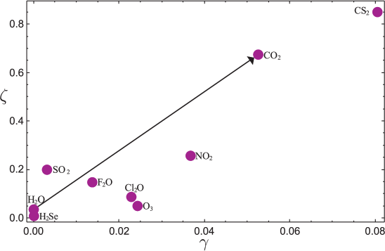
Figure 1: Location of several molecules in the diagram $\zeta$ vs $\gamma$. The arrow indicates the parameterization considered to study the LNT.

3 Local-to-Normal mode transition

In this section we shall analyze the LNT through the study of the stretching modes of a triatomic molecule modelled with a Hamiltonian of two interacting Morse oscillators. The Morse potential can be expressed as $V_{M}(q)=Dy^{2}$ with $y=1-e^{-\beta q}$. The number of quanta $v_{i}$ for each oscillator takes the values $v_{i}=0,1,\dots,j-1$ with $\kappa=2j+1$ related with the depth of the potential $D$. We introduce a linear parameterization in the $\{x_{g}\equiv t,x_{f}(t)\}$ space from the water parameters $(x_{g}^{(L)}=-0.015,x_{f}^{(L)}=-0.012)$ to the ones associated with the carbon dioxide $(x_{g}^{(N)}=-0.571,x_{f}^{(N)}=0.047)$. This parameterization induces the linear $t$-dependence for the frequency $\omega(t)=m_{\omega}t+w^{(N)}$and the Morse parameter $\kappa(t)=m_{\kappa}t+\kappa^{(N)}$, where $m_{\omega}=(\omega^{(N)}-\omega^{(L)})/(x_{g}^{(L)}-x^{(N)}_{g}),m_{\kappa}=(\kappa^{(N)}-\kappa^{(L)})/(x_{g}^{(L)}-x^{(N)}_{g})$, with $k^{(L)}=48$, $k^{(N)}=160$, and $\omega^{(L)}=1853$ cm^-1, $\omega^{(N)}=$ 959  cm^-1, which were chosen in order to reproduce the fundamentals. The $\beta(t)$ is given by $\beta(t)=\sqrt{[2w(t)]/[\hbar\kappa(t)g_{rr}^{\circ}(t)]}$. Then the Hamiltonian for the two interacting Morse oscillators takes the form

$$\hat{H}(t)= \hbar\omega(t)\bigg{\{}\sum_{i=1}^{2}\big{[}(\hat{v}_{i}+1/2)-{1\over\kappa(t)}(\hat{v}_{i}+1/2)^{2}\big{]}$$

$$+{2~{}t\over\kappa(t)}\hat{\bar{p}}_{1}\hat{\bar{p}}_{2}+{\kappa(t)~{}x_{f}(t)\over 2}\hat{y}_{1}\hat{y}_{2}\bigg{\}},$$ (4)

where here the momenta $\hat{\bar{p}}_{i}$ are dimensionless. We should stress that the space $|jv_{1}v_{2}\rangle$ is divided into two subspaces, the one belonging complete polyads and the rest belonging to the continuum [27].

The parameterization $\kappa(t)$ implies different dimensions for the Hamiltonian matrix representation. Since we are interested in the low lying region of the spectrum we have kept the dimension constant (consistent with $\kappa=10$), albeit changing $\kappa$ in accordance with $\kappa(t)$ in the calculation of the matrix elements. In this way we simplify the numerical description without losing physical content. In Fig. 2 we display the energy correlation diagram for the first $42$ symmetric eigenstates provided by the Hamiltonian (3). The left hand side corresponds to the local limit where a clear polyad preserving pattern is evident up to polyad $6$. In this limit the polyad in terms of local and normal number operators coincide $P_{N}=P_{L}$. As $|t|$ increases apparent level crossings appear suggesting the location of the LNT. We will show however that the transition is not determined by these crossings, but by properties carried by the eigenstates as the polyad $P_{L}$ is broken. There are several sensitive properties that provide a precise information for the transition region, on which we base our strategy:

a) Components. The analysis of the dominant components of the eigenkets in both local and normal basis should reflect the transition. The normal basis, however, deserves some discussion since strictly speaking a normal basis does not exist in a set of Morse oscillators. In order to extract from the eigenstates the components of the normal basis we construct the normal states diagonalizing the number operators $\{\hat{\nu}_{1},\hat{\nu}_{3}\}$ in the harmonic local basis $|n_{1}n_{2}\rangle$. The resulting transformation matrix is inverted to substitute the local basis in the Morse eigenstates with the following identification $|n_{1}n_{2}\rangle\to|jv_{1}v_{2}\rangle$. This approach is feasible as long as the maximum component of the eigenstates is located in the subspace of complete polyads.

b) Fidelity. Another property to extract information about the transition is through the fidelity $F_{\alpha}(t)$ associated with a given eigenstate $|\Psi_{\alpha}\rangle$, and defined as the overlap between consecutive eigenstates parametrically separated by $\delta t$: $F_{\alpha}(t)=|\langle\Psi_{\alpha};t|\Psi_{\alpha};t+\delta t\rangle|^{2}.$

c) Entropy. The transition may also be manifested through the entanglement between the two oscillators, a quantitative property measured calculating the entropy defined as [20]: $S_{\alpha}=-\sum_{i}\lambda_{i}\ln\lambda_{i},$ where $\lambda_{i}$ is the $i$-th eigenvalue of the matrix $||\langle jv_{1}^{\prime}|Tr_{2}\rho_{\alpha}|jv_{1}\rangle||$ with density operator $\rho_{\alpha}=|\Psi_{\alpha}\rangle\langle\Psi_{\alpha}|$, while $Tr_{2}\rho_{\alpha}=\sum_{v_{2}}\langle jv_{2}|\Psi_{\alpha}\rangle\-\langle\Psi_{\alpha}|jv_{2}\rangle$. In the local limit the entropy vanishes, and it increases as the coupling appears.

d) Probability density. We may also see the transition by plotting the probability density $\rho_{\alpha}$ associated with the eigenstate $|\Psi_{\alpha}\rangle$ in the coordinate representation: $\rho_{\alpha}(q_{1},q_{2})=|\langle q_{1}q_{2}|\Psi_{\alpha}\rangle|^{2}$. This property has proved to be useful in reflecting the local-normal character [7].

e) Poincaré sections. Since during the LNT the polyads $P_{L}$ and $P_{N}$ are not preserved, chaos is expected to appear [28, 29]. Consequently chaotic phase spaces in the polyad breaking regions should be manifested. In order to identify the transition, Poincaré sections will be relevant.

4 Analysis of the results

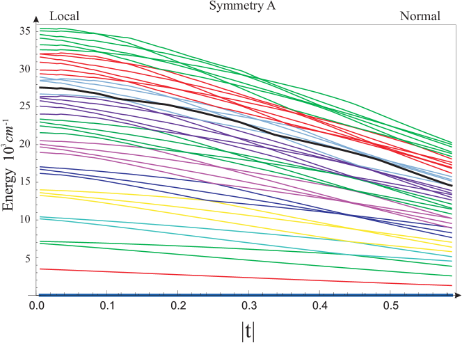
Figure 2: Energy correlation between the local and normal limits for the symmetric states for two interacting Morse oscillators.

We have chosen the states $\{26,27,28\}$ as a representative set displaying the main features of the energy spectrum by the set of interacting Morse oscillators. These states can be located in Fig. 2, where the state $27$ stands out in black. Although the whole range of the transition from water to carbon dioxide is displayed, we shall constraint our analysis in the upper left part of the spectrum in the interval $|t|\in[0.0147,0.2]$, since it is in this region where the LNT is manifested in different forms. In Fig. 3a a zoom of the three levels is shown. Although at first sight crossing of levels appears, a more detailed analysis shows that they are avoided crossings [25, 26].

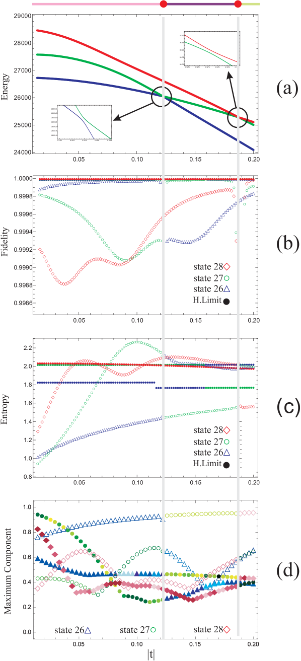
Figure 3: Properties of the set of states $\{26,27,28\}$ in the interval $t[-0.014,-0.2]$: (a) Energies, (b) Fidelity, (c) Entropy and (d) Maximum local and normal components. In panel (d) full figures corresponds to maximum local components, while the corresponding empty figure refers to the normal component.

The approaching of levels in the spectrum suggests a polyad breaking effect, but it does not provide a precise information about the region where it takes place. In Fig. 3b the fidelity is displayed for the three states. As a reference the avoided crossings are marked with vertical lines in gray. While states $27$ and $28$ show a sensitive behavior under this property, state $26$ presents a small change, very close to the harmonic limit until the the first avoided crossing appears. This is explained by the existing competition between local and normal character of the eigenstates displayed in panel (d). The fidelity detects slope component changes which may appear near or at the crossings of the local-normal maximum components, manifested along the transition. At the locations of avoided crossings, the fidelity curves of the states $26$ and $27$ are interchanged indicating state crossings. A similar situation appears at the second point, where the states $27$ and $28$ are interchanged. These crossings appear along the transition because we are in a high energy region, but at low energies where no crossings appear, the properties displayed also detect the LNT in the same parametric region.

In Fig. 3c the entropy is exhibited for the three states. In the pure local limit the entanglement and consequently the entropy is expected to vanish, this explains its small values near H₂O. As we move to the CO₂ parameters there is an entropy change associated with the LNT with features closely related to the local maximum component. After the transition the entropy of the states tend to the harmonic limit, which corresponds to constant values of the entropy. Here the avoided crossings are also manifested.

In Fig. 3d we present the square of the maximum component in both local and normal bases. The local components correspond to filled figures. The state $27$ starts with an almost purely local character (0.95). As $|t|$ increases the local character rapidly diminishes with a proportional increasing of entropy. A similar situation appears in the state $28$, although in this case a maximum and minimum appears, in accordance to the local maximum component behavior. In contrast, the state $26$ does not present such change in the first part, but after the crossing a change of dominance appears and detected by the fidelity. Hence fidelity and entropy reflects in different form the subtle changes in the character of the eigenstates.

A picture of the studied states can be obtained by plotting the probability density distribution in the coordinate representation. In Fig. 4 the probability density is shown for the three states as a function of the parameter $t$. The crossing points are indicated with full circles. Except for the state $26$, the other two states present an evident local character with the parameters of water molecule. The state $26$ contains a mixed character, a feature reflected by the components in Fig. 3d. As $|t|$ increases, the transformation to NM character becomes manifest. This visual point of view however is quite imprecise since after the first crossing the change in the probability densities stop being noticeable, in contrast to the fidelity which continue detecting changes. The analysis of the plots before and after the red circles (avoided crossings) shows clearly that a crossing of states takes place [25, 26]. At the crossing points a small change in the probability densities is revealed, although in general it will depend on the energy region as well as on the value of the parameter.

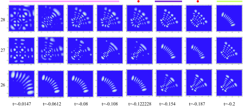
Figure 4: Probability densities for the set of states $\{26,27,28\}$ as a function of the parameter $x_{g}$. The avoided energy crossings are indicated with a red circles.

Finally in Fig. 5, the Poincaré sections for the state $27$ are shown for different values of the parameter. Each plot is associated with the corresponding energy in Fig. 2, in such a way that it changes as we move to the normal limit represented by CO₂. In these plots we notice that the LNT is manifested by a chaotic behavior. This is reasonable because the appearance of chaos has been associated with lacking of preserved quantities like the polyad number [32, 31]. In the local limit we have integrable trajectories as well as in the normal limit. In the former case the polyad $P_{L}$ is preserved, while in the latter $P_{N}$ is a good quantum number. Hence it is in between, where the transition takes place, manifested with the appearance of chaos. In Fig. 5 only the state $27$ is analyzed because the other two states are so close in energy that classically they do not provide additional information. Although the chaotic transient regime associated with Poincaré sections is energy dependent, we can establish that a global chaotic regime indicates the LNT in more precise terms, something that we cannot say just with the condition (2). Notice that while the analysis leading to the condition (2) was based on the harmonic limit, the study in terms of Morse oscillators display the transition regime as suggested.

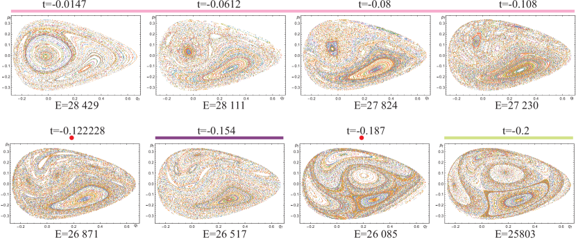
Figure 5: Poincaré sections for the state $27$ as a function of the parameter $x_{g}$.

Appearance of chaos in a system of interacting Morse oscillators has been detected previously by considering different coupling strengths. Since working with exact interacting Morse oscillators involves the appearance of all the resonances [33], Poincaré sections are displayed in Ref.[31] to elucidate the appropriate approximation which preserve the essential features of the system. Coupling strength in the kinetic energy is related to masses and geometry of the system. Increasing this coupling may be interpreted either by a mass ratio and/or geometry modifications. In this sense the appearance of chaos in Refs. [30, 31, 32] may be interpreted as parametric transformations in the same direction as the presented analysis. Our work however address the polyad breaking phenomenon in search of regions where a system cannot be considered neither normal nor local, which is precisely associated with the appearance of chaos.

5 Conclusions

In this work we have identified the LNT taking into account that the condition $P_{L}=P_{N}$ is not valid in the whole range of force and structure constants. The LNT has been studied using a 1D parametric form of the Hamiltonian for two interacting Morse oscillators. This system was chosen because it carries the main ingredients to successfully describe molecules with a LM behavior. The parametric form was based on the transformation from water to carbon dioxide molecule, through the set $\{x_{g},x_{f},\kappa\}$ of parameters in linear form. Although in our analysis the transition can be identified with a specific range of the parameter $x_{g}$, the transition features vary with the energy. This analysis differs from the previous studies of LMT in the sense that we are evaluating the range of parameters where the local force constants cannot be estimated using a local model, a region where the polyad $P_{L}$ stop being preserved.

The transition was studied using several properties which proved to furnish significant physical insight into the molecular behavior. The fidelity is a sensitive property that detects slope changes in the maximum components of the eigenstates. On the other hand the entropy reflects the local character of the eigenstates by its increasing when the local character diminishes. These properties are complementary and provide the relevant interval of the transition, but also the detailed transformation undergone by the eigenstates.

The probability densities were also analyzed during the transition, which it is not manifested in all the states. From the correlation diagram we detect avoiding crossings. These crossings do not establish a signature of the transition and appear as a consequence of the high energy region analyzed. States of lower energy undergo the transition in the same region without presenting any crossing. Finally a semiclassical feature of our analysis is the identification of a clear LNT interval through the appearance of chaos coinciding with the the abrupt changes in fidelity and entropy.

- [1] \NameKellman M.E. \BookJ.Chem.Phys. \Vol93 \Page 6630 \Year(1990).
- [2] \NamePapouek D. Aliev M.R. \BookMolecular Vibrational-Rotational Spectra \EditorElsevier \Year(1982)
- [3] \NameKellman M.E. \Book Annu. Rev. Phys. Chem. \Vol 46 \Year(1995) \Page 395.
- [4] \NameBunker P.R. JensenP. \BookMolecular Symmetry and Spectroscopy \EditorNational Research Council of Canada \Year(1998)
- [5] \NameChild M.S. Lawton R.T. \BookFaraday Discuss. Chem. Soc. \Vol71 \Year(1981) \Page273.
- [6] \NameJensen P. \BookMol.Phys. \Vol 98 \Page1253 \Year(2000)
- [7] \NameChild M.S. Halonen L. \Book Adv.Chem.Phys. \Vol 57 \Page1 \Year(1984)
- [8] \NameHalonen L. \BookComputational Molecular Spectroscopy \EditorJohn Wiley and Sons \Year(2000)
- [9] \NameT.Sako, et al \BookJ.Phys.Chem. \Vol 113 \Page7292 \Year(2000)
- [10] \NameT.Sako, et al \BookJ.Phys.Chem. \Vol 117 \Page1641 \Year(2002)
- [11] \NameE.L.Sibert III, et al \BookJ.Chem.Phys. \Vol 77 \Page3595 \Year(1982)
- [12] \NameM.J.Davis \BookIn.Rev.Phys.Chem. \Vol 14 \Page15 \Year(1995)
- [13] \NameE.J.Heller and M.J.Davis \BookJ.Phys.Chem. \Vol 84 \Page1999 \Year(1980)
- [14] \NameKellman M.E. Tyng V. \BookAcc.Chem.Res. \Vol 40 \Page243 \Year(2007)
- [15] \NameKellman M.E. \BookJ.Chem.Phys. \Vol89 \Page6087 \Year(1989)
- [16] \NameG.M.Schmid, et al \BookChem.Phys.Lett. \Vol 219 \Page331 \Year(1994)
- [17] \NameKellman M.E. Lynch E.D. \BookJ.Chem.Phys. \Vol88 \Page2205 \Year(1988)
- [18] \NameSako T. et al \BookJ.Chem.Phys. \Vol114 \Page9441 \Year(2001)
- [19] \NameShao L. Kellman M. \BookJ.Chem.Phys. \Vol93 \Page5805 \Year(1990)
- [20] \NameBenenti G. et al \BookPrinciples of Quantum Computation and Information \EditorWorld Scientific \Year(2004)
- [21] \NameCastaños O. et al \Book J. Phys: Conf. Ser. 387 (2012) 012021; 403 (2014) 012003.
- [22] \NameRomera E. et al \BookPhys. Scr. \Vol 89 \Year(2014) \Page095103
- [23] \NameMills M. Rpbiette G. \BookMol.Phys. \Vol56 \Year(1985) \Page743
- [24] \NameLemus R. et al \BookJ.Chem.Phys. \Vol141 \Page054306 \Year(2014)
- [25] \NameS.Keshavamurty \BookJ.Phys.Chem.A \Vol105 \Page2668 \Year(2001)
- [26] \NameS.Yang and M.E.Kellman \BookPhys.Rev.A \Vol81 \Page062512 \Year(2010)
- [27] \NameAlvarez-Bajo O. et al \BookMol.Phys. \Vol106 \Year(2008) \Page1275
- [28] \NameLu LZ.M. and Kellman M.E. \BookJ.Chem.Phys. \Vol107 \Page1 \Year(1997)
- [29] \NameKeshavamurthy M.E. S. EzraG. S. \BookJ.Chem.Phys. \Vol107 \Page156 \Year(1997)
- [30] \NameMatsushita T. Terasaka T \BookChem.Phys. Lett. \Vol100 \Page138 1983
- [31] \NameJung C. et al \BookChaos \Vol11 \Page464 \Year(2001)
- [32] \NameChakraborty A. Kellman M.E. \BookJ.Chem.Phys. \Vol129 \Page171104 \Year (2008)
- [33] \NameJaffé Ch. Brumer P. \BookJ.Chem.Phys. \Vol73 \Page5647 \Year(1980)