Distance distribution in configuration model networks

Abstract

We present analytical results for the distribution of shortest path lengths between random pairs of nodes in configuration model networks. The results, which are based on recursion equations, are shown to be in good agreement with numerical simulations for networks with degenerate, binomial and power-law degree distributions. The mean, mode and variance of the distribution of shortest path lengths are also evaluated. These results provide expressions for central measures and dispersion measures of the distribution of shortest path lengths in terms of moments of the degree distribution, illuminating the connection between the two distributions.

I Introduction

The study of complex networks has attracted much attention in recent years. It was found that network models provide a useful description of a large number of processes which involve interacting objects Barabasi2002 ; Caldarelli2007 ; Havlin2010 ; Newman2010 ; Estrada2011 . In these models, the objects are represented by nodes and the interactions are expressed by edges. Pairs of adjacent nodes can affect each other directly. However, the interactions between most pairs of nodes are indirect, mediated by intermediate nodes and edges.

A pair of nodes, $i$ and $j$, may be connected by a large number of paths. The shortest among these paths are of particular importance because they are likely to provide the fastest and strongest interaction. Therefore, it is of interest to study the distribution of shortest path lengths (DSPL) between pairs of nodes in different types of networks. Such distributions, which are also referred to as distance distributions, are expected to depend on the network structure and size. They are of great importance for the temporal evolution of dynamical processes on networks, such as signal propagation Maayan2005 , navigation Dijkstra1959 ; Delling2009 ; Abraham2013 and epidemic spreading Satorras2001 ; Satorras2015 . Central measures of the DSPL such as the average distance between pairs of nodes, and extremal measures such as the diameter were studied Bollobas2001 ; Watts1998 ; Fronczak2004 . However, apart from a few studies Newman2001 ; Blondel2007 ; Dorogotsev2003 ; Hofstad2007 ; Hofstad2008 ; Esker2008 , the entire DSPL has attracted little attention.

Recently, an analytical approach was developed for calculating the DSPL Katzav2015 in the Erdős-Rényi (ER) network, which is the simplest mathematical model of a random network Erdos1959 ; Erdos1960 ; Erdos1961 . Using recursion equations, analytical results for the DSPL were obtained in different regimes, including sparse and dense networks of small as well as asymptotically large sizes. The resulting distributions were found to be in good agreement with numerical simulations.

ER networks are random graphs in which the degrees follow a Poisson distribution and there are no degree-degree correlations between connected pairs of nodes. In fact, ER networks can be considered as a maximum entropy ensemble under the constraint that the mean degree is fixed. Moreover, there is a much broader class of networks, named the configuration model, which generates maximum entropy ensembles when the entire degree distribution is constrained Newman2010 ; Newman2001 ; Fronczak2004 ; Molloy1995 . The ER ensemble is equivalent to a configuration model in which the degree distribution is constrained to be a Poisson distribution. For any given degree distribution, one can produce an ensemble of configuration model networks and perform a statistical analysis of its properties. Therefore, the configuration model provides a general and highly powerful platform for the analysis of networks. It is the ideal model to use as a null model when one tries to analyze an empirical network of which the degree distribution is known. For a given empirical network, one constructs a configuration model network of the same size and the same degree distribution. Properties of interest such as the DSPL Giot2003 , the betweenness centrality Goh2003 and the abundance of network motifs Milo2002 are compared between the two networks. The differences provide a rigorous test of the systematic features of the empirical network vs. the random network.

A theoretical framework for the study of the shell structure in configuration model networks was developed in a series of papers Kalisky2006 ; Shao2008 ; Shao2009 . The shell structure around the largest hub in a scale free network was analyzed in Ref. Kalisky2006 . This approach was later extended into a general theory of the shell structure arond a random node in a configuration model network Shao2008 ; Shao2009 . This formulation is based on recursion equations for the number of nodes in each shell and for the degree distributions in the shells. In the special case of the ER network, the results of Refs. Shao2008 ; Shao2009 for the number of nodes in each shell coincide with those of Ref. Blondel2007 .

The shell structure around a random node in the configuration model was recently utilized for the study of epidemic spreading Shao2015 . In a study of biological networks, the DSPL in a protein-protein interaction network was analyzed and compared to a corresponding configuration model network Giot2003 . It was found that the distances in the configuration model are shorter than in the original empirical network. This highlights the features of the biological network which tend to increase the distances. These studies demonstrate the applicability of the configuration model in the analysis of the structure and dynamics in empirical networks.

In this paper we develop a theoretical framework, based on the cavity approach Mezard1985 ; Mezard2003 ; Mezard2009 ; Ferraro2013 , for the calculation of the DSPL in networks which belong to the configuration model class. Using this framework we derive recursion equations for the calculation of the DSPL in configuration model networks. We apply these equations to networks with degenerate, binomial and power-law degree distributions, and show that the results are in good agreement with numerical simulations. Using the tail-sum formula we calculate the mean and the variance of the DSPL. Evaluating the discrete derivative of the tail distribution, we also obtain the mode of the DSPL. These results provide closed form expressions for the central measures and dispersion measures of the DSPL in terms of the moments of the degree distribution and the size of the network, illuminating the connection between the two distributions.

The paper is organized as follows. In Sec. II we present the class of configuration model networks. In Sec. III we use the cavity approach to derive the recursion equations for the calculation of the DSPL in these networks. In Sec. IV we consider properties of the DSPL such as the mean, mode and variance. In Sec. V we present the results obtained from the recursion equations for different network models and compare them to numerical simulations. In Sec. VI we present a summary of the results.

II The configuration model

The configuration model is a maximum entropy ensemble of networks under the condition that the degree distribution is imposed Newman2001 ; Newman2010 . Here we focus on the case of undirected networks, in which all the edges are bidirectional. To construct such a network of $N$ nodes, one can draw the degrees of all nodes from a desired degree distribution $p(k)$, $k=0,1,\dots,N-1$, producing the degree sequence $k_{i}$, $i=1,\dots,N$ (where $\sum k_{i}$ must be even). The degree distribution $p(k)$ satisfies $\sum_{k}p(k)=1$. The mean degree over the ensemble of networks is $c=\langle k\rangle=\sum_{k}kp(k)$, while the average degree for a single instance of the network is $\bar{k}=\sum_{i}k_{i}/N$. Here we consider networks which do not include isolated nodes, namely $p(0)=0$. This does not affect the applicability of the results, since the distribution of shortest path lengths is evaluated only for pairs of nodes which reside on the same cluster, for which the distance is finite. Actually, if a network includes isolated nodes, one can discard them by considering a renormalized degree distribution of the form $p(k)/[1-p(0)]$, for $k=1,\dots,N-1$.

A convenient way to construct a configuration model network is to prepare the $N$ nodes such that each node, $i$, is connected to $k_{i}$ half edges Newman2010 . Pairs of half edges from different nodes are then chosen randomly and are connected to each other in order to form the network. The result is a network with the desired degree sequence but no correlations. Note that towards the end of the construction the process may get stuck. This may happen in case that the only remaining pairs of half edges are in the same node or in nodes which are already connected to each other. In such cases one may perform some random reconnections in order to enable completion of the construction.

III Derivation of the recursion equations

Consider a random pair of nodes, $i$ and $j$, in a network of $N$ nodes. Assuming that the two nodes reside on the same connected cluster, they are likely to be connected by a large number of paths. Here we focus on the shortest among these paths (possibly more than one). More specifically, we derive recursion equations for the length distribution of these shortest paths. To this end we introduce the indicator function

$$\chi_{N}(d_{ij}>\ell)=\left\{\begin{array}[]{ll}1&d_{ij}>\ell\\ 0&d_{ij}\leq\ell,\end{array}\right.$$ (1)

where $d_{ij}$ is the length of the shortest path between nodes $i$ and $j$, and $\ell$ is an integer. We also introduce the conditional indicator function

$$\chi_{N}(d_{ij}>\ell|d_{ij}>\ell-1)=\frac{\chi_{N}(d_{ij}>\ell\cap d_{ij}>\ell-1)}{\chi_{N}(d_{ij}>\ell-1)}.$$ (2)

Under the condition that the length $d_{ij}$ is larger than $\ell-1$, this function indicates whether $d_{ij}$ is also larger than $\ell$. If it is, the conditional indicator function $\chi=1$, otherwise (namely if $d_{ij}=\ell$) $\chi=0$. In case the condition $d_{ij}>\ell-1$ is not satisfied, the value of the conditional indicator function is undetermined. In order to extend this definition we adopt the convention that in case the condition is not satisfied the conditional indicator function takes the value $\chi_{N}(d_{ij}>\ell|d_{ij}>\ell-1)=1$. We note that all the subsequent results are independent of the value adopted here. The indicator function $\chi_{N}(d_{ij}>\ell)$ can be expressed as a product of the conditional indicator functions in the form

$$\chi_{N}(d_{ij}>\ell)=\chi_{N}(d_{ij}>0)\prod_{\ell^{\prime}=1}^{\ell}\chi_{N}(d_{ij}>\ell^{\prime}|d_{ij}>\ell^{\prime}-1),$$ (3)

where $\chi_{N}(d_{ij}>0)=1$, since $i$ and $j$ are assumed to be two different nodes.

In the analysis below we calculate the mean of the indicator function over an ensemble of networks to obtain the distribution of shortest path lengths $P_{N}(d>\ell)$. To this end we define the mean conditional indicator function $m_{i}(\ell)\in[0,1]$, obtained by averaging the conditional indicator function $\chi_{N}(d_{ij}>\ell|d_{ij}>\ell-1)$ over all suitable choices of the final node, $j$:

$$m_{i}(\ell)={\langle\chi_{N}(d_{ij}>\ell|d_{ij}>\ell-1)\rangle}_{j}.$$ (4)

The averaging is done only over nodes $j$ which reside on the same cluster as node $i$ and for which the condition $d_{ij}>\ell-1$ is satisfied.

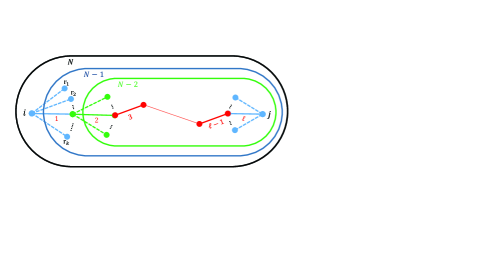
A path of length $\ell$ from node $i$ to node $j$ can be decomposed into a single edge connecting node $i$ and node $r\in\partial_{i}$ (where $\partial_{i}$ is the set of all nodes directly connected to $i$), and a shorter path of length $\ell-1$ connecting $r$ and $j$. Thus, the existence of a path of length $\ell$ between nodes $i$ and $j$ can be ruled out if there is no path of length $\ell-1$ between any of the nodes $r\in\partial_{i}$, and $j$ (Fig. 1). The conditional indicator functions for these paths of length $\ell-1$ are $\chi_{N-1}^{(i)}(d_{rj}>\ell-1|d_{rj}>\ell-2)$, since they are embedded in a smaller network of $N-1$ nodes, which does not include node $i$. The superscript $(i)$ stands for the fact that the node $r$ is reached by a link from node $i$. This is often referred to as the cavity indicator function Mezard1985 ; Mezard2003 ; Mezard2009 ; Ferraro2013 . Similarly, we define the mean cavity indicator function as

$$m_{r}^{(i)}(\ell)={\langle\chi^{(i)}_{N}(d_{rj}>\ell|d_{rj}>\ell-1)\rangle}_{j}.$$ (5)

This reasoning enables us to express the conditional indicator function $\chi_{N}(d_{ij}>\ell|d_{ij}>\ell-1)$ as a product of conditional indicator functions for shorter paths between nodes $r\in\partial_{i}$ and $j$

$$\chi_{N}(d_{ij}>\ell|d_{ij}>\ell-1)=\prod_{r\in\partial_{i}\texttt{\char 92\relax}\{j\}}\chi_{N-1}^{(i)}(d_{rj}>\ell-1|d_{rj}>\ell-2).$$ (6)

Under the assumption that the local structure of the network is tree-like, one can approximate the average of the product in Eq. (6) by the product of the averages. This assumption is fulfilled in the limit of large networks. In the analysis below we assume that $N\rightarrow\infty$ and thus obtain recursion equations of the form

$$m_{i}(\ell)=\prod_{r\in\partial_{i}\texttt{\char 92\relax}\{j\}}m_{r}^{(i)}(\ell-1).$$ (7)

The mean cavity indicator function $m_{r}^{(i)}(\ell)$ obeys a similar equation of the form

$$m_{r}^{(i)}(\ell)=\prod_{s\in\partial_{r}\texttt{\char 92\relax}\{i,j\}}m_{s}^{(r)}(\ell-1).$$ (8)

The number of neighbors $r\in\partial_{i}$ is given by the degree, $k_{i}$, of node $i$, while the number of neighbors $s\in\partial_{r}$ is given by the degree, $k_{r}$, of node $r$. Node $i$ is a randomly chosen node and thus its degree, $k_{i}$, is drawn from $p(k)$. Node $r$ is an intermediate node along the path and its probability to be encountered is proportional to its degree. Thus, its degree, $k_{r}$, is drawn from the distribution $(k/c)p(k)$, where $c$ takes care of the normalization.

Considering an ensemble of networks, the variables $m_{i}(\ell)$ and $m_{r}^{(i)}(\ell)$, which were defined for a specific node, $i$, on a given instance of the network, turn into the random variables $m(\ell)$ and $\tilde{m}(\ell)$, respectively. These random variables are drawn from suitable probability distributions, which respect the recursion equations (7) and (8). We denote these distributions by $\pi_{\ell}(m)=Pr[m(\ell)=m]$ and $\tilde{\pi}_{\ell}(m)=Pr[\tilde{m}(\ell)=m]$. These distributions obey the equations

$$\pi_{\ell}(m)=\sum_{k=1}^{\infty}p(k)\int_{0}^{1}\int_{0}^{1}\dots\int_{0}^{1}\prod_{\nu=1}^{k}\tilde{\pi}_{\ell-1}(m_{\nu}){\rm d}m_{\nu}\delta\left(m-\prod_{\nu=1}^{k}m_{\nu}\right)$$ (9)

and

$$\tilde{\pi}_{\ell}(m)=\sum_{k=1}^{\infty}\frac{k}{c}p(k)\int_{0}^{1}\int_{0}^{1}\dots\int_{0}^{1}\prod_{\nu=1}^{k-1}\tilde{\pi}_{\ell-1}(m_{\nu}){\rm d}m_{\nu}\delta\left(m-\prod_{\nu=1}^{k-1}m_{\nu}\right).$$ (10)

Eq. (9) refers to the random node, $i$, thus its degree is drawn from $p(k)$. Eq. (10) refers to intermediate nodes along the path, thus the degrees are drawn from the distribution $(k/c)p(k)$. An additional feature of the intermediate nodes is that one of their edges is consumed by the incoming link, leaving only $k-1$ links for the outgoing paths.

The expectation values of $m(\ell)$ and $\tilde{m}(\ell)$ over the graph ensemble yield the conditional probabilities

$$m_{\ell}=P(d>\ell|d>\ell-1)=\int_{0}^{1}m\pi_{\ell}(m){\rm d}m$$ (11)

and

$$\tilde{m}_{\ell}=\tilde{P}(d>\ell|d>\ell-1)=\int_{0}^{1}m\tilde{\pi}_{\ell}(m){\rm d}m.$$ (12)

Plugging Eqs. (9) and (10) into Eqs. (11) and (12), respectively, we obtain the recursion equations

$$m_{\ell}=\sum_{k=1}^{\infty}p(k)(\tilde{m}_{\ell-1})^{k}$$ (13)

and

$$\tilde{m}_{\ell}=\sum_{k=1}^{\infty}\frac{k}{c}p(k)(\tilde{m}_{\ell-1})^{k-1},$$ (14)

which are valid for $\ell\geq 2$. Recalling that $p(0)=0$, Eqs. (13) and (14) can be written using the degree generating functions Newman2001

$$m_{\ell}=G_{0}\left(\tilde{m}_{\ell-1}\right)$$ (15)

and

$$\tilde{m}_{\ell}=G_{1}\left(\tilde{m}_{\ell-1}\right),$$ (16)

where

$$G_{0}(x)=\sum_{k=0}^{\infty}p(k)x^{k}$$ (17)

and

$$G_{1}(x)=\sum_{k=0}^{\infty}\frac{k}{c}p(k)x^{k-1}.$$ (18)

Eq. (13) can be understood intuitively as follows. Consider the simplified scenario in which node $i$ is known to have a degree $k$. In this case, excluding a path of length $\ell$ from $i$ to $j$ is equivalent to excluding a path of length $\ell-1$ from all $k$ neighbors of $i$ to $j$, namely $m_{\ell}=(\tilde{m}_{\ell-1})^{k}$. Such reasoning was applied in Ref. Katzav2015 , to obtain the DSPL from a node with a given degree to all other nodes in the network. In practice, the degree of a random node is unknown, and is distributed according to $p(k)$. Therefore, Eq. (13) averages over all possible degrees with suitable weights, provided by $p(k)$. Eq. (14) can be understood using a similar reasoning.

In the case of finite networks, we obtain

$$m_{N,\ell}=\sum_{k=1}^{N-2}p(k)(\tilde{m}_{N-1,\ell-1})^{k}$$ (19)

and

$$\tilde{m}_{N,\ell}=\sum_{k=1}^{N-2}\frac{k}{c}p(k)(\tilde{m}_{N-1,\ell-1})^{k-1},$$ (20)

for $\ell\geq 2$. For $\ell=1$ we can directly obtain the results

$$m_{N,1}=\sum_{k=1}^{N-1}p(k)\left(1-\frac{1}{N-1}\right)^{k}$$ (21)

and

$$\tilde{m}_{N,1}=\sum_{k=1}^{N-1}\frac{k}{c}p(k)\left(1-\frac{1}{N-1}\right)^{k-1}.$$ (22)

The tail distribution of the shortest path lengths can be expressed as a product of the form

$$P_{N}(d>\ell)=P_{N}(d>0)\prod_{\ell^{\prime}=1}^{\ell}P_{N}(d>\ell^{\prime}|d>\ell^{\prime}-1)\equiv P_{N}(d>0)\prod_{\ell^{\prime}=1}^{\ell}m_{N,\ell^{\prime}}.$$ (23)

Actually, since we choose two different nodes as the initial and final nodes, $P_{N}(d>0)=1$, which further simplifies Eq. (23).

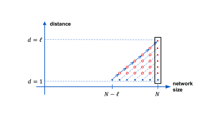
In Fig. 2 we illustrate the way the recursion equations are iterated $\ell^{\prime}-1$ times along the diagonal in order to obtain $m_{N,\ell^{\prime}}$. Starting from $\tilde{m}_{N-\ell^{\prime},1}$ (squares), Eq. (20) is iterated $\ell^{\prime}-2$ times (empty circles), followed by a single iteration (full circles) of Eq. (19). The desired value of $P_{N}(d>\ell)$ is obtained from Eq. (23). This product runs from bottom to top along the rightmost column of Fig. 2.

The probability distribution function, namely, the probability $P_{N}(\ell)=P_{N}(d=\ell)$ that the shortest path length between a random pair of nodes is equal to $\ell$ can be obtained from the tail distribution by

$$P_{N}(\ell)=P_{N}(d>\ell-1)-P_{N}(d>\ell),$$ (24)

for $\ell=1,2,\dots,N-1$.

It should be noted that Eqs. (9) and (10), presenting the distributions $\pi_{\ell}(m)$ and $\tilde{\pi}_{\ell}(m)$ enable the analysis of fluctuations of the conditional probabilities within an ensemble of networks with a given degree distribution in the large $N$ limit.

IV Properties of the DSPL

The distribution of shortest path lengths, $P_{N}(\ell)$, can be characterized by its moments. The $n$th moment, $\langle\ell^{n}\rangle$, can be obtained using the tail-sum formula Pitman1993

$$\langle\ell^{n}\rangle=\sum_{\ell=0}^{N-2}[(\ell+1)^{n}-\ell^{n}]P_{N}(d>\ell).$$ (25)

Note that the sum in Eq. (25) does not extend to $\infty$ because the longest possible shortest path in a network of size $N$ is $N-1$. The average distance between pairs of nodes in the network is given by the first moment

$$\langle\ell\rangle=\sum_{\ell=0}^{N-2}P_{N}(d>\ell).$$ (26)

The average distance between nodes in configuration model networks has been studied extensively Newman2001 ; Chung2002 ; Chung2003 ; Hofstad2005 ; Esker2006 ; Bollobas2007 ; Hofstad2007 ; Esker2008 . It was found that

$$\langle\ell\rangle\simeq\frac{\ln N}{\ln\left(\frac{\langle k^{2}\rangle-\langle k\rangle}{\langle k\rangle}\right)}+{\cal O}(1).$$ (27)

The width of the distribution can be characterized by the variance $\sigma_{\ell}^{2}=\langle\ell^{2}\rangle-\langle\ell\rangle^{2}$, where

$$\langle\ell^{2}\rangle=\sum_{\ell=0}^{N-2}(2\ell+1)P_{N}(d>\ell).$$ (28)

In addition to the average distance $\langle\ell\rangle$, another common measure of the typical distance between nodes in the network is the mode. Here we present a way to extract the mode of $P_{N}(\ell)$ directly from the recursion equations, in the limit of a large network. It is based on the following observations: (a) The tail-distribution, $P_{N}(d>\ell)$, is a sigmoid function, i.e. it starts at $1$ at the origin and drops to $0$ at infinity. The transition between the two levels occurs over a relatively narrow interval; (b) Actually, $P_{N}(d>\ell)$ can be expressed as a product of conditional probabilities of the form $m_{N,\ell^{\prime}}$, where each term has the form of a sigmoid function [Eq. (23)]. Therefore, the product becomes an even sharper sigmoid function, and to a good approximation its maximal slope is determined by the the last term in the product. Therefore, in the analysis below we focus on the conditional probability $m_{N,\ell}$.

Considering the large $N$ limit we can use the recursion equations (15) and (16). The generating functions satisfy $G_{0}(1)=G_{1}(1)=1$, thus both equations exhibit a (repelling) fixed point at $m_{\ell}=\tilde{m}_{\ell}=1$. Note that in this formulation, the network size $N$ does not appear explicitly in the recursion equations, but only enters through the initial conditions, given by Eqs. (21) and (22). For simplicity, we approximate Eqs. (21) and (22) by

$$m_{1}\simeq 1-\frac{c}{N-1}+{\cal O}\left(\frac{1}{N^{2}}\right),$$ (29)

and

$$\tilde{m}_{1}\simeq 1-\frac{\langle k^{2}\rangle-\langle k\rangle}{\langle k\rangle(N-1)}+{\cal O}\left(\frac{1}{N^{2}}\right),$$ (30)

respectively. For networks which are not too dense, these values are only slightly smaller than $1$. Therefore, the linearized versions of Eqs. (15) and (16) hold as long as $m_{\ell}$ and $\tilde{m}_{\ell}$ are sufficiently close to $1$. Note that these expressions require that the second moment $\langle k^{2}\rangle$ would be finite. This condition may limit the validity of the derivation presented below to networks for which $\langle k^{2}\rangle$ is bounded. Thus, networks for which $\langle k^{2}\rangle$ diverges require special attention.

The location of the maximum value of the probability distribution function (namely the mode) is obtained at the point where the tail distribution falls most sharply. Up to that point the linear approximation holds quite well. This motivates us to perform the analysis in terms of the deviations

$$\epsilon_{\ell}=1-m_{\ell},$$ (31)

and

$$\tilde{\epsilon}_{\ell}=1-\tilde{m}_{\ell}.$$ (32)

Linearizing Eqs. (15) and (16) in terms of $\epsilon_{\ell}$ and $\tilde{\epsilon}_{\ell}$, respectively, we obtain

$$\epsilon_{\ell}=\langle k\rangle\tilde{\epsilon}_{\ell-1},$$ (33)

and

$$\tilde{\epsilon}_{\ell}=\left[\frac{\langle k^{2}\rangle-\langle k\rangle}{\langle k\rangle}\right]^{\ell-1}\tilde{\epsilon}_{1},$$ (34)

for any $\ell\geq 2$, where $\tilde{\epsilon}_{1}={(\langle k^{2}\rangle-\langle k\rangle)}/{[\langle k\rangle(N-1)]}$. Our aim is to determine the value of $\ell$ at which the reduction in $m_{\ell}$ is maximal. We denote the discrete derivative

$$\Delta P=m_{\ell-1}-m_{\ell}.$$ (35)

Using the recursion equations (15) and (16), we can express this as

$$\Delta P=G_{0}(\tilde{m}_{\ell-2})-G_{0}[G_{1}(\tilde{m}_{\ell-2})],$$ (36)

and we are therefore interested in the value of $x$, denoted by $x_{max}$, at which the function $\Delta P(x)=G_{0}(x)-G_{0}[G_{1}(x)]$ is maximal. This is determined by the solution of the extremum condition

$$\frac{d\Delta P}{dx}=G_{0}^{\prime}(x)-G_{0}^{\prime}[G_{1}(x)]G_{1}^{\prime}(x)=0.$$ (37)

As long as $x_{max}$ is close to $1$ we can use the linear approximation leading to Eq. (34), in which case we can equate $\tilde{\epsilon}_{\ell_{mode}-2+{\cal O}(1)}=1-x_{max}$, where the ${\cal O}(1)$ term comes from the fact that we are using a linearized equation while potentially higher order corrections should have been considered. This term is small and could be omitted when $x_{max}$ is close to $1$, which is the situation in various known cases. Combining this result with Eq. (34) we obtain

$$\ell_{mode}=\frac{\ln\left[(N-1)(1-x_{max})\right]}{\ln\left(\frac{\langle k^{2}\rangle-\langle k\rangle}{\langle k\rangle}\right)}+2+{\cal O}(1).$$ (38)

It is interesting to note that the mode exhibits the same scaling with the network size as the average distance shown in Eq. (27). This analysis is in the spirit of the renormalization group approach, where the flow of an initial small deviation from the critical temperature (here from the fixed point $m=1$), under the linearized renormalization transformation determines the scaling behaviour of the system.

V Analysis of Network Models

To examine the recursion equations we apply them to the calculation of the DSPL in configuration model networks with different choices of the degree distribution. The results are compared to numerical simulations. In these simulations we generate instances of the configuration model networks with the required degree distribution. We then calculate the distances between all pairs of nodes in each network and generate a histogram. The process is repeated over a large number network instances. In case that the network includes more than one connected cluster we take into account only the distances between pairs of nodes which reside on the same cluster. The DSPL obtained from the numerical simulations is normalized accordingly.

To cover a broad class of networks, we consider configuration models which exhibit narrow as well as broad degree distributions. For networks with narrow degree distributions we study the the regular network (degenerate distribution) and networks with a binomial distribution. For networks with broad degree distributions we study configuration models with power-law degree distributions (scale-free networks). A detailed analysis of the distributions of shortest path lengths in these configuration models is presented below.

V.1 Regular Networks

The simplest case of the configuration model is the regular graph, in which the degree distribution is $p(k)=\delta_{k,c}$, namely all $N$ nodes have the same degree, (where $c\geq 2$ and $Nc$ is even). For $c=2$ the network consists only of loops, while for $c\geq 3$ more complex network structures appear. The random regular graph ensemble has been studied extensively and enjoys many analytical results Wormald1999 . In particular, there is an interesting phase transition at $c=3$ above which the network becomes connected with probability $1$ in the asymptotic limit.

In case of the regular graph the recursion equations (19) and (21) take the form

$$m_{N,\ell}=(\tilde{m}_{N-1,\ell-1})^{c}$$ (39)

and

$$m_{N,1}=\left(1-\frac{1}{N-1}\right)^{c},$$ (40)

respectively. The subsequent equations, derived from Eqs. (20) and (22) take the form

$$\tilde{m}_{N,\ell}=(\tilde{m}_{N-1,\ell-1})^{c-1}$$ (41)

and

$$\tilde{m}_{N,1}=\left(1-\frac{1}{N-1}\right)^{c-1}.$$ (42)

The iteration of these equations gives rise to a closed form equation for the conditional probabilities

$$P_{N}\big{(}d>\ell|d>\ell-1)=m_{N,\ell}=\left(1-\frac{1}{N-\ell}\right)^{c(c-1)^{({\ell-1})}}.$$ (43)

Inserting the conditional probabilities into Eq. (23), and using the approximation $N-\ell\simeq N$, we obtain the tail distribution

$$P_{N}\big{(}d>\ell)=\exp\left[{-\frac{c(c-1)^{\ell}}{N(c-2)}}\right],$$ (44)

in agreement with Eq. (1.10) in Ref. Hofstad2005 .

Actually, in this case, Eqs. (9) and (10), describing the fluctuations in the ensemble in the large $N$ limit, can be solved analytically yielding

$$\pi_{\ell}(m)=\delta\left[m-\left(1-\frac{1}{N}\right)^{c(c-1)^{({\ell-1})}}\right].$$ (45)

This means that in regular networks, for sufficiently large $N$, the fluctuations are negligible.

The mean distance, $\langle\ell\rangle$, for the regular graph thus takes the form

$$\langle\ell\rangle=\sum_{\ell=0}^{N-2}e^{-\frac{c(c-1)^{\ell}}{N(c-2)}}.$$ (46)

It is useful to define

$$s=\left\lfloor\frac{\ln N}{\ln(c-1)}\right\rfloor,$$ (47)

where $\lfloor x\rfloor$ is the integer part of $x$. It is easy to see that for $\ell=0,1,\dots,s$, the exponents on the right hand side of Eq. (46) are very close to $1$, while for $\ell>s$ these exponents are quickly reduced. Therefore, to a very good approximation $\langle\ell\rangle=\ln N/\ln(c-1)$. In order to obtain a more systematic approximation of $\langle\ell\rangle$ we take into account explicitly a few terms around $\ell=s$ in Eq. (46). For example, taking three terms explicitly we obtain

$$\langle\ell\rangle=(s-1)+\sum_{\ell=s-1}^{s+1}e^{-\frac{c(c-1)^{\ell}}{N(c-2)}}.$$ (48)

One can easily improve the approximation by including additional explicit terms to the right and left of $\ell=s$. Higher order moments can be evaluated in a similar fashion, yielding

$$\langle\ell^{n}\rangle=(s-r)^{n}+\sum_{\ell=s-r}^{s+r}[(\ell+1)^{n}-\ell^{n}]e^{-\frac{c(c-1)^{\ell}}{N(c-2)}},$$ (49)

where $r$ is the number of terms taken into account explicitly on the right and on the left. The variance of $P_{N}(\ell)$ is thus

$$\sigma_{\ell}^{2}=\sum_{\ell^{\prime}=-r}^{r}(2\ell^{\prime}+2r+1)e^{-\frac{c(c-1)^{s+\ell^{\prime}}}{N(c-2)}}-\left[\sum_{\ell^{\prime}=-r}^{r}e^{-\frac{c(c-1)^{s+\ell^{\prime}}}{N(c-2)}}\right]^{2}.$$ (50)

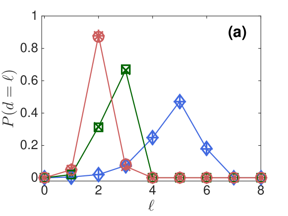
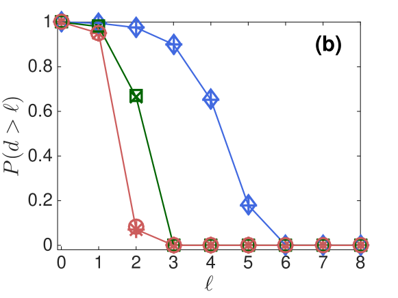
In Fig. 3 we present the DSPL for regular networks of $N=1000$ nodes, with $c=5$, $20$ and $50$, obtained from Eq. (44). The probability distribution function $P(d=\ell)$ is shown in Fig. 3(a) and the tail distribution $P(d>\ell)$ is shown in Fig. 3(b). The results are compared with computer simulations showing excellent agreement.

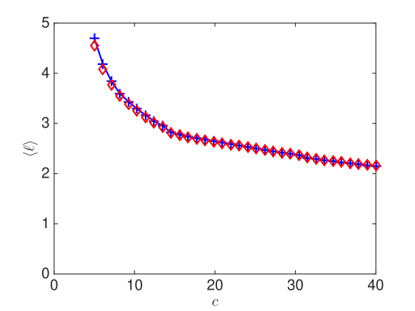
In Fig. 4 we present the mean distance in regular graphs of $N=1000$ nodes vs. the degree $c$, obtained from the recursion equations ($\diamond$). The results are in excellent agreement with numerical simulations ($+$). As expected, the average distance decreases logarithmically as $c$ is increased, in very good agreement with the exact result $\langle\ell\rangle=\ln N/\ln(c-1)$.

For the regular graph, $\langle k\rangle=c$ and $\langle k^{2}\rangle=c^{2}$. Plugging the degenerate degree distribution $p(k)=\delta_{k,c}$ into Eqs. (17) and (18) we obtain that for the regular network $G_{0}(x)=x^{c}$ and $G_{1}(x)=x^{c-1}$. Since the distribution $P_{N}(\ell)$ for the regular network is narrow, one expects the mode $\ell_{\rm mode}$ of this distribution to follow closely the mean value $\langle\ell\rangle$ and to increase logarithmically as a function of $N$. Here we evaluate $\ell_{\rm mode}$ using Eq. (38). Inserting $x_{max}=(c-1)^{-1/(c-1)}$ into Eq. (38) we obtain

$$\ell_{mode}=\frac{\ln N}{\ln(c-1)}+{\cal O}(1).$$ (51)

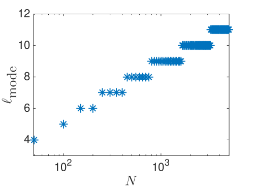
Unlike $\langle\ell\rangle$ the mode takes only integer values. Therefore, it must take the form of a step function vs. $N$. In Fig. 5 we present $\ell_{\rm max}$ vs. $N$ on a semi-logarithmic scale. The general trend indeed satisfies $\ell_{\rm max}\sim\ln N$, but the graph is decorated by steps at integer values of $\ell_{\rm max}$.

V.2 Networks with Binomial Degree Distributions

To further examine the recursion equations, we extend the analysis to networks which exhibit a narrow or bounded degree distribution, with an average $\langle k\rangle=c$ and variance $\sigma_{k}^{2}$. Since the degree distribution, $p(k)$, is a discrete distribution, the binomial distribution

$$p(k)={n\choose k}p^{k}(1-p)^{n-k},$$ (52)

where $n$ is an integer and $0<p<1$, is particularly convenient. Its mean is given by $\langle k\rangle=np$ and its variance is given by $\sigma_{k}^{2}=np(1-p)$. In order to obtain desired values of $\langle k\rangle$ and $\sigma_{k}^{2}$, we choose the parameters $n$ and $p$ according to

$$n={\rm Round}\left(\frac{\langle k\rangle^{2}}{\langle k\rangle-\sigma_{k}^{2}}\right),$$ (53)

where ${\rm Round}(x)$ is the nearest integer to $x$, and

$$p=\frac{\langle k\rangle-\sigma_{k}^{2}}{\langle k\rangle}.$$ (54)

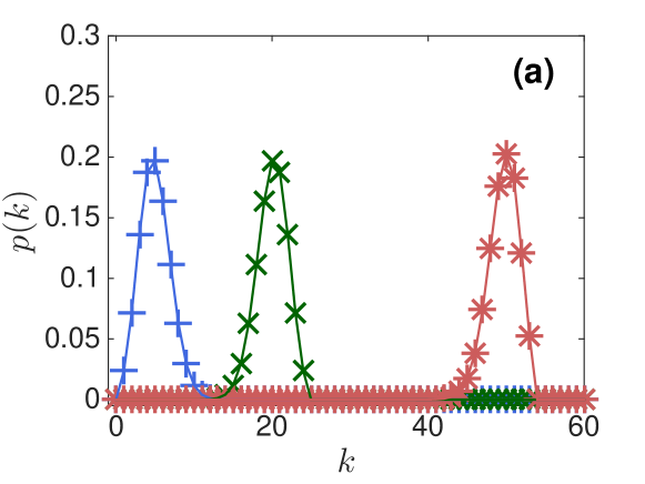
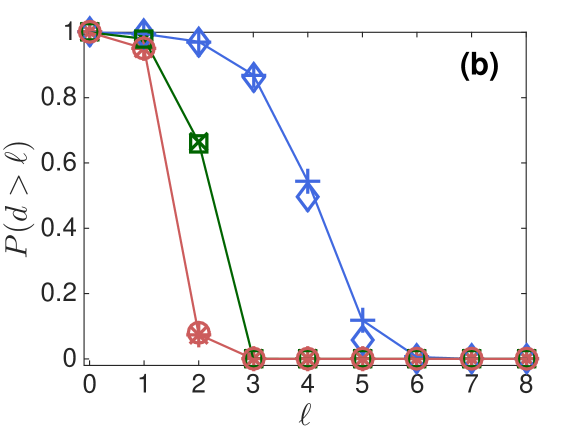
It is important to note that the parameter, $n$, is not related to the network size, $N$, and can be either larger or smaller than $N$. However, one should choose a combination of $n$ and $p$ for which the probability, $p(k)$, for $k>N-1$ is vanishingly small, otherwise a truncation will be needed, which will deform the distribution. In Fig. 6(a) we present the binomial degree distributions of three ensembles of networks of $N=1000$ nodes, $c=5$ (+), $20$ ($\times$) and $50$ ($\ast$) and $\sigma_{k}=4$. In Fig. 6(b) we present the tail distributions $P(d>\ell)$ for these three network ensembles, obtained from the recursion equations for $c=5$ ($\diamond$), $20$ ($\square$) and $50$ ($\circ$). The results are found to be in very good agreement with numerical simulations, (+, $\times$ and $\ast$, respectively), except for the case of $c=5$, where some small deviations are observed. These deviations are due to the fact that in sparse networks the weight of the small, isolated clusters may be non-negligible even above the percolation threshold. This gives rise to some discrepancy between the theoretical and the numerical results for $P(d>\ell)$ for small values of $c$.

Plugging the binomial degree distribution of Eq. (52) into Eqs. (17) and (18) we obtain that $G_{0}(x)=[1-p(1-x)]^{n}$ and $G_{1}(x)=[1-p(1-x)]^{n-1}$. In the asymptotic limit, where $n\gg 1$, this expression converges to $G_{0}(x)\simeq G_{1}(x)\simeq e^{-c(1-x)}$.

Here we evaluate $\ell_{\rm mode}$ for a network with a binomial degree distribution using Eq. (38). For such networks $x_{max}=1-\ln c/c$. Inserting the results above into Eq. (38) we obtain

$$\ell_{mode}=\frac{\ln N}{\ln c}+{\cal O}(1).$$ (55)

Note that Eqs. (51) and (55) differ in their denominators, where the former is $\ln(c-1)$ while the latter is $\ln c$. The reason for this difference comes from the fact that in the regular network each node has exactly $c$ neighbours, and so only $c-1$ of them actually connect inner to outer shells. However, in the binomial case (as in the ER case), each neighbour of the initial node has on average an extra edge, and thus $c$ edges connect an inner shell to an outer shell.

V.3 Networks with Power-Law Degree Distributions

Studies of empirical networks revealed that many of them exhibit power-law degree distributions of the form $p(k)\sim k^{-\gamma}$, where $2<\gamma<3$. This is the range of values of $\gamma$ for which the average degree is bounded but its variance diverges in the infinite system limit. To construct a configuration model network with a power-law distribution $p(k)$, we first choose a lower cutoff $k_{min}\geq 1$ and an upper cutoff $k_{max}\leq N-1$. We then draw the degree sequence $k_{i}$, $i=1,\dots,N$ from the distribution

$$p(k)=Ak^{-\gamma},$$ (56)

where the normalization coefficient is

$$A=[\zeta(\gamma,k_{min})-\zeta(\gamma,k_{max}+1)]^{-1},$$ (57)

and $\zeta(s,a)$ is the Hurwitz zeta function Olver2010 . In the analytical calculations we insert $p(k)$ from Eq. (56) into the recursion equations in order to obtain the distribution of shortest path lengths for the ensemble of networks produced using this degree distribution. In the numerical simulation we repeatedly draw degree sequences from this distribution, produce instances of configuration model networks, calculate the distribution of shortest path lengths in these networks and average over a large number of instances.

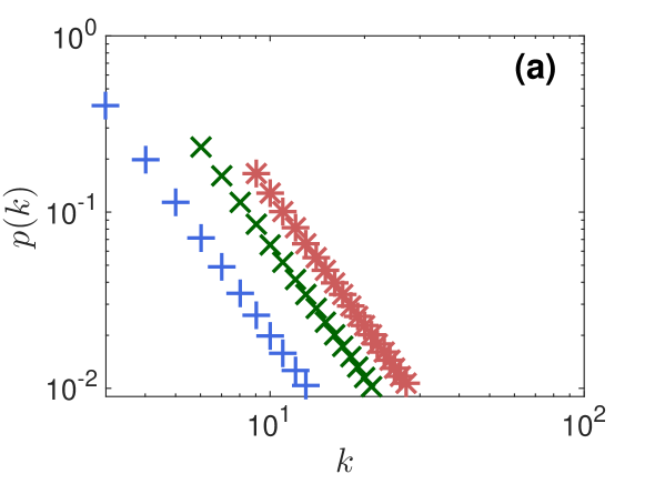
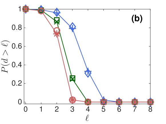
In Fig. 7(a) we present the degree distributions of three scale-free network ensembles with $N=1000$ nodes and $\gamma=2.5$. The lower cutoffs of the degree distributions of these networks are given by $k_{min}=2$, $5$ and $8$, respectively. In each one of these three ensembles, the upper cutoff, $k_{max}$ was chosen such that $p(k_{max})\simeq 0.01$, which means that in a network of 1000 nodes there will be on average about $10$ nodes with degree $k_{max}$. In Fig. 7(b) we present the tail distribution $P(d>\ell)$ for a scale free network with the degree distributions shown in Fig. 7(a). The analytical results are in very good agreement with the numerical simulations.

In the asymptotic limit, where $k_{max}\rightarrow\infty$, the power-law distribution satisfies $\langle k\rangle=\zeta(\gamma-1,k_{min})/\zeta(\gamma,k_{min})$ and $\langle k^{2}\rangle=\zeta(\gamma-2,k_{min})/\zeta(\gamma,k_{min})$. Plugging the power-law degree distribution (56) into Eqs. (17) and (18) we obtain that

$$G_{0}(x)=\frac{\Phi(x,\gamma,k_{min})}{\zeta(\gamma,k_{min})}x^{k_{min}}$$ (58)

and

$$G_{1}(x)=\frac{\Phi(x,\gamma-1,k_{min})}{\zeta(\gamma-1,k_{min})}x^{k_{min}-1},$$ (59)

where $\Phi(x,\gamma,k)$ is the Lerch transcendent Gradshteyn2000 . Evaluating $\ell_{\rm mode}$ for a network with a power-law degree distribution using Eq. (38) we obtain

$$\ell_{mode}=\frac{\ln N}{\ln\left(\frac{\langle k^{2}\rangle-\langle k\rangle}{\langle k\rangle}\right)}+{\cal O}(1).$$ (60)

Note that in scale free networks characterized by $2<\gamma<3$, the value of the second moment $\langle k^{2}\rangle$ is dominated by the upper cutoff, $k_{max}$. As long as $k_{max}$ is kept finite, $\ell_{mode}$ will depend on this upper cutoff. On the other hand, in case that $k_{max}=N-1$, then for $\gamma=3$ one obtains that $(\langle k^{2}\rangle-\langle k\rangle)/\langle k\rangle$ diverges logarithmically with $N$. As a result, $\ell_{mode}\sim\ln N/\ln\ln N$ for large $N$. For $2<\gamma<3$ one obtains that $(\langle k^{2}\rangle-\langle k\rangle)/\langle k\rangle\sim(N-1)^{3-\gamma}$, entailing that $\ell_{mode}={\cal O}(1)$.

The mean distance between nodes in scale free networks was studied in Ref. Cohen2003 . Using an analytical argument it was shown that scale free networks with degree distribution of the form $p(k)\sim k^{-\gamma}$ are ultrasmall, namely exhibit a mean distance which scales like $\langle\ell\rangle\sim\ln\ln N$ for $2<\gamma<3$. For $\gamma=3$ it was shown that the mean distance scales like $\langle\ell\rangle\sim\ln N/\ln\ln N$, while for $\gamma>3$ it coincides with the common scaling of small world networks, namely $\langle\ell\rangle\sim\ln N$. As of now, our approach does not yield a closed form expression for the mean and thus we cannot provide a conclusive result for its scaling with $N$. We do see that the scaling of the mode of the DSPL coincides with the scaling predicted for the mean of the DSPL in Ref. Cohen2003 for $\gamma>3$. In the range $2<\gamma<3$ we find that the mode is of order $1$, namely independent of $N$, which is even shorter than $\ln\ln N$. This is consistent with the ultrasmall scaling of the mean, reported in Ref. Cohen2003 , since the mode is expected to be smaller than the mean and less sensitive to extreme values.

VI Summary and Discussion

We presented a theoretical framework for the calculation of the distributions of shortest path lengths between random pairs of nodes in configuration model networks. This framework, which is based on recursion equations derived using the cavity approach, provides analytical results for the distribution of shortest path lengths. We used the recursion equations to study a broad class of configuration model networks, with degree distributions that follow the degenerate, binomial and power-law distributions. The results were shown to be in good agreement with numerical simulations. The mean, mode and variance of the distribution of shortest path lengths were also evaluated and expressed in terms of moments of the degree distribution, illuminating the important connection between the two distributions. The DSPL is of great relevance to transport processes on networks such as information flow and epidemic spreading. For example, an epidemic tends to spread outwards from the node where it was initiated. As time proceeds, it may reach nodes in shells farther away from the initial node and increases the fraction of infected nodes in the inner shells. Therefore, the number of nodes in each shell and their connectivity affect the rate and efficiency in which the epidemic progresses in the population Shao2015 .

The approach presented in this paper is aimed at the calculation of the entire distribution of distances between pairs of nodes in configuration model networks. In general, it does not provide a closed form expression for the DSPL but a set of recursion equations which can be evaluated for a given network size and a given degree distribution. As a result, it is difficult to obtain a closed form expression for the mean distance, except for special cases such as the regular graph. In fact, for the regular graph, our result for the mean distance coincides with the exact result presented in Ref. Hofstad2005 . Regarding the mode of the DSPL, we do manage to obtain an analytical expression in the general case. The mode turns out to be more amenable to analysis than the mean because it can be determined by a local criterion. For degree distributions with a finite second moment, the mean and the mode tend to scale in a similar fashion. However, in the case of scale free networks, the mean and the mode may scale differently. This is related to the fact that in scale free networks with $2<\gamma<3$, the second moment of the degree distribution, $\langle k^{2}\rangle$, diverges in the infinite system limit. The second moment appears in the equations for the mean distance and for the mode, thus calling for a special care in scale free networks. The mode is less sensitive to extreme values and therefore is expected to be smaller. We find that for $2<\gamma<3$ the mode is of order $1$, namely does not scale with the network size. Lacking a closed form expression for the mean, we cannot provide a conclusive result for the scaling of the mean with the system size. This is an important issue which deserves further research.

M.N. is grateful to the Azrieli Foundation for the award of an Azrieli Fellowship.

Figure 1: (Color online) Illustration of the possible paths of length $\ell$ between two random nodes, $i$ and $j$, in a network of $N$ nodes. The first edge of such a path connects node $i$ to some other node, $r$, which may be any one of the $k$ neighbors of node $i$. The rest of the path, from node $r$ to node $j$ is of length $\ell-1$ and it resides on a smaller network of $N-1$ nodes, from which node $i$ is excluded.

Figure 2: (Color online) Illustration of the iteration process of the recursion equations (19), and (20), which carry over along the diagonals (empty circles). Starting from $\tilde{m}_{N-\ell^{\prime},1}$ (squares), given by Eq. (22), the iteration gives rise to $m_{N,\ell^{\prime}}$ (full circles). Eventually, $P_{N}(d>\ell)$ is obtained as a product of the results in the right-most column [Eq. (23)].

Figure 3: (Color online) Distribution of shortest path lengths in a regular graph. The results of the recursion equations for $P(\ell)$ (a) and $P(d>\ell)$ (b), for $c=5$, $20$ and $50$ ($\Diamond$, $\square$ and $\bigcirc$ , respectively), fit well the numerical results (+, $\times$ and $\ast$, respectively). The numerical results were averaged over $50$ graph instances in a graph of size $N=1000$.

Figure 4: (Color online) Mean shortest path length, $\langle\ell\rangle$, vs. the degree, $c$, in a regular graph of size $N=1000$. The results of the recursion equations ($\Diamond$) are in very good agreement with the numerical results (+). The numerical results were averaged over $50$ graph instances.

Figure 5: (Color online) The mode of the distribution $P_{N}(\ell)$ as a function of the network size, $N$, for a regular network of degree $c=3$. Overall, the mode scales logarithmically with the network size. However, on a finer scale it forms steps due to the discreteness of the distance $\ell$.

Figure 6: (Color online) (a) The degree distributions of three networks of size $N=1000$, where $p(k)$ was drawn from binomial distributions with means $c=5$ , $20$ and $50$ (+, $\times$ and $\ast$, respectively), for which the standard deviation is $\sigma_{k}=4$. The results were obtained from numerical simulations, averaging over $50$ graph instances. These results verify the construction of the configuration model network. (b) The tail distribution $P(d>\ell)$, obtained from the recursion equations ($\Diamond$, $\square$ and $\bigcirc$, respectively), and from numerical simulations (+, $\times$ and $\ast$ , respectively), for the three networks described above. It is observed that as the mean degree is increased, the average distance decreases.

Figure 7: (Color online) (a) The degree distributions of three networks of size $N=1000$, where $p(k)$ was drawn from power-law distributions with $\gamma=2.5$ and lower cutoffs at $k_{min}=2$, $5$ and $8$ (+, $\times$ and $\ast$, respectively). The upper cutoffs, $k_{max}$ were set such that $p(k_{max})=10/N$. The results were obtained from numerical simulations, averaging over $50$ graph instances. (b) The tail distributions $P(d>\ell)$, obtained from the recursion equations ($\Diamond$, $\square$ and $\bigcirc$, respectively), and from numerical simulations (+, $\times$ and $\ast$, respectively), for the three networks described above. It is observed that as the lower cutoff, $k_{min}$, is increased, the mean distance decreases.

References

- (1) R. Albert and A.L. Barabási, Rev. Mod. Phys. 74, 47 (2002).
- (2) G. Caldarelli, Scale free networks: complex webs in nature and technology (Oxford University Press, Oxford, 2007).
- (3) S. Havlin and R. Cohen, Complex Networks: Structure, Robustness and Function (Cambridge University Press, New York, 2010).
- (4) M.E.J. Newman, Networks: an Introduction (Oxford University Press, Oxford, 2010).
- (5) E. Estrada, The structure of complex networks: Theory and applications (Oxford University Press, Oxford, 2011).
- (6) A. Maáyan, S.L. Jenkins, S. Neves, A. Hasseldine, E. Grace, B. Dubin-Thaler, N.J. Eungdamrong, G. Weng, P.T. Ram, J.J. Rice, A. Kershenbaum, G.A. Stolovitzky, R.D. Blitzer, R. Iyengar1, Science 309, 1078 (2005).
- (7) E.W. Dijkstra, Numer. Math. l, 269 (1959).
- (8) D. Delling, P. Sanders, D. Schultes and D. Wagner, Engineering Route Planning Algorithms, in Algorithmics of Large and Complex Networks: Design, Analysis, and Simulation, J. Lerner, D. Wagner, and K.A. Zweig (Eds.), p. 117 (2009).
- (9) I. Abraham, D. Delling, A.V. Goldberg and R.F. Werneck, J. Experimental Algorithmics 18, Article 1.3 (2013).
- (10) R. Pastor-Satorras and A. Vespignani, Phys. Rev. Lett. 86, 3200 (2001).
- (11) R. Pastor-Satorras, C. Castellano, P. Van Mieghem and A. Vespignani, Rev. Mod. Phys. 87, 925 (2015).
- (12) B. Bollobas, Random Graphs, Second Edition (Academic Press, London, 2001).
- (13) D.J. Watts and S.H. Strogatz, Nature 393, 440 (1998).
- (14) A. Fronczak, P. Fronczak, and J.A. Holyst, Phys. Rev. E 70, 056110 (2004).
- (15) M.E.J. Newman, S.H. Strogatz, and D.J. Watts, Phys. Rev. E 64, 026118 (2001).
- (16) V.D. Blondel, J.-L. Guillaume, J.M. Hendrickx and R.M. Jungers, Phys. Rev. E 76, 066101 (2007).
- (17) S.N. Dorogotsev, J.F.F. Mendes and A.N. Samukhin, Nuclear Physics B 653, 307 (2003).
- (18) R. van der Hofstad, G. Hooghiemstra and D. Znamenski, Electronic Journal of Probability 12, 703 (2007).
- (19) R. van der Hofstad and G. Hooghiemstra, J. Math. Phys. 49, 125209 (2008).
- (20) H. van der Esker, R. van der Hofstad and G. Hooghiemstra, J. Stat. Phys. 133, 169 (2008).
- (21) E. Katzav, M. Nitzan, D. ben-Avraham, P.L. Krapivsky, R. Kühn, N. Ross and O. Biham, EPL 111, 26006 (2015).
- (22) P. Erdős and Rényi, Publ. Math. 6, 290 (1959).
- (23) P. Erdős and Rényi, Publ. Math. Inst. Hung. Acad. Sci. 5, 17 (1960).
- (24) P. Erdős and Rényi, Bull. Inst. Int. Stat. 38, 343 (1961).
- (25) M. Molloy and B. Reed, Random Struct. Algorithms 6, 161 (1995).
- (26) Giot et al., Science 302 1727 (2003).
- (27) K.-I. Goh, E. Oh, B. Kahng and D. Kim, Phys. Rev. E 67, 017101 (2003).
- (28) R. Milo, S. Shen-Orr, S. Itzkovitz, N. Kashtan, D. Chklovskii and U. Alon, Science 298, 824 (2002).
- (29) T. Kalisky, R. Cohen, O. Mokryn, D. Dolev, Y. Shavitt and S. Havlin, Phys. Rev. E 74, 066108 (2006).
- (30) J. Shao, S.V. Buldyrev, R. Cohen, M. Kitsak, S. Havlin and H.E. Stanley, EPL 84, 48004 (2008).
- (31) J. Shao, S.V. Buldyrev, L.A. Braunstein, S. Havlin and H.E. Stanley Phys. Rev. E 80, 036105 (2009).
- (32) S. Shao, X. Huang, H.E. Stanley and S. Havlin, New J. Phys. 17, 023049 (2015).
- (33) M. Mézard, G. Parisi and M.A. Virasoro, J. Physique Lett. 46, 217 (1985).
- (34) M. Mézard and G. Parisi, J. Stat. Phys. 111, 1 (2003).
- (35) M. Mézard and A. Montanari, Information, Physics and Computation (Oxford University Press, 2009).
- (36) G. Del Ferraro, C. Wang, D. Martí and M. Mézard, Cavity Method - Message Passing from a Physics Perspective, Statistical Physics, Optimization, Inference and Message-Passing Algorithms, Lecture Notes of the Les Houches School of Physics, Eds. F. Krzakala, F. Ricci-Tersenghi, L. Zdeborova, R. Zecchina, E.W. Tramel, and L.F. Cugliandolo (Oxford University Press, 2015).
- (37) J. Pitman, Probability (Springer, New York, 1993).
- (38) F. Chung and L. Lu, Proc. Nat. Acad. Sci. USA 99, 15879 (2002)
- (39) F. Chung and L. Lu, Internet Mathematics 1, 91 (2004).
- (40) R. van der Hofstad, G. Hooghiemstra and P. Van Mieghem, Random Structures Algorithms 27, 76 (2005).
- (41) H. van den Esker, R. van der Hofstad, G. Hooghiemstra and D. Znamenski, Extremes 8, 111 (2006).
- (42) B. Bollobas, S. Janson and O. Riordan, Random Structures and Algorithms 31, 3 (2007).
- (43) N.C. Wormald, Models of random regular graphs, in LMS Lecture Note Series, Surveys in Combinatorics Eds. J.D. Lamb and D.A. Preece, pages 239-298 (Cambridge University Press, 1999).
- (44) F.W.J. Olver, D.M. Lozier, R.F. Boisvert and C.W. Clark, NIST Handbook of Mathematical Functions (Cambridge University Press, 2010).
- (45) I.S. Gradshteyn and I.M. Ryzhik, Tables of Integrals, Series, and Products, 6th edition (Academic Press, San Diego, 2000).
- (46) R. Cohen and S. Havlin, Phys. Rev. Lett. 90, 058701 (2003).