Propagation of quantum fluctuations in quantum Ising model

Abstract

We investigate the entanglement dynamics between two distant qubits by analyzing correlations in the quantum Ising model. Starting from the spin system in a paramagnetic regime enforced by the external magnetic field $B$, we then switch on the ferromagnetic spin-spin coupling $J$. Using the large coordination number expansion, we consider two limiting switching regimes: (1) adiabatic, which monitors the evolution of the ground state through the quantum transition to an ordered state; and (2) instantaneous (quench) which monitors instead the propagation of quantum fluctuations and simulates the generation of long range correlations. In particular, we find that quantum fluctuations propagate with twice the group speed of excitations in the equilibrium state of the system.

Introduction: The quantum Ising model has recently attracted additional attention as a standard generic model of quantum computers used to evaluate the behaviour of prototype devicesgoogle ; exp2 ; exp3 . In particular, its study would considerably expand our understanding of both fundamental and practical limitations of adiabatic quantum computers and quantum annealers Zagos , where the device is initiated in the strong transverse field, and then the spin-spin (qubit-qubit) coupling is gradually switched on. Entanglement between large number of spins on the intermediate stages of switching plays the key role in the system reaching its final ground state. In a real, open system the adiabatic evolution cannot take an arbitrary long time due to its eventual entanglement with the surroundings Sarandy . The dynamics of entanglement is therefore crucially important for the operation of any quantum annealer.

While the final ground state of a quantum annealer is typically spin-glass like, some insight in this dynamics can be obtained in the simpler case of a sweep through a symmetry-breaking quantum phase transition to the (anti)ferromagnetic order. As the initial quantum state is symmetric, all directions of symmetry breaking are equally likely and seeded by quantum fluctuations. Furthermore, the diverging response time at the critical point indicates that the many-particle quantum system is driven far away from equilibrium during the sweep. While nearby points will most likely break the initial symmetry in the same direction, two very distant points may spontaneously select different directions of symmetry breaking KZ85 . As a result, the spatial order parameter distribution after the quench will be inhomogeneous and its spatial correlations are directly determined by quantum correlations.

The open questions in this context include: How is the order parameter established and how fast does it spread? What is the role of these quantum fluctuations?

In this Letter, we investigate the dynamics of the quantum Ising model both in the case of adiabatic and instantaneous (quench) sweeping with the help of the large coordination-number expansion, which has been previously used mainly in the context of a lattice Bose gas Brout ; NS10 ; NQS14 ; QKNS14 ; KNQS14 . Since this model is only exactly solvable in 1D (one dimension) for nearest-neighbour couplings Pfeuty ; HPK13 , for the Bethe lattice using DMRG NFG08 , or in 2D at the thermal equilibrium Liu , we shall develop an alternative approach capable to handle nonequilibrium dynamics in higher dimension, with the possible applicability to different network connectivity.

After establishing the level of accuracy provided by our approach by comparizon to known exact solutions, we determine the dynamics of quantum fluctuations after a sudden quench to a fixed coupling value and simulate the propagation of correlations inside the qubit system in the process of the ferromagnetic order formation.

Quantum Ising model: We start from the standard Hamiltonian Pfeuty ; NQS14 :

$$\hat{H}=-\frac{J}{Z}\sum_{\mu\nu}T_{\mu\nu}\hat{S}_{\mu}^{z}\hat{S}_{\nu}^{z}-B\sum_{\mu}\hat{S}_{\mu}^{x}\,.$$ (1)

where $\hat{S}_{\mu}^{i}$ ($i=x,y,z$) are spin operators at sites $\mu,\nu$ interacting with each other with a coupling $JT_{\mu\nu}$ and placed in the transverse field $B$. The matrix $T_{\mu\nu}$ encodes the interactions in a $D$-dimensional hypercubic lattice of size $L$ with periodic boundary conditions and is unity only for the nearest neighbours. In that case, the coordination number of the lattice is $Z=2D$. This model displays a quantum transition from the paramagnetic phase (where the transverse magnetic field $B$ dominates) to the ferromagnetic or anti-ferromagnetic phase, which breaks the ${\mathbb{Z}}_{2}$ spin-flip symmetry.

Large coordination number expansion: For $Z\gg 1$, the model dynamics is described using the method developed in NS10 ; QKNS14 . The time evolution of the density matrix $\hat{\rho}$ of the whole lattice is given by the von Neumann-Liouville equation $i\hbar\partial_{t}\hat{\rho}=\left[\hat{H},\hat{\rho}\right]$. This density matrix is usually too complex to be analyzed. Instead the set of reduced density matrices is introduced, $\hat{\rho}_{S}=\,{\rm Tr}_{\not S}\hat{\rho}$, which result from tracing out the Hilbert spaces of all sites except a few: ${\cal S}=\{\mu_{1},\mu_{2},\dots,\mu_{n}\}$. If we keep only one site $\mu$, then the reduced density matrice is a linear operator $\hat{\rho}_{\mu}$ acting on the smaller Hilbert space of one lattice site $\mu$; if we keep two sites $\mu,\nu$, then $\hat{\rho}_{\mu\nu}$ acts on the Hilbert space of two sites etc.

The decomposition $\hat{\rho}_{\mu\nu}=\hat{\rho}_{\mu\nu}^{\rm corr}+\hat{\rho}_{\mu}\hat{\rho}_{\nu}\,,$ and $\hat{\rho}_{\mu\nu\lambda}=\hat{\rho}_{\mu\nu\lambda}^{\rm corr}+\hat{\rho}_{\mu\nu}^{\rm corr}\hat{\rho}_{\lambda}+\hat{\rho}_{\mu\lambda}^{\rm corr}\hat{\rho}_{\nu}+\hat{\rho}_{\nu\lambda}^{\rm corr}\hat{\rho}_{\mu}+\hat{\rho}_{\mu}\hat{\rho}_{\nu}\hat{\rho}_{\lambda}$ etc allows to derive an exact hierarchy of interlinked equations for these operators NS10 ; QKNS14 , the counterpart of the BBGKY chain.

Now we show if the initial state of the system is separable, then the correlations satisfy – at least for a finite period of time – the following hierarchy $\hat{\rho}^{\rm corr}_{\cal S}\sim 1/Z^{|{\cal{S}}|-1}$, that is, the higher-order correlations are suppressed as an inverse power of the coordination number $Z$. More explicitly,

$$\hat{\rho}_{\mu}=\,{\cal O}\left(Z^{0}\right),\,\hat{\rho}^{\rm corr}_{\mu\nu}=\,{\cal O}\left(1/Z\right),\,\hat{\rho}^{\rm corr}_{\mu\nu\kappa}=\,{\cal O}\left(1/Z^{2}\right),$$ (2)

and so on. Using the spin representation, this statement can be rewritten as

$$S^{i}_{\mu}=\langle\hat{S}^{i}_{\mu}\rangle = \,{\cal O}\left(Z^{0}\right),\ \ M_{\mu\nu}^{ij}=\langle\delta\hat{S}^{i}_{\mu}\delta\hat{S}^{j}_{\nu}\rangle=\,{\cal O}\left(1/Z\right),$$

$$\langle\delta\hat{S}^{i}_{\mu}\delta\hat{S}^{j}_{\nu}\delta\hat{S}^{k}_{\kappa}\rangle = \,{\cal O}\left(1/Z^{2}\right),\ \ \dots\quad\quad i,j,k=x,y,z~{},$$ (3)

where $\delta\hat{A}_{\mu}=\hat{A}_{\mu}-\langle\hat{A}_{\mu}\rangle$. THis forms the basis of the $1/Z$-expansion.

Mean-field approach: In the leading order in $1/Z$ we neglect the correlations in order to obtain closed, time-dependent nonlinear mean field equations:

$$\partial_{t}S_{\mu}^{z} = \displaystyle\frac{B}{2}\left(S_{\mu}^{-}-S_{\mu}^{+}\right)\,,$$ (4)

$$i\partial_{t}S_{\mu}^{\pm} = \pm 2J\sum_{\nu}\displaystyle\frac{T_{\mu\nu}}{Z}S_{\mu}^{\pm}S_{\nu}^{z}\mp BS_{\mu}^{z}\,$$ (5)

where $S_{\mu}^{\pm}=S_{\mu}^{x}\pm iS_{\mu}^{y}$. The lowest-order ground state is the mean field solution that minimizes the mean field energy $E_{0}=-B\sum_{\mu}S^{x}_{\mu}-J\sum_{\mu\nu}T_{\mu\nu}S^{z}_{\mu}S^{z}_{\nu}/Z$ with the reduced density matrix corresponding to a pure state $\hat{\rho}^{0}_{\mu}=|\psi\rangle_{\mu}\langle\psi|$ with $|\psi\rangle_{\mu}=c_{\uparrow}|\uparrow\rangle_{\mu}+c_{\downarrow}|\downarrow\rangle_{\mu}$. We find here two regimes separated by a critical point at $J_{c}=B$. For $J<B$, the magnetic field controls the orientation of the spin so that the state is paramagnetic with $S_{\mu}^{z(0)}=0$ and $S_{\mu}^{x(0)}=1/2$ (assuming $B>0$). For $J>B$, on the other hand, we get a non-vanishing ferromagnetic order parameter $S_{\mu}^{z(0)}=\pm\sqrt{1-B^{2}/J^{2}}/2$ (breaking the ${\mathbb{Z}}_{2}$ spin-flip symmetry).

By introducing a linear perturbation around the steady state $S^{i}_{\mu}(t)=S^{i(0)}_{\mu}+S^{i(1)}_{\mathbf{k}}e^{i({\mathbf{k}}.{\mathbf{x}_{\mu}}-\omega_{\mathbf{k}}t)}$, where $\mathbf{x}_{\mu}$ is the site position, we find the excitation modes with the following dispersion relation:

$$\omega_{\mathbf{k}}=\pm\sqrt{4J^{2}\left(S_{\nu}^{z(0)}\right)^{2}+B^{2}-2BJT_{\mathbf{k}}S_{\nu}^{x(0)}}\,.$$ (6)

where we define the Fourier components $T_{\mu\nu}=\frac{1}{L^{D}}\sum_{\mathbf{k}}e^{i\mathbf{k}.(\mathbf{x}_{\mu}-\mathbf{x}_{\nu})}T_{\mathbf{k}}$ whose the expression for nearest neighbours is $T_{\mathbf{k}}=\sum_{i=1}^{D}\cos(k_{i})/D$. In both paramagnetic and ferromagnetic regimes, the spectrum is gapped, but it becomes gapless at the transition. In contrast to this result, in 1D the critical point is at $J_{c}=2B$ Pfeuty . Thus the mean field description valid for large $Z$ displays all essential qualitative features of phase and excitation spectrum but nevertheless appears to be a classical description of the on-site spin vector. Only the next order terms will reflect the quantum fluctuations that form the seeds for the ferromagnetic order.

Adiabatic switching: We start from the initial condition $S_{\mu}^{x}=\frac{1}{2}$, $M_{\mu\nu}^{ij}=0$ which is an eigenstate of an Hamiltonian in absence of ferromagnetism at $J=0$. Then we switch $J(t)$ with some particular time dependence. With such uniform initial conditions, all the spins behave in the same way and the translational invariance imposes correlations depending only on the relative distance so that we define $y(t)=2J(t)S_{\mu}^{i}(t)/B$ and $M_{\mu\nu}^{ij}=\frac{1}{L^{D}}\sum_{\mathbf{k}}e^{i\mathbf{k}.(\mathbf{x}_{\mu}-\mathbf{x}_{\nu})}M^{ij}_{\mathbf{k}}$. The Fourier transform defines also the unphysical uniform correlations, so that the physical correlations are ${\tilde{M}}^{ij}_{\mathbf{k}}=M^{ij}_{\mathbf{k}}-\frac{1}{L^{D}}\sum_{\mathbf{k^{\prime}}}M^{ij}_{\mathbf{k^{\prime}}}$. Using the symmetry $M^{ij}_{\mathbf{k}}=M^{ji}_{\mathbf{k}}$, the non trivial equations of motion are derived from the next order equations of the hierarchyNS10 ; QKNS14 :

$$\partial_{t}\left(\frac{y}{J}\right) = \frac{4J}{BL^{D}}\sum_{\mathbf{k}}T_{\mathbf{k}}M^{yz}_{\mathbf{k}}~{},$$ (7)

$$\partial_{t}M_{\mathbf{k}}^{zz} = -2BM_{\mathbf{k}}^{yz}~{},$$ (8)

$$\partial_{t}M_{\mathbf{k}}^{yz} = -BM_{\mathbf{k}}^{yy}+BM_{\mathbf{k}}^{zz}-BT_{\mathbf{k}}(\tilde{M}^{zz}_{\mathbf{k}}+\frac{1}{4})y~{},$$ (9)

$$\partial_{t}M_{\mathbf{k}}^{yy} = 2BM_{\mathbf{k}}^{yz}-2BT_{\mathbf{k}}\tilde{M}^{yz}_{\mathbf{k}}y~{}.$$ (10)

The ground state solution and quantum transition point are determined by an adiabatic switching with the profile $J(t)=J_{c}\exp(\epsilon t)$ in the interval $t=]-\infty,0]$ with $\epsilon$ infinitesimally small. Noticing that $\partial_{t}=\epsilon J\partial_{J}$, the time parameter is eliminated from the dynamical equations. The introduction of the scaling $M^{yz}_{\mathbf{k}}\rightarrow\epsilon$ and the unity scale for all other dynamical variables together with the elimination of $M^{yz}_{\mathbf{k}}$ using (9) result in the following $\epsilon$-independent equations:

$$\partial_{J}\left(\frac{y}{J}\right) = -\frac{2J}{B^{2}L^{D}}\sum_{\mathbf{k}}T_{\mathbf{k}}\partial_{J}M_{\mathbf{k}}^{zz}~{},$$ (11)

$$M_{\mathbf{k}}^{zz} = M_{\mathbf{k}}^{yy}+T_{\mathbf{k}}(\tilde{M}^{zz}_{\mathbf{k}}+\frac{1}{4})y~{},$$ (12)

$$\partial_{J}M_{\mathbf{k}}^{yy} = -\partial_{J}M_{\mathbf{k}}^{zz}-T_{\mathbf{k}}y\partial_{J}\tilde{M}^{zz}_{\mathbf{k}}~{}.$$ (13)

This independence ensures that the spin system remains in its ground state by tuning $J$, as long as this state is not degenerate. Only at the transition point the excitation spectrum becomes gapless and the smooth evolution is not guaranteed. The elimination of $M^{yy}_{\mathbf{k}}$ from the two last equations leads to a first order equation for $M^{zz}_{\mathbf{k}}$ that is solved using the variable change $y(J)$. We obtain:

$$\tilde{M}_{\mathbf{k}}^{zz}(y)=\frac{1}{\sqrt{1-yT_{\mathbf{k}}}}\left[\frac{1}{4}-\int_{0}^{y}\!\!\!\!\!dy^{\prime}\frac{\partial_{y^{\prime}}f_{0}(y^{\prime})}{\sqrt{1-y^{\prime}T_{\mathbf{k}}}}\right]-\frac{1}{4}$$ (14)

where $f_{0}=L^{-D}\sum_{\mathbf{k^{\prime}}}M^{zz}_{\mathbf{k^{\prime}}}$. The application of the condition $L^{-D}\sum_{\mathbf{k}}\tilde{M}^{zz}_{\mathbf{k}}=0$ to this last equation provides a one-dimensional closed integral equation for $f_{0}(y)$:

$$\frac{1}{L^{D}}\sum_{\mathbf{k}}\frac{1}{\sqrt{1-yT_{\mathbf{k}}}}\left[1-\int_{0}^{y}\!\!\!\!\!dy^{\prime}\frac{4\partial_{y^{\prime}}f_{0}(y^{\prime})}{\sqrt{1-y^{\prime}T_{\mathbf{k}}}}\right]=1~{}.$$ (15)

Together with Eq.(11), they provide the spin solution with a low cost in terms of computation time through integration:

$$S^{x}_{\mu}(y)=\left[\frac{1}{4}-\int_{0}^{y}\!\!\!\!\!dy^{\prime}y^{\prime}\frac{1}{L^{D}}\sum_{\mathbf{k}}T_{\mathbf{k}}\partial_{y^{\prime}}{\tilde{M}}^{zz}_{\mathbf{k}}(y^{\prime})\right]^{1/2}.$$ (16)

The singularity appearing at $y(J)=1$ corresponds to the quantum phase transition at $({S^{x}}_{\mu})_{c}=(B/2J)_{c}$ up to the next order in $1/Z$. In that case the correlations become singular at $\mathbf{k}=0$. For nearest neighbour interactions, we obtain the long wavelength scaling $\tilde{M}_{\mathbf{k}}^{zz}(y=1)\rightarrow 1/|\mathbf{k}|$.

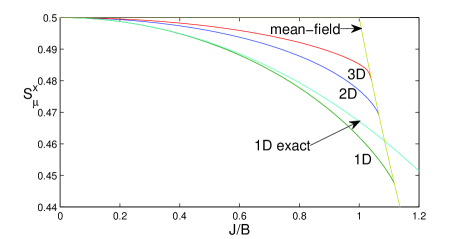
The results are plotted in Fig.1 for the large system size ($L\rightarrow\infty$) and go beyond the mean-field results. For $D=1$, there exist an analytical solution, and the next-order correction already converges quite well to the exact value, with the critical point given by:

$$({S^{x}_{\mu}})_{c}=\sqrt{\frac{\sqrt{2}}{\pi}-\frac{1}{4}}\simeq 0.44~{}.$$ (17)

This value is closer to the exact one $(S^{x}_{\mu})_{c}=1/\pi=0.32$ in Pfeuty and shofts the critical coupling in the right direction, to $(J/B)_{c}=1.12$, which is nevertheless still below the exact value of $(J/B)_{c}=2$. For $D=2$, the critical value $(J/B)_{c}=1.075$ approaches better the exact result $(J/B)_{c}=1.314$ obtained through the quantum Monte-Carlo method Liu . For $D=3$ the obtained value $(J/B)_{c}=1.042$ is even closer to the mean field curve. It is reasonable to expect it to better fit the exact results for larger coordination number.

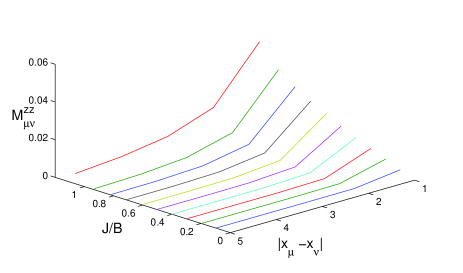
We note that the transition takes place once the spin value reaches the mean field value in the ferromagnetic regime. The spin reduction is a signature of the global entanglement of a given site with all the others which can be estimated through the relation $\eta_{\mu}=2\left[1-\,{\rm Tr}(\hat{\rho}_{\mu}^{2})\right]=1-4{S^{x}_{\mu}}^{2}$. It shows that the entanglement increases close to the transition point but decreases with the dimensionality of the system. The Fig.2 displays the growing extension of the range of quantum fluctuations as we approach the transition at which all sites becomes correlated.

Generally, all the results obtained by adding the two-sites correlations improve over the mean-field approach and reproduce correctly the physical properties of the ground state, especially in higher dimensions.

Figure 1: Plot of the spin $S^{x}_{\mu}$ vs. $J/B$ in $D=1,2$ and $3$. The mean-field and 1D exact results are plotted for comparison.

Figure 2: Plots of the quantum fluctuations correlator $M^{zz}_{\mu\nu}$ vs. $J/B$ and intersite distances $|{\bf x}_{\mu}-{\bf x}_{\nu}|$ in 2D ($L=40$).

Quench dynamics: Now we use our approach to describe the dynamics of quenching. We start from $J=0$ and we instantanously switch it to a final value $J$. On the time scale much shorter than the decoherence time, the evolution of the spin system can be considered as entirely determinist when starting from the zero temperature ground state. Therefore any fluctuations resulting from the quench are purely quantum over this time interval.

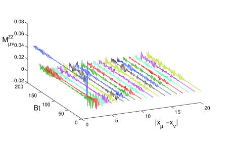
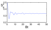
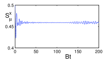
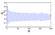
In the paramagnetic regime ($J<J_{c}$), the transverse spin evolves to reach a steady value lower than the corresponding one for the ground state but still close to $1/2$. We observe a wave pulse-like generation of the correlations that propagate just after the quench. The propagation speed is constant and estimated as $twice$ the group velocity Eq.(6) of the excitation in the system, $c={\rm Max}\left(2\partial\omega_{\mathbf{k}}/\partial k_{x}\right)=2(J/Z)[{1-J(Z-2)/(BZ)}]^{-1/2}$. The factor two corresponds to spontaneous virtual excitations always created in pairs and follows from the physical reality that at least two kinks are needed for a spin domain formation. In the case of $J/B=0.8$ in Fig.3, we obtain the value $c\simeq 0.5B$. In a system with periodic boundary condition, the signal is reflected back as an echo that affects the transverse spin at $Bt=150$ with a small oscillating burst. The amplitude of the pulse is modulated by oscillations of frequency estimated as $2B\sqrt{1-J/B}/2\pi$. As a result of random waves, the correlations remain short-ranged and the total magnetization fluctuations $M^{zz}={\tilde{M}}_{\mathbf{k}=0}^{zz}$ along the $z$ axis cannot develop but instead stay confined to a small value as can be seen in the second graph of Fig.3.

The visible wavefront can be exploited to test the quantum character of the interaction between the spin sites. It is an essentially quantum prediction, which goes beyond the mean-field approach.

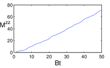
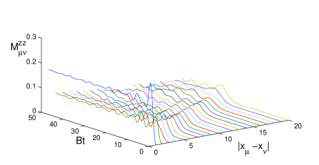
In the case of a quench beyond the critical value, $J>J_{c}$, the sweep is done in the ferromagnetic region and quantum correlations develop over a long range. The frequency of propagation becomes imaginary and leads to an exponential increase with a rate given by $\gamma=2\omega_{\mathbf{k}=0}/i=2B\sqrt{2JS_{\mu}^{x}/B-1}\sim(J-J_{c})^{1/2}$. The second graph of Fig.4 shows indeed a growing $M^{zz}=M^{zz}_{max}\gamma t$ for $J/B=1.5$, where $M^{zz}_{max}=L^{D}/4$ corresponds to the maximum possible value of the fluctuations correlator, while the average spin stabilizes to a much lower steady state value. Using the long-wavelength approximation $2\omega_{\mathbf{k}=0}=i\sqrt{\gamma^{2}-v^{2}{\mathbf{k}}^{2}}$ where $v=2JS_{\mu}^{x}B$, the saddle point method is used to estimate the scaling of the onset of correlations NS10 :

$${M}^{zz}_{\mu\nu}\sim\exp(\gamma\sqrt{t^{2}-|{\mathbf{x}}_{\mu}-{\mathbf{x}}_{\nu}|^{2}/v^{2}})~{}.$$ (18)

This dominant term displays a finite propagation speed $v$ for the onset of correlations shown in Fig.4. It tells about the pre-stage dynamics towards a steady ferromagnetic state. Nevertheless, this analysis is restricted to a short time scale within the region of the instability of the growing modes and thus cannot be extended to study the evolution towards the thermodynamic equilibrium.

Figure 3: Quench dynamics: time evolution of spin $S^{x}_{\mu}$, the fluctuation correlator $M^{zz}_{\bf k=0}$ and local fluctuation correlators $M_{\mu\nu}^{zz}$ along the principal axis for $J/B=0.8$ in 2D ($L=40$).

Figure 4: Same as in Fig.3 but for $J/B=1.5$.

In summary: We have used the large coordination number expansion developed in NS10 ; QKNS14 in order to describe the nonequilibrium dynamics of the quantum Ising model. Since this technique is based on the evolution equations of reduced density matrices, it can be used efficently for numerical simulations. The lowest order in $1/Z$ reproduces the mean-field classical approach; the higher orders describe quantum correlations. This method has been applied to calculate the creation and amplification of quantum correlations in a quenched paramagnetic-ferromagnetic phase transition. We find that the off-site long-range order spreads with a constant velocity exceeding the excitation speed in the system in equilibrium. An experimental observation of this effect could provide arguments in favour of quantum dynamics of an artificial quantum structure such as a quantum annealer.

References

• (1) V.S. Denchev, S. Boixo, S.V. Isakov, N. Ding, R. Babbush, V. Smelyanskiy, J. Martinis, and H. Neven, arXiv:1512.02206.
• (2) T. F. Rรธnnow, Z. Wang, J. Job, S. Boixo, S. V. Isakov, D. Wecker, J. M. Martinis, D. A. Lidar, M. Troyer, Science 345, 420 (2014)
• (3) S. Boixo, T. F. Rรธnnow, S. V. Isakov, Z. Wang, D. Wecker, D. A. Lidar, J. M. Martinis, M. Troyer, Nature Phys. 10, 218 (2014).
• (4) A.M. Zagoskin, E. Ilโ€™ichev, M. Grajcar, J.J. Betouras, and F. Nori, Front. in Physics 2: 33 (2014).
• (5) M. S. Sarandy and D. A. Lidar, Phys. Rev. Lett. 95, 250503 (2005).
• (6) T.W. B. Kibble, J. Phys. A 9, 1387 (1976);W. H. Zurek, Nature (London) 317, 505 (1985).
• (7) R.ย Brout, Phys.ย Rev.ย A 118, 1009 (1960); R.ย  Brout, Phys.ย Rev.ย A115, 824 (1959); R.B. Stinchcombe, J. Phys. C 6, 2459 (1973); R.B. Stinchcombe, J. Phys. C 6, 2484 (1973).
• (8) P.ย Navez and R.ย Schรผtzhold, Phys.ย Rev.ย A 82, 063603 (2010); F. Queisser, P. Navez and R. Schรผtzhold J. Phys.: Condens. Matter 25, 404215 (2013).
• (9) P. Navez, F. Queisser, R. Schรผtzhold, J. Phys. A: Math. Theor. 47, 225004 (2014).
• (10) F. Queisser, K. V. Krutitsky, P. Navez, R. Schรผtzhold, Phys.ย Rev.ย A 89, 033616 (2014).
• (11) K.V. Krutitsky, P. Navez, F. Queisser, R. Schรผtzhold EPJ Quantum Technology 1:12 (2014).
• (12) P. Pfeuty, Ann. Phys. 57, 79-90 (1970).
• (13) C.-W. Liu, A. Polkovnikov, and A. W. Sandvik, Phys.ย Rev.ย B 87, 174302 (2013).
• (14) D. Nagaj, E. Farhi, J. Goldstone, P. Shor, and I. Sylvester Phys. Rev. B 77, 214431 (2008).
• (15) M. Heyl, A. Polkovnikov, and S. Kehrein Phys. Rev. Lett. 110, 135704 (2013).