A posteriori error estimates for discontinuous Galerkin methods using non-polynomial basis functions.
Part II: Eigenvalue problems

Abstract.

We present the first systematic work for deriving a posteriori error estimates for general non-polynomial basis functions in an interior penalty discontinuous Galerkin (DG) formulation for solving eigenvalue problems associated with second order linear operators. Eigenvalue problems of such types play important roles in scientific and engineering applications, particularly in theoretical chemistry, solid state physics and material science. Based on the framework developed in [L. Lin, B. Stamm, http://dx.doi.org/10.1051/m2an/2015069] for second order PDEs, we develop residual type upper and lower bound error estimates for measuring the a posteriori error for eigenvalue problems. The main merit of our method is that the method is parameter-free, in the sense that all but one solution-dependent constants appearing in the upper and lower bound estimates are explicitly computable by solving local and independent eigenvalue problems, and the only non-computable constant can be reasonably approximated by a computable one without affecting the overall effectiveness of the estimates in practice. Compared to the PDE case, we find that a posteriori error estimators for eigenvalue problems must neglect certain terms, which involves explicitly the exact eigenvalues or eigenfunctions that are not accessible in numerical simulations. We define such terms carefully, and justify numerically that the neglected terms are indeed numerically high order terms compared to the computable estimators. Numerical results for a variety of problems in 1D and 2D demonstrate that both the upper bound and lower bound are effective for measuring the error of eigenvalues and eigenfunctions.

1. Introduction

Let $\Omega$ be a rectangular, bounded domain. We consider the following linear eigenvalue problem of finding an eigenvalue $\lambda$ and the corresponding eigenfunction $u$, with $\|u\|_{\Omega}=1$, such that

$$-\Delta u+Vu=\lambda u,\qquad\mbox{in }\Omega,$$ (1)

where $V$ is a bounded, smooth potential. Such eigenvalue problem arises in many scientific and engineering problems. One notable example is the Kohn-Sham density functional theory [27], which is widely used in theoretical chemistry, solid state physics and material science. In order to solve Eq. (1) in practice, it is desirable to reduce the number of degrees of freedom for discretizing Eq. (1) to have a smaller algebraic problem to solve. While standard polynomial basis functions and piecewise polynomial basis functions can approach a complete basis set and is versatile enough to represent almost any function of interest, the resulting number of degrees of freedom is usually large even when high order polynomials are used. Non-polynomial basis functions are therefore often employed to reduce the number of degrees of freedom. Examples include the various non-polynomial basis sets used in quantum chemistry such as the Gaussian basis set [14], atomic orbital basis set [24], adaptive local basis set [32], planewave discretization [5]. Similar techniques also appear in other contexts, such as the planewave basis set for solving the eigenvalue problems in photonic crystals [23], Helmholtz equations [19, 41], and heterogeneous multiscale method (HMM) [11] and the multiscale finite element method [20] for solving multiscale elliptic equations.

1.1. Previous work on a posteriori estimates

Concerning the Laplace eigenvalue problem (Eq. (1) with $V=0$), there has been important progress in particular in obtaining guaranteed lower bounds for the first eigenvalue using polynomial-based versions of the finite element method: Armentano and Durán [1], Hu et al. [21, 22], Carstensen and Gedicke [8], and Yang et al. [44] achieve so via the lowest-order nonconforming finite element method. Kuznetsov and Repin [30], and Šebestová and Vejchodský [39] give numerical-method-independent estimates based on flux (functional) estimates, and Liu and Oishi [34] elaborate a priori approximation estimates for lowest-order conforming finite elements. Cancès et al. [7] present guaranteed bounds for the eigenvalue error for the classical conforming finite element method. A posteriori estimates for the polynomial $hp$-discontinuous Galerkin (DG) method are developed by Giani and Hall [15]. Earlier work comprises Kato [25], Forsythe [12], Weinberger [43], Bazley and Fox [3], Fox and Rheinboldt [13], Moler and Payne [36], Kuttler and Sigillito [28, 29], Still [40], Goerisch and He [16], and Plum [37].

The question of accuracy for both eigenvalues and eigenvectors has also been investigated previously. For conforming finite elements, relying on the a priori error estimates resumed in Babuška and Osborn [2], Boffi [4] and references therein, a posteriori error estimates have been obtained by Verfürth [42], Maday and Patera [35], Larson [31], Heuveline and Rannacher [18], Durán et al. [9], Grubišić and Ovall [17], Rannacher et al. [38], and Cancès et al. [7].

For non-polynomial basis functions, the literature is much sparser. A posteriori estimates for planewave discretization of non-linear Schrödinger eigenvalue problems are presented in Dusson and Maday [10], and Cancès et al. [6]. Kaye et al. [26] developed upper bound error estimates for solving linear eigenvalue problems using non-polynomial basis functions in a DG framework, which generalizes the work of Giani et al. [15] for polynomial basis functions.

1.2. Contribution

We present a systematic way of deriving residual-based a posteriori error estimates for the discontinuous Galerkin (DG) discretization of problem (1) using non-polynomial basis functions. More precisely, we derive computable upper and lower bounds for both the error of eigenvalues and eigenvectors, up to some terms that are asymptotically of higher order. This extends the framework introduced in the companion paper [33] on second order PDEs. The main difficulty can be reduced to the non-existence of inverse estimates for arbitrary non-polynomial basis functions and the non-existence of an accurate conforming subspace. In the present approach, all but one basis-dependent constant appearing in the upper and lower bound estimates are explicitly computable by solving local eigenvalue problems. For solutions with sufficient regularity (for instance $u\in H^{2}(\Omega)$), the only non-computable constant can be reasonably approximated by a computable one without affecting the overall effectiveness of the estimates. While the requirement of $H^{2}(\Omega)$ regularity appears to be a formal drawback in the context of a posteriori error estimates, the main goal of this work is to develop a posteriori error estimates for general basis sets rather than for $h$-refinement, and the difficulty of general basis sets holds even if the solution has $C^{\infty}(\Omega)$ regularity. Therefore we think our method can have important practical values.

Our estimators for eigenfunctions are very similar to those for second order PDEs, and our estimators for eigenvalues are derived from the eigenfunction estimators. By leveraging the same constant related to the regularity of the eigenfunction $u\in H^{2}(\Omega)$, we arrive at simpler treatment for upper and lower estimators for eigenvalues. Compared to the treatment in literature [15], our treatment does not involve the usage of lifting operators. Compared to the PDE case, we find that a posteriori error estimators for eigenvalue problems must neglect certain terms, which involve explicitly the exact eigenvalues and eigenfunctions that are not accessible in numerical simulation. We define such terms carefully, and justify numerically that the neglected terms are indeed high order terms compared to the computable estimators. Our numerical results in 1D and 2D illustrate the effectiveness of the estimators.

1.3. Outline

We introduce in Section 2 preliminary results that are needed to introduce the discontinuous Galerkin discretization of the eigenvalue problem (1) and the following a posteriori analysis that are both presented in Section 3. Section 4 is devoted to numerical tests, followed by the conclusion in Section 5.

2. Preliminary results

2.1. Mesh, broken spaces, jump and average operators

Let $\Omega=(0,1)^{d}$, $d=1,2,3$ and let ${\mathcal{K}}$ be a regular partition of $\Omega$ into elements $\kappa\in{\mathcal{K}}$. That is, we assume that the interior of $\overline{\kappa}\cap\overline{\kappa}^{\prime}$, for any $\kappa,\kappa^{\prime}\in{\mathcal{K}}$, is either an element of ${\mathcal{K}}$, a common face, edge, vertex of the partition or the empty set. For simplicity, we identify the boundary of $\Omega$ in a periodical manner. That means, that we also assume the partition to be regular across the boundary $\partial\Omega$. We remark that although the assumption of a rectangular domain with periodic boundary condition appears to be restrictive, such setup already directly finds its application in important areas such as quantum chemistry and materials science. However, the analysis below is not restricted to equations with periodic boundary condition. Other boundary conditions, such as Dirichlet or Neumann boundary conditions can be employed as well with minor modification. Generalization to non-rectangular domain does not introduce conceptual difficulties either, but may lead to changes in numerical schemes for estimating relevant constants, if the tensorial structure of the grid points is not preserved.

Let $N=(N_{\kappa})_{\kappa\in{\mathcal{K}}}$ denote the vector of the local number of degrees of freedom $N_{\kappa}$ on each element $\kappa\in{\mathcal{K}}$. Let $\mathbb{V}_{N}=\bigoplus_{\kappa\in{\mathcal{K}}}\mathbb{V}_{N}(\kappa)$ by any piecewise discontinuous approximation space on a partition ${\mathcal{K}}$ of the domain $\Omega$. It is important to highlight that little is assumed about the a priori information of $\mathbb{V}_{N}$ except that we assume that each $\mathbb{V}_{N}(\kappa)$ contains constant functions and that $\mathbb{V}_{N}(\kappa)\subset H^{\frac{3}{2}}(\kappa)$, so that the traces of $\nabla v_{N}$ on the boundary $\partial\kappa$ are well-defined for all $v_{N}\in\mathbb{V}_{N}(\kappa)$, for all $\kappa\in{\mathcal{K}}$.

We denote by $H^{s}(\kappa)$ the standard Sobolev space of $L^{2}(\kappa)$-functions such that all partial derivatives of order $s\in\mathbb{N}$ or less lie as well in $L^{2}(\kappa)$. By $H^{s}({\mathcal{K}})$, we denote the set of piecewise $H^{s}$-functions defined by

$$H^{s}({\mathcal{K}})=\left\{v\in L^{2}(\Omega)\,\middle|\,v|_{\kappa}\in H^{s}(\kappa),\forall\kappa\in{\mathcal{K}}\right\},$$

also referred to as the broken Sobolev space. We denote by $H^{1}_{\#}(\Omega)$ the space of periodic $H^{1}$-functions on $\Omega$. We further define the element-wise resp. face-wise scalar-products and norms as

$$(v,w)_{\mathcal{K}}=\sum_{\kappa\in{\mathcal{K}}}(v,w)_{\kappa}\qquad\mbox{and}\qquad\|v\|_{\mathcal{K}}=(v,v)_{\mathcal{K}}^{\frac{1}{2}}.$$

The $L^{2}$-norm on $\kappa$ and $\Omega$ are denoted by $\|\cdot\|_{\kappa}$ and $\|\cdot\|_{\Omega}$, respectively. The jump and average operators on a face $\overline{F}=\overline{\kappa}\cap\overline{\kappa}^{\prime}$ are defined in a standard manner by

$$\{\{v\}\}=\tfrac{1}{2}(v|_{\kappa}+v|_{\kappa^{\prime}}),\qquad \mbox{and}\qquad\qquad[\![v]\!]=v|_{\kappa}n_{\kappa}+v|_{\kappa^{\prime}}n_{\kappa^{\prime}},$$

$$\{\{\nabla v\}\}=\tfrac{1}{2}(\nabla v|_{\kappa}+\nabla v|_{\kappa^{\prime}}),\qquad \mbox{and}\qquad\qquad[\![\nabla v]\!]=\nabla v|_{\kappa}\cdot n_{\kappa}+\nabla v|_{\kappa^{\prime}}\cdot n_{\kappa^{\prime}},$$

where $n_{\kappa}$ denotes the exterior unit normal of the element $\kappa$. Finally we recall the standard result of piecewise integration by parts formula that will be employed several times in the upcoming analysis.

Lemma 2.1.

Let $v,w\in H^{2}({\mathcal{K}})$. Then, there holds

$$\sum_{\kappa\in{\mathcal{K}}}\Big{[}(\Delta v,w)_{\kappa}+(\nabla v,\nabla w)_{\kappa}\Big{]}=\tfrac{1}{2}\sum_{\kappa\in{\mathcal{K}}}\Big{[}([\![\nabla v]\!],w)_{\partial\kappa}+(\nabla v,[\![w]\!])_{\partial\kappa}\Big{]}.$$

2.2. Projections

For any element $\kappa\in{\mathcal{K}}$, let us denote by $\Pi^{\kappa}_{0}:L^{2}(\kappa)\to\mathbb{R}$ the $L^{2}(\kappa)$-projection onto constant functions defined by

$$(\Pi^{\kappa}_{0}v,w)_{\kappa}=(v,w)_{\kappa},\qquad\forall w\in\mathbb{R},$$

that is explicitly given by $\Pi^{\kappa}_{0}v=\frac{1}{|\kappa|}\int_{\kappa}v\,dx$. On $H^{1}(\kappa)$ we define the following scalar product and norm

$$(v,w)_{\star,\kappa} =(\Pi^{\kappa}_{0}v,\Pi^{\kappa}_{0}w)_{\kappa}+(\nabla v,\nabla w)_{\kappa},$$ (2)

$$\|v\|_{\star,\kappa} =(v,v)_{\star,\kappa}^{\frac{1}{2}},$$

for all $v,w\in H^{1}(\kappa)$ and the corresponding projection $\Pi_{N}^{\kappa}:H^{1}(\kappa)\to\mathbb{V}_{N}(\kappa)$ by

$$(\Pi_{N}^{\kappa}v,w_{N})_{\star,\kappa}=(v,w_{N})_{\star,\kappa}\qquad\forall w_{N}\in\mathbb{V}_{N}(\kappa).$$ (3)

Then, it is easy to see that this projection satisfies the following properties

$$(v-\Pi_{N}^{\kappa}v,c)_{\kappa} =0, \forall c\in\mathbb{R},\forall v\in H^{1}(\kappa),$$

or equivalently expressed as $\Pi^{\kappa}_{0}(v-\Pi_{N}^{\kappa}v)=0$. This implies that

$$(\nabla(v-\Pi_{N}^{\kappa}v),\nabla w_{N})_{\kappa} =0, \forall w_{N}\in\mathbb{V}_{N}(\kappa),\forall v\in H^{1}(\kappa),$$ (4)

$$\|\nabla(v-\Pi_{N}^{\kappa}v)\|_{\kappa} \leq\|\nabla v\|_{\kappa}, \forall v\in H^{1}(\kappa),$$ (5)

$$\|v-\Pi_{N}^{\kappa}v\|_{\star,\kappa} \leq\|v\|_{\star,\kappa}, \forall v\in H^{1}(\kappa).$$

2.3. Local scaling constants

In this section, we recall some local constants that will be used in the upcoming a posteriori error analysis and that were introduced in [33]. We start with recalling the local trace inverse inequality constant ${\tt d}_{\kappa}$ for each $\kappa\in{\mathcal{K}}$ defined by

$${\tt d}_{\kappa}\equiv\sup_{v_{N}\in\mathbb{V}_{N}(\kappa)}\frac{\|\nabla v_{N}\cdot n_{\kappa}\|_{\partial\kappa}}{\|v_{N}\|_{\star,\kappa}}>0.$$

Further, we consider

$${\tt a}_{\kappa}\equiv\sup_{\begin{subarray}{c}v\in H^{1}(\kappa),\\ v\perp\mathbb{V}_{N}(\kappa)\end{subarray}}\frac{\|v\|_{\kappa}}{\|v\|_{\star,\kappa}}\qquad\mbox{and}\qquad{\tt b}_{\kappa}\equiv\sup_{\begin{subarray}{c}v\in H^{1}(\kappa),\\ v\perp\mathbb{V}_{N}(\kappa)\end{subarray}}\frac{\|v\|_{\partial\kappa}}{\|v\|_{\star,\kappa}},$$

where $\perp$ is in the sense of the scalar product $(\cdot,\cdot)_{\star,\kappa}$ defined by (2).

Remark 2.2 (The computation of the constants ${\tt a}_{\kappa}$, ${\tt b}_{\kappa}$ and ${\tt d}_{\kappa}$).

More details on how these local constants can be approximated by solving local eigenvalue problems is explained in detail in [33, Section 5]

3. Eigenvalue problem

We first assume that the smallest eigenvalue $\lambda\in\mathbb{R}$ is non-degenerate. Consider the problem of finding this smallest eigenvalue $\lambda$ and the corresponding eigenfunction $u\in H^{1}_{\#}(\Omega)\cap H^{2}({\mathcal{K}})$ with $\|u\|_{\Omega}=1$ such that

$$-\Delta u+Vu=\lambda u,\quad\mbox{in }\Omega.$$ (6)

We assume that $V$ is bounded and smooth. Observing that adding any constant to the potential results in a modified eigenvalue which is shifted by the same value, we can assume that $V$ is positive. The choice of the constant only affects the high order terms that is absent in the leading computable upper and lower bound estimators.

For some $\theta\in\mathbb{R}$ and $\gamma:\Omega\to\mathbb{R}$ such that $\gamma|_{\kappa}=\gamma_{\kappa}\in\mathbb{R}$ and using the bilinear form

$$a(w,v) =\sum_{\kappa\in{\mathcal{K}}}\Big{[}(\nabla w,\nabla v)_{\kappa}+(Vw,v)_{\kappa}\Big{]}+\tfrac{1}{2}\sum_{\kappa\in{\mathcal{K}}}\Big{[}-(\nabla w,[\![v]\!])_{\partial\kappa}-\theta([\![w]\!],\nabla v)_{\partial\kappa}+\gamma_{\kappa}([\![w]\!],[\![v]\!])_{\partial\kappa}\Big{]},$$

the approximated eigenvalue problem can be stated as: Find the smallest, non-degenerate eigenvalue $\lambda_{N}\in\mathbb{R}$ and $u_{N}\in\mathbb{V}_{N}$ with $\|u_{N}\|_{\Omega}=1$ such that

$$a(u_{N},v_{N})=\lambda_{N}(u_{N},v_{N})_{\Omega},\qquad\forall v_{N}\in\mathbb{V}_{N}.$$ (7)

In order to quantify the error, we introduce the broken energy norm

$$|\!|\!|v|\!|\!|^{2}=\sum_{\kappa\in{\mathcal{K}}}\Big{[}\|\nabla v\|_{\kappa}^{2}+\tfrac{\gamma_{\kappa}}{2}\|[\![v]\!]\|_{\partial\kappa}^{2}+\|V^{\frac{1}{2}}v\|^{2}_{\kappa}\Big{]},\quad\forall v\in H^{1}({\mathcal{K}}).$$

As usual, the penalty parameter $\gamma$ needs to be chosen sufficiently large to ensure coercivity of the bilinear form, and the energy norm error for eigenfunctions is defined to be $|\!|\!|u-u_{N}|\!|\!|$.

Following the technique introduced in [33] we obtain the following result.

Lemma 3.1.

If $\gamma_{\kappa}\geq\frac{1}{2}\,(1+\theta)^{2}\,({\tt d}_{\kappa})^{2}$, then the bilinear form is coercive on $\mathbb{V}_{N}$, i.e., there holds

$$\tfrac{1}{2}|\!|\!|v_{N}|\!|\!|^{2}\leq a(v_{N},v_{N}),\qquad\forall v_{N}\in\mathbb{V}_{N}.$$

Proof.

The proof is basically identical with the one presented in [33, Lemma 3.1]. The only slight difference is that the broken energy norm as well as the bilinear form have now the positive contribution $\|V^{\frac{1}{2}}v_{N}\|^{2}_{\kappa}$. ∎

Remarkably, this lemma provides a computable and sharp value for each $\gamma_{\kappa}$ such that the bilinear form is coercive.

Remark 3.2.

Note that even when the smallest eigenvalue $\lambda_{N}$ is a non-degenerate eigenvalue, the corresponding eigenfunction $u_{N}$ still has an arbitrary phase factor $\pm 1$. If such phase factors from $u$ and $u_{N}$ do not match, the error $u-u_{N}$ must be of order $1$. Since $u-u_{N}$ never appears in the upper or lower bound estimators, such phase factors will not affect the computation of the estimators, and only arise when comparing the estimators with the true error $|\!|\!|u-u_{N}|\!|\!|$. In such case, the phase factor can be eliminated by a “subspace alignment” procedure to be discussed in section 4. The same procedure can be applied to align eigenfunctions when more eigenvalues and eigenfunctions are to be computed, even when some of the eigenvalues are degenerate. Below we assume that $u$ and $u_{N}$ are aligned eigenfunctions so that the error $|\!|\!|u-u_{N}|\!|\!|$ converges to $0$ as the basis function refines.

3.1. A posteriori estimates of eigenfunctions

We adapt here the residual type estimators obtained in [33] to the case of eigenvalue problems.

3.1.1. Error representation

Recall that we assumed that $u\in H^{2}(\kappa)$, we introduce the constant ${\tt d}_{\kappa}^{u}(u_{N})$ defined by

$${\tt d}_{\kappa}^{u}(u_{N})=\frac{\|\nabla(u-u_{N})\cdot n_{\kappa}\|_{\partial\kappa}}{\|\nabla(u-u_{N})\|_{\kappa}},$$

and define the constant ${\tt c}_{\kappa}$ by

$${\tt c}_{\kappa}={\tt d}_{\kappa}^{u}(u_{N})+{\tt d}_{\kappa}|\theta|.$$

Without slight abuse of notation we may use ${\tt d}_{\kappa}^{u}\equiv{\tt d}_{\kappa}^{u}(u_{N})$, and neglect the dependence on the numerical solution $u_{N}$. We note that in practice, the constant ${\tt d}_{\kappa}^{u}(u_{N})$ can not be evaluated since $u$ is unknown. Theoretically the value ${\tt d}_{\kappa}^{u}(u_{N})$ can be large. However, our previous numerical studies indicate that in many cases ${\tt d}_{\kappa}^{u}(u_{N})$ can be relatively well approximately by the computable constant ${\tt d}_{\kappa}$.

We start with defining the residual type quantities

$$\eta_{{\tt R},\kappa} \equiv{\tt a}_{\kappa}\|\lambda_{N}u_{N}+\Delta u_{N}-Vu_{N}\|_{\kappa},$$

$$\eta_{{\tt F},\kappa} \equiv\tfrac{{\tt b}_{\kappa}}{2}\|[\![\nabla u_{N}]\!]\|_{\partial\kappa},$$

$$\eta_{{\tt J},\kappa} \equiv({\tt b}_{\kappa}\,\widehat{\gamma}_{\kappa}+\tfrac{{\tt c}_{\kappa}}{2})\|[\![u_{N}]\!]\|_{\partial\kappa},$$

where

$$\widehat{\gamma}_{\kappa}=\max_{x\in\partial\kappa}\;\{\{\gamma\}\}(x).$$

Introducing the normalized error function

$$\varphi=\frac{u-u_{N}}{|\!|\!|u-u_{N}|\!|\!|},$$

and following the same strategy as in Section 3.2 of [33], we develop the following error representation equation.

$$|\!|\!|u-u_{N}|\!|\!| =\sum_{\kappa\in{\mathcal{K}}}\Big{[}(\lambda_{N}u_{N}+\Delta u_{N}-Vu_{N},\varphi-\varphi_{N})_{\kappa}-\tfrac{1}{2}([\![\nabla u_{N}]\!],\varphi-\varphi_{N})_{\partial\kappa}$$ (8)

$$\qquad\qquad-(\{\{\gamma\}\}[\![u_{N}]\!],(\varphi-\varphi_{N})n_{\kappa})_{\partial\kappa}-\tfrac{1}{2}([\![u_{N}]\!],\nabla\varphi+\theta\nabla\varphi_{N})_{\partial\kappa}\Big{]}+{\tt hot}^{\tt ub},$$

for any $\varphi_{N}\in\mathbb{V}_{N}$. In the following, we will use the particular choice $\varphi_{N}=\Pi_{N}^{\kappa}\varphi$.

The high order term for the upper bound estimator, denoted by ${\tt hot}^{\tt ub}$, is defined as

$${\tt hot}^{\tt ub}:=(\lambda u-\lambda_{N}u_{N},\varphi)_{\Omega}.$$

Using the normalization condition for eigenfunctions $\|u\|_{\Omega}=\|u_{N}\|_{\Omega}=1$, the term ${\tt hot}^{\tt ub}$ can be simplified as

$${\tt hot}^{\tt ub}=\tfrac{\lambda+\lambda_{N}}{2}(u-u_{N},\varphi)_{\Omega}=\frac{\lambda+\lambda_{N}}{2}\left(\frac{\|u-u_{N}\|_{\Omega}}{|\!|\!|u-u_{N}|\!|\!|}\right)^{2}|\!|\!|u-u_{N}|\!|\!|.$$

Asymptotically as $u_{N}$ converges to $u$, $\frac{\|u-u_{N}\|_{\Omega}}{|\!|\!|u-u_{N}|\!|\!|}$ characterizes the ratio between the error measured in $L^{2}$ and $H^{1}$ norms, and converges to $0$. Therefore ${\tt hot}^{\tt ub}$ converges to $0$ faster than the energy norm $|\!|\!|u-u_{N}|\!|\!|$, and is neglected in the practically computed upper bound estimator.

3.1.2. Upper bounds

Theorem 3.3.

Let $u\in H^{1}_{\#}(\Omega)\cap H^{2}({\mathcal{K}})$ be the solution of (6) and $u_{N}\in\mathbb{V}_{N}$ the DG-approximation defined by (7). Then, we have the following a posteriori upper bound for the approximation error in the eigenfunction

$$|\!|\!|u-u_{N}|\!|\!|\leq\left(\sum_{\kappa\in{\mathcal{K}}}\Big{[}\eta_{{\tt R},\kappa}+\eta_{{\tt F},\kappa}+\eta_{{\tt J},\kappa}\Big{]}^{2}\right)^{\frac{1}{2}}+{\tt hot}^{\tt ub}.$$

Proof.

One can proceeding as in the proof of Theorem 3.3 in [33] based on the slightly modified error representation formula (8).

∎

3.1.3. Lower bounds

We establish here lower bounds for the error in the eigenvector approximation following the strategy established in Section 4.2 of [33]. We only explain the details when the technique differs in the case of eigenvalue approximations and summarize otherwise the results. Observe that

$$\eta_{{\tt J},\kappa}=\left({\tt b}_{\kappa}\,\widehat{\gamma}_{\kappa}+\tfrac{{\tt c}_{\kappa}}{2}\right)\|[\![u_{N}]\!]\|_{\partial\kappa}\leq\sqrt{\tfrac{2}{\gamma_{\kappa}}}\left({\tt b}_{\kappa}\,\widehat{\gamma}_{\kappa}+\tfrac{{\tt c}_{\kappa}}{2}\right)\,|\!|\!|u-u_{N}|\!|\!|_{\kappa},$$

and that

$$\eta_{{\tt F},\kappa}^{2}\leq\tfrac{{\tt b}_{\kappa}^{2}}{2}\Big{(}\max_{\kappa^{\prime}\in\omega(\kappa)}{\tt d}_{\kappa^{\prime}}^{u}(u_{N})\Big{)}^{2}\sum_{\kappa^{\prime}\in\omega(\kappa)}\|\nabla(u-u_{N})\|_{\kappa^{\prime}}^{2},$$

where $\omega(\kappa)$ is the patch consisting of $\kappa$ and its adjacent elements sharing one face.

Further, let $g_{\kappa}$ be a smooth non-negative bubble function with $\sup_{x\in\kappa}g_{\kappa}(x)=1$ and local support, i.e. $\mbox{supp}(g_{\kappa})\subset\kappa$, which in turn implies that $g_{\kappa}|_{\partial\kappa}=0$. Let us denote the residual by $R=\lambda_{N}u_{N}+\Delta u_{N}-Vu_{N}$ and define

$$\sigma_{\kappa}={\tt a}_{\kappa}\frac{\|R\|_{\kappa}}{\|g_{\kappa}^{\frac{1}{2}}R\|_{\kappa}^{2}}.$$

Denote by $\varphi_{\kappa}\in H^{1}_{0}(\kappa)$ the local solution to Eq. (9)

$$-\Delta\varphi_{\kappa}=Vg_{\kappa}R,\qquad\mbox{on }\kappa,$$ (9)

so that

$$\eta_{{\tt R},\kappa} ={\tt a}_{\kappa}\|R\|_{\kappa}=\sigma_{\kappa}\|g_{\kappa}^{\frac{1}{2}}R\|_{\kappa}^{2}=\sigma_{\kappa}\int_{\kappa}g_{\kappa}\Big{[}-\Delta(u-u_{N})+V(u-u_{N})+\lambda_{N}u_{N}-\lambda u\Big{]}\,R$$

$$=-\sigma_{\kappa}\int_{\kappa}\Big{[}\Delta(u-u_{N})\,g_{\kappa}\,R-\Delta\varphi_{\kappa}(u-u_{N})+g_{\kappa}(\lambda_{N}u_{N}-\lambda u)\,R\,\Big{]}$$

$$=\sigma_{\kappa}\int_{\kappa}\Big{[}\nabla(u-u_{N})\cdot\nabla(g_{\kappa}\,R)-\nabla(u-u_{N})\cdot\nabla\varphi_{\kappa}+g_{\kappa}(\lambda_{N}u_{N}-\lambda u)\,R\Big{]}$$

$$\leq\sigma_{\kappa}\|\nabla(u-u_{N})\|_{\kappa}\|\nabla(g_{\kappa}\,R-\varphi_{\kappa})\|_{\kappa}+\sigma_{\kappa}\int_{\kappa}g_{\kappa}(\lambda_{N}u_{N}-\lambda u)\,R,$$

and in consequence

$$\eta_{{\tt R},\kappa}\leq\sigma_{\kappa}\|\nabla(g_{\kappa}\,R-\varphi_{\kappa})\|_{\kappa}|\!|\!|u-u_{N}|\!|\!|_{\kappa}+\sigma_{\kappa}\|\lambda_{N}u_{N}-\lambda u\|_{\kappa}\,\|g_{\kappa}R\|_{\kappa}.$$

We define

$${\tt hot}_{\kappa}^{\tt lb}=\|\lambda_{N}u_{N}-\lambda u\|_{\kappa}\frac{\|g_{\kappa}R\|_{\kappa}}{\|\nabla(g_{\kappa}\,R-\varphi_{\kappa})\|_{\kappa}}.$$

Numerical results indicate that ${\tt hot}^{\tt lb}$ can be much smaller compared to the lower bound estimator as the basis set refines. The results above indicate that

$$|\!|\!|u-u_{N}|\!|\!|_{\kappa}\geq\frac{\eta_{{\tt J},\kappa}}{c_{{\tt J},\kappa}},\qquad|\!|\!|u-u_{N}|\!|\!|_{\omega(\kappa)}\geq\frac{\eta_{{\tt F},\kappa}}{c_{{\tt F},\kappa}}\qquad\mbox{and}\qquad|\!|\!|u-u_{N}|\!|\!|_{\kappa}+{\tt hot}_{\kappa}^{\tt lb}\geq\frac{\eta_{{\tt R},\kappa}}{c_{{\tt R},\kappa}}.$$ (10)

where $|\omega(\kappa)|$ the cardinality of the set $\omega(\kappa)$, and

$$c_{{\tt R},\kappa} ={\tt a}_{\kappa}\frac{\|R\|_{\kappa}\|\nabla(g_{\kappa}\,R-\varphi_{\kappa})\|_{\kappa}}{\|g_{\kappa}^{1/2}\,R\|^{2}_{\kappa}},$$

$$c_{{\tt F},\kappa} ={\tt b}_{\kappa}\sqrt{\tfrac{|\omega(\kappa)|}{2}}\max_{\kappa^{\prime}\in\omega(\kappa)}{\tt d}_{\kappa^{\prime}}^{u}(u_{N}),$$

$$c_{{\tt J},\kappa} =\sqrt{\tfrac{2}{\gamma_{\kappa}}}\left({\tt b}_{\kappa}\,\widehat{\gamma}_{\kappa}+\tfrac{{\tt c}_{\kappa}}{2}\right).$$

We summarize the results in the following proposition.

Proposition 3.4 (Local lower bound).

Let $u\in H^{1}_{\#}(\Omega)\cap H^{2}({\mathcal{K}})$ be the solution of (6) and $u_{N}\in\mathbb{V}_{N}$ the DG-approximation defined by (7). Then, the quantity

$$\xi_{\kappa}=\max\left\{\frac{\eta_{{\tt R},\kappa}}{c_{{\tt R},\kappa}},\frac{\eta_{{\tt F},\kappa}}{c_{{\tt F},\kappa}},\frac{\eta_{{\tt J},\kappa}}{c_{{\tt J},\kappa}}\right\},$$

is a local lower bound of the local error

$$\max\left\{|\!|\!|u-u_{N}|\!|\!|_{\kappa}+{\tt hot}_{\kappa}^{\tt lb},|\!|\!|u-u_{N}|\!|\!|_{\omega(\kappa)}\right\}.$$

Here

$$|\!|\!|v|\!|\!|_{\omega(\kappa)}^{2}=\frac{1}{|\omega(\kappa)|}\sum_{\kappa^{\prime}\in\omega(\kappa)}\|\nabla v\|_{\kappa^{\prime}}^{2}+\tfrac{\gamma_{\kappa}}{2}\|[\![v]\!]\|^{2}_{\partial\kappa},$$

Remark 3.5.

In practice, sometimes both $\eta_{{\tt F},\kappa}$ and $c_{{\tt F},\kappa}$ can become very small. Since $c_{{\tt F},\kappa}$ is computed inaccurately with iterative methods, the ratio $\frac{\eta_{{\tt F},\kappa}}{c_{{\tt F},\kappa}}$ can become numerically unreliable. This can be addressed by defining

$$\xi_{\kappa}=\frac{\eta_{{\tt R},\kappa}+\eta_{{\tt F},\kappa}+\eta_{{\tt J},\kappa}}{c_{{\tt R},\kappa}+c_{{\tt F},\kappa}+c_{{\tt J},\kappa}}.$$ (11)

Since

$$\frac{\eta_{{\tt R},\kappa}+\eta_{{\tt F},\kappa}+\eta_{{\tt J},\kappa}}{c_{{\tt R},\kappa}+c_{{\tt F},\kappa}+c_{{\tt J},\kappa}}\leq\max\left\{\frac{\eta_{{\tt R},\kappa}}{c_{{\tt R},\kappa}},\frac{\eta_{{\tt F},\kappa}}{c_{{\tt F},\kappa}},\frac{\eta_{{\tt J},\kappa}}{c_{{\tt J},\kappa}}\right\},$$

Eq. (11) is still a local lower error bound, but is more robust when $c_{{\tt F},\kappa}$ becomes small. Furthermore, among the three terms $\frac{\eta_{{\tt R},\kappa}}{c_{{\tt R},\kappa}},\frac{\eta_{{\tt F},\kappa}}{c_{{\tt F},\kappa}},\frac{\eta_{{\tt J},\kappa}}{c_{{\tt J},\kappa}}$, one term (usually the residual or the jump term) is often in practice larger than the rest of the two terms combined. In this case the use of (11) leads to little loss of efficiency.

On a global level, the following result holds.

Proposition 3.6 (Global lower bound).

Let $u\in H^{1}_{\#}(\Omega)\cap H^{2}({\mathcal{K}})$ be the solution of (6) and $u_{N}\in\mathbb{V}_{N}$ the DG-approximation defined by (7). Then, there holds that

$$\xi^{2}=\frac{\sum_{\kappa\in{\mathcal{K}}}\Big{[}\eta_{{\tt R},\kappa}+\eta_{{\tt F},\kappa}+\eta_{{\tt J},\kappa}\Big{]}^{2}}{3\max_{\kappa\in{\mathcal{K}}}\left(c_{{\tt R},\kappa}^{2}+{{\tt b}_{\omega(\kappa)}^{2}}{\tt d}_{\kappa}^{u}(u_{N})^{2}+c_{{\tt J},\kappa}^{2}\right)}\leq|\!|\!|u-u_{N}|\!|\!|^{2}+({\tt hot}^{\tt lb})^{2},$$

where

$${\tt b}_{\omega(\kappa)}^{2} =\max_{F\in\partial\kappa}\{\{{\tt b}_{\kappa}^{2}\}\}|_{F}=\max_{F\in\partial\kappa}\left(\tfrac{{\tt b}_{\kappa}^{2}}{2}+\tfrac{{\tt b}_{\kappa^{\prime}}^{2}}{2}\middle)\right|_{F},$$

$${\tt hot}^{\tt lb} =\left(\sum_{\kappa\in{\mathcal{K}}}({\tt hot}_{\kappa}^{\tt lb})^{2}\right)^{\frac{1}{2}}.$$

Proof.

Observe that as explained in Section 4.2 of [33]

$$\sum_{\kappa\in{\mathcal{K}}}\eta_{{\tt F},\kappa}^{2} \leq\sum_{\kappa\in{\mathcal{K}}}{{\tt b}_{\omega(\kappa)}^{2}}{\tt d}_{\kappa}^{u}(u_{N})^{2}\|\nabla(u-u_{N})\|_{\kappa}^{2},$$

and then using the other local estimates for $\eta_{{\tt R},\kappa}$ and $\eta_{{\tt J},\kappa}$ given by (10) yields

$$\sum_{\kappa\in{\mathcal{K}}}\Big{[}\eta_{{\tt R},\kappa}+\eta_{{\tt F},\kappa}+\eta_{{\tt J},\kappa}\Big{]}^{2} \leq 3\sum_{\kappa\in{\mathcal{K}}}\left(\eta_{{\tt R},\kappa}^{2}+\eta_{{\tt F},\kappa}^{2}+\eta_{{\tt J},\kappa}^{2}\right)$$

$$\leq 3\sum_{\kappa\in{\mathcal{K}}}\left(c_{{\tt R},\kappa}^{2}+{{\tt b}_{\omega(\kappa)}^{2}}{\tt d}_{\kappa}^{u}(u_{N})^{2}+c_{{\tt J},\kappa}^{2}\right)\Big{(}|\!|\!|u-u_{N}|\!|\!|_{\kappa}^{2}+({\tt hot}_{\kappa}^{\tt lb})^{2}\Big{)}$$

$$\leq 3\max_{\kappa\in{\mathcal{K}}}\left(c_{{\tt R},\kappa}^{2}+{{\tt b}_{\omega(\kappa)}^{2}}{\tt d}_{\kappa}^{u}(u_{N})^{2}+c_{{\tt J},\kappa}^{2}\right)\Big{(}|\!|\!|u-u_{N}|\!|\!|^{2}+({\tt hot}^{\tt lb})^{2}\Big{)}.$$

∎

3.2. A posteriori estimates of eigenvalues

Unlike the error of eigenfunctions $u-u_{N}$ of which the definition requires a subspace alignment procedure, the definition of the error of eigenvalues $\lambda-\lambda_{N}$ is directly well defined. Our strategy for obtaining the upper and lower bound estimators for eigenvalues is to relate $\lambda-\lambda_{N}$ with the bilinear form $a(u-u_{N},u-u_{N})$, and then bound errors of eigenvalues by errors of eigenfunctions. Compared to treatment in literature [15], our treatment is slightly simpler and does not involve lifting operators due to regularity assumptions.

Theorem 3.7.

Let $u\in H^{1}_{\#}(\Omega)\cap H^{2}({\mathcal{K}})$ and $\lambda$ be the solution of (6) and $u_{N}\in\mathbb{V}_{N}$ and $\lambda_{N}$ the DG-approximation defined by (7). Then, we have the following a posteriori upper bound for the approximation error in the eigenvalue

$$|\lambda_{N}-\lambda|\leq\max_{\kappa\in{\mathcal{K}}}\left(1+\tfrac{{\tt d}_{\kappa}^{u}|1+\theta|}{2\gamma_{\kappa}^{\frac{1}{2}}}\right)\left(\eta+{\tt hot}^{\tt ub}\right)^{2}+\lambda\,\|u-u_{N}\|_{\Omega}^{2},$$

where

$$\eta=\left(\sum_{\kappa\in{\mathcal{K}}}\Big{[}\eta_{{\tt R},\kappa}+\eta_{{\tt F},\kappa}+\eta_{{\tt J},\kappa}\Big{]}^{2}\right)^{\frac{1}{2}}.$$

Proof.

Observe that

$$a(u-u_{N},u-u_{N})=\lambda+\lambda_{N}-2a(u,u_{N}).$$

We also use the fact that

$$a(u,u_{N})=\lambda(u,u_{N}),$$

and that

$$2\,(u,u_{N})=\|u\|^{2}_{\Omega}+\|u_{N}\|^{2}_{\Omega}-\|u-u_{N}\|_{\Omega}^{2}=2-\|u-u_{N}\|_{\Omega}^{2},$$

to derive

$$a(u-u_{N},u-u_{N})=\lambda_{N}-\lambda+\lambda\,\|u-u_{N}\|_{\Omega}^{2}.$$ (12)

In consequence, we obtain the estimate

$$|\lambda_{N}-\lambda|\leq|a(u-u_{N},u-u_{N})|+\lambda\,\|u-u_{N}\|_{\Omega}^{2}.$$

Use that

$$a(u-u_{N},u-u_{N})=\sum_{\kappa\in{\mathcal{K}}}\Big{[}\|\nabla(u-u_{N})\|^{2}_{\kappa}+\|V^{\frac{1}{2}}(u-u_{N})\|^{2}_{\kappa}\Big{]}+\tfrac{1}{2}\sum_{\kappa\in{\mathcal{K}}}\Big{[}(1+\theta)(\nabla(u-u_{N}),[\![u_{N}]\!])_{\partial\kappa}+\gamma_{\kappa}\|[\![u_{N}]\!]\|^{2}_{\partial\kappa}\Big{]}.$$

The Cauchy-Schwarz inequality and the definition of ${\tt d}_{\kappa}^{u}$ yields

$$(\nabla(u-u_{N}),[\![u_{N}]\!])_{\partial\kappa} \leq\|\nabla(u-u_{N})\|_{\partial\kappa}\|[\![u_{N}]\!]\|_{\partial\kappa}\leq{\tt d}_{\kappa}^{u}\|\nabla(u-u_{N})\|_{\kappa}\|[\![u_{N}]\!]\|_{\partial\kappa},$$

and thus

$$a(u-u_{N},u-u_{N})\leq\sum_{\kappa\in{\mathcal{K}}}\Big{[}\|\nabla(u-u_{N})\|^{2}_{\kappa}+\|V^{\frac{1}{2}}(u-u_{N})\|^{2}_{\kappa}+\tfrac{{\tt d}_{\kappa}^{u}|1+\theta|}{2}\|\nabla(u-u_{N})\|_{\kappa}\|[\![u_{N}]\!]\|_{\partial\kappa}+\tfrac{\gamma_{\kappa}}{2}\|[\![u_{N}]\!]\|^{2}_{\partial\kappa}\Big{]}.$$ (13)

Applying now Young’s inequality, we get

$$\|\nabla(u-u_{N})\|_{\kappa}\|[\![u_{N}]\!]\|_{\partial\kappa}\leq\frac{1}{(2\gamma_{\kappa})^{\frac{1}{2}}}\|\nabla(u-u_{N})\|_{\kappa}^{2}+\frac{(2\gamma_{\kappa})^{\frac{1}{2}}}{4}\|[\![u_{N}]\!]\|_{\partial\kappa}^{2}.$$

Inserting this into  (13) yields

$$a(u-u_{N},u-u_{N})$$

$$\leq\sum_{\kappa\in{\mathcal{K}}}\Big{[}\|\nabla(u-u_{N})\|^{2}_{\kappa}+\|V^{\frac{1}{2}}(u-u_{N})\|^{2}_{\kappa}+\tfrac{{\tt d}_{\kappa}^{u}|1+\theta|}{(8\gamma_{\kappa})^{\frac{1}{2}}}\|\nabla(u-u_{N})\|_{\kappa}^{2}+\tfrac{{\tt d}_{\kappa}^{u}|1+\theta|(2\gamma_{\kappa})^{\frac{1}{2}}}{8}\|[\![u_{N}]\!]\|_{\partial\kappa}^{2}+\tfrac{\gamma_{\kappa}}{2}\|[\![u_{N}]\!]\|^{2}_{\partial\kappa}\Big{]}$$

$$=\sum_{\kappa\in{\mathcal{K}}}\Big{[}\Big{(}1+\tfrac{{\tt d}_{\kappa}^{u}|1+\theta|}{(8\gamma_{\kappa})^{\frac{1}{2}}}\Big{)}\|\nabla(u-u_{N})\|^{2}_{\kappa}+\|V^{\frac{1}{2}}(u-u_{N})\|^{2}_{\kappa}+\tfrac{\gamma_{\kappa}}{2}\Big{(}1+\tfrac{{\tt d}_{\kappa}^{u}|1+\theta|}{(8\gamma_{\kappa})^{\frac{1}{2}}}\Big{)}\|[\![u_{N}]\!]\|^{2}_{\partial\kappa}\Big{]}$$

$$\leq\max_{\kappa\in{\mathcal{K}}}\Big{(}1+\tfrac{{\tt d}_{\kappa}^{u}|1+\theta|}{(8\gamma_{\kappa})^{\frac{1}{2}}}\Big{)}|\!|\!|u-u_{N}|\!|\!|^{2}.$$

Applying now the result of Theorem 3.3, we get

$$|a(u-u_{N},u-u_{N})| \leq\max_{\kappa\in{\mathcal{K}}}\left(1+\tfrac{{\tt d}_{\kappa}^{u}|1+\theta|}{(8\gamma_{\kappa})^{\frac{1}{2}}}\right)|\!|\!|u-u_{N}|\!|\!|^{2}$$

$$\leq\max_{\kappa\in{\mathcal{K}}}\left(1+\tfrac{{\tt d}_{\kappa}^{u}|1+\theta|}{(8\gamma_{\kappa})^{\frac{1}{2}}}\right)\left(\left(\sum_{\kappa\in{\mathcal{K}}}\Big{[}\eta_{{\tt R},\kappa}+\eta_{{\tt F},\kappa}+\eta_{{\tt J},\kappa}\Big{]}^{2}\right)^{\frac{1}{2}}+{\tt hot}^{\tt ub}\right)^{2},$$

which leads to the final result. ∎

Theorem 3.8.

Let $u\in H^{1}_{\#}(\Omega)\cap H^{2}({\mathcal{K}})$ and $\lambda$ be the solution of (6) and $u_{N}\in\mathbb{V}_{N}$ and $\lambda_{N}$ the DG-approximation defined by (7). Then, if the stabilization parameter $\gamma_{\kappa}$ is large enough, i.e. $\gamma_{\kappa}\geq\frac{1}{2}(1+\theta)^{2}({\tt d}_{\kappa}^{u})^{2}$, and the high order terms not dominating, i.e. $2\,\lambda\,\|u-u_{N}\|_{\Omega}^{2}<|\!|\!|u-u_{N}|\!|\!|^{2}$, then, we have the following a posteriori lower bound for the approximation error in the eigenvalue

$$\frac{1}{2}\xi^{2}\leq|\lambda_{N}-\lambda|+\lambda\,\|u-u_{N}\|_{\Omega}^{2}+\frac{1}{2}({\tt hot}^{\tt lb})^{2}.$$

Proof.

We first observe that

$$a(u-u_{N},u-u_{N})\geq\frac{1}{2}|\!|\!|u-u_{N}|\!|\!|^{2},$$

under the first assumption, i.e. that $\gamma_{\kappa}\geq\frac{1}{2}(1+\theta)^{2}({\tt d}_{\kappa}^{u})^{2}$. Indeed, the proof is identical to the one of Lemma 3.1 of [33] by replacing the arbitrary discrete function $v_{N}$ by the error function $u-u_{N}$ and using the constant ${\tt d}_{\kappa}^{u}$ instead of ${\tt d}_{\kappa}$.

Then, starting from (12) we see that

$$|\lambda_{N}-\lambda|=\big{|}a(u-u_{N},u-u_{N})-\lambda\,\|u-u_{N}\|_{\Omega}^{2}\big{|}$$

Now, observing that the second assumption of the Theorem implies that

$$a(u-u_{N},u-u_{N})\geq\frac{1}{2}|\!|\!|u-u_{N}|\!|\!|^{2}\geq\lambda\,\|u-u_{N}\|_{\Omega}^{2},$$

we deduce that

$$|\lambda_{N}-\lambda|\geq a(u-u_{N},u-u_{N})-\lambda\,\|u-u_{N}\|_{\Omega}^{2}\geq\frac{1}{2}|\!|\!|u-u_{N}|\!|\!|^{2}-\lambda\,\|u-u_{N}\|_{\Omega}^{2}.$$

Finally, we deduce the final result by applying Proposition 3.6 to obtain a lower bound of the energy error. ∎

4. Numerical results

In this section we test the effectiveness of the a posteriori error estimators. The test program is written in MATLAB, and all results are obtained on a 2.7 GHz Intel processor with 16 GB memory. All numerical results are performed using the symmetric bilinear form ($\theta=1$).

The error in the energy norm of the $i$-th eigenfunction is denoted by $|\!|\!|u_{i}-u_{i,N}|\!|\!|$. We will compare $|\!|\!|u_{i}-u_{i,N}|\!|\!|$ with our parameter-free upper bound estimator $\eta_{i}$ and lower bound estimator $\xi_{i}$, respectively. For the eigenvalues, our theory in Section 3 indicates that after neglecting the high order terms, the upper bound for the error of the $i$-th eigenvalue $\left|\lambda_{i}-\lambda_{i,N}\right|$ can be taken as $C_{1}\eta_{i}^{2}$, and the lower bound should be $\xi_{i}^{2}/C_{2}$, where $C_{1},C_{2}$ are positive constants larger than $1$. However, our estimate of the error of the eigenvalues is based on the estimate of the error of the eigenfunctions, and hence the upper and lower bound estimators for eigenvalues may deviate further from the true error of eigenvalues. Numerical results below indicate that it is possible to choose and use $\eta_{i}^{2}$ and $\xi_{i}^{2}$ as the numerical upper and lower bound estimator, for the error of the $i$-th eigenvalue, respectively, i.e. setting $C_{1}=C_{2}=1$.

The definition of the energy norm contains the term $\|V^{\frac{1}{2}}(u_{i}-u_{i,N})\|^{2}_{\kappa}$. This term characterizes a weighted $L^{2}$ error of the eigenfunction, and hence is asymptotically less important than the rest of the terms in the energy error. Nonetheless we include this term explicitly in the computation, where $V^{\frac{1}{2}}$ is replaced by $(V-V_{m})^{\frac{1}{2}}$, and $V_{m}$ the minimum of the potential $V$ in $\Omega$. As mentioned in Section 3, such shift is possible since the addition of a constant only shifts all eigenvalues by a constant, without changing the eigenfunctions. In the numerical computation, the intuitively high order terms ${\tt hot}^{\tt ub}$ and ${\tt hot}^{\tt lb}$ that are part of the upper and lower bound estimators, which were derived in Section 3, are neglected. Although we do not have a priori error analysis for general non-polynomial basis functions to justify that such terms are indeed of higher order compared to the upper and lower bound estimators, respectively, we compute these terms explicitly. As we will see in the numerical examples, ${\tt hot}^{\tt ub},{\tt hot}^{\tt lb}$ can indeed be much smaller than the upper and lower bound estimators, respectively, when the approximate solution converges to the true solution as the basis set is enriched.

Our test systems are selected from the same set as those used in Part I of this manuscript [33]. Numerical results indicate that our estimators for eigenfunctions capture the true error within a factor $2\sim 5$, across a wide range of accuracy. Since the error of eigenvalues is on the order of magnitude of the square of the error of eigenfunctions, our upper and lower bound estimators for eigenvalues is generally within an order of magnitude of the error of the eigenvalues.

As discussed in Section 3, it is straightforward to measure the error of eigenvalues. Special care should be taken when measuring the error of eigenfunctions. Even when all eigenvalues are simple (i.e. non-denegerate), the computed eigenfunctions may carry an arbitrary phase factor $\pm 1$. If the multiplicity of an eigenvalue is larger than $1$, the resulting eigenfunctions may be an arbitrary normalized vector in the corresponding eigenspace. Therefore when measuring the error of eigenfunctions, a “subspace alignment” procedure is first performed. Assume we would like to compute the first $m$ eigenfunctions. In each element $\kappa$, we represent the solution on a fine set of Legendre-Gauss-Lobatto (LGL) grid points. With some abuse of notation, we denote by $u_{i}$, for $i=1,\ldots,m$, a column vector, and each entry of the vector is the value of the true eigenfunction evaluated on one such LGL grid point. This setup is the same as that used in [33]. We also denote by $W$ a diagonal matrix with each diagonal entry being the quadrature weight associated with a LGL grid point, such that the discrete normalization condition can be written as

$$u_{i}^{T}Wu_{j}=\delta_{ij},\quad 1\leq i,j\leq m.$$

Here $\delta_{ij}$ is the Kronecker $\delta$-symbol. Similarly $u_{i,N}$ denotes the column vector with each entry being the value of the approximate eigenfunction in the DG method evaluated on a LGL grid point, and satisfies the normalization condition

$$u_{i,N}^{T}Wu_{j,N}=\delta_{ij},\quad 1\leq i,j\leq m.$$

Define the matrix $U=[u_{1},\ldots,u_{m}]$ and $U_{N}=[u_{1,N},\ldots,u_{m,N}]$. Then we define the aligned eigenfunctions, denoted by $\widetilde{U}_{N}=[\widetilde{u}_{1,N},\ldots,\widetilde{u}_{m,N}]$, as

$$\widetilde{U}_{N}=U_{N}(U_{N}^{T}WU).$$ (14)

When $m=1$, Eq. (14) reduces to

$$\widetilde{u}_{1,N}=u_{1,N}(u_{1,N}^{T}Wu_{1}),$$

and the subspace alignment procedure can clearly recover the potential phase factor discrepancy when $u_{1}$ and $u_{1,N}$. Eq. (14) can be further used when certain eigenvalues are degenerate. Then in practice, $|\!|\!|u_{i}-u_{i,N}|\!|\!|$ is computed from $|\!|\!|u_{i}-\widetilde{u}_{i,N}|\!|\!|$. With slight abuse of notation, in the discussion below $u_{i,N}$ refers to the aligned eigenfunction $\widetilde{u}_{i,N}$. All eigenfunctions have normalized $2$-norm in the real space, and therefore the order of magnitude of absolute errors of eigenfunctions is also comparable to that of the relative errors.

The quality of the upper and lower bound estimators for the $i$-th eigenfunction is measured by

$$C_{i,\eta}=\frac{\eta_{i}}{|\!|\!|u_{i}-u_{i,N}|\!|\!|},\quad C_{i,\xi}=\frac{\xi_{i}}{|\!|\!|u_{i}-u_{i,N}|\!|\!|},$$

respectively. The estimators are strictly upper and lower bound of the error if $C_{i,\eta}>1$ and $C_{i,\xi}<1$, and the estimators are considered to be effective if they are close to $1$. Similarly, the estimators for the eigenfunctions are defined to be

$$C^{\lambda}_{i,\eta}=\frac{\eta_{i}^{2}}{|\lambda_{i}-\lambda_{i,N}|},\quad C^{\lambda}_{i,\xi}=\frac{\xi_{i}^{2}}{|\lambda_{i}-\lambda_{i,N}|}.$$

Our test problems include both one dimensional (1D) and two dimensional (2D) domains with periodic boundary conditions. The numerical examples are chosen to be the two difficult cases in our previous publication [33]. Our non-polynomial basis functions are generated from the adaptive local basis (ALB) set [32] in the DG framework. The ALB set was proposed to systematically reduce the number of basis functions used to solve Kohn-Sham density functional theory calculations, which involves large scale eigenvalue computations.

We denote by $N$ the number of ALBs per element. For operators in the form of $A=-\Delta+V$ with periodic boundary condition, the basic idea of the ALB set is to use eigenfunctions computed from local domains as basis functions corresponding to the lowest few eigenvalues. The eigenfunctions are associated with the same operator $A$, but with modified boundary conditions on the local domain. More specifically, in a $d$-dimensional space, for each element $\kappa$, we form an extended element $\widetilde{\kappa}$ consisting of $\kappa$ and its $3^{d}-1$ neighboring elements in the sense of periodic boundary condition. On $\widetilde{\kappa}$ we solve the eigenvalue problem

$$-\Delta\widetilde{\varphi}_{i}+V\widetilde{\varphi}_{i}=\lambda_{i},\widetilde{\varphi}_{i}.$$ (15)

with periodic boundary condition on $\partial\widetilde{\kappa}$. The collection of eigenfunctions (corresponding to lowest $N$ eigenvalues) are restricted from $\widetilde{\kappa}$ to $\kappa$, i.e.

$$\varphi_{i}(x)=\begin{cases}\widetilde{\varphi}_{i}(x),&x\in\kappa;\\ 0,&\text{otherwise}.\end{cases}$$

After orthonormalizing the set of basis functions $\{\varphi_{i}\}_{i=1}^{N}$ locally on each element $\kappa$ and removing the linearly dependent functions, the resulting set of orthonormal functions are called the ALB functions.

Since periodic boundary conditions are used on the global domain $\Omega$, the reference solution is solved using a planewave basis set with a sufficiently large number of planewaves. The ALB set is also computed using a sufficiently large number of planewaves on the extended element $\widetilde{\kappa}$. Then a Fourier interpolation procedure is carried out from $\widetilde{\kappa}$ to the local element LGL for accurate numerical integration.

4.1. 1D example

We first demonstrate the effectiveness of the a posteriori error estimates for a second order operator on a 1D domain $\Omega=[0,2\pi]$, using the ALB set as non-polynomial basis functions. The potential function $V(x)$ is given by the sum of three Gaussian functions with negative magnitude, as shown in Fig. 1 (a). The operator $A=-\Delta+V$ has $3$ negative eigenvalues and is indefinite. The domain is partitioned into $7$ elements for the ALB calculation. Fig. 1 (b) shows the first eigenfunction $u_{1}$, and Fig. 1 (c) shows the point-wise error $u_{1}-u_{1,N}$ using $N=6$ ALBs per element.

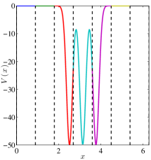
(a)

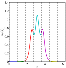
(b)

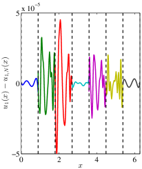
(c)

Figure 1. (a) The potential $V(x)$ given by the sum of three Gaussians with negative magnitude. (b) The first eigenfunction $u_{1}(x)$. (c) Point-wise error between the first eigenfunction $u_{1}(x)$ and the numerical solution $u_{1,N}(x)$ calculated using the ALB set with $7$ elements and $N=6$ basis functions per element.

Fig. 2 (a), (b) compare the error of the first $11$ eigenvalues and the corresponding eigenfunctions, together with the upper and lower estimators, respectively, using a relatively small number of $6$ basis functions per element. For the eigenfunctions, $C_{i,\eta}$ ranges from $1.50$ to $2.82$. Hence $\eta_{i}$ is indeed an effective upper bound for $|\!|\!|u_{i}-u_{i,N}|\!|\!|$. The lower bound estimator $C_{i,\xi}$ ranges from $0.32$ to $0.58$, and therefore is effective as well. In terms of eigenvalues, the upper bound estimator $C^{\lambda}_{i,\eta}$ ranges from $3.16$ and $9.70$, and the lower bound estimator for eigenvalues $C^{\lambda}_{i,\xi}$ ranges from $0.17$ to $0.40$. While the upper and lower bound of the eigenvalues remains to be true upper and lower bound, respectively, we note that the eigenvalue estimator is less effective compared to that of the eigenfunctions, and the upper (lower) bound estimator can overestimate (underestimate) the error by around one order of magnitude. Nonetheless, we note in Fig. 2 (a) that the error of eigenvalues spans over $4$ orders of magnitude, and our upper and lower estimators well captures such inhomogeneity in terms of accuracy among the different eigenvalues. The same trend is observed for eigenfunctions in Fig. 2 (b). Fig. 2 (b) also reports the terms ${\tt hot}^{\tt ub},{\tt hot}^{\tt lb}$ defined in Section 3. We find that ${\tt hot}^{\tt ub}_{i}$ and ${\tt hot}^{\tt lb}_{i}$ are significantly smaller than $\eta_{i}$ and $\xi_{i}$, respectively, and thus justify numerically that such terms are indeed high order terms.

Fig. 2 (c), (d) demonstrate the error of eigenvalues and eigenfunctions and the associated estimators using a more refined basis set, with $10$ basis functions per element. Despite the small increase of the number of basis functions, the error of eigenvalues is reduced to as low as $10^{-8}$. $C_{i,\eta}$ for eigenfunctions is between $2.19$ and $2.45$, and $C_{i,\xi}$ is between $0.64$ and $0.67$. The effectiveness parameters are remarkably homogeneous for all eigenfunctions computed. Correspondingly $C^{\lambda}_{i,\eta}$ for eigenvalues is between $5.27$ and $7.37$, and $C^{\lambda}_{i,\xi}$ for eigenvalues is between $0.45$ and $0.58$. The difference between $\eta_{i},\xi_{i}$ compared to ${\tt hot}^{\tt ub}_{i},{\tt hot}^{\tt lb}_{i}$ is amplified even further in Fig. 2 (d) as the basis set refines, and therefore justifies that ${\tt hot}^{\tt ub}_{i},{\tt hot}^{\tt lb}_{i}$ are indeed of higher order.

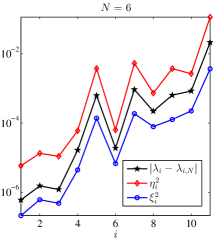
(a) $6$ basis

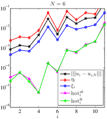
(b) $6$ basis

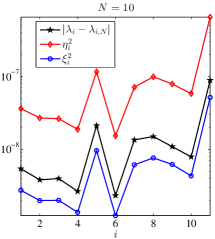
(c) $10$ basis

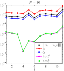
(d) $10$ basis

Figure 2. Error of the (a) eigenvalues and (b) eigenfunctions together with upper and lower bound estimator for the first $11$ eigenfunctions, using $6$ basis functions per element. (c),(d) are the same as (a),(b) respectively but with $10$ basis functions per element.

4.2. 2D example

Our second example is a 2D problem on $\Omega=[0,2\pi]\times[0,2\pi]$ with periodic boundary condition. The potential $V$ is given by the sum of four Gaussians with negative magnitude, as illustrated in Fig. 3 (a). Fig. 3 (b) shows the first eigenfunction $u_{1}$ and Fig. 3 (c) shows the point-wise error $u_{1}-u_{1,N}$ using $N=11$ ALBs per element. In the ALB computation, the domain is partitioned into $5\times 5$ elements, indicated by black dashed lines.

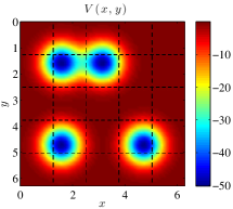
(a)

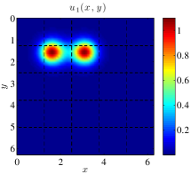
(b)

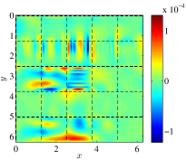
(c)

Figure 3. (a) The potential $V(x,y)$. (b) The first eigenfunction $u_{1}(x)$. (c) Point-wise error between the first eigenfunction $u_{1}(x)$ and the numerical solution $u_{1,N}(x)$ calculated using the ALB set with $5\times 5$ elements and $N=11$ basis functions per element.

Similar to the 1D case, Fig. 4 (a), (b) compare the error of the first $11$ eigenvalues and the corresponding eigenfunctions, together with the upper and lower estimators, respectively, using $11$ basis functions per element. The effectiveness parameter for eigenfunctions $C_{i,\eta}$ ranges from $2.78$ to $4.59$, and the $C_{i,\xi}$ ranges from $0.22$ to $0.36$. For the eigenvalues, the upper bound estimator $C^{\lambda}_{i,\eta}$ is between $12.73$ and $21.68$, and the lower bound estimator for eigenvalues $C^{\lambda}_{i,\xi}$ is between $0.08$ to $0.14$. Similarly, we observe that $C^{\lambda}_{i,\eta}$ and $C^{\lambda}_{i,\xi}$ are roughly on the order of magnitude of the square of the $C_{i,\eta}$ and $C_{i,\xi}$, respectively. Again our upper and lower bound estimator well captures the large inhomogeneity in terms of accuracy among different eigenvalues and eigenfunctions.

Fig. 4 (c), (d) show the error of eigenvalues and eigenfunctions and the associated estimators using a large number of $41$ basis functions per element. $C_{i,\eta}$ for eigenfunctions is between $2.00$ and $2.41$, and $C_{i,\xi}$ is between $0.23$ and $0.32$. The effectiveness parameters are remarkably homogeneous for all eigenfunctions computed. Correspondingly $C^{\lambda}_{i,\eta}$ for eigenvalues is between $4.45$ and $6.85$, and $C^{\lambda}_{i,\xi}$ for eigenvalues is between $0.06$ and $0.11$. The high order terms ${\tt hot}^{\tt ub}_{i},{\tt hot}^{\tt lb}_{i}$ are reported in Fig. 4 (b) and (d). Again we find that such terms are smaller than the upper and lower estimators, and the difference become more enhanced as the basis set refines.

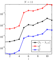
(a) $11$ basis

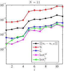
(b) $11$ basis

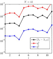
(c) $41$ basis

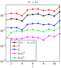
(d) $41$ basis

Figure 4. Error of the (a) eigenvalues and (b) eigenfunctions together with upper and lower bound estimator for the first $11$ eigenfunctions, using $11$ basis functions per element. (c),(d) are the same as (a),(b) respectively but with $41$ basis functions per element.

5. Conclusion

In this paper, we extend the framework that was introduced in the companion paper (Part I) [33] to linear eigenvalue problems for second order partial differential operators in a discontinuous Galerkin (DG) framework. Our method provides residual type a posteriori upper and lower bounds estimators for estimating the error of the numerically computed eigenvalues and eigenfunctions. The key-feature of our approach is that in absence of a priori inverse type inequalities for non-polynomial basis functions, local eigenvalue problems are solved and subsequently embedded in the a posteriori estimates. Hence our estimate is tailored for each new set of basis functions, and numerical results illustrate the effectiveness of our approach.

Future developments will naturally concern the extension to non-linear eigenvalue problems and in particular the Kohn-Sham equations in the framework density functional theory.

References

- [1] M. G. Armentano and R. G. Durán. Asymptotic lower bounds for eigenvalues by nonconforming finite element methods. Electron. Trans. Numer. Anal., 17:93–101, 2004.
- [2] I. Babuška and J. Osborn. Eigenvalue problems. In Handbook of numerical analysis, Vol. II, Handb. Numer. Anal., II, pages 641–787. North-Holland, Amsterdam, 1991.
- [3] N. W. Bazley and D. W. Fox. Lower bounds for eigenvalues of Schrödinger’s equation. Phys. Rev. (2), 124:483–492, 1961.
- [4] D. Boffi. Finite element approximation of eigenvalue problems. Acta Numer., 19:1–120, 2010.
- [5] E. Cancès, R. Chakir, and Y. Maday. Numerical analysis of the planewave discretization of some orbital-free and kohn-sham models. ESAIM: Mathematical Modelling and Numerical Analysis, 46:341–388, 3 2012.
- [6] E. Cancès, G. Dusson, Y. Maday, B. Stamm, and M. Vohralík. A perturbation-method-based a posteriori estimator for the planewave discretization of nonlinear Schrödinger equations. Comptes Rendus Mathematique, 352(11):941 – 946, 2014.
- [7] E. Cancès, G. Dusson, Y. Maday, B. Stamm, and M. Vohralík. Guaranteed and robust a posteriori bounds for Laplace eigenvalues and eigenvectors: conforming approximations. working paper or preprint, Sept. 2015.
- [8] C. Carstensen and J. Gedicke. Guaranteed lower bounds for eigenvalues. Math. Comp., 83(290):2605–2629, 2014.
- [9] R. G. Durán, C. Padra, and R. Rodríguez. A posteriori error estimates for the finite element approximation of eigenvalue problems. Math. Models Methods Appl. Sci., 13(8):1219–1229, 2003.
- [10] G. Dusson and Y. Maday. A Posteriori Analysis of a Non-Linear Gross-Pitaevskii type Eigenvalue Problem. 28 pages, Aug. 2013.
- [11] W. E and B. Engquist. The heterognous multiscale methods. Comm. Math. Sci., 1:87–132, 2003.
- [12] G. E. Forsythe. Asymptotic lower bounds for the fundamental frequency of convex membranes. Pacific J. Math., 5:691–702, 1955.
- [13] D. W. Fox and W. C. Rheinboldt. Computational methods for determining lower bounds for eigenvalues of operators in Hilbert space. SIAM Rev., 8:427–462, 1966.
- [14] M. J. Frisch, J. A. Pople, and J. S. Binkley. Self-consistent molecular orbital methods 25. supplementary functions for gaussian basis sets. J. Chem. Phys., 80:3265–3269, 1984.
- [15] S. Giani and E. J. C. Hall. An a posteriori error estimator for hp-adaptive discontinuous Galerkin methods for elliptic eigenvalue problems. Math. Mod. Meth. Appl. Sci., 22:1250030–1250064, 2012.
- [16] F. Goerisch and Z. Q. He. The determination of guaranteed bounds to eigenvalues with the use of variational methods. I. In Computer arithmetic and self-validating numerical methods (Basel, 1989), volume 7 of Notes Rep. Math. Sci. Engrg., pages 137–153. Academic Press, Boston, MA, 1990.
- [17] L. Grubišić and J. S. Ovall. On estimators for eigenvalue/eigenvector approximations. Math. Comp., 78(266):739–770, 2009.
- [18] V. Heuveline and R. Rannacher. A posteriori error control for finite approximations of elliptic eigenvalue problems. Adv. Comput. Math., 15(1-4):107–138, 2001.
- [19] R. Hiptmair, A. Moiola, and I. Perugia. Plane wave discontinuous Galerkin methods for the 2D Helmholtz equation: analysis of the p-version. SIAM J. Numer. Anal., 49:264–284, 2011.
- [20] T. Y. Hou and X.-H. Wu. A multiscale finite element method for elliptic problems in composite materials and porous media. J. Comput. Phys., 134:169–189, 1997.
- [21] J. Hu, Y. Huang, and Q. Lin. Lower bounds for eigenvalues of elliptic operators: by nonconforming finite element methods. J. Sci. Comput., 61(1):196–221, 2014.
- [22] J. Hu, Y. Huang, and Q. Shen. The lower/upper bound property of approximate eigenvalues by nonconforming finite element methods for elliptic operators. J. Sci. Comput., 58(3):574–591, 2014.
- [23] J. D. Joannopoulos, S. G. Johnson, J. N. Winn, and R. D. Meade. Photonic crystals: molding the flow of light. Princeton Univ. Pr., 2011.
- [24] J. Junquera, O. Paz, D. Sanchez-Portal, and E. Artacho. Numerical atomic orbitals for linear-scaling calculations. Phys. Rev. B, 64:235111–235119, 2001.
- [25] T. Kato. On the upper and lower bounds of eigenvalues. J. Phys. Soc. Japan, 4:334–339, 1949.
- [26] J. Kaye, L. Lin, and C. Yang. A posteriori error estimator for adaptive local basis functions to solve Kohn-Sham density functional theory. Commun. Math. Sci., 13:1741, 2015.
- [27] W. Kohn and L. Sham. Self-consistent equations including exchange and correlation effects. Phys. Rev., 140:A1133–A1138, 1965.
- [28] J. R. Kuttler and V. G. Sigillito. Bounding eigenvalues of elliptic operators. SIAM J. Math. Anal., 9(4):768–778, 1978.
- [29] J. R. Kuttler and V. G. Sigillito. Estimating eigenvalues with a posteriori/a priori inequalities, volume 135 of Research Notes in Mathematics. Pitman (Advanced Publishing Program), Boston, MA, 1985.
- [30] Y. A. Kuznetsov and S. I. Repin. Guaranteed lower bounds of the smallest eigenvalues of elliptic differential operators. J. Numer. Math., 21(2):135–156, 2013.
- [31] M. G. Larson. A posteriori and a priori error analysis for finite element approximations of self-adjoint elliptic eigenvalue problems. SIAM J. Numer. Anal., 38(2):608–625, 2000.
- [32] L. Lin, J. Lu, L. Ying, and W. E. Adaptive local basis set for Kohn-Sham density functional theory in a discontinuous Galerkin framework I: Total energy calculation. J. Comput. Phys., 231:2140–2154, 2012.
- [33] L. Lin and B. Stamm. A posteriori error estimates for discontinuous Galerkin methods using non-polynomial basis functions. Part I: Second order linear PDE. ESAIM: Mathematical Modelling and Numerical Analysis, 2015.
- [34] X. Liu and S. Oishi. Verified eigenvalue evaluation for the Laplacian over polygonal domains of arbitrary shape. SIAM J. Numer. Anal., 51(3):1634–1654, 2013.
- [35] Y. Maday and A. T. Patera. Numerical analysis of a posteriori finite element bounds for linear functional outputs. Math. Models Methods Appl. Sci., 10(5):785–799, 2000.
- [36] C. B. Moler and L. E. Payne. Bounds for eigenvalues and eigenvectors of symmetric operators. SIAM J. Numer. Anal., 5:64–70, 1968.
- [37] M. Plum. Guaranteed numerical bounds for eigenvalues. In Spectral theory and computational methods of Sturm-Liouville problems (Knoxville, TN, 1996), volume 191 of Lecture Notes in Pure and Appl. Math., pages 313–332. Dekker, New York, 1997.
- [38] R. Rannacher, A. Westenberger, and W. Wollner. Adaptive finite element solution of eigenvalue problems: balancing of discretization and iteration error. J. Numer. Math., 18(4):303–327, 2010.
- [39] I. Šebestová and T. Vejchodský. Two-sided bounds for eigenvalues of differential operators with applications to Friedrichs, Poincaré, trace, and similar constants. SIAM J. Numer. Anal., 52(1):308–329, 2014.
- [40] G. Still. Computable bounds for eigenvalues and eigenfunctions of elliptic differential operators. Numer. Math., 54(2):201–223, 1988.
- [41] R. Tezaur and C. Farhat. Three-dimensional discontinuous Galerkin elements with plane waves and Lagrange multipliers for the solution of mid-frequency Helmholtz problems. Int. J. Numer. Meth. Eng., 66:796–815, 2006.
- [42] R. Verfürth. A posteriori error estimates for nonlinear problems. Finite element discretizations of elliptic equations. Math. Comp., 62(206):445–475, 1994.
- [43] H. F. Weinberger. Upper and lower bounds for eigenvalues by finite difference methods. Comm. Pure Appl. Math., 9:613–623, 1956.
- [44] Y. Yang, J. Han, H. Bi, and Y. Yu. The lower/upper bound property of the Crouzeix–Raviart element eigenvalues on adaptive meshes. J. Sci. Comput., 62(1):284–299, 2015.