Linear and Nonlinear Frequency-Division Multiplexing

Abstract

Two signal multiplexing schemes for optical fiber communication are considered: Wavelength-division multiplexing (WDM) and nonlinear frequency-division multiplexing (NFDM), based on the nonlinear Fourier transform (NFT). Achievable information rates (AIRs) of NFDM and WDM are compared in a network scenario with an ideal lossless model of the optical fiber in the defocusing regime. It is shown that the NFDM AIR is greater than the WDM AIR subject to a bandwidth and average power constraint, in a representative system with one symbol per user. The improvement results from nonlinear signal multiplexing.

I Introduction

One factor limiting data rates in optical communication is that linear multiplexing is applied to the nonlinear optical fiber. To address this limitation, nonlinear frequency-division multiplexing (NFDM) was introduced [1, 2], [3, Sec. II]. NFDM is a signal multiplexing scheme based on the nonlinear Fourier transform (NFT), which represents a signal in terms of its discrete and continuous nonlinear Fourier spectra. In NFDM users’ signals are multiplexed in the nonlinear Fourier domain and propagate independently in a model of the optical fiber described by the lossless noiseless nonlinear Schrödinger (NLS) equation [1, 2, 3].

Prior work illustrates how NFDM is applied, with examples of achievable information rates (AIRs). However, an NFDM AIR higher than the corresponding one in a linear multiplexing has not yet been demonstrated. In this paper we consider an optical fiber network with an integrable model of the optical fiber in the defocusing regime. The main contribution of the paper is showing that the AIR of NFDM is greater than the AIR of wavelength-division multiplexing (WDM) for a given bandwidth and average signal power, in a representative system with one symbol per user.

AIRs of WDM and NFDM with continuous spectrum modulation were compared in [3, Sec. V. D, Fig. 9(b)]. In this work, although the signal of each user is modulated in the nonlinear Fourier domain, the signal of different users are multiplexed linearly. The reason was that the computational complexity of the inverse NFT, which is usually governed by integral equations, is high for data transmission. This made it difficult to perform both nonlinear modulation and multiplexing. As a consequence, NFDM expectedly achieved data rates approximately equal to WDM rates. It was explained that, to improve on WDM rates, one must consider a network scenario and multiplex users’ signals nonlinearly [4, Sec. 6.7. 1], [3, Secs. II.C, V. D. and VI. A].

To demonstrate NFDM high data rates, we first simplify the inverse NFT. Common approaches to the inverse NFT are based on integral equations, in sharp contrast to approaches to the forward NFT. The integral equations may also be cumbersome to solve, hindering the application of the NFT. In Section V, we interpret the inverse NFT as the dual of the forward NFT, as in the Fourier transform. With this perspective, the forward and inverse NFT can be computed using the forward and backward iteration of any integration scheme. This allows us to compute the inverse NFT naturally by running backward the algorithms for the forward NFT described in [2]. We compare the Boffetta-Osborne (BO) [5] and the Ablowitz-Ladik (AL) [6] integration schemes for the inverse NFT, and apply the AL scheme in Section VII.

Next we consider the NLS equation in the defocusing regime, which has several advantages. First, the operator $L$ in the Lax pair underlying the channel is self-adjoint. Consequently, solitons, the less tractable part of the NFT, are naturally absent. Second, numerical algorithms are robust in this regime. Third, the analyticity of the one of the nonlinear Fourier coefficients can be exploited to compute these coefficients from the NFT efficiently. Forth, it is easier to maximize the spectral efficiency (SE) when the discrete spectrum is absent, as explained below.

In the finite blocklength communication, a guard interval is typically introduced between consecutive data blocks in the time domain. When the discrete spectrum is absent, the NFT is a one-dimensional function similar to the Fourier transform. Consequently, the Nyquist-Shannon sampling theorem can be applied to systematically modulate all degrees-of-freedoms (DoFs) in a finite nonlinear bandwidth — namely, in the nonlinear Fourier domain, the signal consists of a train of raised-cosine functions as in [3, Eq. 2 & Sec. V. D]. In contrast, since it is yet unclear how to represent bandlimited $N$-solitons methodically, in practice $N$-soliton transmission is limited to small $N$. As a result, the ratio of the guard time to blocklength is smaller with the continuous spectrum modulation than that with the discrete spectrum modulation.

The paper is structured as follows. The literature on data transmission using the NFT is abundant. In Section II we review this literature, highlight the state-of-the-art, and put the present paper in context. In Section III we explain the origin of the limitation of the conventional methods in optical fiber networks. The forward and inverse NFT are presented in Section IV and Section V, respectively. The theoretical base of NFDM was presented in [1, 2, 3]. However, the theory simplifies considerably when the discrete spectrum is absent. In Section VI, we present an abstract approach to nonlinear modulation and multiplexing using the continuous spectrum. Here, in contrast to the linear modulation and multiplexing that are based on vector space representations, the signal space at the input of the channel is not represented by a vector space. AIRs of NFDM and WDM are numerically computed and compared in Section VII. Finally, the paper is concluded in Section VIII, followed by Appendices A and B which contain details.

Notation

Real, non-negative real, non-positive real, natural and complex numbers are denoted by $\mathbb{R}$, $\mathbb{R}_{0}^{+}$, $\mathbb{R}_{0}^{-}$, $\mathbb{N}$ and $\mathbb{C}$, respectively. The upper half complex plane is the open region $\mathbb{C}^{+}\stackrel{{\scriptstyle\Delta}}{{=}}\bigl{\{}\lambda\in\mathbb{C}:\Im(\lambda)>0\bigr{\}}$. Vectors are distinguished using the bold font, e.g., $\mathbf{x}\in\mathbb{R}^{n}$. The Lebesgue space of functions $f:\mathbb{R}\mapsto\mathbb{C}$ with finite $p-$norm $\left\lVert f\right\rVert_{L^{p}(\mathbb{R})}$ is represented by $L^{p}(\mathbb{R})$. The Hilbert space of $\mathcal{T}$-periodic complex-valued functions with the inner product $\langle f,g\rangle\stackrel{{\scriptstyle\Delta}}{{=}}\frac{1}{\mathcal{T}}\int_{0}^{\mathcal{T}}f(t)g^{*}(t)\mathrm{d}t$ is shown by $L^{2}_{p}([0,\mathcal{T}])$, where $*$ is complex conjugate. The probability distribution of a (zero-mean) complex circular-symmetric Gaussian random variable with variance $\sigma^{2}$ is denoted by $\mathcal{N}_{\mathbb{C}}\!\left(0,\sigma^{2}\right)$. The Fourier transform operator is $\mathcal{F}$, defined with the convention in [7, Eq. 1]. The Fourier transform and the NFT of a signal $q(t)$ are respectively denoted by $\mathcal{Q}(\omega)$, $\omega\stackrel{{\scriptstyle\Delta}}{{=}}2\pi f\in\mathbb{R}$, and $Q(\lambda)$, $\lambda\in\mathbb{C}$. By default, time, frequency and bandwidth are with respect to the Fourier transform; the corresponding terms in the NFT are “nonlinear time”, “nonlinear frequency” and “nonlinear bandwidth,” that will be defined formally in Section VI. Let $\mathcal{H}$ be a complex Hilbert space with an orthonormal basis $(\phi_{k})_{k\in\mathbb{N}}$. We say $N$ is zero-mean Gaussian noise on $\mathcal{H}$ if $N=\sum_{k}N_{k}\phi_{k}$, where $N_{k}\sim~{}\mathcal{N}_{\mathbb{C}}\!\left(0,\sigma^{2}_{k}\right)$ is a sequence of independent random variables. To simplify the notation, sometimes we add or drop variables in functions. For example, in Section V, $q(t)\stackrel{{\scriptstyle\Delta}}{{=}}q(t,z)$ and $a(\lambda)\stackrel{{\scriptstyle\Delta}}{{=}}a(\lambda,t)\stackrel{{\scriptstyle\Delta}}{{=}}a(\lambda,t,z)$.

II Transmission Using the NFT

II-A NFT in Optical Communication

The NFT has appeared in optical communication in assortment of places. The literature may be classified as approaches extending linear modulation to nonlinear modulation, and linear multiplexing to nonlinear multiplexing. This division clarifies concepts and explains the way that the NFT could usefully be applied to communications.

II-A1 Nonlinear modulation

Multi-soliton communication

One of the triumphs of the nonlinear science is soliton theory. The NFT is the central tool for the analysis of solitons. The fundamental soliton communication with on-off keying modulation played a pivotal role in the early years of optical communication. The fundamental soliton communication was extended to eigenvalue communication in [8], in order to transmit more than one bit in the time duration of a fundamental soliton. The observation was that the eigenvalues are conserved in the channel, while the amplitude and phase change. It is thus natural to modulate the invariant quantities, such as eigenvalues.

The 1-soliton communication can be systematically extended to modulating all DoFs in $N$-soliton communication [9, 3, 10, 11, 12]. This extension may be viewed as generalizing the conventional linear modulation in digital communication [13, Chap. 6] to nonlinear modulation in the optical fiber. However, although the AIR of $N$-soliton communication is naturally higher than the AIR of 1-soliton communication, it is equal to the AIR of any other good signal set with $N$ parameters. For instance, the widely-used pulse-amplitude modulation (PAM) with Nyquist pulse shape and an $N$-ary constellation achieves the same AIR. This is because the change of waveform in the channel is not a fundamental limitation in communications, since it is equalized at the receiver (as in the radio channels). Importantly, the same signal space may be generated by linear or nonlinear modulation.

In sum, nonlinear modulation (such as multi-soliton communication) does not have a fundamental advantage in terms of the AIR over linear modulation (such as the standard PAM) in any channel, under optimal receiver. On the contrary, linear modulation with equalization is preferred in nonlinear channels because it is simple.

Discrete and continuous spectrum modulation

The multi-soliton communication can be generalized to discrete and continuous spectrum modulation [3, 10, 14, 15]. However, DoFs in time, frequency, nonlinear time, and nonlinear frequency are in one-to-one correspondence. Thus, modulating both discrete and continuous spectra does not achieve a data rate higher than the present AIRs in coherent systems. In fact, both spectra are indirectly fully modulated in, e.g., Nyquist-WDM transmission. Existing approaches are not improved fundamentally by replacing the set of signal DoFs with another equivalent set.

II-A2 Nonlinear multiplexing

Finally, the NFT can be applied for signal multiplexing. For this purpose, NFDM was designed in [1, 2, 3] in order to address the limitation that the fiber nonlinearity sets on the AIRs of linear multiplexing in optical networks. In this approach, add-drop multiplexers (ADMs) in the network are replaced with nonlinear multiplexers constructed using the NFT. Importantly, data rates higher than WDM rates may be achieved using this approach.

As noted, modulating both spectra within each user but subsequently performing linear multiplexing of users’ signals will not achieve a data rate higher than the existing WDM rates. On the other hand, linearly modulating the signal of each user and performing nonlinear multiplexing of users’ signals can improve WDM rates. NFDM is an approach where modulation can be linear or nonlinear, but multiplexing is nonlinear.

Note that although the theoretical principle of the nonlinear multiplexing was presented in [1, 2, 3], the simulations in [3, Sec. V. D] are essentially nonlinear modulation, combined with linear multiplexing. It is the objective of the present paper to continue the simulations in [3] but with nonlinear multiplexing.

II-B Review

Data transmission using the NFT has been explored in numerous papers recently. We review some of these papers, highlighting the latest work.

The NFT consists of a discrete and a continuous spectrum. The discrete spectrum with few nonlinear frequencies is modulated in [16, 17, 3, 18, 19, 11, 20, 21, 22, 23], while the continuous spectrum is modulated in [3, 10, 14]. The feasibility of the joint discrete and continuous spectrum modulation is demonstrated in [24, 25, 26].

Noise models for nonlinear frequencies and spectral amplitudes are developed in [27, 28, 29, 30]. The probability distribution of the noise in the nonlinear Fourier domain is obtained in [31] for some special cases. The impact of noise and perturbations on NFT is studied in [32, 33, 16, 34, 35].

Computing the forward NFT is straightforward; several algorithms are proposed in [2, 5]. The inverse NFT finds applications in the fiber Bragg grating design, where in this literature several layer-peeling algorithms for the inverse NFT [36] are optimized [37, 38, 39, 40]. Fast NFTs are studied in [41, 42, 43, 44], where here computing the NFT is generally reviewed.

Transmission based on the NFT is extended from single polarization to dual polarization for the discrete spectrum in [45, 46] and for the continuous spectrum in [47]. The periodic NFT is explored in [48] for communications, using signals with one or two DoFs for which the inverse NFT can be computed analytically.

AIRs of the discrete and continuous spectrum modulation are reported, respectively, in [3, 49, 50, 11, 16] and [3, 51, 52, 53]. A lower bound on the SE of multi-solitons is obtained in [54]. However, these AIRs are obtained under strong assumptions; among others, the memory is neglected. Furthermore, often these AIRs are obtained for point-to-point channels and cannot be compared with the AIRs of the WDM networks. Correct analytic calculation of the maximum AIR in the nonlinear Fourier domain is still an open problem.

Transmission based on the NFT has been demonstrated in experiments, mostly with low data rates [18, 55, 56, 57, 12, 58, 59]. Aref, Bülow and Le conducted a series of experiments showing that one can modulate and demodulate nonlinear frequencies and spectral amplitudes [55, 56, 57]. Recent experiments from this group include joint discrete and continuous spectrum modulation [24] and an experiment modulating 222 nonlinear frequencies in the continuous spectrum reaching 2.3 bits/s/Hz and 125 Gbps  [60, 61].

Finally, while this paper was under review, the main result of the paper that NFDM can outperform WDM in simplified models in the defocusing regime has been confirmed in the focusing regime [62, 33], dual polarization transmission [47], and non-ideal models with perturbations [33]. These related works are based on the methodology established in this paper. However, a comprehensive comparison of WDM and NFDM in more general and realistic models is subject to research.

III Optical Fiber Networks

In this section, we present the channel model and explain the origin of the limitation of the conventional communication methods in this model.

III-A Network Model

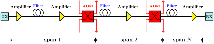
Figure 1: Block diagram of a network environment.

The propagation of a signal in the single-mode single-polarization optical fiber can be modeled by the stochastic NLS equation. The equation in the normalized form reads [1, Eqs. 1–3]

$$j\frac{\partial q}{\partial z}=\frac{\partial^{2}q}{\partial t^{2}}-2s|q|^{2}q+n(t,z),$$ (1)

where $q(t,z):\mathbb{R}\times\mathbb{R}_{0}^{+}\mapsto\mathbb{C}$ is the complex envelope of the signal as a function of time $t$ and distance $z$ along the fiber (the transmitter is located at $z=0$; the receiver is located at $z={\mathcal{L}}$), $n(t,z)$ is (zero-mean) white circular symmetric complex Gaussian noise, and $j\stackrel{{\scriptstyle\Delta}}{{=}}\sqrt{-1}$. Here, $s\stackrel{{\scriptstyle\Delta}}{{=}}-1$ in the focusing regime (corresponding to the standard fiber with anomalous dispersion) and $s\stackrel{{\scriptstyle\Delta}}{{=}}+1$ in the defocusing regime (corresponding to the fiber with normal dispersion).

The NLS equation (1) models the chromatic dispersion (captured by the term $\partial^{2}q/\partial t^{2}$), Kerr nonlinearity (captured by the term $|q|^{2}q$), and noise (that arises from distributed amplification along the fiber). We assumed that the fiber loss is perfectly compensated by Raman amplification so that (1) does not contain a loss term. The model (1) takes into account the the three leading physical effects in fiber; we refer the reader to [63] for some higher-order effects that are neglected in (1), and generally for modeling the optical fiber.

In this paper, we consider a network environment. This refers to a communication network with the following set of assumptions [3, Sec. II. B. 3]: (1) there are multiple transmitter (TX) and receiver (RX) pairs; (2) there are add-drop multiplexers (ADMs) in the network. The signal of the user-of-interest can co-propagate with the signals of the other users in part of the link. The location and the number of ADMs are unknown; (3) each TX and RX pair does not know the incoming and outgoing signals in the path that connects them. A network environment is depicted in Fig. 1.

To make use of the available fiber bandwidth, data can be modulated in disjoint frequency bands. As a result of using more bandwidth, data rates, measured in bits per second, were rapidly increased with the advent of WDM a few decades ago. However, the SE of WDM, measured in bits/s/Hz, is low, vanishing with the input power [64]. From the point of view of communication theory, WDM is a form of linear multiplexing, a fundamental concept forming the basis of the data transmission in most communication systems, including the fiber-optic systems.

There is a vast literature on WDM AIRs, sometimes referred to as the “nonlinear Shannon limit” [64]; see [65] and references therein. Fig. IV (b) shows the AIR of the WDM as a function of the average input power in a network environment. It can be seen that the AIR vanishes (or saturates in a modified scheme [66]) as the input power tends to infinity. The roll-off of the rate with power has been attributed to several factors [67], however there is consensus among researchers that the inter-channel interference arising from nonlinearity is the primary factor [65], [3, Sec. II].

III-B Origin of the Limitation of the Conventional Methods

It was realized in the past few years that nonlinear interactions do not limit the capacity in the deterministic models of optical networks. These interactions arise from methods of communication, which disregard nonlinearity [1, 2, 3]. After abstracting away non-essential aspects, current methods, in essence, apply linear modulation and multiplexing. The linear modulation schemes include PAM and pulse-train transmission. The linear multiplexing methods are WDM, orthogonal frequency-division multiplexing (OFDM), time-division multiplexing (TDM), polarization-division multiplexing (PDM) and space-division multiplexing (SDM). When linear multiplexing is applied to nonlinear channels, it gives rise to inter-channel interference and inter-symbol interference (ISI). In a network environment interference cannot be removed, while intra-channel ISI can partially be compensated using signal processing. The idea of sharing bandwidth in WDM, and integration in SDM, conflict with nonlinearity because of interactions among transmission modes. Since the nonlinearity is fixed by physics, it was proposed to replace the approach [1, 2, 3].

Yousefi and Kschischang recently proposed nonlinear frequency-division multiplexing which is fundamentally compatible with the channel [1, 2, 3]. NFDM exploits a delicate structure in the channel model, in order to implement interference-free communication. NFDM is based on the observation that the NLS equation supports nonlinear Fourier “modes” which have an important property that they propagate independently in the channel, the key to build a multi-user system. The tool necessary to reveal independent signal DoFs is the NFT. Based on the NFT, NFDM was constructed which can be viewed as a generalization of OFDM in linear channels to the nonlinear optical fiber. Exploiting the integrability property, NFDM modulates non-interacting signal DoFs in the channel.

IV Summary of NFDM

In this section, we review NFDM from [1, 2, 3].

Let $T:\mathcal{H}\mapsto\mathcal{H}$ be a compact (linear) map on a separable complex Hilbert space $\mathcal{H}$ with the inner product $<,>$. Consider the channel

$$Y\stackrel{{\scriptstyle\Delta}}{{=}}T(X)+N,$$ (2)

where $X$ is the input signal, $Y$ is the output signal and $N$ is Gaussian noise on $\mathcal{H}$. The channel can be discretized by projecting signals and noise onto an orthonormal basis $(\phi_{\lambda})_{\lambda\in\mathbb{N}}$ of $\mathcal{H}$

$$\bigl{\{}X,Y,N\bigr{\}}=\sum\limits_{\lambda=1}^{\infty}\bigl{\{}X_{\lambda},Y_{\lambda},N_{\lambda}\bigr{\}}\phi_{\lambda},$$ (3)

where $X_{\lambda},Y_{\lambda},N_{\lambda}\in\mathbb{C}$ are DoFs. This results in a discrete model

$$Y_{\lambda}=H_{\lambda}X_{\lambda}+\underbrace{\sum\limits_{\mu\neq\lambda}H_{\lambda\mu}X_{\mu}}_{\color[rgb]{0,0,0}\textnormal{linear interactions}}+N_{\lambda},$$ (4)

where $H_{\lambda\mu}=\langle T\phi_{\mu},\phi_{\lambda}\rangle$, $\lambda\in\mathbb{N}$. Depending on the choice of basis, interactions in (4) could refer to ISI in time, inter-channel interference in frequency, or generally interaction among DoFs in any of the methods in Fig. IV(a).

Suppose that $T$ is diagonalizable and has a set of eigenvectors forming an orthonormal basis of $\mathcal{H}$, e.g., when $T$ is self-adjoint [1, Thm. 6]. In this basis, interactions in (4) are zero and

$$Y_{\lambda}=H_{\lambda}N_{\lambda}+N_{\lambda},$$ (5)

where $H_{\lambda}\stackrel{{\scriptstyle\Delta}}{{=}}H_{\lambda\lambda}$ is an eigenvalue of $T$. As a result, the channel is decomposed into parallel independent scalar channels for $\lambda=1,2,\cdots$.

Interactions in (4) arise if the basis used for communication is not compatible with the channel. As a special case, let $\mathcal{H}=L^{2}_{p}([0,\mathcal{T}])$ and $T$ be the convolution map $T(X)\stackrel{{\scriptstyle\Delta}}{{=}}H(t)\convolution X(t)$, where $H(t)\in L^{1}(\mathbb{R})$ is the channel filter and $\convolution$ denotes convolution. The eigenvectors and eigenvalues of $T$ are

$$\phi_{\lambda}(t)=\frac{1}{\sqrt{\mathcal{T}}}\exp(-j\lambda\omega_{0}t),\quad\omega_{0}\stackrel{{\scriptstyle\Delta}}{{=}}\frac{2\pi}{\mathcal{T}},$$

and $H_{\lambda}\stackrel{{\scriptstyle\Delta}}{{=}}\mathcal{F}(H)(\lambda\omega_{0})$. The Fourier transform maps convolution to a multiplication operator according to (5), where $X_{\lambda}$, $Y_{\lambda}$ and $N_{\lambda}$ are Fourier series coefficients. Interference and ISI are absent in the Fourier basis. OFDM is a technology in which information is modulated in independent spectral amplitudes $X_{\lambda}$, $\lambda\in\mathbb{N}$.

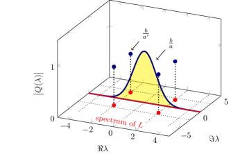
&      (a)         (b)

Figure 2: (a) Linear multiplexing methods. (b) Capacity bounds. The lower bound is the WDM AIR [3, Fig. 3]. (c) The absolute value of the NFT as a surface on the complex plane.

We explain NFDM in analogy with OFDM. First, we define the NFT as follows. Consider the operator

$$L\stackrel{{\scriptstyle\Delta}}{{=}}j\begin{pmatrix}\dfrac{\partial}{\partial t}&-q(t)\\ sq^{*}(t)&-\dfrac{\partial}{\partial t}\end{pmatrix},$$ (6)

where $q(t)\in L^{1}(\mathbb{R})$ is the signal. Let $\mathbf{v}(\lambda,t)\stackrel{{\scriptstyle\Delta}}{{=}}[v_{1},v_{2}]^{T}$ be an eigenvector of $L$ corresponding to the eigenvalue $\lambda$, i.e.,

$$L\mathbf{v}=\lambda\mathbf{v}.$$ (7)

The eigenvalues $\lambda$ of $L$ are called nonlinear frequencies. They are complex numbers whose real and imaginary parts have physical significance [3, Ex. 1]. Define the normalized eigenvector

$$\mathbf{u}(t,\lambda)\stackrel{{\scriptstyle\Delta}}{{=}}\begin{pmatrix}a(t,\lambda)\\ b(t,\lambda)\end{pmatrix},$$

where

$$a\stackrel{{\scriptstyle\Delta}}{{=}}e^{j\lambda t}v_{1},\quad b\stackrel{{\scriptstyle\Delta}}{{=}}e^{-j\lambda t}v_{2},$$ (8)

with the initial condition $\mathbf{u}(-\infty,\lambda)=\begin{pmatrix}1,0\end{pmatrix}^{T}$. The nonlinear Fourier coefficients are $a(\lambda)\stackrel{{\scriptstyle\Delta}}{{=}}a(\infty,\lambda)$ and $b(\lambda)\stackrel{{\scriptstyle\Delta}}{{=}}b(\infty,\lambda)$. The value of the NFT at the nonlinear frequency $\lambda\in\mathbb{R}$, called the spectral amplitude, is $b(\lambda)/a(\lambda)$.

If $\lambda$ is a simple eigenvalue in the upper half complex plane $\mathbb{C}^{+}$, it can be shown that $a(\lambda)=0$, so that the first term in the Taylor expansion of $a(\zeta)$ around $\zeta=\lambda$ vanishes [1, Sec. IV. B]. As a result, the spectral amplitude for $\lambda\in\mathbb{C}^{+}$ is $b/a^{\prime}$, where prime denotes differentiation, because $b/a$ is integrated out to its residue $b/a^{\prime}$ [1, App. F]. It can be shown that $a(\lambda)$ is an analytic function of $\lambda$ in $\mathbb{C}^{+}$ [1, Lem. 4]. Thus, nonlinear frequencies in $\mathbb{C}^{+}$ consist of the discrete set of (simple) zeros of $a(\lambda)$ denoted by $(\lambda_{i})_{i\in\mathcal{N}}$, where $\mathcal{N}\stackrel{{\scriptstyle\Delta}}{{=}}\{1,\cdots,N\}$, $N\in\mathbb{N}$. If $s=1$, the operator $L$ is self-adjoint; thus $\mathcal{N}$ is empty and nonlinear frequencies are real.

Definition 1 (Nonlinear Fourier Transform).

The NFT of $q(t)\in L^{1}(\mathbb{R})$ with respect to the $L$ operator (6) is a function $Q(\lambda)$ of the complex frequency $\lambda\in\mathbb{C}$, defined as

$$Q(\lambda)\stackrel{{\scriptstyle\Delta}}{{=}}\begin{cases}\dfrac{b(\lambda)}{a(\lambda)},&\lambda\in\mathbb{R},\\[10.00002pt] \dfrac{b(\lambda_{i})}{a^{\prime}(\lambda_{i})},&\lambda_{i}\in\mathbb{C}^{+},\quad i\in\mathcal{N}.\\ \end{cases}$$

The functions $\hat{q}(\lambda)\stackrel{{\scriptstyle\Delta}}{{=}}Q(\lambda)$, $\lambda\in\mathbb{R}$, and $\tilde{q}(\lambda_{i})\stackrel{{\scriptstyle\Delta}}{{=}}Q(\lambda_{i})$, $\lambda_{i}\in\mathbb{C}^{+}$, are called, respectively, the continuous and discrete spectrum.

∎

Let $Q(\lambda,z)$ be the NFT of $q(t,z)$ with respect to $t$. The important property of the NFT is that, if $q(t,z)$ propagates in (1) with noise set to zero, we have

$$Q(\lambda,{\mathcal{L}})=H(\lambda,{\mathcal{L}})Q(\lambda,0),$$ (9)

where $H(\lambda,\mathcal{L})\stackrel{{\scriptstyle\Delta}}{{=}}\exp(j4s\lambda^{2}{\mathcal{L}})$ is the all-pass-like channel filter. It follows that, just as the Fourier transform converts a linear convolutional channel into a number of parallel independent channels in frequency, the NFT converts the nonlinear dispersive channel (1) in the absence of noise into a number of parallel independent channels in nonlinear frequency. In NFDM information is modulated in independent spectral amplitudes $\operatorname{Q}(\lambda)$ for every $\lambda$. In the absence of noise, interference and ISI are simultaneously zero for all users of a multiuser network. Therefore, in contrast to WDM, the NFDM AIR is infinite in the deterministic model at any non-zero power.

V Computing the Inverse NFT

The standard approaches to the inverse NFT are based on the Riemann-Hilbert or Gelfand-Levitan-Marchenko integral equations [6, Ch. 2.2]. Naive numerical solution of these integral equations may be time-consuming or prone to error; optimized implementation requires attention to details of the numerical solution of the integral equations, which may produce a digression from the main purpose of using the NFT here. Consequently, we seek simpler, more natural and interpretable methods.

We interpret the inverse NFT as the dual of the forward NFT, as in the Fourier transform. We show that the forward and inverse NFT can be computed by running the iterations of any integration scheme, forward and backward in time. This allows us to use algorithms for the forward NFT for computing the inverse NFT, for example the Boffetta-Osborne and Ablowitz-Ladik schemes [2].

We emphasize that the two algorithms that are presented in this section are not new. They exists in applied mathematics [36], [5], are used in the literature of the fiber Bragg gratings design [37, 38], and revisited recently for fast implementation [42, 44]. However, their derivation in the literature has been made unnecessarily over-elaborate, as well as intertwined with the details of the physical application. The contribution of this section is to re-derive these existing algorithms using essentially a few lines of elementary analysis, in a simple and clear manner — compare the equation (38) with e.g., paper [37] or [36], [5]. Section V-A and V-B prior to (38) adapt the forward transform from [2].

The inverse NFT may be divided into three steps. First, from the NFT $Q(\lambda)$ we obtain $a(\lambda)$ and $b(\lambda)$. Second, from $a(\lambda)$ and $b(\lambda)$ we obtain $a(\lambda,t)$ and $b(\lambda,t)$. Third, we get $q(t)$ from $a(\lambda,t)$ and $b(\lambda,t)$.

Remark 1.

The NFT in [1] was presented for the focusing regime. The equations in [1] can often be extended from the focusing regime to the general case by substitutions

$$\{a,a^{*}\} \rightarrow \{a,a^{*}\},\qquad\{q,q^{*}\}$$ → {q, -sq^*},

$$\{b,b^{*}\} \rightarrow \{b,-sb^{*}\},\qquad\{\hat{q},\hat{q}^{*}\}$$ → {^q,-s^q^*}.

For example, the Parseval’s identity for the NFT is [1, Sec. IV. D. 8]

$$\int\limits_{-\infty}^{\infty}|q(t)|^{2}\mathrm{d}t=-\frac{s}{\pi}\int\limits_{-\infty}^{\infty}\log\left(1-s|\hat{q}(\lambda)|^{2}\right)\mathrm{d}\lambda.$$ (10)

This implies that $|\hat{q}(\lambda)|<1$ in the defocusing regime.

In this section, we drop the variable $z$ denoting the distance. Thus, $q(t)\stackrel{{\scriptstyle\Delta}}{{=}}q(t,z)$, $a(\lambda)\stackrel{{\scriptstyle\Delta}}{{=}}a(\lambda,z)$, etc.

∎

V-A Inverse Boffetta-Osborne Scheme

We shall begin with the Boffetta-Osborne integration scheme for the Zakharov-Shabat system, which is known to perform well for the forward NFT [5, 2]. This scheme is also called the continuous-time layer-peeling (CLP).

In the BO scheme, $q(t)$ is approximated by a piece-wise constant function. The NFT of a constant, and by induction a piece-wise constant, function can be computed analytically [1, Sec. IV. C]. Let $q(t)$ be a piece-wise constant function supported on $[T_{1},T_{2}]$. Discretize the time on the mesh

$$t[k]\stackrel{{\scriptstyle\Delta}}{{=}}T_{1}+k\epsilon,\quad k=0,\cdots,N-1,$$ (11)

where $\epsilon\stackrel{{\scriptstyle\Delta}}{{=}}T/N$, $T\stackrel{{\scriptstyle\Delta}}{{=}}T_{2}-T_{1}$, and set $q[k]\stackrel{{\scriptstyle\Delta}}{{=}}q(t[k])$. Recall that the forward iteration in the BO scheme is [2, Sec. III. C].

$$\mathbf{u}[k+1,\lambda]=\mathsf{M}[k,\lambda,q]\mathbf{u}[k,\lambda],\quad\mathbf{u}[0,\lambda]=\begin{pmatrix}1\\ 0\end{pmatrix},$$ (12)

where the monodromy matrix $\mathsf{M}$ is

$$\mathsf{M}[k,\lambda,q]\stackrel{{\scriptstyle\Delta}}{{=}}\begin{pmatrix}x[k]&\bar{y}[k]\\ y[k]&\bar{x}[k]\end{pmatrix},$$

in which [2, Eq. 11]:

$$x[k] \stackrel{{\scriptstyle\Delta}}{{=}} \Bigl{(}\cos(D\epsilon)-j\frac{\lambda}{D}\sin(D\epsilon)\Bigr{)}e^{j\lambda\left(t[k]-t[k-1]\right)},$$ (13)

$$y[k] \stackrel{{\scriptstyle\Delta}}{{=}} \frac{sq^{*}[k]}{D}\sin(D\epsilon)e^{-j\lambda(t[k]+t[k-1])},$$ (14)

where $D\stackrel{{\scriptstyle\Delta}}{{=}}\sqrt{\lambda^{2}-s|q[k]|^{2}}$ and

$$\bar{x}[k]\stackrel{{\scriptstyle\Delta}}{{=}}x^{*}[k](\lambda^{*}),\quad\bar{y}[k]\stackrel{{\scriptstyle\Delta}}{{=}}sy^{*}(\lambda^{*}).$$

It can be verified that $\det\mathsf{M}=1$.

The three steps of the inverse NFT via the BO scheme are as follows.

Step 1 (Factorization)

The first step is obtaining two parameters $a(\lambda)$ and $b(\lambda)$ from one parameter $Q(\lambda)$. Fundamentally, this is a Riemann-Hilbert factorization problem in the complex analysis [6, Ch. ]. Given $Q(\lambda)$, the Riemann-Hilbert integral equations in [1, Eq. 30] can be solved at $t=T$ to obtain $\mathbf{V}^{2}(T,\lambda)\stackrel{{\scriptstyle\Delta}}{{=}}\mathbf{u}=[a(\lambda),b(\lambda)]$. This requires solving a system of linear equations. This step does not incur a high computational cost, because the equations are solved only at one point $t=T$. Furthermore, in the defocusing regime, this step can be done more efficiently as follows.

From the unimodularity condition

$$\left|a(\lambda)\right|^{2}-s\left|b(\lambda)\right|^{2}=1,\quad\lambda\in\mathbb{R},$$ (15)

we obtain

$$\left|a(\lambda)\right|=\frac{1}{\sqrt{1-s|\hat{q}(\lambda)|^{2}}}.$$ (16)

Since $q(t)\in L^{1}(\mathbb{R})$, $a(\lambda)$ can be analytically extended to $\mathbb{C}^{+}$ [6, Lemma 2.1]. The real and imaginary parts of an analytic function are Hilbert transforms of one another. In Appendix B it is shown that in the defocusing regime $\log a(\lambda)$ can also be analytically extended to a region near the real line, thus amplitude $|a(\lambda)|$ and phase ${\rm{Arg}}(a(\lambda))$ are related by the Hilbert transform, i.e.,

$${\rm{Arg}}(a(\lambda))=\mathcal{H}\left(\log\left|a(\lambda)\right|\right),\quad\lambda\in\mathbb{R},$$ (17)

where $\mathcal{H}$ denotes the Hilbert transform and ${\rm{Arg}}$ is the principal value of the phase. As a result, we easily obtain $a$ and $b=\hat{q}a$ in the defocusing regime.

Step 2 (Integration)

The second step is to obtain $a(t,\lambda)$ and $b(t,\lambda)$ from $a(\lambda)$ and $b(\lambda)$. This step can be performed by integrating the Zakharov-Shabat system in negative time, i.e., by running the iterations for the forward NFT backward in time.

From (12), the backward iteration is:

$$\mathbf{u}[k,\lambda]=\mathsf{M}^{-1}[k,\lambda,q]\mathbf{u}[k+1,\lambda],\quad\mathbf{u}[N,\lambda]=\begin{pmatrix}a(\lambda)\\ b(\lambda)\end{pmatrix},$$ (18)

where $k=N-1,N-2,\cdots,0$, and

$$\mathsf{M}^{-1}[k,\lambda,q]=\begin{pmatrix}\bar{x}[k]&-\bar{y}[k]\\ -y[k]&x[k]\end{pmatrix}.$$

Computing $x[k]$ and $y[k]$ in (13) and (14) may involve evaluating $\cosh(x)$ for some $x$, when $s=1$. Moderate values of $x$, e.g., $x>25$, result in large numbers and numerical error. The numerical error may be reduced if the ratio $\hat{q}=b/a$ is updated, so that large numbers are canceled between $a$ and $b$. The forward iteration for $\hat{q}[k,\lambda]$ is

$$\hat{q}[k,\lambda] = \alpha[k]\frac{\bar{\beta}[k]+\hat{q}[k-1,\lambda]}{1+\beta[k]\hat{q}[k-1,\lambda]},\quad\hat{q}[0,\lambda]=0,$$

where

$$\alpha[k] \stackrel{{\scriptstyle\Delta}}{{=}} e^{-2j\lambda(t[k]-t[k-1])}\frac{1+\frac{j\lambda}{D}\tan(D\epsilon)}{1-\frac{j\lambda}{D}\tan(D\epsilon)},$$

$$\beta[k] \stackrel{{\scriptstyle\Delta}}{{=}} e^{2j\lambda t[k-1]}\frac{q[k]}{D}\frac{\tan(D\epsilon)}{1-\frac{j\lambda}{D}\tan(D\epsilon)},$$

and $\bar{\beta}[k]\stackrel{{\scriptstyle\Delta}}{{=}}s\beta^{*}[k](\lambda^{*})$. The backward iteration is

$$\hat{q}[k-1,\lambda]=\frac{\hat{q}[k,\lambda]-\bar{\beta}[k]\alpha[k]}{\alpha[k]-\beta[k]\hat{q}[k,\lambda]},\quad\hat{q}[N,\lambda]=\hat{q}(\lambda).$$

Step 3 (Signal Recovery)

From (7), $q(t)$ can be read off as

$$q^{*}(t) = s\frac{\partial_{t}v_{2}-j\lambda v_{2}}{v_{1}}$$ (19)

$$= se^{j2\lambda t}\frac{\partial_{t}b(t,\lambda)}{a(t,\lambda)},$$

where we used (8) (alternatively, see [2, Eq. 24]). Equation (19) constitutes the recovery relation.

The derivative term $\partial_{t}b$ in (19) incurs numerical error. It is preferred to recover $q(t)$ via a relation that does not involve derivative. From [1, Eq. 32], we have

$$q^{*}(t) = \frac{s}{\pi}\int\limits_{-\infty}^{\infty}\hat{q}(\lambda)e^{j2\lambda t}V_{2}^{1}(t,\lambda)\mathrm{d}\lambda,$$ (20)

where $\mathbf{V}^{1}\stackrel{{\scriptstyle\Delta}}{{=}}[V_{1}^{1},V_{2}^{1}]^{T}$ is a normalized eigenvector with the boundary condition $\mathbf{V}^{1}(+\infty,\lambda)=(1,0)^{T}$ [1, Eqs. 27 & 17(a)].

Fix $t$ and define

$$p_{t}(\tau)\stackrel{{\scriptstyle\Delta}}{{=}}\begin{cases}q(\tau),&\tau<t,\\[1.0pt] \frac{1}{2}q(t),&\tau=t,\\[1.0pt] 0,&\tau>t.\end{cases}$$ (21)

Applying (20) to $p_{t}(\tau)$ at $\tau=t$, we obtain

$$p^{*}_{t}(t) = \frac{s}{\pi}\int\limits_{-\infty}^{\infty}\hat{p}_{t}(\lambda)e^{j2\lambda t}\bar{V}_{2}^{1}(t,\lambda)\mathrm{d}\lambda$$ (22)

$$\overset{(a)}{=} \frac{s}{\pi}\int\limits_{-\infty}^{\infty}\hat{p}_{t}(\lambda)e^{j2\lambda t}\mathrm{d}\lambda$$

$$\overset{(b)}{=} \frac{s}{\pi}\int\limits_{-\infty}^{\infty}\hat{q}(t,\lambda)e^{j2\lambda t}\mathrm{d}\lambda,$$ (23)

where $\bar{\mathbf{V}}^{1}$ is an eigenvector of $p_{t}(\tau)$, $\hat{p}_{t}(\lambda)$ is the NFT of $p_{t}(\tau)$ and $\hat{q}(t,\lambda)\stackrel{{\scriptstyle\Delta}}{{=}}b(t,\lambda)/a(t,\lambda)$. Step $(a)$ follows because $p_{t}(\tau)=0$ for $\tau>t$, thus $\bar{V}^{1}_{2}(t,.)=\bar{V}^{1}_{2}(+\infty,.)=1$. Step $(b)$ follows because $\hat{q}(t,\lambda)$ is in one-to-one relation with $q(\tau)=p_{t}(\tau)$ for $\tau<t$, thus $\hat{p}_{t}(\lambda)=\hat{q}(t,\lambda)$. From (21) and (23)

$$q^{*}(t)=\frac{2s}{\pi}\int\limits_{-\infty}^{\infty}\hat{q}(t,\lambda)e^{j2\lambda t}\mathrm{d}\lambda.$$

Function $p_{t}(\tau)$ is in general discontinuous at $\tau=t$. From (22), $p^{*}_{t}(t)$ is described by a Fourier integral. At a point of discontinuity, the Fourier integral is the average of the value of the function on the two sides of that point. The choice $p(t)=q(t)/2$ in (21) ensures that (22) holds at the point of discontinuity.

It follows that

$$q^{*}[k]=\frac{2s}{\pi}\int\limits_{-\infty}^{\infty}\hat{q}[k,\lambda]e^{j2\lambda t[k]}\mathrm{d}\lambda,$$ (24)

where $\hat{q}[k,\lambda]\stackrel{{\scriptstyle\Delta}}{{=}}\hat{q}(t(k],\lambda)$. The integral in (24) can be discretized on the mesh

$$\lambda[m]\stackrel{{\scriptstyle\Delta}}{{=}}L_{1}+m\mu,\quad\quad m=0,\cdots,M-1,$$ (25)

where $\lambda\in[L_{1},L_{2}]$, $L\stackrel{{\scriptstyle\Delta}}{{=}}L_{2}-L_{1}$, and $\mu\stackrel{{\scriptstyle\Delta}}{{=}}L/M$.

Steps 3) and 2) are consecutively performed to obtain $q[k]$, for all $k$. Step 1) is performed initially if $\mathbf{u}[k,z]$ is updated instead of $\hat{q}[k,\lambda]$.

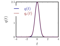
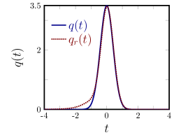
(a)            (b)            (c)

Figure 3: The Boffetta-Osborne scheme: (a) schematic diagram; (b,c) the result $q_{r}(t)$ of applying the forward-inverse NFT to Gaussian functions $q(t)$ with two amplitudes. The parameters are $T=L=64$ and $N=M=2048$.

In Section V-C we will show that the BO scheme, although suitable for the forward NFT, is inaccurate for the inverse NFT. As a result, below we consider the Ablowitz-Ladik scheme, where all variables are discrete and finite-dimensional. We may also refer to the AL scheme as the discrete layer-peeling (DLP).

V-B Inverse Ablowitz-Ladik Scheme

The AL discretization of the eigenproblem (7) is [2, Eq. 17]

$$\mathbf{v}[k+1,z] = c_{k}\begin{pmatrix}z^{\frac{1}{2}}&Q[k]\\ sQ^{*}[k]&z^{-\frac{1}{2}}\end{pmatrix}\mathbf{v}[k,z],$$ (26)

$$\mathbf{v}[0,z] = \begin{pmatrix}1\\ 0\end{pmatrix}z^{\frac{k_{0}}{2}},\quad 0\leq k\leq N-1,$$

where $z\stackrel{{\scriptstyle\Delta}}{{=}}\exp(-2j\lambda\epsilon)$, $Q[k]\stackrel{{\scriptstyle\Delta}}{{=}}\epsilon q[k]$, $c_{k}\stackrel{{\scriptstyle\Delta}}{{=}}1/\sqrt{1-s|Q[k]|^{2}}$, and $k_{0}\stackrel{{\scriptstyle\Delta}}{{=}}T_{1}/\epsilon$. Equation (8) suggests the following change of variable

$$a[k,z]\stackrel{{\scriptstyle\Delta}}{{=}}z^{-\frac{k_{0}+k}{2}}v_{1}[k,z],\quad b[k,z]\stackrel{{\scriptstyle\Delta}}{{=}}z^{\frac{k_{0}+k}{2}}v_{2}[k,z].$$ (27)

The variable $z$ in this section should not be confused with the distance.

Upon iterating (26)–(27), $a[k,z]$ and $b[k,z]$ are expressed as a linear combination of powers of $z^{\frac{1}{2}}$ and $z^{-\frac{1}{2}}$. We scale $a$ and $b$ to work with only the negative powers of $z$:

$$A[k,z]\stackrel{{\scriptstyle\Delta}}{{=}}a[k,z],\quad B[k,z]\stackrel{{\scriptstyle\Delta}}{{=}}z^{-(k_{0}+k)+\frac{1}{2}}b[k,z].$$ (28)

From (26), (27) and (28), we obtain the forward iteration for the scaled AL scheme

$$\begin{pmatrix}A[k+1,z]\\ B[k+1,z]\end{pmatrix} = c_{k}\begin{pmatrix}1&Q[k]z^{-1}\\ sQ^{*}[k]&z^{-1}\end{pmatrix}\begin{pmatrix}A[k,z]\\ B[k,z]\end{pmatrix},$$ (29)

$$\begin{pmatrix}A[0,z]\\ B[0,z]\end{pmatrix} = \begin{pmatrix}1\\ 0\end{pmatrix},\quad 0\leq k\leq N-1.$$

Note that $A[k,z]$ and $B[k,z]$ are polynomials of $z^{-1}$ with finite degrees.

Instead of updating $A[k,z]$ and $B[k,z]$ in (29) for each $z$, we can update the polynomial coefficients. The $z$-transforms of $A$ and $B$ are

$$A[k,z] = \sum\limits_{m=0}^{\bar{M}-1}A_{m}[k]z^{-m},$$ (30a)

$$B[k,z] = \sum\limits_{m=0}^{\bar{M}-1}B_{m}[k]z^{-m},$$ (31a)

where $\bar{M}\in\mathbb{N}$ is the number of non-zero coefficients, and $A_{m}[k]$ and $B_{m}[k]$ are calculated as

$$A_{m}[k] = \frac{1}{L}\int\limits_{L_{1}}^{L_{2}}A[k,e^{-2j\lambda t[k]}]e^{-j2m\epsilon\lambda}\mathrm{d}\lambda.$$ (32)

If $a[k,z]=A[k,z]$ is obtained via (29), then $\bar{M}<\infty$, and $a[k,z]$ approximates $a(t,z)$. If $a[k,z]$ is obtained by discretizing $a(t,\lambda)$ — namely, $a[k,.]$ equals to $a(k\epsilon,.)$ for some $k$— then in general $\bar{M}=\infty$.

The variable $z=z(\lambda)$ is the nonlinear frequency. The variable $m\in\bigl{\{}0,\cdots,\bar{M}-1\bigr{\}}$ may be viewed as the nonlinear time, the Fourier-conjugate of the nonlinear frequency $z$. Define the vector of the samples of $A[k,z(\lambda)]$ in the nonlinear frequency $\lambda$

$$\mathbf{\hat{A}}[k]\stackrel{{\scriptstyle\Delta}}{{=}}\begin{pmatrix}A[k,e^{-j2\lambda[0]t[k]}]&\cdots&A[k,e^{-j2\lambda[M-1]t[k]}]\end{pmatrix},$$ (33)

and the corresponding vector in the nonlinear time

$$\mathbf{A}[k] \stackrel{{\scriptstyle\Delta}}{{=}} \begin{pmatrix}A_{0}[k],\cdots,A_{\bar{M}-1}[k]\end{pmatrix}.$$

Let us discretize the integral in (32) in $\lambda$ on the mesh (25), choosing for the rest of the paper

$$M=\bar{M}=N,\quad L=\pi/\epsilon,\quad\mu=\pi/T.$$

We obtain that $\mathbf{A}[k]$ and $\mathbf{\hat{A}}[k]$ are the scaled nonlinear Fourier coefficients in the temporal and frequency domains, and

$$\mathbf{A}=\frac{1}{M}\mathbf{e}\circ\textnormal{DFT}(\mathbf{\hat{A}}),$$ (34)

where DFT is the discrete Fourier transform (with zero-based indexing), $\circ$ is the Hadamard product, and

$$\mathbf{e}\stackrel{{\scriptstyle\Delta}}{{=}}(1,e^{-j2\pi\frac{L_{1}}{L}},\cdots,e^{-j2\pi\frac{L_{1}}{L}(M-1)}).$$

Similar relations hold for the coefficient $B$.

The three steps of the inverse NFT via the AL scheme are as follows.

Step 1 (Factorization)

First we compute $a(N,\lambda)\stackrel{{\scriptstyle\Delta}}{{=}}a(\lambda)$ and $b(N,\lambda)\stackrel{{\scriptstyle\Delta}}{{=}}b(\lambda)$ from $Q(\lambda)$ according to the procedure outlined in Step 1 in the BO scheme. Then we calculate the frequency domain vectors $\mathbf{\hat{A}}[N]$ and $\mathbf{\hat{B}}[N]$ from (28) and (33), and the time domain vectors $\mathbf{A}[N]$ and $\mathbf{B}[N]$ from (34). The coefficients $A_{m}[N]$ and $B_{m}[N]$ are generally non-zero for all $m\geq 0$. Here, these sequences must be truncated.

Step 2 (Integration)

From (29), the backward iteration in the frequency domain $z$ is

$$\begin{pmatrix}A[k,z]\\ B[k,z]\end{pmatrix} = c_{k}\begin{pmatrix}1&-Q[k]\\ -sQ^{*}[k]z&z\end{pmatrix}\begin{pmatrix}A[k+1,z]\\ B[k+1,z]\end{pmatrix},$$ (35)

where $k=N-1,N-2,\cdots,0$. From (35), the backward iteration in the temporal domain is

$$\mathbf{A}[k] = c_{k}\Bigl{(}\mathbf{A}[k+1]-Q[k]\mathbf{B}[k+1]\Bigr{)},$$

$$\mathbf{B}[k] = c_{k}\operatorname{shift}\Bigl{(}-sQ^{*}[k]\mathbf{A}[k+1]+\mathbf{B}[k+1]\Bigr{)},$$

where $\operatorname{shift}(\mathbf{x})\stackrel{{\scriptstyle\Delta}}{{=}}(x_{2},\cdots,x_{n},0)$ is the left shift of $\mathbf{x}\stackrel{{\scriptstyle\Delta}}{{=}}(x_{1},x_{2},\cdots,x_{n})$.

The continuous-frequency unimodularity condition (15) on the unit circle $|z|=1$ is

$$\bigl{|}A[k,z]\bigr{|}^{2}-s\bigl{|}B[k,z]\bigr{|}^{2}=1.$$ (36)

In the temporal domain

$$\mathbf{A}\convolution\reflectbox{$\vec{\reflectbox{$\mathbf{A}$}}$}^{*}-s\mathbf{B}\convolution\reflectbox{$\vec{\reflectbox{$\mathbf{B}$}}$}^{*}=\boldsymbol{\delta},$$ (37)

where $\boldsymbol{\delta}\in\mathbb{R}^{2M-1}$ is the all-zero vector except for a one in the middle, $\convolution$ is vector convolution, and   $\vec{\reflectbox{$$}}$   is the flip operator, e.g., $\reflectbox{$\vec{\reflectbox{$\mathbf{A}$}}$}_{m}=\mathbf{A}_{M-m-1}$. The condition (36) or (37) can be checked in iterations to monitor the numerical error.

Step 3 (Signal Recovery)

The discretization of $\hat{q}(t,\lambda)=\exp(-2j\lambda t)(v_{2}/v_{1})$ on the time mesh (11) suggests to consider $\hat{q}[k,z]\stackrel{{\scriptstyle\Delta}}{{=}}z^{k_{0}+k}v_{2}[k,z]/v_{1}[k,z]$. We have

$$\hat{q}[k+1,z] = z^{k_{0}+k+1}\frac{v_{2}[k+1,z]}{v_{1}[k+1,z]}$$

$$= z^{k_{0}+k+1}\frac{sQ^{*}[k]v_{1}[k,z]+z^{-\frac{1}{2}}v_{2}[k,z]}{z^{\frac{1}{2}}v_{1}[k,z]+Q[k]v_{2}[k,z]}$$

$$= z^{k_{0}+k+\frac{1}{2}}\frac{sQ^{*}[k]+z^{-\frac{1}{2}}\left(\dfrac{v_{2}[k,z]}{v_{1}[k,z]}\right)}{1+z^{-\frac{1}{2}}Q[k]\left(\dfrac{v_{2}[k,z]}{v_{1}[k,z]}\right)}.$$

By induction, we can see that $\deg(v_{1})>\deg(v_{2})$ for $k\geq 1$, where $\deg(v)$ is the highest positive power of $z$ in $v$. Thus $\lim\limits_{z\rightarrow\infty}v_{2}[k,z]/v_{1}[k,z]=0$ and

$$Q^{*}[k] = s\lim\limits_{z\rightarrow\infty}z^{-k_{0}-k-\frac{1}{2}}\hat{q}[k+1,z]$$ (38)

$$= s\lim\limits_{z\rightarrow\infty}z^{-k_{0}-k-\frac{1}{2}}\frac{b[k+1,z]}{a[k+1,z]}$$

$$= s\frac{B[k+1,\infty]}{A[k+1,\infty]}$$

$$= s\frac{B_{0}[k+1]}{A_{0}[k+1]}.$$

Equating (38) basically follows from equating the like powers of $z$ in (29).

The AL scheme is summarized in Algorithm 1.

Algorithm 1 The AL scheme for the inverse NFT.

  Obtain $a(\lambda)$ and $b(\lambda)$ from $\hat{q}(\lambda)$, using (16) and (17). Set $a[N,\lambda]\stackrel{{\scriptstyle\Delta}}{{=}}a(\lambda)$ and $b[N,\lambda]\stackrel{{\scriptstyle\Delta}}{{=}}b(\lambda)$

  Compute $\mathbf{\hat{A}}[N]$ and $\mathbf{\hat{B}}[N]$ from (28) and (33), and $\mathbf{A}[N]$ and $\mathbf{B}[N]$ from (34). Truncate $\mathbf{A}[N]$ and $\mathbf{B}[N]$ to finite-dimensional vectors.

  for  $k=N,N-1,\cdots,1$ do

     Obtain $Q[k]$ from (38) or (42), and $q[k]=Q[k]/\epsilon$.

     Update

$$\mathbf{A} \leftarrow c_{k}\bigl{(}\mathbf{A}-Q[k]\mathbf{B}\bigr{)},$$

$$\mathbf{B} \leftarrow c_{k}\operatorname{shift}\bigl{(}-sQ^{*}[k]\mathbf{A}+\mathbf{B}\bigr{)}.$$

  end for

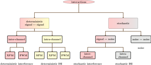
(a)      (b)

Figure 4: (a) Multi-user NFDM. (b) Interactions in linear multiplexing. Interactions that cannot be removed are identified with red. Interactions that can partly be equalized using signal processing are shown by yellow. Grey terms are addressed by coding. SPM and XPM stand for self- and cross-phase modulation, and FWM is four-wave mixing.

V-C Complexity, Accuracy and Remarks

V-C1 Complexity

Computing the Fourier integral or the NFT amounts to performing an integration; see (7). There are two variables $t$ and $\lambda$. If each variable is discretized in a mesh with $N$ points, there are $N^{2}$ points in a rectangular mesh in the $t-\lambda$ plane. Therefore, the basic algorithms for computing the Fourier transform or the NFT take $O(N^{2})$ operations — including the AL and BO schemes in this paper. This complexity, of course, is reduced to $O(N\log N)$ in the Fourier transform and, in some cases, to $O(N\log^{2}N)$ in the NFT [37, 44]. The least complexity NFT is subject to ongoing research.

V-C2 Accuracy

There are two sources of error in the BO scheme. First, the function $q(t)$ is approximated by a piece-wise constant function — once this approximation is made, the BO scheme is exact for the piece-wise constant function. The error in this part is $O(\epsilon)$ for smooth $q(t)$. Second, the integral (24) has to be discretized which is subject to error. Furthermore, here the discontinuity of $q(t)$ results in numerical errors when evaluating the Fourier integral (24) due to the Gibbs effect. Consequently, Step 3 is inexact. The error in this part depends on how the integral (24) is evaluated. Steps 1 and 2, on the other hand, are exact in the BO scheme.

Figs. 3 (b–c) show the result of applying the forward NFT followed by the inverse NFT to a Gaussian function using the BO scheme in the defocusing regime. It can be seen that the error is increased with the signal amplitude. Importantly, the local error accumulates as the iteration proceeds towards $t=T_{1}$. The BO scheme is sensitive to i) spectral parameters $L$ and $M$ and, to a smaller extent, temporal variables $T$ and $N$; and ii) the accuracy of the computing the integral (24).

In the AL scheme, Steps 2 and 3 are exact. Here too there are two sources of error. First, the continuous-time operator $L$ is approximated by its AL discretization. The error in this part is $O(\epsilon)$ for smooth functions. Second, the vectors $\mathbf{A}[N]$ and $\mathbf{B}[N]$ are truncated to finite-dimensional vectors in Step 1. The error in this part depends on the coefficients that are neglected. Note that Steps 2 and 3 are performed consecutively. Since these steps are exact, the error does not accumulate in the AL scheme. The step that is subject to error is Step 1 which is outside the iteration. Therefore, the error can be controlled in the AL scheme.

V-C3 Remarks

The AL discretization is obtained by approximation $1-2j\lambda$ in the first-order Euler discretization with $\exp(-j2\lambda\epsilon)$ [2, Sec. III. E]. This approximation makes eigenvectors a periodic function of $\lambda$ with period $L=\pi/\epsilon$. This is in contrast to the BO scheme where $L$ is arbitrary.

In the forward AL scheme, $\mathbf{A}[k]$ and $\mathbf{B}[k]$ have finite lengths and satisfy the discrete-frequency unimodularity condition (36). However, in the inverse NFT, while $a(\lambda)$ and $b(\lambda)$ are obtained from the continuous-frequency unimodularity condition (15), the truncated $\mathbf{A}[N]$ and $\mathbf{B}[N]$ do not generally satisfy the discrete-frequency unimodularity condition (37). In general, $\mathbf{A}[N]$ and $\mathbf{B}[N]$ should be realizable, i.e., they should be the image of $\mathbf{A}[0]$ and $\mathbf{B}[0]$ for some signal [37]. The AL scheme is improved if (36) is enforced in the backward iteration. It has been shown that this minor modification notably improves the algorithm, because it prevents the numerical error from propagating in the iteration [37].

In the AL scheme, $\mathbf{v}[N,z]$ depends on $\mathbf{v}[0,z]$ with the scale factor $\prod c_{k}=\exp(P)$, where

$$P\stackrel{{\scriptstyle\Delta}}{{=}}-\frac{1}{2}\sum\limits_{k=1}^{N}\log\left(1-s\left|Q[k]\right|^{2}\right).$$

As $N\rightarrow\infty$, $\epsilon$, $Q[k]$ and $P$ tend to zero. As a heuristic condition, we require that

$$0\leq P<P_{\max}$$ (39)

for a moderate $P_{\max}$, and

$$|Q[k]|<1.$$ (40)

It can be shown that

$$\frac{\mathrm{d}|Q[k-1]|}{\mathrm{d}|Q[k]|}\propto\frac{1}{\left(1-s|Q[k]|^{2}\right)^{2}}.$$

It is thus desirable to have

$$|Q[k]|\ll 1,$$ (41)

so that $Q[k-1]$ is not sensitive to error in $Q[k]$.

The AL scheme can be implemented in the frequency domain $z$ as well. Instead of updating $\mathbf{A}[k]$ and $\mathbf{B}[k]$, one could update $\mathbf{\hat{A}}[k]$ and $\mathbf{\hat{B}}[k]$. The accuracy of the AL scheme stems from the fact that it works with finite-dimensional vectors, and from the exactness of the Step 2 and 3, not from the implementation in the temporal domain.

The recovery relation (38) can be obtained in alternative ways. In Appendix A, both (38) and the following recovery relation are proved by induction

$$Q[k]=\frac{A_{k}[k+1]}{B_{k}[k+1]}.$$ (42)

Finally, (38) can also be obtained via discretizing (19), by replacing $\exp(j2\lambda t)$ with $z^{-k-k_{0}}$, $\partial_{t}$ with $z^{1/2}/\epsilon$, and equating the zeroth-order term in the $z$ expansion of both sides (corresponding to $z\rightarrow\infty$ or $\lambda\rightarrow\infty$ in $\mathbb{C}^{+}$). Both (38) and (42) follow basically by equating the like powers of $z$ in $v[k,z]$ in the AL scheme.

The BO scheme that is proposed in [5] is a first-order Euler integration scheme — except that, for the Zakharov-Shabat system in question, each step in integration can be done analytically without approximation. It generally applies well to differential equations which are exactly solvable in the special case that coefficients are constant.

The BO and AL schemes are simple first-order integration schemes. They can be extended to higher-order integration schemes in straightforward ways to compute the NFT arbitrary accurately (at the expense of performing more operations). We do not pursue more accurate or faster algorithms in this paper.

VI Linear and Nonlinear Frequency-Division Multiplexing

The theoretical underpinning of NFDM with discrete and continuous spectrum is presented in [1, 2, 3]. However, the theory simplifies considerably when the discrete spectrum is absent. In this section, we simplify NFDM with the continuous spectrum and present a general approach to nonlinear modulation and multiplexing (valid in the focusing and defocusing regimes).

VI-A Linear Modulation and Multiplexing

Let $\mathcal{H}$ be a complex Hilbert space with a basis $(\phi_{\ell})_{\ell}$, $\left\lVert\phi_{\ell}\right\rVert=1$. Linear modulation on $\mathcal{H}$ corresponds to $x\stackrel{{\scriptstyle\Delta}}{{=}}\sum_{\ell}s_{\ell}\phi_{\ell}$, where $s_{\ell}\in\mathbb{C}$ are symbols. If the basis is orthogonal, the demodulation is performed efficiently per-symbol as $s_{\ell}=\langle x,\phi_{\ell}\rangle$. The basis elements are sometimes called (linear-algebraic) transmission modes.

Let $\mathcal{H}_{k}$ be disjoint subspaces of $\mathcal{H}$ (excluding the zero element). Linear multiplexing of $x_{k}\in\mathcal{H}_{k}$ corresponds to $x\stackrel{{\scriptstyle\Delta}}{{=}}\sum_{k}x_{k}$. If $\mathcal{H}_{k}$ are pair-wise orthogonal, the demultiplexing is simply $x_{k}=P_{\mathcal{H}_{k}}(x)$, where $P_{\mathcal{H}_{k}}$ is the orthogonal projection onto $\mathcal{H}_{k}$. Clearly, $x_{k}$ need not be linearly modulated within $\mathcal{H}_{k}$.

Signals that are orthogonal at the channel input may not be orthogonal at the channel output. As a result, linear modulation and multiplexing are generally subject to ISI and interference — even in the linear channels. Suppose that the channel is governed by a compact (linear) self-adjoint map $T$ in the absence of noise. Then $(\phi_{\ell})_{\ell}$ can be chosen to be the set of orthogonal eigenvectors of $T$, for which the ISI is absent under per-symbol demodulation. Similarly, if $\mathcal{H}_{k}$ are chosen to be the span of disjoint subsets of orthogonal eigenvectors of $T$, interference is absent in demultiplexing by projection.

In linear modulation and multiplexing the set of signals that are transmitted in the channel (i.e., in the time domain) is represented by a vector space. We next consider NFDM where this signal space is not a linear space.

VI-B Nonlinear Modulation and Multiplexing Using the Continuous Spectrum

Nonlinear modulation and multiplexing using the NFT consists of linear modulation and multiplexing in the nonlinear Fourier domain. In what follows, we consider a multi-user system with $N_{u}$ users and $N_{s}$ symbols per user. Linear and nonlinear (passband) bandwidths are denoted, respectively, by $B$ and $W$.

VI-B1 Signal Spaces

Let $\hat{\mathcal{Q}}$ be the space of signals $\hat{q}(\lambda,z):\mathcal{W}\times\mathbb{R}_{0}^{+}\mapsto\mathbb{D}$, where $\mathcal{W}\stackrel{{\scriptstyle\Delta}}{{=}}[-\pi W,\pi W]$, and

$$\mathbb{D}\stackrel{{\scriptstyle\Delta}}{{=}}\begin{cases}\mathbb{C},&s=-1,\\ \mathbb{T},&s=+1,\end{cases}$$

where $\mathbb{T}$ is the open unit disk $\mathbb{T}\stackrel{{\scriptstyle\Delta}}{{=}}\bigl{\{}z\in\mathbb{C}\>:\>|z|<1\bigr{\}}$. Note that, from (10), if $s=1$, $|\hat{q}(\lambda,z)|<1$.

In the defocusing regime, $\hat{\mathcal{Q}}$ is not a vector space (with addition and multiplication), and not best suited for a communication theory. We introduce a transformation $F:\hat{q}(\lambda,z)\mapsto U(\lambda,z)$ so as to map $\mathbb{D}$ to $\mathbb{C}$. An appropriate choice motivated by (10) is

$$U(\lambda,z)\stackrel{{\scriptstyle\Delta}}{{=}}\left(-2s\log(1-s\left|\hat{q}(\lambda,z)\right|^{2})\right)^{\frac{1}{2}}e^{j{\rm{Arg}}(\hat{q}(\lambda,z))},$$ (43)

where ${\rm{Arg}}(\hat{q})$ is the phase of $\hat{q}$. We choose the image $\mathcal{U}$ of $F:\hat{\mathcal{Q}}\mapsto\mathcal{U}$ to be the vector space of finite-energy signals supported on $\mathcal{W}$. Transformation (43) is required in the defocusing regime. In the focusing regime, it is not required, however it makes the signal energy in time, frequency, nonlinear time and nonlinear frequency the same according to (49). This property is convenient for modulation.

VI-B2 NFDM Transmitter

Partition the space $\mathcal{U}=\bigcup_{k}\mathcal{U}_{k}$ into orthogonal user subspaces $(\mathcal{U}_{k})_{k=k_{1}}^{k_{2}}$, where user $k$ operates in the subspace $\mathcal{U}_{k}$ spanned by the orthogonal basis $(\Phi_{\ell}^{k}(\lambda))_{\ell=\ell_{1}}^{\ell_{2}}$, $\left\lVert\Phi_{\ell}^{k}(\lambda)\right\rVert^{2}=2\pi$. Here, $k$ is the user index, $\ell$ is the symbol index and

$$k_{1}\stackrel{{\scriptstyle\Delta}}{{=}}-\Bigl{\lfloor}\frac{N_{u}}{2}\Bigr{\rfloor},\quad k_{2}\stackrel{{\scriptstyle\Delta}}{{=}}\Bigl{\lceil}\frac{N_{u}}{2}\Bigr{\rceil}-1,$$

where $\lfloor x\rfloor$ and $\lceil x\rceil$ denote, respectively, rounding $x\in\mathbb{R}$ to nearest integers towards minus and plus infinity. Similar relations hold for $\ell_{1}$ and $\ell_{2}$ in terms of $N_{s}$.

The transmitted signal in the nonlinear frequency domain is

$$U(\lambda,0)\stackrel{{\scriptstyle\Delta}}{{=}}\underbrace{\sum\limits_{k=k_{1}}^{k_{2}}}_{\textnormal{linear mux}}\underbrace{\left(\sum\limits_{\ell=\ell_{1}}^{\ell_{2}}s_{\ell}^{k}\Phi_{\ell}^{k}(\lambda)\right)}_{\textnormal{linear mod.}},$$ (44)

where $(s_{\ell}^{k})_{\ell=\ell_{1}}^{\ell_{2}}$ are symbols of the user $k$. As discussed in Section II-A, the modulation in (44) can be linear or nonlinear, whereas the orthogonal multiplexing is required in NFDM.

In general, user signals can overlap in any domain. Interference in user $k$ is in the orthogonal subspace $\mathcal{U}_{k}^{\perp}$ and can be projected out. However, for the rest of the paper, we consider the special case where users operate in equally-spaced non-overlapping intervals of width $W_{0}\stackrel{{\scriptstyle\Delta}}{{=}}W/N_{u}$ Hz in the nonlinear frequency $l\stackrel{{\scriptstyle\Delta}}{{=}}\lambda/2\pi$. User $k$ is centered at the nonlinear frequency $l=kW_{0}$ and operates in the nonlinear frequency interval

$$\mathcal{W}_{k}\stackrel{{\scriptstyle\Delta}}{{=}}\bigl{[}kW_{0}-\frac{W_{0}}{2}\>,\>kW_{0}+\frac{W_{0}}{2}\bigr{]},\quad k_{1}\leq k\leq k_{2}.$$

In this case, $\Phi^{k}_{\ell}(\lambda)\stackrel{{\scriptstyle\Delta}}{{=}}\Phi_{\ell}(\lambda-2\pi kW_{0})$ where $(\Phi_{\ell}(\lambda))_{\ell=\ell_{1}}^{\ell_{2}}$ is an orthogonal basis for signals supported on $\mathcal{W}_{0}$.

Taking the inverse Fourier transform $\mathcal{F}^{-1}$ of (44) with respect to $\lambda$

$$u(\tau,0) \stackrel{{\scriptstyle\Delta}}{{=}} \mathcal{F}^{-1}(U(\lambda,0))$$ (45)

$$= \sum\limits_{k=k_{1}}^{k_{2}}\left(\sum\limits_{\ell=\ell_{1}}^{\ell_{2}}s_{\ell}^{k}\phi_{\ell}(\tau)\right)e^{j2\pi kW_{0}\tau},$$ (46)

where $\phi_{\ell}(\tau)\stackrel{{\scriptstyle\Delta}}{{=}}\mathcal{F}^{-1}\bigl{(}\Phi_{\ell}(\lambda)\bigr{)}$, and $\left\lVert\phi_{\ell}^{k}(\tau)\right\rVert=1$. The variable $\tau$ can be interpreted as the nonlinear time (measured in seconds), the Fourier-conjugate of the nonlinear frequency $l=\lambda/2\pi$ (measured in Hz). It coincides with the physical time $2t$ for small amplitude signals $\left\lVert q(t)\right\rVert_{L^{1}}\ll 1$, $\tau\approx 2t$. Typically,

$$\phi_{\ell}(\tau)\stackrel{{\scriptstyle\Delta}}{{=}}\phi(\tau-\ell T_{0}),$$ (47)

where the pulse shape $\phi(\tau)$ and $T_{0}$ are chosen so that $|\mathcal{F}(\phi)(f)|^{2}$ satisfies the Nyquist zero-ISI criterion for $T_{0}$.

The modulation begins with choosing the symbols $s_{\ell}^{k}$ from a constellation $\Xi$ and computing $U(\lambda,0)$. This can be done directly in the spectral domain (44), or starting in the temporal domain (46). The transmitted NFT signal is

$$\hat{q}(\lambda,0)=\left(s-se^{-\frac{s}{2}|U(\lambda,0)|^{2}}\right)^{\frac{1}{2}}e^{j{\rm{Arg}}(U(\lambda,0))},$$ (48)

where $U(\lambda,0)=\mathcal{F}(u(\tau,0))$. Finally,

$$q(t,0)=\operatorname{INFT}(\hat{q}(\lambda,0)).$$

The symbols $s_{\ell}^{k}$ and the nonlinear bandwidth $W$ are chosen such that the Fourier spectrum $\mathcal{Q}(f,0)\stackrel{{\scriptstyle\Delta}}{{=}}\mathcal{F}(q(t,0))$ has bandwidth $B$ Hz. When $\left\lVert q(t,0)\right\rVert_{L^{1}}\ll 1$, $q(t,0)\approx-\sqrt{2}u^{*}(2t,0)$ and $W\approx 2B$.

The mapping (43) ensures that $[s_{\ell}^{k}]$ and $q(t,0)$ have the same energies:

$$\sum\limits_{\ell,k}|s_{\ell}^{k}|^{2} = \left\lVert u(\tau,0)\right\rVert^{2}_{L^{2}(\mathbb{R})}$$ (49)

$$= \frac{1}{2\pi}\left\lVert U(\lambda,0)\right\rVert^{2}_{L^{2}(\mathbb{R})}$$

$$= -\frac{s}{\pi}\int\limits_{-\infty}^{\infty}\log\left(1-s\left|\hat{q}(\lambda,0)\right|^{2}\right)\mathrm{d}\lambda$$

$$= \int\limits_{-\infty}^{\infty}|q(t,0)|^{2}\mathrm{d}t,$$

where (49) follows from the Parseval’s identity (10).

VI-B3 NFDM Receiver

At the receiver, first the NFT is applied to $q(t,{\mathcal{L}})$ to obtain $\hat{q}(\lambda,{\mathcal{L}})$. Then, channel equalization is performed

$$\hat{q}_{e}(\lambda,{\mathcal{L}})\stackrel{{\scriptstyle\Delta}}{{=}}H^{-1}(\lambda,{\mathcal{L}})\hat{q}(\lambda,{\mathcal{L}}),$$ (50)

where $H(\lambda,{\mathcal{L}})$ is the channel filter in (9). Next, $U_{e}(\lambda,{\mathcal{L}})$ is computed from $\hat{q}_{e}(\lambda,{\mathcal{L}})$ according to (43). Finally, the received symbols are

$$\hat{s}_{\ell}^{k}=\frac{1}{2\pi}\int\limits_{-\infty}^{\infty}U_{e}(\lambda,{\mathcal{L}})\Phi_{\ell}^{*}(\lambda-2\pi kW_{0})\mathrm{d}\lambda.$$ (51)

Alternatively, $u_{e}(\tau,{\mathcal{L}})\stackrel{{\scriptstyle\Delta}}{{=}}\mathcal{F}^{-1}(U_{e}(\lambda,{\mathcal{L}}))$ can be computed. The received symbols at the output are obtained by match filtering

$$\hat{s}_{\ell}^{k}=\int\limits_{-\infty}^{\infty}u_{e}(\tau,{\mathcal{L}})\phi_{\ell}^{*}(\tau)e^{-j2\pi kW_{0}\tau}\mathrm{d}\tau.$$

VI-B4 Uniform and Exponential Constellations

We choose a multi-ring constellation $\Xi$ for symbols $s_{\ell}^{k}$ in the $U$ domain, as shown in Fig. 9(a). There are $N_{r}$ uniformly-spaced rings with radii in interval $[a,b]$ and ring spacing $\Delta r$, and $N_{\phi}$ uniformly-spaced phases. Under the transformation (48), $\Xi$ maps to an exponential constellation $\Xi^{\prime}$ in the $\hat{q}$ domain with phases in $\Xi$ and radii

$$r_{n}^{2}\stackrel{{\scriptstyle\Delta}}{{=}}1-e^{-\frac{1}{2}(\Delta r)^{2}n^{2}},\quad 1\leq n\leq N_{r},$$ (52)

where we assumed $s=1$ and $a=0$. Thus, in the defocusing regime, as $n\rightarrow\infty$, $r_{n}\rightarrow 1$ and the distance between rings in $\Xi^{\prime}$ decreases exponentially. In this way, an infinite number of choices is realized in the finite interval $|\hat{q}|\in[0,1)$.

Remark 2.

The form of the NFDM signal (46) with $\tau$ is identical to the form of the WDM signal in [3, Eq. 2] with $t$. This expression is simply the sampling theorem, representing a signal with a finite linear or nonlinear bandwidth in terms of its DoFs. The DoFs are identified in the $\tau$ domain in (46), and equivalently in the $\lambda$ domain in (44).

∎

VII Comparison of the AIRs of WDM and NFDM

In this section, we compare WDM and NFDM in the defocusing regime, subject to the same bandwidth and average power constraints.

The average power of the signal is defined as ${\mathcal{P}}\stackrel{{\scriptstyle\Delta}}{{=}}E/T$, where $E$ and $T$ are the energy and time duration of the (entire multiplexed) signal $q(t,0)$, respectively. In this section, time duration and bandwidth are defined as intervals containing $99\%$ of the signal energy [3]. We choose $\phi(\tau)$ in (47) a root raised-cosine function with the excess bandwidth factor denoted by $r$. The system parameters are given in Table I. Importantly, to keep the computational complexity manageable, we choose one symbol per user, i.e., $N_{s}=1$.

We consider one ADM at the receiver. This is a filter in the frequency in WDM, and in the nonlinear frequency in NFDM (the ADM only drops signals). In WDM, back-propagation is applied to the filtered signal according to the NLS equation. The corresponding equalization in NFDM is given by (50).

We first present a simple simulation to illustrate the main ideas, before comparing the AIRs and the SEs.

VII-1 Illustrative Example

Figs. 6(a)–(b) show a sample WDM and NFDM signals at the transmitter and receiver, in the absence of noise. These two signals have the same power, bandwidth and time duration at the transmitter; see Figs. 7(a)–(b). It can be seen that WDM users’ signals interfere with one another, while NFDM users’ signals are perfectly separated. Fig. 6(c) shows the input output signals in WDM after equalization. The distortion in Fig. 6(c) increases with ${\mathcal{P}}$, $N_{s}$ and the number of ADMs. This distortion is the bottleneck in linear multiplexing, because it cannot be mitigated in a network environment. The absence of this distortion in NFDM is the underlying reason that NFDM outperforms WDM. We recover the matrix of symbols $[s_{\ell}^{k}]$ in NFDM nearly perfectly when noise is zero, for $N_{u}=N_{s}=15$.

VII-2 Achievable Information Rate

We approximate the channels after equalization by discrete memoryless channels $s_{0}^{0}\mapsto\hat{s}_{0}^{0}$ in the linear or nonlinear frequency. The AIR is defined as the maximum of the mutual information over the probability distribution $p(s_{0})\stackrel{{\scriptstyle\Delta}}{{=}}p_{S_{0}}(s_{0})$:

$$R({\mathcal{P}})\stackrel{{\scriptstyle\Delta}}{{=}}\max\limits_{p(s_{0})}~{}I(s_{0};\hat{s}_{0}),$$

$$\mathsf{E}|s_{0}|^{2}={\mathcal{P}},$$

measured in bits per two real (one complex) dimensions (bits/2D) [68, Chap. 2].

The constellation $\Xi$ consists of $N_{r}=32$ or $64$ rings (depending on the power) each with $N_{\phi}=128$ phase points, where for NFDM $a=0$ and $b=1.6$. The power spectral density of the distributed noise is $\sigma_{0}^{2}\stackrel{{\scriptstyle\Delta}}{{=}}n_{sp}hf_{0}\alpha=6.48\times 10^{-21}~{}\rm{W/(km.Hz)}$ calculated with realistic parameters in Table I. The bandwidth of the noise is set to be the maximum bandwidth of the signal in distance, which we assume is the bandwidth of a signal with the highest energy corresponding to $|s_{\ell}^{k}|=b$, $\forall k,\ell$. The number of signal samples in time and nonlinear frequency is $N=M=16384$. We estimate the transition probabilities $s_{0}^{0}\mapsto\hat{s}_{0}^{0}$ based on 4000 simulations of the stochastic NLS equation.

Fig. 5 shows the AIRs of NFDM and WDM. As expected, the WDM AIR characteristically vanishes as the input power is increased more than an optimal value ${\mathcal{P}}^{*}\approx-10$ dBm. In contrast, the NFDM AIR continues to increase for ${\mathcal{P}}>{\mathcal{P}}^{*}$ — at least up to the maximum power in Fig. 5 where we could perform simulations. The channel capacity is upper bounded by $\log_{2}(1+\text{SNR})$, where $\text{SNR}={\mathcal{P}}/(\sigma^{2}_{0}B{\mathcal{L}})$ is the signal-to-noise ratio. This upper bound in Fig. 5 is not a perfect straight line, because the power in the horizontal axis is based on the $99\%$ time duration.

TABLE I: Fiber and System Parameters

$n_{\rm sp}$ 1.1 excess spontaneous emission factor $h$ $6.626\times 10^{-34}{\rm J}\cdot{\rm s}$ Planck’s constant $f_{0}$ 193.55 THz center frequency $\alpha$ $0.046~{}{\rm km}^{-1}$ fiber loss (0.2 dB/km) $\gamma$ $1.27~{}{\rm W}^{-1}{\rm km}^{-1}$ nonlinearity parameter $\mathcal{L}$ 2000 km fiber length $D$ -17 ${\rm{ps/(nm.km)}}$ dispersion parameter $N_{u}$ 15 number of users $N_{s}$ 1 number of symbols per user $B$ 60 GHz total bandwidth $r$ 0.25% excess bandwidth factor

Figure 5: AIRs of NFDM and WDM, and the capacity upper bound.

Fig. 9 (b) shows the received symbols corresponding to four transmitted symbols $s_{0}^{0}=0.7$, $s_{0}^{0}=0.98$, $s_{0}^{0}=1.2624$, $s_{0}^{0}=1.6$ in NFDM. The size of the ‘clouds” does not increase notably as $|s_{0}^{0}|$ is increased. The corresponding constellation in WDM at the same power is presented in Fig. 9(c), showing received symbols for four transmitted symbols $s_{0}^{0}=0.7527$, $s_{0}^{0}=0.9575$, $s_{0}^{0}=1.185$, $s_{0}^{0}=1.458$. The WDM clouds in Fig. 9(c) are bigger than the NFDM clouds in Fig. 9(b). Note that in WDM, there is a rotation of symbols, even after back-propagation. This rotation, which is about $\gamma{\mathcal{L}}{\mathcal{P}}$ ($\gamma$ being the nonlinearity coefficient), is due to the cross-phase modulation; see [7, Eq. 21].

Fig. 8(a) shows that the conditional entropy in WDM increases with the input power, while it is nearly constant in NFDM. Fig. 8 (b) shows that the conditional probability distribution $p(\hat{s}_{0}|s_{0})\stackrel{{\scriptstyle\Delta}}{{=}}p_{\hat{S}_{0}|S_{0}}(\hat{s}_{0}|s_{0})$ is shifted with $|s_{0}|$. Together these figures indicate that the channel in the nonlinear Fourier domain is approximately an AWGN channel, for the signal and system parameters that we considered here.

VII-3 Spectral Efficiency

Let $T(z)$ and $W(z)$ be the approximate time duration and bandwidth of the signal at distance $z$. There are $T(0)W(0)$ complex DoFs in this time duration and bandwidth at $z=0$ ($WT\gg 1$). Among these, $N_{u}N_{s}$ complex DoFs are modulated in the input signal (44). Define the modulation efficiency $\eta$, $0\leq\eta\leq 1$, as:

$$\eta\stackrel{{\scriptstyle\Delta}}{{=}}\frac{N_{u}N_{s}}{\mathsf{E}T(0)\times\max\limits_{z}W(z)}.$$

The higher is $\eta$, the more efficient is modulation. The SE $\rho$, in bits/s/Hz, is expressed in terms of the AIR as

$$\rho=\eta R.$$

We compare the SEs for one value of the average input power ${\mathcal{P}}=-0.33$ dBm, and the parameters in Table I. We obtain the AIRs:

$$R_{\textnormal{WDM}}=5.26,\quad\quad R_{\textnormal{NFDM}}=10.5,\quad\textnormal{bits/2D}.$$

As a reference, the upper bound on the channel capacity at this power is $13.78$ bits/2D. The modulation and spectral efficiencies are:

$$\eta_{\textnormal{WDM}} = 0.131,\quad\rho_{\textnormal{WDM}}$$ = 0.69  bits/s/Hz,

$$\eta_{\textnormal{NFDM}} = 0.147,\quad\rho_{\textnormal{NFDM}}$$ = 1.54  bits/s/Hz.

The gain in the SE is 2.23.

We point out that the modulation efficiencies are small because $N_{s}$ is small. As a result, the above SEs are far below the maximum achievable SEs corresponding to $N_{s}\rightarrow\infty$. For WDM, it can be proved analytically that as $N_{s}\rightarrow\infty$, $\eta\rightarrow 1$ and $\rho_{\textnormal{WDM}}\rightarrow R_{\textnormal{WDM}}$. Accordingly, we anticipate that as $N_{s}\rightarrow\infty$,

$$\rho_{\textnormal{WDM}} \rightarrow 5.26\quad\textnormal{bits/s/Hz},$$

$$\rho_{\textnormal{NFDM}} \rightarrow 10.5\quad\textnormal{bits/s/Hz}.$$

VII-4 Limitations of the Results and Future Work

We close this section by pointing out some of the limitations of our results and chart directions for research.

Non-ideal models

A looming weakness of NFDM is that it applies only to integrable models of the optical fiber. An example is the lossless noise-free NLS equation with second-order dispersion and cubic nonlinearity. Following the methodology established in this paper, AIRs of NFDM and WDM in the presence of perturbations — such as loss, higher-order dispersion and polarization effects — were recently studied in [33]. It is shown that uncompensated perturbations reduce the AIRs of both schemes. A conclusive comparison of the AIRs with perturbations compensation is still open research.

AIRs as $N_{s}\rightarrow\infty$

In this paper, we considered $N_{s}=1$, whereas in practice $N_{s}$ can be over several hundred. The asymptotic capacity $C({\mathcal{P}},n)$ of a discrete-time model of the optical fiber as a function of the input power ${\mathcal{P}}$ and the number of DoFs $n=N_{s}N_{u}$ is established in [69]. The capacity formula [69, Thm. 1] shows that, for fixed ${\mathcal{P}}$, as $N_{s}$ is increased the capacity is decreased. As explained in [69], the reason is that the signal-noise interaction grows with $N_{s}$. Therefore, as $N_{s}$ is increased, the AIR of NFDM and WDM may decrease (with $N_{s}$, not ${\mathcal{P}}$). The conclusion that the NFDM outperforms WDM for $N_{s}=1$ is yet to be examined for $N_{s}>1$. In the system considered in this paper, the signal-noise interaction is expected to factor in similarly in both schemes.

Note that as $N_{s}\rightarrow\infty$, the peak-to-average power ratio (PAPR) of $\hat{q}(\lambda,0)$ often increases. This leads to numerical error as $\hat{q}(\lambda,0)\rightarrow 1$. To enable simulations with $N_{s}>1$, i) methods for reducing the PAPR in OFDM can be applied; ii) data can be directly modulated in (44); or iii) transformations other than (43) can be considered.

Realistic parameters

The simulations in this paper are performed with $B=60$ GHz, $N_{u}=15$, and $N_{s}=1$, which do not correspond to practical systems. Simulations with realistic values for these parameters require more computational resources, time, and possibly refined algorithms. The value of the dispersion parameter in the paper is $D=-17$ ps/(nm-km); in realistic systems $D$ varies widely depending on the type of the fiber; for instance $D=-4.6$ ps/(nm-km) in a fiber used in submarine applications. The value of $D$ should not play a significant role in NFDM.

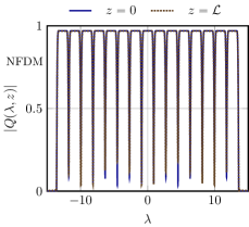
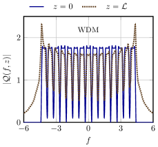
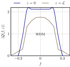
      (a)      (b)      (c)

Figure 6: Interference in WDM and NFDM in the absence of noise, for signals with the same power, bandwidth and time duration. (a) No interference in NFDM. Interference in WDM: (b) before equalization, and (c) after equalization.

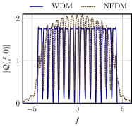
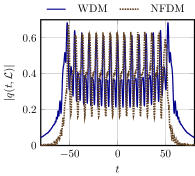
      (a)        (b)

Figure 7: WMD and NFDM signals have the same (a) bandwidth $B=60$ GHz (that is maximum at $z=0$), and (b) time duration 1.5 ns (that is maximum at $z=2000$ km). The power is ${\mathcal{P}}=0$ dBm.

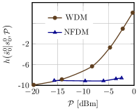
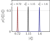
      (a)      (b)

Figure 8: (a) Compared with WDM, the conditional differential entropy in NFDM is nearly constant as ${\mathcal{P}}$ is increased ($s_{0}^{0}=0.2$). (b) The conditional probability distribution $p\bigl{(}|\hat{s}_{0}^{0}|\bigl{|}s_{0}^{0}\bigr{)}$ in NFDM, for three values of $s_{0}^{0}$.

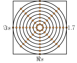
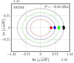
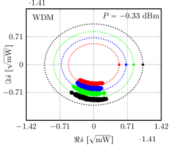
(a)	(b)	(c)

Figure 9: (a) Constellation for $s_{\ell}^{k}$ in the $U$ domain. Received symbols for four transmitted symbols in (b) NFDM, and (c) WDM.

VIII Conclusion

The paper shows that the NFDM AIR is greater than the WDM AIR for a given power and bandwidth, in an integrable model of the optical fiber in the defocusing regime, and in a representative system with one symbol per user. While the paper serves as a good starting point, more research is needed in comparing the linear and nonlinear multiplexing.

Acknowledgments

The research was done when the authors were at TU Munich in Germany. Financial support of the Institute for Advanced Study at TU Munich, funded by the German Excellence Initiative, as well as Alexander von Humboldt Foundation, funded by the German Federal Ministry of Education and Research, is acknowledged. Mansoor Yousefi benefited from discussions with Frank Kschischang and Gerhard Kramer.

Appendix A Proof of (38) and (42)

The first few iterations in the scaled AL scheme are:

$$\begin{pmatrix}A[0,z]\\ B[0,z]\end{pmatrix} = \begin{pmatrix}1\\ 0\end{pmatrix},\quad\begin{pmatrix}A[1,z]\\ B[1,z]\end{pmatrix}=\bar{c}_{0}\begin{pmatrix}1\\ sQ^{*}_{0}\end{pmatrix},$$

$$\begin{pmatrix}A[2,z]\\ B[2,z]\end{pmatrix} = \bar{c}_{1}\begin{pmatrix}1+sQ^{*}_{0}Q_{1}z^{-1}\\ sQ^{*}_{1}+sQ^{*}_{0}z^{-1}\end{pmatrix},$$

$$\begin{pmatrix}A[3,z]\\ B[3,z]\end{pmatrix} = \bar{c}_{2}\begin{pmatrix}1+s(Q^{*}_{0}Q_{0}+Q^{*}_{1}Q_{2})z^{-1}+sQ^{*}_{0}Q_{2}z^{-2}\\ sQ^{*}_{2}-s(Q^{*}_{0}Q_{1}Q^{*}_{2}-Q^{*}_{1})z^{-1}+sQ^{*}_{0}z^{-2}\end{pmatrix},$$

where $Q_{k}\stackrel{{\scriptstyle\Delta}}{{=}}Q[k]$ and $\bar{c}_{k}\stackrel{{\scriptstyle\Delta}}{{=}}\prod_{i=0}^{k}c_{i}$.

For $k=0,1,2$, the coefficients of $A[k+1,z]$ and $B[k+1,z]$ with the smallest power of $z^{-1}$ are

$$A_{0}[k+1]=\bar{c}_{k},\quad B_{0}[k+1]=s\bar{c}_{k}Q^{*}[k].$$ (53)

By induction, (53) holds for all $k\geq 0$. Thus, $Q^{*}[k]=sB_{0}[k+1]/A_{0}[k+1]$, which is (38).

Similarly, for $k=1,2$, the coefficients of $A[k+1,z]$ and $B[k+1,z]$ with the highest power of $z^{-1}$ are

$$A_{k}[k+1]=s\bar{c}_{k}Q_{0}^{*}Q_{k},\quad B_{k}[k+1]=s\bar{c}_{k}Q^{*}_{0}.$$

By induction, the last equation holds for all $k\geq 1$. Thus, $Q[k]=A_{k}[k+1]/B_{k}[k+1]$, which is (42).

Appendix B Kramers-Kronig Relations

The real and imaginary parts of an analytic function are related via the Kramers-Kronig relations.

Lemma 1 (Kramers-Kronig Relations).

Let $f(z)\stackrel{{\scriptstyle\Delta}}{{=}}u(x,y)+jv(x,y)$ be a function of a complex variable $z\stackrel{{\scriptstyle\Delta}}{{=}}x+jy\in\mathbb{C}^{+}$, where $u$ and $v$ are real-valued functions. Suppose that $f(z)$ is analytic in $\mathbb{C}^{+}$ and $f(z)$ decays as $1/z$ as $|z|\rightarrow\infty$. Then

$$u(x,y)=-\mathcal{H}_{x}(v(x,y)),\quad v(x,y)=\mathcal{H}_{x}(u(x,y)),$$ (54)

where $\mathcal{H}_{x}$ denotes the Hilbert transform with respect to $x$:

$$\mathcal{H}_{x}(f(x,y)) \stackrel{{\scriptstyle\Delta}}{{=}} \frac{1}{\pi}\textnormal{p.v.}\int\limits_{-\infty}^{\infty}\frac{f(x^{\prime},y)}{x-x^{\prime}}\mathrm{d}x^{\prime}$$

$$= \frac{1}{\pi x}\convolution f(x,y),$$

where $\convolution$ is convolution with respect to $x$, and p.v. is the principal value.

Proof.

The result follows immediately from the Cauchy’s integral formula, or the Sokhotski-Plemelj formula [1, Lem. 8].

∎

Lemma 2.

Let $q(t)\in L^{1}(\mathbb{R})$ and $a(\lambda)$ be the corresponding nonlinear Fourier coefficient in the defocusing regime. Then

$${\rm{Arg}}(a(\lambda))=\mathcal{H}(\log|a(\lambda)|),$$ (55)

for all $\lambda\in\mathbb{R}$ for which ${\rm{Arg}}(a(\lambda))\in(-\pi,\pi)$.

∎

Proof.

If $q(t)\in L^{1}(\mathbb{R})$ and $s=1$, $a(\lambda)$ can be analytically extended to $\mathbb{C}^{+}$ and is continuous in $\bar{\mathbb{C}}^{+}\stackrel{{\scriptstyle\Delta}}{{=}}\bigl{\{}\lambda\in\mathbb{C}:\Im(\lambda)\geq 0\bigr{\}}$ [6, Lemma 2.1], [1, Lem. 4]. Consider the open region $\mathcal{D}\stackrel{{\scriptstyle\Delta}}{{=}}\{\lambda\in\mathbb{C}:0<\Im(\lambda)<\epsilon\}$ with $\epsilon\rightarrow 0^{+}$. Note $a(\lambda)$ is analytic on $\mathcal{D}$ and continuous on its closure $\bar{\mathcal{D}}$. From the unimodularity condition (15) with $s=1$

$$|a|^{2} = 1+|b|^{2}$$

$$\geq 1,\quad\lambda\in\mathbb{R},$$

thus $|a(\lambda)|\neq 0$ for $\lambda\in\mathbb{R}$. Because $a(\lambda)$ is continuous on $\bar{\mathcal{D}}$, we obtain $a(\lambda)\neq 0$ on $\bar{\mathcal{D}}$ (recall $\epsilon\rightarrow 0$). Taking the principal branch of the logarithm, function $\lambda\mapsto\log(\lambda)$ is continuous in $\mathbb{C}\backslash\{0\}$ and analytic on $\mathbb{C}\backslash\mathbb{R}_{0}^{-}$, where $\mathbb{R}_{0}^{-}$ is a branch cut of the logarithm. Since $a(\lambda)$ is analytic and non-zero on $\mathcal{D}$, and $\textnormal{range}(a(\lambda))\subseteq\mathbb{C}\backslash\mathbb{R}_{0}^{-}$, $\log a(\lambda)$ is analytic on $\mathcal{D}$, and continuous on $\bar{\mathcal{D}}$.

We next show that $\log a(\lambda)$ satisfies the decay assumption in Lemma 1. From [1, Eq. 45],

$$a(\lambda)=1-\frac{jE}{2}\lambda^{-1}+\mathcal{O}(\lambda^{-2}),\quad\textnormal{as}\quad|\lambda|\rightarrow\infty,$$

where $E\stackrel{{\scriptstyle\Delta}}{{=}}\int\limits_{-\infty}^{\infty}|q(t)|^{2}\mathrm{d}t$. Thus

$$|\log a(\lambda)|\rightarrow 0.5E\lambda^{-1},\quad\textnormal{as},\quad|\lambda|\rightarrow\infty.$$ (56)

Applying Lemma 1 on $\mathcal{D}$ gives

$${\rm{Arg}}(a(\lambda))=\mathcal{H}(\log|a(\lambda)|),\quad\lambda\in\mathcal{D}.$$ (57)

We show (57) holds for $\lambda\in\mathbb{R}$ using continuity. For $x\in\mathbb{R}$

$${\rm{Arg}}(a(x)) = {\rm{Arg}}\bigl{(}a(\lim\limits_{\epsilon\rightarrow 0^{+}}(x+j\epsilon))\bigr{)}$$

$$\overset{(a)}{=} {\rm{Arg}}\bigl{(}\lim\limits_{\epsilon\rightarrow 0^{+}}a(x+j\epsilon)\bigr{)}$$

$$\overset{(b)}{=} \lim\limits_{\epsilon\rightarrow 0^{+}}{\rm{Arg}}(a(x+j\epsilon))$$

$$\overset{(c)}{=} œ\lim\limits_{\epsilon\rightarrow 0^{+}}\mathcal{H}\bigl{(}\log|a(x+j\epsilon)|\bigr{)}$$

$$\overset{(d)}{=} \mathcal{H}\Bigl{(}\lim\limits_{\epsilon\rightarrow 0^{+}}\log|a(x+j\epsilon)|\Bigr{)}$$

$$\overset{(e)}{=} \mathcal{H}(\log|a(x)|).$$

Step $(a)$ follows because $a(\lambda)$ is continuous in $\bar{\mathcal{D}}$. Step $(b)$ follows because $a(\lambda)$ is continuous and non-zero in $\bar{\mathcal{D}}$, and $\lambda\mapsto\log(\lambda)$ is continuous in $\mathbb{C}\backslash\{0\}$, thus ${\rm{Arg}}(a)\in(-\pi,\pi)$ is continuous in its principal branch. Step $(c)$ follows from (57). Step $(d)$ holds because $\mathcal{H}$ is a continuous operator on the space of functions $\log|a(\lambda)|$, as we show below. Step $(e)$ holds because $\log|a(\lambda)|$ is continuous on $\bar{\mathcal{D}}$.

We show that the order of the limit and the integral can be exchanged in the following Hilbert transform:

$${\rm{Arg}}(a(x))=\frac{1}{\pi}\lim\limits_{\epsilon\rightarrow 0^{+}}\textnormal{p.v.}\int\limits_{-\infty}^{\infty}\frac{\log|a(x^{\prime}+j\epsilon)|}{x-x^{\prime}}\mathrm{d}x^{\prime}.$$

Let $\delta>0$ be sufficiently small and $K<\infty$ sufficiently large. We partition the integration range into the union of $I_{0}\stackrel{{\scriptstyle\Delta}}{{=}}\{x^{\prime}:|x^{\prime}-x|<\delta\}$, $I_{1}\stackrel{{\scriptstyle\Delta}}{{=}}\{x^{\prime}:|x^{\prime}|\leq K,\>x^{\prime}\notin I_{0}\}$ and $I_{2}\stackrel{{\scriptstyle\Delta}}{{=}}\{x^{\prime}:|x^{\prime}|>K\}$. From (56), there exists $C_{2}<\infty$ such that

$$\left|\frac{\log|a(x^{\prime}+j\epsilon)|}{x^{\prime}-x}\right|<\frac{C_{2}}{|x^{\prime}(x^{\prime}-x)|},\quad x^{\prime}\in I_{2}.$$ (58)

The right hand side in (58) is independent of $\epsilon$ and integrable for $x^{\prime}\in I_{2}$. Likewise, because $a(\lambda)$ is continuous on $\bar{\mathcal{D}}$ and $I_{1}$ is compact, from the extreme value theorem $|a(x^{\prime}+j\epsilon)|<C_{1}$ for $x^{\prime}\in I_{1}$ and some $C_{1}<\infty$, independently of $\epsilon$. Thus the integrand corresponding to $I_{1}$ is uniformly upper bounded by an absolutely integrable function. Consequently, from the dominated convergence theorem the order of the limit and the integral can be exchanged in integrals over $I_{1}$ and $I_{2}$. Finally, since $\log|a(\lambda)|$ is continuous, the integral over $I_{0}$ evaluates to $\log|a(x)|\times\textnormal{p.v.}\int_{-\delta}^{\delta}\frac{1}{x}\mathrm{d}x=0$.

∎

Remark 3.

If $q(t)\in L^{1}(\mathbb{R})$, $a(\lambda)$ is analytic on $\mathbb{C}^{+}$, but not necessarily on $\bar{\mathbb{C}}^{+}$, unless $q(t)$ vanishes exponentially as $t\rightarrow\pm\infty$. For such signals, $\log a(\lambda)$ is analytic on $\bar{\mathbb{C}}^{+}$, and the proof of Lemma 2 simplifies.

∎

References

- [1] M. I. Yousefi and F. R. Kschischang, “Information transmission using the nonlinear Fourier transform, Part I: Mathematical tools,” IEEE Trans. Inf. Theory, vol. 60, no. 7, pp. 4312–4328, Jul. 2014.
- [2] ——, “Information transmission using the nonlinear Fourier transform, Part II: Numerical methods,” IEEE Trans. Inf. Theory, vol. 60, no. 7, pp. 4329–4345, Jul. 2014.
- [3] ——, “Information transmission using the nonlinear Fourier transform, Part III: Spectrum modulation,” IEEE Trans. Inf. Theory, vol. 60, no. 7, pp. 4346–4369, Jul. 2014.
- [4] M. I. Yousefi, “Information transmission using the nonlinear Fourier transform,” Ph.D. dissertation, University of Toronto, Mar. 2013.
- [5] G. Boffetta and A. R. Osborne, “Computation of the direct scattering transform for the nonlinear Schrödinger equation,” J. Comp. Phys., vol. 102, no. 2, pp. 252–264, Oct. 1992.
- [6] M. J. Ablowitz, B. Prinari, and A. D. Trubatch, Discrete and Continuous Nonlinear Schrödinger Systems, 1st ed., ser. Lond. Math. Soc. Lec. Note Series. Cambridge, UK: Cambridge University Press, 2003, vol. 302.
- [7] M. I. Yousefi, “The Kolmogorov-Zakharov model for optical fiber communication,” IEEE Trans. Inf. Theory, vol. 61, no. 1, pp. 377–391, Jan. 2017.
- [8] A. Hasegawa and T. Nyu, “Eigenvalue communication,” IEEE J. Lightw. Technol., vol. 11, no. 3, pp. 395–399, Mar. 1993.
- [9] E. Meron, M. Feder, and M. Shtaif, “On the achievable communication rates of generalized soliton transmission systems,” Arxiv peprint, arXiv:1207.0297, pp. 1–13, Jul. 2012.
- [10] J. E. Prilepsky, S. A. Derevyanko, K. J. Bluw, I. Gabitov, and S. K. Turitsyn, “Nonlinear inverse synthesis and eigenvalue division multiplexing in optical fiber channels,” Phys. Rev. Lett., vol. 113, no. 1, pp. 013 901 (1–5), Jul. 2014.
- [11] S. Hari, M. I. Yousefi, and F. R. Kschischang, “Multieigenvalue communication,” IEEE J. Lightw. Technol., vol. 34, no. 13, pp. 3110–3117, Jul. 2016.
- [12] Z. Dong, S. Hari, T. Gui, K. Zhong, M. I. Yousefi, C. Lu, P.-K. A. Wai, F. R. Kschischang, and A. P. T. Lau, “Nonlinear frequency division multiplexed transmissions based on NFT,” IEEE Photon. Technol. Lett., vol. 27, no. 15, pp. 1621–1623, Aug. 2015.
- [13] R. G. Gallager, Principles of Digital Communication. Cambridge, UK: Cambridge University Press, 2008.
- [14] S. T. Le, J. E. Prilepsky, and S. K. Turitsyn, “Nonlinear inverse synthesis for high spectral efficiency transmission in optical fibers,” Opt. Exp., vol. 22, no. 22, pp. 26 720–26 741, Nov. 2014.
- [15] S. T. Le, S. Wahls, D. Lavery, J. E. Prilepsky, and S. K. Turitsyn, “Reduced complexity nonlinear inverse synthesis for nonlinearity compensation in optical fiber links,” in The European Conf. Lasers Electro-Optics, Munich, Germany, Jun. 2015.
- [16] H. Bülow, V. Aref, and L. Schmalen, “Modulation on discrete nonlinear spectrum: Perturbation sensitivity and achievable rates,” IEEE Photon. Technol. Lett., vol. 30, no. 5, pp. 423 –426, Mar. 2018.
- [17] H. Buelow, V. Aref, and W. Idler, “Transmission of waveforms determined by 7 eigenvalues with PSK-modulated spectral amplitudes,” in European Conf. on Opt. Commun., Düsseldorf, Germany, Sep. 2016, pp. 1–3.
- [18] V. Aref, H. Buelow, K. Schuh, and W. Idler, “Experimental demonstration of nonlinear frequency division multiplexed transmission,” in European Conf. Opt. Commun., Valencia, Spain, Sep. 2015, pp. 1–3.
- [19] V. Aref, “Control and detection of discrete spectral amplitudes in nonlinear Fourier spectrum,” arXiv: 1605.06328, May 2016.
- [20] H. Terauchi and A. Maruta, “Eigenvalue modulated optical transmission system based on digital coherent technology,” in Joint OptoElec. Commun. Conf. & 2013 Int. Conf. Photonics in Switching (OECC/PS), Kyoto, Japan, Jul. 2013, pp. 1–2.
- [21] A. Span, V. Aref, H. Bülow, and S. T. Brink, “On time-bandwidth product of multi-soliton pulses,” in IEEE Int. Symp. Info. Theory, Aachen, Germany, Jun. 2017, pp. 61–65.
- [22] W. Q. Zhang et al., “Correlated eigenvalues optical communications,” Arxiv preprints, arxiv:1711.09227, pp. 1–14, Nov. 2017.
- [23] J. Garcia, “Communication using eigenvalues of higher multiplicity of the nonlinear Fourier transform,” ArXiv preprint, arxiv:1802.07456, pp. 1–8, Feb. 2018.
- [24] V. Aref, S. T. Le, and H. Buelow, “Demonstration of fully nonlinear spectrum modulated system in the highly nonlinear optical transmission regime,” in European Conf. on Opt. Commun., Düsseldorf, Germany, Sep. 2016, pp. 1–3.
- [25] I. Tavakkolnia and M. Safari, “Signalling over nonlinear fibre-optic channels by utilizing both solitonic and radiative spectra,” in European Conf. Networks and Commun., Paris, France, Jul. 2015, pp. 103–107.
- [26] V. Aref, S. T. Le, and H. Buelow, “Modulation over nonlinear fourier spectrum: Continuous and discrete spectrum,” IEEE J. Lightw. Technol., vol. 36, no. 6, pp. 1289–1295, Mar. 2018.
- [27] Q. Zhang and T. H. Chan, “A spectral domain noise model for optical fibre channels,” in IEEE Int. Symp. Info. Theory, Hong Kong, Jun. 2015, pp. 1660–1664.
- [28] Q. Zhang, T. H. Chan, and A. Grant, “Spatially periodic signals for fiber channels,” in IEEE Int. Symp. Info. Theory, Honolulu, HI, USA, Jun. 2014, pp. 2804–2808.
- [29] S. Civelli, E. Forestieri, and M. Secondini, “Decision-feedback detection strategy for nonlinear frequency-division multiplexing,” arXiv preprint, arxiv:1801.05338, 2018.
- [30] ——, “A novel detection strategy for nonlinear frequency-division multiplexing,” in Opt. Fiber Commun. Conf., San Diego, CA, USA, Mar. 2018, pp. 1–3.
- [31] P. Kazakopoulos and A. L. Moustakas, “Nonlinear Schrödinger equation with random Gaussian input: Distribution of inverse scattering data and eigenvalues,” Phys. Rev. E, vol. 78, no. 1, pp. 016 603 (1–7), Jul. 2008.
- [32] S. Civelli, E. Forestieri, and M. Secondini, “Why noise and dispersion may seriously hamper nonlinear frequency-division multiplexing,” IEEE Photon. Technol. Lett., vol. 29, no. 16, pp. 1332–1335, Aug. 2017.
- [33] X. Yangzhang, D. Lavery, P. Bayvel, and M. I. Yousefi, “Impact of perturbations on nonlinear frequency-division multiplexing,” IEEE J. Lightw. Technol., vol. 36, no. 2, pp. 485–494, Jan. 2018.
- [34] V. Aref, S. T. Le, and H. Bülow, “Does the cross-talk between nonlinear modes limit the performance of NFDM systems?” in European Conf. on Opt. Commun., Sep. 2017, pp. 1–3.
- [35] R. T. Jones, S. Gaiarin, M. P. Yankov, and D. Zibar, “Noise robust receiver for eigenvalue communication systems,” in Opt. Fiber Commun. Conf., San Diego, CA, USA, Mar. 2018, pp. W2A–59.
- [36] A. M. Bruckstein, B. C. Levy, and T. Kailath, “Differential methods in inverse scattering,” SIAM J. Appl. Math., vol. 45, no. 2, pp. 312–335, Apr. 1985.
- [37] J. Skaar and O. H. Waagaard, “Design and characterization of finite-length fiber gratings,” IEEE J. Quantum Electron., vol. 39, no. 10, pp. 1238–1245, Oct. 2003.
- [38] A. Rosenthal and M. Horowitz, “Inverse scattering algorithm for reconstructing strongly reflecting fiber Bragg gratings,” IEEE J. Quantum Electron., vol. 39, no. 8, pp. 1018–1026, Aug. 2003.
- [39] A. Buryak, J. Bland-Hawthorn, and V. Steblina, “Comparison of inverse scattering algorithms for designing ultrabroadband fibre bragg gratings,” Opt. Exp., vol. 17, no. 3, pp. 1995–2004, Feb. 2009.
- [40] S. Civelli, L. Barletti, and M. Secondini, “Numerical methods for the inverse nonlinear Fourier transform,” in Tyrrhenian Int. Workshop on Digital Commun., Florence, Italy, Sep. 2015, pp. 13–16.
- [41] S. Wahls and H. V. Poor, “Fast numerical nonlinear Fourier transforms,” IEEE Trans. Inf. Theory, vol. 61, no. 12, pp. 6957–6974, Dec. 2015.
- [42] ——, “Fast inverse nonlinear Fourier transform for generating multi-solitons in optical fiber,” in IEEE Int. Symp. Info. Theory, Hong Kong, China, Jun. 2015, pp. 1676–1680.
- [43] S. Wahls, S. T. Le, J. E. Prilepsky, H. V. Poor, and S. K. Turitsyn, “Digital backpropagation in the nonlinear Fourier domain,” in IEEE Int. Workshop Signal Process. Advances Wireless Commun., Stockholm, Sweden, Jun. 2015, pp. 445–449.
- [44] V. Vaibhav, “Fast inverse nonlinear Fourier transform,” ArXiv preprint, arxiv:1706.04069, Jun. 2017.
- [45] S. Gaiarin, A. M. Perego, E. P. da Silva, F. D. Ros, and D. Zibar, “Experimental demonstration of dual polarization nonlinear frequency division multiplexed optical transmission system,” in European Conf. on Opt. Commun., Gothenburg, Sweden, Sep. 2017, pp. 1–3.
- [46] S. Gaiarin, A. M. Perego, E. P. da Silva, F. Da Ros, and D. Zibar, “Dual-polarization nonlinear Fourier transform-based optical communication system,” Optica, vol. 5, no. 3, pp. 263–270, Mar. 2018.
- [47] J.-W. Goossens, M. I. Yousefi, Y. Jaouën, and H. Hafermann, “Polarization-division multiplexing based on the nonlinear Fourier transform,” Opt. Exp., vol. 25, no. 22, pp. 26 437–26 452, Oct. 2017.
- [48] M. Kamalian, J. E. Prilepski, S. T. Le, and S. Turitsyn, “Periodic nonlinear Fourier transform for fiber-optic communications, Part I–II,” Opt. Exp., vol. 24, no. 16, pp. 18 353–18 381, Aug. 2016.
- [49] N. A. Shevchenko et al., “A lower bound on the per soliton capacity of the nonlinear optical fibre channel,” in IEEE Info. Theory Workshop, Jeju Island, South Korea, Oct. 2015, pp. 1–5.
- [50] P. Kazakopoulos and A. L. Moustakas, “On the soliton spectral efficiency in non-linear optical fibers,” in IEEE Int. Symp. Info. Theory, Barcelona, Spain, Jul. 2016, pp. 610–614.
- [51] I. Tavakkolnia and M. Safari, “Capacity analysis of signaling on the continuous spectrum of nonlinear optical fibers,” IEEE J. Lightw. Technol., vol. 35, no. 11, pp. 2086–2097, Jun. 2017.
- [52] S. A. Derevyanko, J. E. Prilepsky, and S. K. Turitsyn, “Capacity estimates for optical transmission based on the nonlinear Fourier transform,” Nature Commun., vol. 7, no. 12710, pp. 1–9, Sep. 2016.
- [53] ——, “Capacity estimates for optical transmission based on the nonlinear fourier transform,” Nature Commun., vol. 7, Sep. 2016, Paper no. 12710.
- [54] P. Kazakopoulos and A. L. Moustakas, “On the soliton spectral efficiency in non-linear optical fibers,” in IEEE Int. Symp. Info. Theory, Barcelona, Spain, Jul. 2016, pp. 610–614.
- [55] H. Bülow, “Nonlinear Fourier transformation based coherent detection scheme for discrete spectrum,” in Opt. Fiber Commun. Conf. and Exposition, Los Angeles, CA, USA, Mar. 2015, pp. 1–3.
- [56] ——, “Experimental assessment of nonlinear Fourier transformation based detection under fiber nonlinearity,” in European Conf. Opt. Commun., Cannes, France, Sep. 2014, pp. 1–3.
- [57] H. Bülow, “Experimental demonstration of optical signal detection using nonlinear Fourier transform,” IEEE J. Lightw. Technol., vol. 33, no. 7, pp. 1433–1439, Apr. 2015.
- [58] A. Maruta, A. Toyota, Y. Matsuda, and Y. Ikeda, “Experimental demonstration of long haul transmission of eigenvalue modulated signals,” in Tyrrhenian Int. Workshop on Digital Commun., Sep. 2015, pp. 28–30.
- [59] T. Gui et al., “Polarization-division-multiplexed nonlinear frequency division multiplexing,” in The Conf. Lasers Electro-Optics, San Jose, CA, USA, May 2018, pp. 1–2.
- [60] S. T. Le, H. Buelow, and V. Aref, “Demonstration of 64 0.5 Gbaud nonlinear frequency division multiplexed transmission with 32QAM,” in Opt. Fiber Commun. Conf., Los Angeles, CA, USA, Mar. 2017, pp. 1–3.
- [61] S. T. Le, V. Aref, and H. Buelow, “High speed precompensated nonlinear frequency-division multiplexed transmissions,” IEEE J. Lightw. Technol., vol. 36, no. 6, pp. 1296–1303, Mar. 2018.
- [62] X. Yangzhang, M. I. Yousefi, A. Alvarado, D. Lavery, and P. Bayvel, “Nonlinear frequency-division multiplexing in the focusing regime,” in Opt. Fiber Commun. Conf., Los Angeles, USA, Mar. 2017, pp. 1–3.
- [63] G. P. Agrawal, Nonlinear Fiber Optics, 4th ed. San Francisco, CA, USA: Academic, 2007.
- [64] A. Splett, C. Kurtzke, and K. Petermann, “Ultimate transmission capacity of amplified optical fiber communication systems taking into account fiber nonlinearities,” in European Conf. Opt. Commun., Montreux, Switzerland, Sep 1993, pp. 41–44.
- [65] R. J. Essiambre, G. Kramer, P. J. Winzer, G. J. Foschini, and B. Goebel, “Capacity limits of optical fiber networks,” IEEE J. Lightw. Technol., vol. 28, no. 4, pp. 662–701, Feb. 2010.
- [66] E. Agrell, “Conditions for a monotonic channel capacity,” IEEE Trans. Commun., vol. 63, no. 3, pp. 1–11, Sep. 2015.
- [67] J. Tang, “The Shannon channel capacity of dispersion-free nonlinear optical fiber transmission,” IEEE J. Lightw. Technol., vol. 19, no. 8, pp. 1104–1109, Aug. 2001.
- [68] G. D. Forney, Jr., “Principles of digital communication II.” Massachusetts Institute of Technology, Mar. 2005, MIT OpenCourseWare, Course no. 6.451, Lecture Notes.
- [69] M. I. Yousefi, “The asymptotic capacity of the optical fiber,” Arxiv preprint, arXiv:1610.06458, pp. 1–12, Nov. 2016.