MINLP in Transmission Expansion Planning

Abstract

Transmission expansion planning requires forecasts of demand for electric power and a model of the underlying physics, i.e., power flows. We present three approaches to deriving exact solutions to the transmission expansion planning problem in the alternating-current model, for a given load.

I Introduction

Consider the problem of optimal investment in line capacity, such that a sum of annualised investment costs and an estimate of operational costs is minimised. The estimate of operational costs and its computational complexity depend on the model of power flows used. Considering the recent progress in the development of convergent solvers for polynomial optimisation [1], we explore the options for solving the transmission expansion problem exactly in the alternating-current model.

This is motivated by the observation [2] that the quality of the approximation of the alternating-current model has a major impact on the investment decisions. Specifically, the use of the simplistic direct-current approximation (DCOPF) may result in no lines being built. Various piece-wise linearisations may result in various lines being built, other than those built considering the alternating-current model (ACOPF) proper. This is the case even when loads are known exactly, i.e., independently of the uncertainty in the load.

We compare three convergent approaches to solving the transmission expansion planning problem in the alternating-current model. First, we study both the current-voltage (IV) and power-voltage (PQV) formulations of the problem as polynomial optimisation problems and derive semidefinite-programming relaxations (SDP) thereof using the techniques of [1]. Second, we introduce a novel lift-and-branch-and-bound procedure using SDP relaxations we introduce, which makes it possible to obtain global optima for small instances of the transmission expansion problem. Finally, we compare these approaches with state-of-the-art piece-wise linearisations based on the current-voltage formulation and a rudimentary DCOPF approximation. Although we do not consider multiple scenarios for the demand, it would be easy to extend the work in the direction of two-stage or multi-stage stochastic programming.

II The Problem

Formally, let introduce the problem using:

• $(\mathcal{N},\mathcal{A})$ be the graph representing an electrical network with buses $\mathcal{N}$ and lines $\mathcal{A}$

• $p_{i}+\mathbf{j}q_{i}$ be the complex net power injection at bus $i\in\mathcal{N}$,

• $z_{i}+\mathbf{j}w_{i}$ be the complex net current injected at bus $i\in\mathcal{N}$,

• $z_{ij}+\mathbf{j}w_{ij}$ be the complex current flow on line $(i,j)\in\mathcal{A}$ (with slight abuse of notation), and let

• $v_{i}+\mathbf{j}u_{i}$ be the complex voltage at bus $i\in\mathcal{N}$ and

• $o_{ij}=1$ if circuit $(i,j)\in\mathcal{A}$ is open and 0 otherwise.

The transmission expansion problem may be stated as follows:

$$\min c^{\top}p$$ [IV]

s.t. $$z_{i}+\sum_{j\in\mathcal{N}}(z_{ji}-z_{ij})=0 \forall i\in\mathcal{N}$$ (1)

$$w_{i}+\sum_{j\in\mathcal{N}}(w_{ji}-w_{ij})=0 \forall i\in\mathcal{N}$$ (2)

$$\uline{p}_{i}\leq p_{i}=v_{i}z_{i}+u_{i}w_{i}\leq\bar{p}_{i} \forall i\in\mathcal{N}$$ (3)

$$\uline{q}_{i}\leq q_{i}=u_{i}z_{i}-v_{i}w_{i}\leq\bar{q}_{i} \forall i\in\mathcal{N}$$ (4)

$$\uline{v}_{i}^{2}\leq v_{i}^{2}+u_{i}^{2}\leq\bar{v}_{i}^{2} \forall i\in\mathcal{N}$$ (5)

$$o_{ji}\in\{0,1\} \forall(i,j)\in A$$ (6)

$$o_{ij}=0\Rightarrow v_{i}-v_{j}=R_{ij}z_{ij}-X_{ij}w_{ij} \forall(i,j)\in\mathcal{A}$$ (7)

$$o_{ij}=0\Rightarrow u_{i}-u_{j}=X_{ij}z_{ij}+R_{ij}w_{ij} \forall(i,j)\in\mathcal{A}$$ (8)

$$o_{ij}=0\Rightarrow z_{ij}^{2}+w_{ij}^{2}\leq\bar{z}_{ij}^{2} \forall(i,j)\in\mathcal{A}$$ (9)

$$o_{ij}=1\Rightarrow z_{ij}^{2}+w_{ij}^{2}\leq 0 \forall(i,j)\in\mathcal{A}$$ (10)

where:

• $c$ denotes the vector of generator marginal costs, which are assumed to be known ans constant, for simplicity,

• $R_{ij}$ and $X_{ij}$ denote the resistance and reactance respectively of line $(i,j)$.

• $\uline{p}$ and $\bar{p}$ denote minimum active power generation and capacity vectors,

• $\uline{q}$ and $\bar{q}$ denote minimum reactive power generation and capacity vectors,

• $\uline{v}$ and $\bar{v}$ denote vectors of minimum and maximum voltage magnitudes, and

• $\bar{z}$ is the thermal capacity limit of lines.

III A Piece-Wise Linearisation

Several authors have proposed piece-wise linearisations of the current-voltage formulation of optimal power flows (ACOPF-IV) and related problems, which yield mixed-integer linear programming formulations [3, 4, 5, 6, 7]. The idea of piece-wise linearisation is well-known and often very efficient. Most of the proposed piece-wise linearisations, e.g. [4, 2, 7], however, cannot reach the global optimum in the limit of the number of segments, due to the additional assumptions surveyed in Table 1 of [7]. In the following, we extend the formulation proposed in [6] to accommodate dispatch of real and reactive power, and hence obtain a “principled” piece-wise linearisation.

The upper bound on voltage magnitude in (5) are convex quadratic constraints, that may be replaced by an outer linear approximation as in [5]. The remaining non-linear constraints (3), (4), and the first inequality of (5) is discussed below.

In general, the complex current injection may be written in terms of voltage and power as

$$I=z+\mathbf{j}w=\frac{S}{V}=\frac{p+\mathbf{j}q}{v+\mathbf{j}u}=\frac{vp+uq}{v^{2}+u^{2}}+\mathbf{j}\frac{vq-up}{v^{2}+u^{2}}$$

By employing a discretisation of the complex two-dimensional $(V,S)$-space, we can linearise the complex current injection. We propose to discretise the complex voltage space $V$ along its polar coordinates, while discretising the power along rectangular coordinates. This ensures a tight approximation to the feasible area of the voltage space. Let $\hat{|V|}$, $\hat{\theta}$, $\hat{p}$, and $\hat{q}$ be the vectors of values at the discretisation points in the four real dimensions, voltage magnitude, voltage angle, real, and reactive power, respectively. We then evaluate the value of the current injection in each of the $|\hat{|V|}|\times|\hat{\theta}|\times|\hat{p}|\times|\hat{q}|$ discretisation points as $\hat{z}+\mathbf{j}\hat{w}$.

Now, at any point in the $(|V|,\theta,p,q)$-space we can approximate all relevant quantities as a convex combination $\lambda$ of the values in the immediately surrounding discretisation points. That is, for all $i\in\mathcal{N}$

$$v_{i} =\sum_{j,k,l,m}\hat{|V|}_{i}^{j}\cos\hat{\theta}_{i}^{k}\lambda_{i}^{jklm} u_{i} =\sum_{j,k,l,m}\hat{|V|}_{i}^{j}\sin\hat{\theta}_{i}^{k}\lambda_{i}^{jklm}$$

$$p_{i} =\sum_{j,k,l,m}\hat{p}_{i}^{l}\lambda_{i}^{jklm} q_{i} =\sum_{j,k,l,m}\hat{q}_{i}^{m}\lambda_{i}^{jklm}$$

$$z_{i} =\sum_{j,k,l,m}\hat{z}_{i}^{jklm}\lambda_{i}^{jklm} w_{i} =\sum_{j,k,l,m}\hat{w}_{i}^{jklm}\lambda_{i}^{jklm}$$

$$|V_{i}| =\sum_{j,k,l,m}\hat{|V|}_{i}^{j}\lambda_{i}^{jklm}$$

In each dimension we choose a convex combination of discretisation points,

$$\sum_{j\in\mathcal{J}}\sum_{k\in\mathcal{K}}\sum_{l\in\mathcal{L}}\sum_{m\in\mathcal{M}}\lambda_{i}^{jklm}=1\quad\forall i\in\mathcal{N}$$

with $\lambda_{i}^{jklm}\geq 0$ for all $i\in\mathcal{N},j\in\mathcal{J},k\in\mathcal{K},l\in\mathcal{L},m\in\mathcal{M}$. The so called “special ordered set of type 2” (SOS2) constraints ensures that we choose a combination of the two closest discretisation points in each dimension:

$$\lambda^{jklm} \leq\psi^{j-1}+\psi^{j},\forall j\in\mathcal{J}\setminus\{0\}$$

$$\lambda^{jklm} \leq\chi^{k-1}+\chi^{k},\forall k\in\mathcal{K}\setminus\{0\}$$

$$\lambda^{jklm} \leq\varphi^{l-1}+\varphi^{l},\forall l\in\mathcal{L}\setminus\{0\}$$

$$\lambda^{jklm} \leq\upsilon^{m-1}+\upsilon^{m},\forall m\in\mathcal{M}\setminus\{0\}$$

$$\lambda^{j,0,0,0} \leq\psi^{0} \lambda^{0,k,0,0} \leq\chi^{0}$$

$$\lambda^{0,0,l,0} \leq\varphi^{0} \lambda^{0,0,0,m} \leq\upsilon^{0}$$

$$e^{\top}\psi =e^{\top}\chi=e^{\top}\varphi=e^{\top}\upsilon=1 \psi,\chi,\varphi,\upsilon \in\{0,1\}$$

where $\mathcal{J},\mathcal{K},\mathcal{L}$, and $\mathcal{M}$ are the index sets of the discretisation points $\hat{|V|},\hat{\theta}$, and $\hat{p}$ $\hat{q}$, respectively. That is,

• $\psi^{j}=1$ if and only if $V$ is in the interval $\left[\hat{|V|}^{j},\hat{|V|}^{j+1}\right]$,

• $\chi^{k}=1$ if and only if $\theta$ is in the interval $\left[\hat{\theta}^{k},\hat{\theta}^{k+1}\right]$,

• $\varphi^{l}=1$ if and only if $p$ is in the interval $\left[\hat{p}^{l},\hat{p}^{l+1}\right]$, while

• $\upsilon^{m}=1$ if and only if $q$ is in the interval $\left[\hat{q}^{m},\hat{q}^{m+1}\right]$.

For the reference bus, the voltage is fixed and only the two dimensional real $(p,q)$-space is discretised, while for demand buses without generation, power is fixed and only the voltage space is discretised.

We can model line-use by introducing the binary variable $o_{ij}=1$ if and only if the line $(i,j)$ is not available, i.e. not installed or the switch is open. That is, we replace the implications (7–10) by the disjunctive constraints:

$$-Mo_{ij}\leq R_{ij}z_{ij}-X_{ij}w_{ij}+v_{j}-v_{i}\leq Mo_{ij}\quad\forall(i,j)\in\mathcal{A}$$ (11)

$$-Mo_{ij}\leq X_{ij}z_{ij}+R_{ij}w_{ij}+u_{j}-u_{i}\leq Mo_{ij}\quad\forall(i,j)\in\mathcal{A}$$ (12)

$$z_{ij}^{2}+w_{ij}^{2}\leq\bar{z}_{ij}^{2}(1-o_{ij})\quad\forall(i,j)\;\in\mathcal{A}$$ (13)

In summary, a “principled” piece-wise linearisation converges to the true optimum in the large limit of the number of evaluation points, in theory. This comes at the price of discretisation of the two-dimensional $(V,S)$-space, where we discretise the complex voltage space $V$ along its polar coordinates, while discretising the power along rectangular coordinates, which seems superior to the alternative choices of discretisation.

IV Sum-of-Squares Approaches

Alternatively, one can exploit a rich history of research into polynomial optimisation:

$$\min\quad f(x)$$

s.t. $$g_{i}(x)\geq 0\qquad i=\{1,\dots,m\}$$ [PP]

as surveyed in [8] and elsewhere. Let us use $\mathcal{P}_{d}(S)$ to denote the cone of polynomials of degree at most $d$ that are non-negative over some $S\subseteq\mathbb{R}^{n}.$ A homogeneous polynomial $h(x)$ of degree $2d$ in $n$-dimensional vector $x$ is sum-of-squares (SOS, [9]) if and only if there exist homogeneous polynomials of degree $d$, denoted $g_{1}(x),\ldots,g_{k}(x)$ such that $h(x)=\sum_{i=1}^{k}g_{i}(x)^{2}$. for conductance, as usual in the power systems community.) We use $\Sigma_{d}$ to denote the cone of polynomials of degree at most $d$ that are sum-of-squares of polynomials. It has been shown [9] that each $\mathcal{P}_{2d}(\mathbb{R}^{n})$ can be approximated as closely as desired by a sum-of-squares of polynomials, in the $l_{1}$-norm of its coefficient vector, albeit with a possibly large $k$. Using $\mathcal{G}=\{g_{i}(x):i=1,\dots,m\}$ and denoting $S_{\mathcal{G}}=\{x\in\mathbb{R}^{n}:g(x)\geq 0,\;\forall g\in\mathcal{G}\}$ the basic closed semi-algebraic set defined by $\mathcal{G}$, Lasserre reformulates [PP] as

$$\max\quad \varphi f(x)-\varphi\geq 0\quad\forall\>x\in S_{\mathcal{G}},$$ s.t.

$$=\max\quad \varphi f(x)-\varphi\in\mathcal{P}_{d}(S_{\mathcal{G}}).$$ s.t. [PP-D]

which allows for approximations up to arbitrary accuracy within a number of hierarchies [10, 11].

The so called “dense” hierarchy of Lasserre [10] approximates $\mathcal{P}_{d}(S_{\mathcal{G}})$ by the cone $\mathcal{{K}}^{r}_{\mathcal{G}}$, where

$$\mathcal{{K}}^{r}_{\mathcal{G}}={\operatorname{\text{\small$\Sigma$}}}_{r}+\sum_{i=1}^{m}g_{i}(x){\operatorname{\text{\small$\Sigma$}}}_{r-\deg(g_{i})},$$ (14)

and $r\geq d$. The corresponding optimisation problem over $S$ can be written as:

$$\max_{\varphi,\sigma_{i}(x)}\> \varphi$$ [PP-H_r]^∗

s.t. $$f(x)-\varphi=\sigma_{0}(x)+\sum_{i=1}^{m}\sigma_{i}(x)g_{i}(x)$$

$$\sigma_{0}(x)\in{\operatorname{\text{\small$\Sigma$}}}_{r},\>\sigma_{i}(x)\in{\operatorname{\text{\small$\Sigma$}}}_{r-\deg(g_{i})}.$$

and [PP-H_r]^∗ can be reformulated as a semidefinite optimisation problem. We denote the dual of [PP-H_r]^∗ by [PP-H_r], in keeping with previous work [1].

The so called “sparse” hierarchy of Waki et al. [12, 11, 13] is based on the correlative sparsity of a polynomial optimisation problem [PP] of dimension $n$, which can be represented by the $n\times n$ correlative sparsity pattern matrix:

$$\mathcal{R}_{ij}=\begin{cases}\star&\text{for }i=j\\ \star&\text{for }x_{i},x_{j}\text{ in the same monomial of }f\\ \star&\text{for }x_{i},x_{j}\text{ in the same constraint }g_{k}\\ 0&\text{otherwise},\end{cases}$$

and its associated adjacency graph $G$, the correlative sparsity pattern graph. Let $\{I_{k}\}_{k=1}^{p}$ be the set of maximal cliques of a chordal extension of $G$ following the construction in [12], i.e. $I_{k}\subset\{1,\ldots,n\}$. The sparse approximation of $\mathcal{P}_{d}(S)$ is $\mathcal{{K}}^{r}_{\mathcal{G}}(I)$, given by

$$\mathcal{{K}}^{r}_{\mathcal{G}}(I)=\sum_{k=1}^{p}\left(\Sigma_{r}(I_{k})+\sum_{j\in J_{k}}g_{j}\Sigma_{r-\deg(g_{j})}(I_{k})\right),$$

where $\Sigma_{d}(I_{k})$ is the set of all sum-of-squares polynomials of degree up to $d$ supported on $I_{k}$ and $(J_{1},\ldots,J_{p})$ is a partitioning of the set of polynomials $\{g_{j}\}_{j}$ defining $S$ such that for every $j$ in $J_{k}$, the corresponding $g_{j}$ is supported on $I_{k}$. The support $I\subset\{1,\ldots,n\}$ of a polynomial contains the indices $i$ of terms $x_{i}$ which occur in one of the monomials of the polynomial. The sparse hierarchy of SDP relaxations is then given by

$$\max_{\varphi,\sigma_{k}(x),\sigma_{r,k}(x)}\>\varphi$$ [PP-SH_r]^∗

$$\mbox{s.t. }f(x)-\varphi=\sum_{k=1}^{p}\left(\sigma_{k}(x)+\sum_{j\in J_{k}}g_{j}(x)\sigma_{j,k}(x)\right)$$

$$\quad\sigma_{k}\in{\operatorname{\text{\small$\Sigma$}}}_{r}((I_{k})),\sigma_{j,k}\in{\operatorname{\text{\small$\Sigma$}}}_{r-\deg(g_{j})}(I_{k}).$$

We denote the dual of [PP-SH_r]^∗ by [PP-SH_r], again in keeping with previous work [1].

One can easily see the current-voltage (IV) formulation ([IV]–10) as a polynomial optimisation problem: one only needs to reformulate the constraints on line-use variable $o_{ij}$ to $o_{ij}^{2}=o_{ij}$ and the implication with antecedent $o_{ij}=0$ using either “Big M” constraints or perspective reformulation [14]. Subsequently, one can derive two hierarchies of semidefinite programming relaxations, as described above. While these relaxations of the degree-2 polynomial optimisation problem are tractable, they also turn out to be rather weak.

One may also consider the power-voltage (PQV) formulation, where variables are complex voltages $\mathcal{V}$ at each bus and power at each generator. With matrices $Y_{k},Y_{ij}$, $\bar{Y}_{k},\bar{Y}_{ij}$ derived from the admittance matrix in the usual fashion [1], and without the line-use decision, the PQV formulation of optimal power flows is a polynomial optimisation problem of degree 2 or 4. The line-use decision $o_{ij}=0$ in the antecedent of the implications of the investment problem, however, requires replacing constant matrices with variables such as,

$$\mathcal{Y}_{ij}(o)=\begin{cases}y_{ii}+\sum_{i\neq j}{o_{ij}y_{ij}},&\mbox{if }i=j\\ -y_{ij}o_{ij},&\mbox{if }i\neq j,(i,j)\in\mathcal{A}\\ 0,&\mbox{if }i\neq j,(i,j)\not\in\mathcal{A}\\ \end{cases},$$ (15)

For the thermal limits, one would hence have to introduce:

$$(\text{tr}(\mathcal{Y}(o)Y_{ij}\mathcal{V}\mathcal{V}^{T}))^{2}+(\text{tr}(\mathcal{Y}(o)\bar{Y}_{ij}\mathcal{V}\mathcal{V}^{T}))^{2}$$

$$\leq\bar{z}_{ij}^{2}(1-o_{ij}) \quad\forall(i,j)\in A$$ (16)

which raises the degree of the polynomial optimisation problem to 9. This produces a strong relaxation, albeit hard to use with general-purpose polynomial optimisation techniques.

V Lift-and-Branch-and-Bound

Finally, we present a lift-and-branch-and-bound scheme. Similarly to branch-and-bound approaches [15] in mixed-integer linear programming (MILP), we consider repeatedly a subproblem, where values of certain variables $o_{ij}$ are fixed to either 0 or 1. We denote the set of constraints fixing these variables to the prescribed values by $E$. Outside of variables fixed in $E$, constraints $o_{ij}^{2}=o_{ij}$ are relaxed to $0\leq o_{ij}\leq 1$ in either the IV or PQV formulation above, which are made progressively tighter in a newly introduced outer loop. We denote such a sub-problem by [Relaxation-SH${}_{r}(E)$], where Relaxation is either PQV or IV and $r$ is the counter of the outer loop, i.e., the order of the relaxation.

1 initialise the best known upper bound $z\longleftarrow\infty$

2 initialise a queue $Q\longleftarrow Q_{\text{init}}$, e.g. $Q_{\text{init}}=\emptyset$

3 initialise a queue of $Q^{\prime}\longleftarrow\emptyset$

4 initialise Relaxation to either PQV or IV

5 initialise $r$ to the minimum order required by Relaxation

6 while  $Q\cup Q^{\prime}\not=\emptyset$  do

7       while  $Q\not=\emptyset$  do

8             $E\longleftarrow Q$.pop()

9             if  $|E|=|\mathcal{A}|$, i.e. we have a complete solution in terms of $o_{ij}$  then

10                   if  [PP₂-SH_r] of [1] is feasible with cost $\uline{z}$  then

11                         if  $\uline{z}\geq z$  then

12                               Drop $E$

13                        else

14                               if  flat-extension conditions [16] are satisfied  then

15                                     Record the solution, update $z$ if needed, and drop $E$

16                              else

17                                     $Q^{\prime}$.push($E$)

18                              

19                        

20                  else

21                         Drop $E$

22                  

23            else

24                   if  [Relaxation-SH${}_{r}(E)$] is feasible with cost $\uline{z}$  then

25                         if  solution to [Relaxation-SH${}_{r}(E)$] has $o_{ij}\in\{0,1\}\;\forall(i,j)\in A$  then

26                               if  flat-extension conditions [16] are satisfied  then

27                                     Record the solution, update $z$ if needed, and drop $E$

28                              else

29                                     $Q^{\prime}$.push($E$)

30                              

31                        else

32                               if  $\uline{z}\geq z$  then

33                                     Drop $E$

34                              else

35                                     Pick $(i,j)\in A$ not in $E$ such that the value of $o_{ij}$ in the solution is fractional

36                                     $Q$.push($E\cup\{o_{ij}=0\}$)

37                                     $Q$.push($E\cup\{o_{ij}=1\}$)

38                              

39                        

40                  else

41                         Drop $E$

42                  

43            

44      $Q\longleftarrow Q^{\prime}$

45       $Q^{\prime}\longleftarrow\emptyset$

46       $r\longleftarrow r+1$

47      

48Return $z$ and the corresponding solution

Algorithm Schema 1 Lift-and-Branch-and-Bound

The pseudo-code of the algorithm is displayed in Algorithm Schema 1. Initially, one considers the so called “root relaxation”, where $E=\emptyset$. Counter $r$ is initialised to the minimum required by either [PQV-SH${}_{r}(E)$] or [IV-SH${}_{r}(E)$]. A queue $Q$ stores subproblems, which define a partial or complete solution in terms of the investment decision. While processing $E\in Q$, we may arrive at one of the four outcomes:

• a feasible solution is found

• infeasibility or a bound sufficiently strong to prune $E$ is found,

• if there is a variable $o_{ij}$, whose value is not fixed, $Q$ is extended with branches $o_{ij}=0/1$

• processing is deferred to $Q^{\prime}$.

Specifically, if the set of constraints define a complete solution in terms of the investment decision $o_{ij}$, the processing considers [PP₂-SH_r] of Ghaddar et al. [1]. Alternatively, starting on Line 1, we consider [Relaxation-SH${}_{r}(E)$]. Once there are no elements left in $Q$, we move the contents of $Q^{\prime}$ into $Q$, increment $r$, and repeat. The hope is that we prune as many subproblems as possible using low-rank relaxations, so as to process fewer nodes for higher values of counter $r$.

VI Computational Illustrations

We have evaluated the approaches on variants of a simple two-bus instance [17] and variants of Garver’s [18] six-bus network. Throughout, e.g. in Table IV below, we detail:

• Ops: the per-hour costs of operations in US dollars

• Obj: the sum of the per-hour costs of operations with the per-hour amortisation of the investment in US dollars

• T: run-time of the solver in seconds, as measured on a machine equipped with 80 cores of Intel Xeon CPU E7 8850 and circa 700 GB of RAM

• RMSE: the root mean squared error for the voltage magnitude VM${}_{i}^{\prime}$ and voltage angle VA${}_{i}^{\prime}\forall i\in\mathcal{N}$ of the solution in questions, compared to the voltage magnitude VM_i a voltage angle VA${}_{i}\forall i\in\mathcal{N}$ at a global optimum with the same fixed phase,

  $$\sqrt{\frac{\sum_{i=1}^{|\mathcal{N}|}(\textrm{VM}_{i}-\textrm{VM}_{i}^{\prime})^{2}+(\textrm{VA}_{i}-\textrm{VA}_{i}^{\prime})^{2}}{2|\mathcal{N}|}}$$ (17)

• MAPE: mean absolute percentage error of the solution in terms of voltage magnitude VM${}_{i}^{\prime}$ and voltage angle VA${}_{i}^{\prime}\forall i\in\mathcal{N}$ of the solution in questions, compared to the voltage magnitude VM_i a voltage angle VA${}_{i}\forall i\in\mathcal{N}$at a global optimum with the same fixed phase,

  $$\frac{1}{2|\mathcal{N}|}\sum_{i=1}^{|\mathcal{N}|}\left|\frac{\textrm{VM}_{i}^{\prime}-\textrm{VM}_{i}}{\textrm{VM}_{i}}\right|+\left|\frac{\textrm{VA}_{i}^{\prime}-\textrm{VA}_{i}}{\textrm{VA}_{i}}\right|$$ (18)

• B$i$: voltage magnitude (VM) and angle (VA) at the respective bus.

of the following solvers:

• DC: the direct-current optimal power flow, as implemented in Matpower [19]

• PWL1: a piece-wise linearised model [IV] with a coarse discretisation of Table I

• PWL2: a piece-wise linearised model [IV] with a fine discretisation of Table I

• IPM: an efficient interior-point method, as implemented in Matpower [19]

• SDP: the PQV SDP relaxation [20, 21].

Wherever applicable, the infeasibility has been checked by both Matpower, the interior-point method and the insolvablepfsos_limitQ routine of Mohlzahn in Matpower 5.0. The interior-point method provides a heuristic, but widely-used indication thereof, whereas the latter certifies the same. Wherever applicable, global optimality has been certified by the rank of the solution of the SDP relaxation, as per [21, 20].

VI-A Case2

Our computational experiments start with a 2-bus instance by Bukhsh et al. [17], where one can invest into one line, with $r=0.04$ and $x=0.2$. Trivially, there is 1 feasible configuration. First, we observe that both the Lavaei-Low relaxation (for ACOPF) and the lowest orders of both IV and PQV relaxations (for TEP) fail to find the global optimum, although PQV at $r=5$ gets close. Second, considering a degree-9 polynomial is involved in the PQV formulation, solving the relaxation with $r=5$ requires circa 20 GB of RAM. Further, we observe that the use of $o_{ij}^{2}=o_{ij}$ and similar does not improve the relaxation considerably. Even this trivial instance hence suggests that there are substantial limitations to the performance of the relaxations.

Piece-wise linearisation	Va (per 90 deg)	Vm	P	Q
crude	3	1	1	1
fine	6	2	2	2
very fine	1000	2	2	2

TABLE I: The discretisations used in the three piece-wise linearisations for case2 and case2mod.

We have also introduced a 2-bus test instance (case2mod), where there are no existing lines, 2 parallel lines one can invest into, and hence 4 possible configurations. The two parallel lines between buses 1 and 2 differ in their admittance. The first one has $r=0.04$ and $x=0.2$, while the second one has $r=0.02$ and $x=0.1$. Both crude and fine piece-wise linearisations, the interior point method implemented in Matpower [19], and the SDP relaxation of Lavaei and Low [20, 21] fail to find the global optimum. When one adds the investment decision, the relaxation grow very quickly.

Specifically, the size of the constraint matrix for case2mod as an investment problem grows from $513\times 3311$ with 3449 non-zeros for the first order, which can be solved in 7.5 seconds, to $16905\times 163506$ (183646 non-zeros) for the second order, which requires 4655.8 seconds, and beyond. It is not known how high in the hierarchy one would need to go to obtain the exact solution to the investment problem. Compare this to $138\times 331$ matrix with 624 for the usual PQV SDP relaxation of Lavaei-Low [21, 20], which can be solved in 1.65 seconds, but remains a challenge to extend to the investment decision. We will provide the details in an extended version of the paper.

Buses:
bus type $P_{d}$ $Q_{d}$ $G_{s}$ $B_{s}$ area $V_{m}$ $V_{a}$ baseKV zone $V_{\max}$ $V_{\min}$ 1 3 80.00 16.00 0.00 0.00 1.00 1.00 0.00 230.00 1.00 1.05 0.95 2 1 240.00 48.00 0.00 0.00 1.00 0.00 0.00 230.00 1.00 1.05 0.95 3 2 40.00 8.00 0.00 0.00 1.00 1.00 0.00 230.00 1.00 1.05 0.95 4 1 160.00 32.00 0.00 0.00 1.00 0.00 0.00 230.00 1.00 1.05 0.95 5 1 240.00 48.00 0.00 0.00 1.00 1.00 0.00 230.00 1.00 1.05 0.95 6 2 0.00 0.00 0.00 0.00 1.00 0.00 0.00 230.00 1.00 1.05 0.95
Generators:
bus Qmax Qmin Vg Pmax Pmin Pc1 Pc2 Qc1min Qc1max Qc2min Qc2max 1 48.25 -10.00 1.00 160.00 0.00 0.00 0.00 0.00 0.00 0.00 0.00 3 101.25 -10.00 1.00 370.00 0.00 0.00 0.00 0.00 0.00 0.00 0.00 6 183.00 -10.00 1.00 610.00 0.00 0.00 0.00 0.00 0.00 0.00 0.00
Branches:
fbus tbus $R$ $X$ rateA rateB rateC ratio angle 1 2 0.040 0.40 180 250 250 0 0 1 4 0.060 0.60 150 250 250 0 0 1 5 0.010 0.10 360 250 250 0 0 2 3 0.020 0.20 180 250 250 0 0 2 4 0.040 0.40 180 250 250 0 0 2 6 0.015 0.15 360 250 250 0 0 3 5 0.010 0.10 360 250 250 0 0 3 6 0.024 0.24 360 250 250 0 0 4 6 0.008 0.08 360 250 250 0 0

TABLE II: The details of the instance depicted in Figure 1 in the Matpower format. Columns not listed are uniformly at the default values.

VI-B Garver6y

Next, we have introduced a small test instance based on the one by Garver [18]. As in Garver’s original example we consider the connection of bus 6 to the existing system. For the sake of clarity, we consider three double circuit lines 2-6, 3-6, and 4-6, and hence 8 possible configurations. The existing lines are complemented by an extra circuit along line 1-5 and 3-5 and the corresponding lines are replaced by their equivalent single circuit line. The network configuration is shown in Figure 1. Line investment costs, loosely based on amortisation to a per-hour cost assuming a 40-year planning period and an interest rate of 3 %, are 100, 80, and 50 for the lines 2–6, 3–6, and 4–6, respectively. See Table II for details.

Table III provides an overview of the 8 configurations. We label the configurations 000 to 111, where the first-listed binary digit indicates whether line $2\to 6$ is built, the second-listed binary digit indicates whether the line $3\to 6$ is built, and the third-listed binary digit indicates whether $4\to 6$ is built. Configurations 000 and 010 are both AC and DC infeasible. A DC model considers configuration 001 feasible with cost 1840, 100 feasible with cost 1840, 110 feasible with cost 1412, and 011 feasible with cost 1360. Neither of those is AC feasible, though. The remaining two configurations are AC feasible, as detailed in Table IV, but the piece-wise linearisation gives rather different solution from the exact optimum recovered by the SDP relaxation. Notably, the DC model would result in a different investment decision from the crude piece-wise linearisation, which would be different still from the decision made using either the interior-point method or the semidefinite programming, which both produce the globally optimal solution, in this case.

Id	2-6	3-6	4-6	DC	PWL1	PWL2	IPM	SDP
000	0	0	0
001	0	0	1	1890
010	0	1	0
011	0	1	1	1490
100	1	0	0	1940
101	1	0	1	1510	1936	1868	1887	1887
110	1	1	0	1592
111	1	1	1	1590	1949	1770	1818	1818

TABLE III: The 8 possible configurations of the system, depending on the investment into lines, and their respective operating costs in dollars per hour, whenever feasible within the model.

Configuration 101:
DC PWL1 PWL2 IPM SDP VM VA VM VA VM VA VM VA VM VA Obj / T 1360.00 0.04 1786.11 0.18 1717.66 1.39 1736.84 0.16 1736.84 1.04 RMSE / MAPE 5.91 1.21 2.63 0.67 0.08 0.02 0.00 0.00 0.00 0.00 B1 1.00 0.00 0.96 0.00 0.98 0.00 0.98 0.00 0.98 0.00 B2 1.00 6.75 0.93 5.12 0.95 1.06 0.95 1.21 0.95 1.21 B3 1.00 -5.79 1.01 4.19 1.02 0.69 1.01 0.80 1.01 0.80 B4 1.00 21.00 0.96 14.57 0.98 9.64 0.98 9.76 0.98 9.76 B5 1.00 -9.77 0.94 -4.92 0.95 -6.63 0.95 -6.74 0.95 -6.74 B6 1.00 33.98 1.03 24.94 1.04 19.38 1.05 19.51 1.05 19.51
Configuration 111:
DC PWL1 PWL2 IPM SDP VM VA VM VA VM VA VM VA VM VA Obj / T 1360.00 0.03 1719.35 0.23 1540.48 2.84 1587.86 0.09 1587.86 0.88 RMSE / MAPE 1.75 2.01 1.74 2.21 0.29 0.17 0.00 0.00 0.00 0.00 B1 1.00 0.00 0.98 0.00 0.98 0.00 0.98 0.00 0.98 -0.00 B2 1.00 1.72 0.94 -1.77 0.95 0.20 0.96 0.07 0.96 0.07 B3 1.00 0.26 1.02 3.90 1.01 1.79 1.01 2.24 1.01 2.24 B4 1.00 10.38 0.96 3.68 0.98 7.79 0.99 7.23 0.99 7.23 B5 1.00 -6.74 0.96 -4.89 0.95 -6.17 0.95 -6.00 0.95 -6.00 B6 1.00 20.83 1.02 12.35 1.05 17.04 1.05 16.39 1.05 16.39

TABLE IV: The two AC-feasible configurations of Figure 1.

Next, we illustrate the error in the piece-wise linearisations on Configuration 101 of Garver6y in Figure 2. On the horizontal axis, we plot the number of segments used for the piece-wise linearisation of the voltage angle per each 90 degrees. On the vertical axis, we plot the RMSE of the solution of the corresponding piece-wise linearised instance in terms of voltages. For the remaining three dimensions, i.e. voltage magnitude, active-, and reactive power injections, we use piece-wise linearisations with uniformly 1, 2, or 3 pieces, and obtain the blue, green, and red curves in the plot, respectively. The evolution of RMSE over the number of segments seems disappointing. (It should not be expected to decrease monotonically, though: for the example of a feasible set comprising a disk in 2D, a particular rotation of a square yields 0 error for any objective function parallel to an axis, while no rotation of a pentagon yields the same.)

Figure 1: The instance Garver6y with the AC-optimal solution (left) and the solution to PWL1 (right).

The evolution of run-time over the number of segments is more disappointing, still: While the piece-wise linearisation with three segments across all dimensions takes 2.20 seconds to solve using CPLEX 12.5 with default parameters, the piece-wise linearisations with 4, 8, 12, and 16 segments across voltage angle and three segments elsewhere take 3.82, 10.41, 23.84, and 96.45 seconds to solve. Notice that this is a single configuration of a 6-bus instance, rather than the investment problem propers.

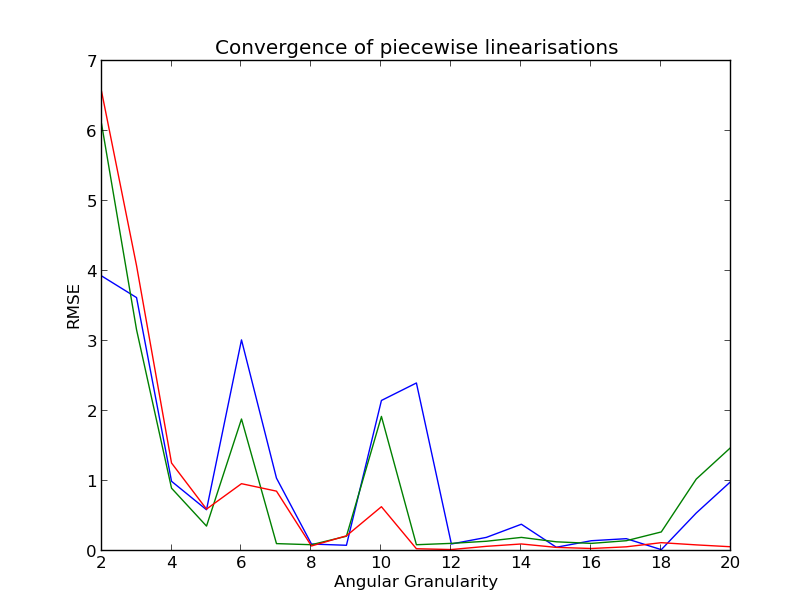
Figure 2: The RMSE of voltages on Garver6y for piece-wise linearisations as a function of the number of segments used in the piece-wise linearisation of the voltage angle per each 90 degrees.

Finally, the performance of the lift-and-branch-and-bound procedure is somewhat promising. Even a simple, preliminary implementation traverses a tree of 15 subproblems in 59873 seconds using SeDuMi, the SDP solver. We envision this could be sped up much further.

VII Conclusions

Whereas in the operations of power systems, piece-wise linearisations may soon be replaced by convex relaxations [21, 20, 1], the outlook remains less clear within investment planning. Although polynomial optimisation allows for global optimisation in power systems with accurate models for the physics, it remains a challenge to develop solvers that would scale to realistic instances, especially considering multiple scenarios. Considering also that the Lavaei-Low relaxation seems difficult to extend to the investment decisions, one can hardly enumerate all the possible configurations and test them with an interior-point method, and the scalability of the piece-wise linearisations is also limited, it seems worth studying the polynomial optimisation approach in more detail.

The first results obtained with the lift-and-branch-and-bound method give some indication on how to make approaches based on polynomial optimisation applicable to investment planning in power systems, which involves both, discrete decisions and accurate models of the non-convex power flow in the constraints. If this approach proves to be scalable for larger instances, it may potentially be applied to investment planning problems beyond power systems, where there is a combined challenge of discrete investment decisions, continuous operational decisions and non-convex system dynamics, such as in gas and water network optimisation or in traffic management. We conjecture that the lift-and-branch-and-bound method has finite convergence for a large class of instances, although we do not prove so in this paper, and envision much further research focussed on it.

References

- [1] B. Ghaddar, J. Marecek, and M. Mevissen, “Optimal power flow as a polynomial optimization problem,” Power Systems, IEEE Transactions on, vol. to appear, 2015.
- [2] H. Zhang, G. Heydt, V. Vittal, and J. Quintero, “An improved network model for transmission expansion planning considering reactive power and network losses,” Power Systems, IEEE Transactions on, vol. 28, pp. 3471–3479, Aug 2013.
- [3] N. Alguacil, A. Motto, and A. Conejo, “Transmission expansion planning: a mixed-integer lp approach,” Power Systems, IEEE Transactions on, vol. 18, pp. 1070–1077, Aug 2003.
- [4] E. B. Fisher, R. P. O’Neill, and M. C. Ferris, “Optimal transmission switching,” IEEE Transactions on Power Systems, 2008.
- [5] R. P. O Neill, A. Castillo, and M. B. Cain, “The iv formulation and linear approximations of the ac optimal power flow problem — optimal power flow paper 2,” December 2012.
- [6] R. Ferreira, C. Borges, and M. Pereira, “Distribution network reconfiguration under modeling of ac optimal power flow equations: A mixed-integer programming approach,” in Innovative Smart Grid Technologies Latin America (ISGT LA), 2013 IEEE PES Conference On, pp. 1–8, IEEE, 2013.
- [7] P. Trodden, W. Bukhsh, A. Grothey, and K. McKinnon, “Optimization-based islanding of power networks using piecewise linear ac power flow,” Power Systems, IEEE Transactions on, vol. 29, pp. 1212–1220, May 2014.
- [8] M. F. Anjos and J.-B. Lasserre, eds., Handbook on semidefinite, conic and polynomial optimization, vol. 166 of International series in operations research & management science. New York: Springer, 2012.
- [9] M. Choi, T. Lam, and B. Reznick, “Sums of squares of real polynomials,” in Proc. of Symposia in Pure Mathematics, 1995.
- [10] J. Lasserre, “Global optimization problems with polynomials and the problem of moments,” SIAM Journal on Optimization, vol. 11, pp. 796–817, 2001.
- [11] J. Lasserre, “Convergent SDP-relaxations in polynomial optimization with sparsity,” SIAM Journal on Optimization, vol. 17, no. 3, pp. 882–843, 2006.
- [12] H. Waki, S. Kim, M. Kojima, and M. Muramatsu, “Sums of squares and semidefinite programming relaxations for polynomial optimization problems with structured sparsity,” SIAM Journal on Optimization, vol. 17, no. 1, pp. 218–242, 2006.
- [13] M. Kojima and M. Muramatsu, “A note on sparse SOS and SDP relaxations for polynomial optimization problems over symmetric cones,” Computational Optimization and Applications, vol. 42, no. 1, pp. 31–41, 2009.
- [14] O. Günlük and J. Linderoth, “Perspective reformulations of mixed integer nonlinear programs with indicator variables,” Mathematical programming, vol. 124, no. 1-2, pp. 183–205, 2010.
- [15] A. H. Land and A. G. Doig, “An automatic method of solving discrete programming problems,” Econometrica, pp. 497–520, 1960.
- [16] R. E. Curto and L. A. Fialkow, Flat Extensions of Positive Moment Matrices: Recursively Generated Relations: Recursively Generated Relations, vol. 648. American Mathematical Society, 1998.
- [17] W. A. Bukhsh, A. Grothey, K. I. McKinnon, and P. Trodden, “Local solutions of optimal power flow,” Power Systems, IEEE Transactions on, vol. 28, no. 4, pp. 4780–4788, 2013.
- [18] L. L. Garver, “Transmission network estimation using linear programming,” Power Apparatus and Systems, IEEE Transactions on, no. 7, pp. 1688–1697, 1970.
- [19] R. D. Zimmerman, C. E. Murillo-Sánchez, and R. J. Thomas, “Matpower: Steady-state operations, planning and analysis tools for power systems research and education,” Power Systems, IEEE Transactions on, vol. 26, no. 1, pp. 12–19, 2011.
- [20] D. Molzahn, J. Holzer, B. Lesieutre, and C. DeMarco, “Implementation of a large-scale optimal power flow solver based on semidefinite programming,” IEEE Transactions on Power Systems, vol. 28, no. 4, pp. 3987–3998, 2013.
- [21] J. Lavaei and S. Low, “Zero duality gap in optimal power flow problem,” Power Systems, IEEE Transactions on, vol. 27, no. 1, pp. 92–107, 2012.