Signal of right-handed currents using ${B\to{K^{\!*}}\ell^{+}\ell^{-}}$ observables at the kinematic endpoint.

Abstract

The decay mode $B\to{K^{\!*}}\ell^{+}\ell^{-}$ is one of the most promising modes to probe physics beyond the standard model (SM), since the angular distribution of the decay products enable measurement of several constraining observables. LHCb has recently measured these observables using $3\mbox{\,fb}^{-1}$ of data as a binned function of $q^{2}$, the dilepton invariant mass squared. We find that LHCb data implies evidence for right-handed currents, which are absent in the SM. These conclusions are derived in the maximum $q^{2}$ limit and are free from hadronic corrections. Our approach differs from other approaches that probe new physics at low $q^{2}$ as it does not require estimates of hadronic parameters but relies instead on heavy quark symmetries that are reliable at the maximum $q^{2}$ kinematic endpoint.

I Introduction

The rare decay $B\to{K^{\!*}}\ell^{+}\ell^{-}$, which involves a $b\rightarrow s$ flavor changing loop induced quark transition at the quark level, provides an indirect but very sensitive probe of new physics (NP) beyond the standard model (SM). The angular distribution of the decay products provides a large number of observables  [1] and thus can be used to reduce hadronic uncertainties making the mode a very special tool to probe for NP. Significant work has been done to probe NP in this mode. Most previous attempts have focused [2] on the low dilepton invariant mass squared region $q^{2}=1-6~{}\mathrm{\,Ge\kern-1.00006ptV}^{2}$. An alternative approach that probes the maximum $q^{2}$ limit has also been studied in literature [3, 4]. We show that this limit holds significant promise for clean probes of NP. A previous study suggested a possible signal of NP in the large $q^{2}$ region [5]. In this letter we show that LHCb data implies a $5\sigma$ signal for the existence of NP. While the evidence for right handed currents is clear, other NP contributions are also possible. Our conclusions are derived in the maximum $q^{2}$ limit ($q^{2}_{\scriptscriptstyle\text{max}}$) and are free from hadronic corrections. Our approach differs from other approaches that probe NP at low $q^{2}$ by not requiring estimates of hadronic parameters but relying instead on heavy quark symmetries that are completely reliable at the kinematic endpoint $q^{2}_{\scriptscriptstyle\text{max}}$ [3, 6]. While the observables themselves remain unaltered from their SM values, their derivatives and second derivatives at the endpoint are sensitive to NP effects. The paper is organized as follows. In Sec. II, we discuss the model independent theoretical framework used for the analysis. The numerical procedure for the extraction of right-handed (RH) currents is described in Sec. III. We illustrate the effect of resonances and the convergence of the polynomial fit in Sec. IV and Sec. V, respectively. Finally, Sec. VI contains concluding remarks.

II Theoretical Formalism

In this section we briefly discuss the model independent theoretical framework that has been adopted in this work. The decay $B\to{K^{\!*}}\ell^{+}\ell^{-}$ is described by six transversity amplitudes that can be written as [7]

$$\mathcal{A}_{\lambda}^{L,R}=C_{L,R}^{\scriptscriptstyle\lambda}\,\mathcal{F}_{\lambda}-\widetilde{\mathcal{G}}_{\lambda}=\big{(}\widetilde{C}_{9}^{\scriptscriptstyle\lambda}\mp C_{10})\mathcal{F}_{\lambda}-\widetilde{\mathcal{G}}_{\lambda}$$ (1)

within the standard model in the massless lepton limit [8]. This parametric form of the amplitude is general enough to comprehensively include all short-distance and long-distance effects, factorizable and nonfactorizable contributions, resonance contributions and complete electromagnetic corrections to hadronic operators up to all orders. In Eq. (1) $C_{9}$ and $C_{10}$ are Wilson coefficients with $\widetilde{C}_{9}^{\scriptscriptstyle\lambda}$ being the redefined “effective” Wilson coefficient defined [7, 10, 9] as

$$\widetilde{C}_{9}^{\scriptscriptstyle\lambda}=C_{9}+\Delta C_{9}^{\text{(fac)}}(q^{2})+\Delta C_{9}^{{\scriptscriptstyle\lambda}{\text{,(non-fac)}}}(q^{2})$$ (2)

where $\Delta C_{9}^{\text{(fac)}}(q^{2})$, $\Delta C_{9}^{{\scriptscriptstyle\lambda}{\text{,(non-fac)}}}(q^{2})$ correspond to factorizable and soft gluon non-factorizable contributions. The Wilson coefficient $C_{10}$ is unaffected by strong interaction effects coming from electromagnetic corrections to hadronic operators [11]. The form factors $\mathcal{F}_{\lambda}$ and $\widetilde{\mathcal{G}}_{\lambda}$ introduced in Eq. (1) can in principle be related to the conventional form factors describing the decay if power corrections are ignored. However, our approach does not rely on estimates of $\mathcal{F}_{\lambda}$ and $\widetilde{\mathcal{G}}_{\lambda}$.

In the SM, $\mathcal{F}_{\lambda}$’s and $C_{10}$ are real, whereas $\widetilde{C}_{9}^{\scriptscriptstyle\lambda}$ and $\widetilde{\mathcal{G}}_{\lambda}$ contain the imaginary contributions of the amplitudes. Defining two variables $r_{\lambda}$ and $\varepsilon_{\lambda}$, the amplitudes ${\cal A}_{\lambda}^{L,R}$ in Eq. (1) can be rewritten as,

$$\mathcal{A}_{\lambda}^{L,R}=(\mp C_{10}-r_{\lambda})\mathcal{F}_{\lambda}+i\varepsilon_{\lambda},$$ (3)

where

$$r_{\lambda} = \frac{\text{Re}(\widetilde{\mathcal{G}}_{\lambda})}{\mathcal{F}_{\lambda}}-\text{Re}(\widetilde{C}_{9}^{\scriptscriptstyle{\lambda}}),$$ (4)

$$\varepsilon_{\lambda} = \text{Im}(\widetilde{C}_{9}^{\scriptscriptstyle{\lambda}})\mathcal{F}_{\lambda}-\text{Im}(\widetilde{\mathcal{G}}_{\lambda}).$$ (5)

The observables $F_{\perp}$, $F_{\|}$, $F_{L}$, $A_{\text{FB}}$ and $A_{5}$ are defined as,

$$F_{\lambda} =\frac{|\mathcal{A}_{\lambda}^{L}|^{2}+|\mathcal{A}_{\lambda}^{R}|^{2}}{\displaystyle\Gamma_{\!f}}~{}~{}~{}\lambda\in\{\perp,\|,0\},$$ (6)

$$A_{\text{FB}} =\frac{3}{2}\frac{\text{Re}({\cal A}_{\|}^{L}{\cal A}_{\perp}^{L^{*}}-{\cal A}_{\|}^{R}{\cal A}_{\perp}^{R^{*}})}{\Gamma_{\!f}},$$ (7)

$$A_{5} =\frac{3}{2\sqrt{2}}\frac{\text{Re}(\mathcal{A}_{0}^{L}\mathcal{A}_{\perp}^{L^{*}}-\mathcal{A}_{0}^{R}\mathcal{A}_{\perp}^{R^{*}})}{\Gamma_{\!f}},$$ (8)

where $\Gamma_{\!\!f}\equiv\sum_{\lambda}(|{\cal A}_{\lambda}^{L}|^{2}+|{\cal A}_{\lambda}^{R}|^{2})$ and are related to the observables measured by LHCb [14] as follows:

$$F_{\perp} =\frac{1-F_{L}+2S_{3}}{2},~{}~{}A_{4}=-\displaystyle\frac{2}{\pi}S_{4},$$

$$~{}~{}A_{5} =\displaystyle\frac{3}{4}S_{5},~{}~{}~{}A_{\text{FB}}\!=\!-A_{\text{FB}}^{\scriptscriptstyle\text{LHCb}}.$$ (9)

We neglect the $\varepsilon_{\lambda}$ contributions to the amplitude for the time being, but their effect in the numerical analysis is discussed in Appendix A. In the presence of RH currents the transversity amplitudes are given by [11]

$$\mathcal{A}^{L,R}_{\perp} =\big{(}(\widetilde{C}_{9}^{\scriptscriptstyle{\perp}}+C_{9}^{\prime})\mp(C_{10}+C_{10}^{\prime})\big{)}\mathcal{F}_{\perp}-\widetilde{\mathcal{G}}_{\perp}$$ (10)

$$\mathcal{A}^{L,R}_{\|} =\big{(}(\widetilde{C}_{9}^{\scriptscriptstyle{\|}}-C_{9}^{\prime})\mp(C_{10}-C_{10}^{\prime})\big{)}\mathcal{F}_{\|}-\widetilde{\mathcal{G}}_{\|}$$ (11)

$$\mathcal{A}^{L,R}_{0} =\big{(}(\widetilde{C}_{9}^{\scriptscriptstyle{0}}-C_{9}^{\prime})\mp(C_{10}-C_{10}^{\prime})\big{)}\mathcal{F}_{0}-\widetilde{\mathcal{G}}_{0}.$$ (12)

Note that setting the RH contributions $C_{9}^{\prime}$ and $C_{10}^{\prime}$ to zero, the amplitudes reduce to the SM ones in Eq. (1).

Introducing new variables

$$\xi=\frac{C_{10}^{\prime}}{C_{10}}~{}~{}\text{and}~{}~{}\xi^{\prime}=\frac{C_{9}^{\prime}}{C_{10}}$$ (13)

the observables $F_{\!\perp}$, $F_{\|}$, $A_{\text{FB}}$, $A_{5}$ (Eqs. (6) – (8)) can be expressed as,

$$F_{\!\perp} =2\zeta\,(1+\xi)^{2}(1+R_{\perp}^{2})$$ (14)

$$F_{\|}\mathsf{P_{1}^{2}} =2\zeta\,(1-\xi)^{2}(1+R_{\|}^{2})$$ (15)

$$F_{L}\mathsf{P_{2}^{2}} =2\zeta\,(1-\xi)^{2}(1+R_{0}^{2})$$ (16)

$$A_{\text{FB}}\mathsf{P_{1}} =3\zeta\,(1-\xi^{2})\big{(}R_{\|}+R_{\perp}\big{)}$$ (17)

$$\sqrt{2}A_{5}\mathsf{P_{2}} =3\zeta\,(1-\xi^{2})\big{(}R_{0}+R_{\perp}\big{)}$$ (18)

where $\mathsf{P_{1}}=\displaystyle\frac{\mathcal{F}_{\perp}}{\mathcal{F}_{\|}}$,   $\mathsf{P_{2}}=\displaystyle\frac{\mathcal{F}_{\perp}}{\mathcal{F}_{0}},~{}~{}\zeta=\frac{\mathcal{F}_{\perp}^{2}C_{10}^{2}}{\Gamma_{\!\!f}}$,

$$R_{\perp}=\frac{\displaystyle\frac{r_{\perp}}{C_{10}}-\xi^{\prime}}{1+\xi},~{}R_{\|}=\frac{\displaystyle\frac{r_{\|}}{C_{10}}+\xi^{\prime}}{1-\xi},~{}R_{0}=\frac{\displaystyle\frac{r_{0}}{C_{10}}+\xi^{\prime}}{1-\xi}.$$ (19)

We consider the observables $F_{L}$, $F_{\|}$, $F_{\perp}$, $A_{\text{FB}}$ and $A_{5}$, with the constraint $F_{L}+F_{\|}+F_{\perp}=1$. Using Eq. (14)–(18), we obtain expressions for $R_{\perp}$, $R_{\|}$, $R_{0}$ and $\mathsf{P}_{2}$ in terms of the observables and $\mathsf{P}_{1}$:

$$R_{\perp} =\pm\frac{3}{2}\frac{\Big{(}\frac{1-\xi}{1+\xi}\Big{)}F_{\perp}+\frac{1}{2}\mathsf{P_{1}}Z_{1}}{\mathsf{P_{1}}A_{\text{FB}}}$$ (20)

$$R_{\|} =\pm\frac{3}{2}\frac{\Big{(}\frac{1+\xi}{1-\xi}\Big{)}\mathsf{P_{1}}F_{\|}+\frac{1}{2}Z_{1}}{A_{\text{FB}}}$$ (21)

$$R_{0} =\pm\frac{3}{2\sqrt{2}}\frac{\Big{(}\frac{1+\xi}{1-\xi}\Big{)}\mathsf{P_{2}}F_{L}+\frac{1}{2}Z_{2}}{A_{5}}$$ (22)

$$\mathsf{P_{2}} =\!\frac{\Big{(}\frac{1-\xi}{1+\xi}\Big{)}2\mathsf{P_{1}}A_{\text{FB}}F_{\perp}}{\sqrt{2}A_{5}\left(\Big{(}\frac{1-\xi}{1+\xi}\Big{)}2F_{\perp}+Z_{1}\mathsf{P_{1}}\right)-Z_{2}\mathsf{P_{1}}A_{\text{FB}}}$$ (23)

where $Z_{1}=(4F_{\|}F_{\perp}-\frac{16}{9}A_{\text{FB}}^{2})^{\nicefrac{{1}}{{2}}}$ and $Z_{2}=(4F_{L}F_{\perp}-\frac{32}{9}A_{5}^{2})^{\nicefrac{{1}}{{2}}}$. Since we have one extra parameter compared to observables, all of the above expressions depend on $\mathsf{P_{1}}$. Fortunately in the large $q^{2}$ limit, the relations between form factors enable us to eliminate one parameter.

At the kinematic limit $q^{2}=q^{2}_{\scriptscriptstyle\text{max}}=(m_{B}-m_{K^{\!*}})^{2}$ the ${K^{\!*}}$ meson is at rest and the two leptons travel back to back in the $B$ meson rest frame. There is no preferred direction in the decay kinematics. Hence, the differential decay distribution in this kinematic limit must be independent of the angles $\theta_{\ell}$ and $\phi$, which can be integrated out. This imposes constraints on the amplitude $A_{\lambda}^{L,R}$ and hence the observables. The entire decay, including the decay ${K^{\!*}}\to K\pi$ takes place in a single plane, resulting in a vanishing contribution to the ‘$\perp$’ helicity, or $F_{\perp}=0$. Since the ${K^{\!*}}$ decays at rest, the distribution of $K\pi$ is isotropic and cannot depend on $\theta_{K}$. It can easily be seen that this is only possible if $F_{\|}=2F_{L}$ [6].

At $q^{2}\!=\!q^{2}_{\scriptscriptstyle\text{max}}$, $\Gamma_{\!\!f}\to 0$ as all the transversity amplitudes vanish in this limit. The constraints on the amplitudes described above result in unique values of the helicity fractions and the asymmetries at this kinematical endpoint. The values of the helicity fractions and asymmetries were derived in Ref. [6, 7] where it is explicitly shown that

$$\displaystyle F_{L}(q^{2}_{\scriptscriptstyle\text{max}})=\frac{1}{3}, F_{\|}(q^{2}_{\scriptscriptstyle\text{max}})=\displaystyle\frac{2}{3}, A_{4}(q^{2}_{\scriptscriptstyle\text{max}})=\displaystyle\frac{2}{3\pi},~{}~{}~{}~{}~{}~{}$$

$$F_{\perp}(q^{2}_{\scriptscriptstyle\text{max}})=0,~{} A_{\text{FB}}(q^{2}_{\scriptscriptstyle\text{max}})=0,~{} A_{5,7,8,9}(q^{2}_{\scriptscriptstyle\text{max}})=0.$$ (24)

The large $q^{2}$ region where the ${K^{\!*}}$ has low-recoil energy has also been studied [3, 12] in a modified heavy quark effective theory framework. In the limit $q^{2}\to q^{2}_{\scriptscriptstyle\text{max}}$ the hadronic form factors satisfy the conditions

$$\frac{\widetilde{\mathcal{G}}_{\|}}{\mathcal{F}_{\|}}=\frac{\widetilde{\mathcal{G}}_{\perp}}{\mathcal{F}_{\perp}}=\frac{\widetilde{\mathcal{G}}_{0}}{\mathcal{F}_{0}}=-\kappa\frac{2m_{b}m_{B}C_{7}}{q^{2}},$$ (25)

where $\kappa\approx 1$ as shown in [12]. The helicity independence of the ratios ${\widetilde{\mathcal{G}}_{\lambda}}/{\mathcal{F}_{\lambda}}$ at $q^{2}_{\scriptscriptstyle\text{max}}$ is easy to understand, since both the $B$ and ${K^{\!*}}$ mesons are at rest, resulting in a complete overlap of the wave functions of these two mesons and the absence of any preferred direction in the $K\pi$ distribution. Due to the constraints arising from decay kinematics and Lorentz invariance, on the observables at $q^{2}_{\scriptscriptstyle\text{max}}$ (in Eq. (II)), it is shown in Ref. [6] that the non-factorizable contributions are helicity independent at the endpoint. Hence from Eq. (4) it can be seen that, $r_{0}=r_{\|}=r_{\perp}\equiv r$ [13]. Therefore, Eq. (19) implies that, by definition of the variables $R_{\lambda}$, in the presence of RH currents, one should expect $R_{0}=R_{\parallel}\neq R_{\perp}$ at $q^{2}=q^{2}_{\scriptscriptstyle\text{max}}$ without any approximation. As argued above this relation is unaltered by non-factorizable and resonance contributions at this kinematic endpoint.

We study the values of $R_{\lambda}$, $\zeta$ and $P_{1,2}$ in the large $q^{2}$ region and consider the kinematic limit $q^{2}\to q^{2}_{\scriptscriptstyle\text{max}}$. It is easy to see from Eq. (14) that $F_{\perp}(q^{2}_{\scriptscriptstyle\text{max}})=0$ implies that $\zeta=0$ in the limit $q^{2}\to q^{2}_{\scriptscriptstyle\text{max}}$. Further, since $R_{\parallel}(q^{2}_{\scriptscriptstyle\text{max}})=R_{0}(q^{2}_{\scriptscriptstyle\text{max}})$, Eqs. (15) and (16) imply that in the limit $q^{2}\to q^{2}_{\scriptscriptstyle\text{max}}$, $\mathsf{P}_{2}=\sqrt{2}\,\mathsf{P}_{1}$. However, both $\mathsf{P}_{1}$ and $\mathsf{P}_{2}$ go to zero at $q^{2}_{\scriptscriptstyle\text{max}}$. It is therefore imperative that we take into account the limiting values very carefully by Taylor expanding all observables around the endpoint $q^{2}_{\scriptscriptstyle\text{max}}$ in terms of the variable $\delta\equiv q^{2}_{\scriptscriptstyle\text{max}}-q^{2}$. The leading power of $\delta$ in the Taylor expansion must take into account the relative momentum dependence of the amplitudes ${\cal A}_{\lambda}^{L,R}$. Eq. (6)-(8) and (II) together imply that $\mathcal{A}_{\perp}^{L,R}$ must have an expansion at least $\mathcal{O}(\sqrt{\delta})$ higher compared to $\mathcal{A}_{\|,0}^{L,R}$. This is in agreement with Ref. [6]. Hence the leading term in $F_{L}$ and $F_{\|}$ must be ${\cal O}(\delta^{0})$, whereas the leading term for $F_{\perp}$ is ${\cal O}(\delta)$. The leading terms for the asymmetries, $A_{5}$ and $A_{\text{FB}}$, are ${\cal O}(\sqrt{\delta})$. Thus, we expand the observables as follows:

$$F_{L} =\frac{1}{3}+F_{L}^{(1)}\delta+F_{L}^{(2)}\delta^{2}+F_{L}^{(3)}\delta^{3}$$ (26)

$$F_{\perp} =F_{\perp}^{(1)}\delta+F_{\perp}^{(2)}\delta^{2}+F_{\perp}^{(3)}\delta^{3}$$ (27)

$$A_{\text{FB}} =A_{\text{FB}}^{(1)}\delta^{\nicefrac{{1}}{{2}}}+A_{\text{FB}}^{(2)}\delta^{\nicefrac{{3}}{{2}}}+A_{\text{FB}}^{(3)}\delta^{\nicefrac{{5}}{{2}}}$$ (28)

$$A_{5} =A_{5}^{(1)}\delta^{\nicefrac{{1}}{{2}}}+A_{5}^{(2)}\delta^{\nicefrac{{3}}{{2}}}+A_{5}^{(3)}\delta^{\nicefrac{{5}}{{2}}},$$ (29)

where for each observable $O$, $O^{(n)}$ is the coefficient of the $n^{\text{th}}$ term in the expansion. The polynomial fit to data is not based on Heavy Quark Effective Theory (HQET) or any other theoretical assumption. A parametric fit to data is performed, so as to obtain the limiting values of the coefficients to determine the slope and second derivative of the observables at $q^{2}_{\scriptscriptstyle\text{max}}$. It should be noted that the polynomial parameterizations are inadequate to describe the $q^{2}$ dependent behavior of resonances. However, systematics of resonance effects are discussed in Sec. IV in detail validating the approach followed here.

The relation in Eq. (25) between form factors is expected to be satisfied in the large $q^{2}$ region. Eq. (25) is naturally satisfied if it is valid at each order in the Taylor expansion of the form factors:

$$q^{2}\frac{\widetilde{\mathcal{G}}_{\lambda}}{\mathcal{F}_{\lambda}}=q^{2}_{\scriptscriptstyle\text{max}}\frac{\widetilde{\mathcal{G}}_{\lambda}^{(1)}+\displaystyle\delta\,(\widetilde{\mathcal{G}}_{\lambda}^{(2)}-\displaystyle\frac{\widetilde{\mathcal{G}}_{\lambda}^{(1)}}{q^{2}_{\scriptscriptstyle\text{max}}})+{\cal O}(\delta^{2})}{\mathcal{F}_{\lambda}^{(1)}+\delta\,\mathcal{F}_{\lambda}^{(2)}+{\cal O}(\delta^{2})}.$$ (30)

We require only that the relation be valid up to order $\delta$. In order for Eq. (30) to have a constant value in the neighborhood of $q^{2}_{\scriptscriptstyle\text{max}}$ up to ${\cal O}(\delta)$, we must have $\mathcal{F}_{\lambda}^{(2)}=c\,\mathcal{F}_{\lambda}^{(1)}$ and $(q^{2}_{\scriptscriptstyle\text{max}}\,\widetilde{\mathcal{G}}_{\lambda}^{(2)}-\widetilde{\mathcal{G}}_{\lambda}^{(1)})=c\,q^{2}_{\scriptscriptstyle\text{max}}\,\widetilde{\mathcal{G}}_{\lambda}^{(1)}$ where $c$ is any constant. As discussed earlier, $\mathsf{P_{2}}=\sqrt{2}\mathsf{P_{1}}$ at $q^{2}_{\scriptscriptstyle\text{max}}$, hence, we must have $\mathsf{P_{2}^{(1)}}=\sqrt{2}\mathsf{P_{1}^{(1)}}$, where $\mathsf{P_{1,2}^{(1)}}$ are the coefficients of the leading ${\cal O}(\sqrt{\delta})$ term in the expansion. However, the above argument implies that at the next order, we must also have $\mathsf{P_{2}^{(2)}}=\sqrt{2}\mathsf{P_{1}^{(2)}}$, since $\mathcal{F}_{\lambda}^{(2)}=c\,\mathcal{F}_{\lambda}^{(1)}$. This provides the needed input that together with Eq. (23) determines $\mathsf{P_{1}^{(1)}}$ purely in terms of observables.

The expressions for $R_{\lambda}$ in the limit $q^{2}\to q^{2}_{\scriptscriptstyle\text{max}}$ are

$$R_{\perp}(q^{2}_{\scriptscriptstyle\text{max}}) =\!\displaystyle\frac{8A_{\text{FB}}^{(1)}(-2A_{5}^{(2)}+A_{\text{FB}}^{(2)})+9(3F_{L}^{(1)}+F_{\perp}^{(1)})F_{\perp}^{(1)}}{8\,(2A_{5}^{(2)}-A_{\text{FB}}^{(2)})\,\sqrt{\frac{3}{2}F_{\perp}^{(1)}-A_{\text{FB}}^{(1)\,2}}}$$

$$=\displaystyle\frac{\omega_{2}-\omega_{1}}{\omega_{2}\sqrt{\omega_{1}-1}},$$ (31)

$$R_{\|}(q^{2}_{\scriptscriptstyle\text{max}}) =\displaystyle\frac{3(3F_{L}^{(1)}+F_{\perp}^{(1)})\,\sqrt{\frac{3}{2}F_{\perp}^{(1)}-A_{\text{FB}}^{(1)\,2}}}{\displaystyle-8A_{5}^{(2)}+4A_{\text{FB}}^{(1)}+3A_{\text{FB}}^{(1)}(3F_{L}^{(1)}+F_{\perp}^{(1)})}$$

$$=\displaystyle\frac{\sqrt{\omega_{1}-1}}{\omega_{2}-1}=R_{0}(q^{2}_{\scriptscriptstyle\text{max}})$$ (32)

where

$$\omega_{1}= \displaystyle\frac{3}{2}\frac{F_{\perp}^{(1)}}{A_{\text{FB}}^{(1)\,2}}\text{~{}~{}and~{}~{}}\omega_{2}= \displaystyle\frac{4\,(2A_{5}^{(2)}-A_{\text{FB}}^{(2)})}{3\,A_{\text{FB}}^{(1)}(3F_{L}^{(1)}+F_{\perp}^{(1)})}.$$ (33)

It should be noted that Eqs. (31)–(33) are derived only at $q^{2}_{\scriptscriptstyle\text{max}}$. However, even at the endpoint, the expressions depend on polynomial coefficients: $F_{L}^{(1)}$ and $F_{\perp}^{(1)}$ as well as $A_{\text{FB}}^{(2)}$ and $A_{5}^{(2)}$ which are not related by HQET. Hence, in our approach, corrections beyond HQET are automatically incorporated through fits to data.

In the absence of RH currents or other NP that treats the “$\perp$” amplitude differently one would expect $R_{\perp}(q^{2}_{\scriptscriptstyle\text{max}})=R_{\|}(q^{2}_{\scriptscriptstyle\text{max}})=R_{0}(q^{2}_{\scriptscriptstyle\text{max}})$. It is easily seen that the LHS of Eq. (17) is positive around $q^{2}_{\scriptscriptstyle\text{max}}$ and since $\zeta>0$, we must have $R_{\perp}=R_{\|}=R_{0}>0$. Since very large contributions from RH currents are not possible, as they would have been seen elsewhere, $R_{\lambda}(q^{2}_{\scriptscriptstyle\text{max}})>0$ still holds and restricts $\xi$ and $\xi^{\prime}$ to reasonably small values.

	$O^{(1)}(10^{-2})$	$O^{(2)}(10^{-3})$	$O^{(3)}(10^{-4})$
$F_{L}$	$-2.85\pm 1.26$	$~{}12.13\pm 1.90$	$-5.68\pm 0.67$
$F_{\perp}$	$~{}6.89\pm 1.65$	$-9.79\pm 2.47$	$~{}3.83\pm 0.86$
$A_{\text{FB}}$	$-30.58\pm 1.95$	$~{}26.96\pm 3.58$	$-4.15\pm 1.47$
$A_{5}$	$-15.85\pm 1.87$	$~{}5.38\pm 3.33$	$2.46\pm 1.29$

Table 1: Best fit and 1$\sigma$ uncertainties for the coefficients of observables (in Eqs. (26)– (29)) obtained by fitting recent LHCb’s 14- bin measurements [14] as a function of $q^{2}$ for the entire region.

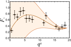
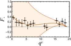
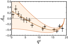
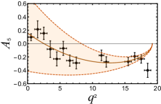
Figure 1: An analytic fit to 14-bin LHCb data using Taylor expansion at $q^{2}_{\scriptscriptstyle\text{max}}$ for the observables $F_{L}$, $F_{\perp}$, $A_{\text{FB}}$ and $A_{5}$ are shown as the brown curves. The $\pm 1\sigma$ error bands are indicated by the light brown shaded regions, derived including correlation among all observables. The points with the black error bars are LHCb 14-bin measurements [14].

III Right-Handed current Analysis

In this section we describe the numerical analysis based on the theoretical formalism derived in the previous section. We start by fitting the latest LHCb measurements [14] of the observables $F_{L}$, $F_{\perp}$, $A_{\text{FB}}$ and $A_{5}$ as functions of $q^{2}$ using the Taylor expansion at $q^{2}_{\scriptscriptstyle\text{max}}$ as given in Eqs. (26)– (29). The fits were performed by minimizing the $\chi^{2}$ function, which compares the bin integrated values of $q^{2}$ functions of the observables with their measured experimental values for all 14 bins. The correlations reported by LHCb among all observables have also been considered. The bin integration for the polynomial fit is weighted with the recent measurements of differential decay rate [15]. A polynomial is fitted for $d\Gamma/dq^{2}$ data for the entire $q^{2}$ region. This fitted polynomial for $d\Gamma/dq^{2}$ (say denoted by $\Gamma(q^{2})$) is then used in weighted average for all the observables. For an observable $\mathcal{O}$ the bin averaged value within the $q^{2}$ interval $[b_{i},b_{f}]$ is obtained by, $\int_{b_{i}}^{b_{f}}\mathcal{O}(q^{2})\Gamma(q^{2})\,dq^{2}\Big{/}\int_{b_{i}}^{b_{f}}\Gamma(q^{2})\,dq^{2}$. We use the 14 bin data set based on the method of moments [16] from LHCb rather than the 8 bin data set as it enables better constraints near $q^{2}_{\scriptscriptstyle\text{max}}$. The best fit values for each coefficient of the observables $F_{L}$, $F_{\perp}$, $A_{\text{FB}}$ and $A_{5}$ (Eqs. (26)– (29)) are given in Table 1. The errors in each coefficient are evaluated using a covariance matrix technique. A detailed study of the systematics in fitting the polynomial is described in Sec. V. Variations in the order of the polynomial from two to four and the number of bins used in fitting (from the last four to all fourteen), demonstrate good convergence when larger numbers of bins are considered.

In Fig. 1 the results of the fits for the observables $F_{L}$, $F_{\perp}$, $A_{\text{FB}}$ and $A_{5}$, respectively, are compared with the measured LHCb data [14]. We notice that the factorization requirement $A_{\text{FB}}^{(1)}=2A_{5}^{(1)}$ holds to within $\pm 1\sigma$. We treat $A_{\text{FB}}^{(1)}$ and $2A_{5}^{(1)}$ as two independent measurements of the same quantity as we have neglected correlation between observables. We obtain $\omega_{1}=1.10\pm 0.30~{}(1.03\pm 0.34)$ and $\omega_{2}=-4.19\pm 10.48~{}(-4.04\pm 10.12)$, where the first values are determined using $A_{\text{FB}}^{(1)}$ and the values in the round brackets use $2A_{5}^{(1)}$.

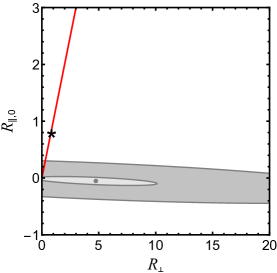
Figure 2: Allowed regions in $R_{\perp}$ – $R_{\|,0}$ plane are shown. The solid red straight line on the far left corresponds to the case $R_{\perp}=R_{\|,0}$. The SM value is indicated by the star. The gray point corresponds to best fit central values. The light and dark gray contours correspond to $1\sigma$ and $5\sigma$ confidence level regions, respectively.

We estimate the range of values for $R_{\perp}$ and $R_{\|,0}$ in two different ways. One approach estimates $R_{\perp}$ and $R_{\|,0}$ using randomly chosen values of $F_{L}^{(1)}$, $F_{P}^{(1)}$, $A_{\text{FB}}^{(1)}$, $A_{5}^{(1)}$, $A_{\text{FB}}^{(2)}$ and $A_{5}^{(2)}$, from a Gaussian distribution with the central value as the mean and errors from Table 1. If RH currents are absent the values would lie along a straight line with a $45^{\text{o}}$ slope in the $R_{\perp}-R_{\|,0}$ plane. However, we find a slope that is nearly horizontal, indicating that $R_{\perp}\gg R_{\|,0}$. The deviation of slope from $45^{\text{o}}$ provides evidence of contributions from RH currents.

In an alternate approach we fit the values of $R_{\perp}$ and $R_{\|,0}$ with the two estimated values of $\omega_{1}$ and $\omega_{2}$ by minimizing a $\chi^{2}$ function. The allowed regions in the $R_{\perp}$ – $R_{\|,0}$ plane are shown in Fig. 2. The solid red straight line on the far left corresponds to the case $R_{\perp}=R_{\|,0}$. The SM value is indicated by the star on the red line. The light gray and dark gray contours indicate the $1\sigma$ and $5\sigma$ permitted regions. We emphasize that for the SM, even in the presence of resonances the contours should be aligned along the $45^{\text{o}}$ line, since resonances contribute equally to all helicities through $\Delta C_{9}$ in Eq. (2). Hence the deviation of the contours from the SM expectation is a signal for RH currents. As it will be discussed in Sec. IV, charmonium resonance contributions in bin averaged data always raise the values of $\omega_{1}$, whereas we find that the values of $\omega_{1}$ are close to the lowest possible physical value allowed.

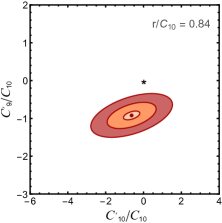
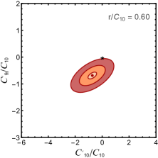
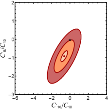
Figure 3: Allowed regions in $C_{10}^{\prime}/C_{10}$ – $C_{9}^{\prime}/C_{10}$ plane are shown in three different panels. The yellow, orange and red bands are the 1$\sigma$, 3$\sigma$ and 5$\sigma$ confidence level regions, respectively. The center red dot denotes best fit point; the SM values of $C_{10}^{\prime}/C_{10}$ and $C_{9}^{\prime}/C_{10}$ are indicated by a ‘star’, which sits more than 5$\sigma$ confidence level contour in the upper left panel, at 5$\sigma$ contour in the upper right panel and at 3$\sigma$ contour in the bottom panel. The plots illustrates the sensitivity to $r/C_{10}$. The upper left panel shows the SM value, the upper right panel includes an additional NP contribution $C_{9}^{\text{NP}}\approx-1$ [2] while the bottom panel highlights the case where $r/C_{10}$ is considered as a nuisance parameter (see text for details).

Having established the existence of RH contributions, we perform a $\chi^{2}$ fit to the parameters $\xi$ and $\xi^{\prime}$ which indicate the size of the new Wilson coefficients. This is easily done using Eqs. (19), (31) and (32). However, this requires as an input the estimate of $r/C_{10}$ from Eq. (25) at $q^{2}_{\scriptscriptstyle\text{max}}$. The allowed regions in the $\xi$ – $\xi^{\prime}$ plane are shown in Fig. 3. The left panel shows the region obtained using SM estimate of $r/C_{10}=0.84$ [12]. The best fit values of $\xi$ and $\xi^{\prime}$, with $\pm 1\sigma$ errors are $-0.63\pm 0.43$ and $-0.92\pm 0.10$, respectively. The yellow, orange and red bands denote 1$\sigma$, 3$\sigma$ and 5$\sigma$ confidence level regions, respectively. The SM value of $C_{10}^{\prime}/C_{10}$ and $C_{9}^{\prime}/C_{10}$ is indicated by the star, beyond the 5$\sigma$ confidence level contour, which is in an agreement with the result shown in Fig. 2. The SM estimate of $r/C_{10}$ can have uncertainties that cannot easily be accounted for. These could range from errors in Wilson coefficients, contributions from other kinds of new physics or even the contributions from resonances. In order to ascertain the accuracy of our conclusion to these uncertainties, we have scanned $r/C_{10}$ over a range of values. While the evidence for right handed currents is clear, the central values of $\xi$ and $\xi^{\prime}$ obtained from the fit can be reduced somewhat if $r/C_{10}$ is smaller due to NP contributions that alter the Wilson coefficient $C_{9}$ and the significance of discrepancy can also be reduced $\sim 5\sigma$ as can be seen from Fig. 3 upper right panel plot. The value $r/C_{10}=0.6$ corresponds to the scenario in which NP contribution to the Wilson coefficient $C_{9}$ is $C_{9}^{\text{NP}}\approx-1$ as indicated by a global fit analysis for $b\to s$ transition [2]. In this case, best fit values of $\xi$ and $\xi^{\prime}$ with $\pm 1\sigma$ errors are $-0.73\pm 0.32$ and $-0.69\pm 0.10$. We have performed another analysis where the input $r/C_{10}$ is considered as nuisance parameter and the result is shown in the bottom panel of Fig. 3. In this case the best fit value with $\pm 1\sigma$ error for the parameters $\xi$, $\xi^{\prime}$ and $r/C_{10}$ are $-0.63\pm 0.43$, $-0.92\pm 0.14$ and $0.84\pm 0.10$, respectively. It can be seen that the uncertainties in $C_{10}^{\prime}/C_{10}$ and $C_{9}^{\prime}/C_{10}$ parameters have increased due to the variation of $r/C_{10}$ and the SM prediction still remains on a $3\sigma$ level contour providing evidence of RH currents. We note that if $\xi\neq 0$ is confirmed by further measurements, additional scalar and or pseudoscalar contributions would be needed in order to have consistency with $B_{s}\to\mu^{+}\mu^{-}$ data [25].

We now discuss the effect of complex part of the transversity amplitudes i.e $\varepsilon_{\lambda}$ contributions (in Eq. (3)), which was not considered so far. In our approach $\varepsilon_{\lambda}$ can be estimated at the endpoint purely from data. The $\varepsilon_{\lambda}$ corrections do not contribute to the asymmetries $A_{\text{FB}}$ and $A_{5}$, however, they do contribute to the helicity fractions $F_{L}$ and $F_{\perp}$ [7]. Interestingly, in a Taylor expansion of $\widehat{\varepsilon}_{\lambda}\equiv 2|\varepsilon_{\lambda}|^{2}/\Gamma_{f}$, the coefficient of the leading term must be positive. We have used LHCb data to estimate $\widehat{\varepsilon}_{0}^{(0)}$, $\widehat{\varepsilon}_{0}^{(1)}$, $\widehat{\varepsilon}_{\|}^{(1)}$ and $\widehat{\varepsilon}_{\perp}^{(1)}$ that modify the estimates of $\omega_{1}$ and $\omega_{2}$. The detailed expressions and discussions are given in Appendix A. We have also studied the effects of non-zero ${K^{\!*}}$, width in Appendix B. Including these effects we find that our conclusions are slightly strengthened.

IV Effect of Resonances

In this section we examine if resonances can alter the results that are obtained using a polynomial fit to the observables in Eqs. (26)– (29), where it is assumed that resonances are absent. The data includes resonance contributions in the bin averaged observables and these averages may not fit well to a polynomial if resonance contributions are sizable. It may be noted that in our approach the polynomial function is used only for a parametric fit to data. In principle, the data could have been fitted to any chosen function. An inappropriate function will result in a poor fit with large errors. We have estimated all errors and the fits reflect the errors caused by the assumption of ignoring resonances. It should be noted that the fit itself is not invalidated, however the errors estimated in Table. 1 will decrease if a better function or a better estimate of systematics of resonances are accounted for. Thus, our uncertainties are an overestimate. We also emphasize that the real part of resonance contributions are notionally included in the amplitudes and the imaginary parts are also accounted for as discussed in Appendix A. Since, both our theory and experimental data include resonance contributions, the observed discrepancy cannot arise due to resonances. Below we discuss the differences between $q^{2}$ distributions with and without resonances as systematic uncertainties.

This study is performed on observables, evaluated using theoretical estimates of form factors and Wilson coefficients. We assume the values of the form factors evaluated using LCSR [18] for $q^{2}\leq 15\mathrm{\,Ge\kern-1.00006ptV}^{2}$ and from Lattice QCD [19] for $q^{2}\geq 15\mathrm{\,Ge\kern-1.00006ptV}^{2}$ region. The effects of resonances are incorporated as in [20]. The procedure defines the function $g(m_{c},q^{2})$, in $C_{9}^{\rm eff}$, as

$$g(m_{c},q^{2}) =-\frac{8}{9}\ln\frac{m_{c}}{m_{b}}-\frac{4}{9}$$

$$+\frac{q^{2}}{3}\mathcal{P}\int_{4\hat{m}_{D}^{2}}^{\infty}\frac{R_{\rm had}^{c\bar{c}}(x)}{x(x-q^{2})}dx+i\frac{\pi}{3}R_{\rm had}^{c\bar{c}}(q^{2}).$$ (34)

where $\mathcal{P}$ is the Principal Value of the integral and $\hat{m}_{D}=m_{D}/m_{b}$. The cross-section ratio $R_{\rm had}^{c\bar{c}}(q^{2})$ is given by,

$$R_{\rm had}^{c\bar{c}}(q^{2})=R_{\rm cont}^{c\bar{c}}(q^{2})+R_{\rm res}^{c\bar{c}}(q^{2}).$$ (35)

Here, $R_{\rm cont}^{c\bar{c}}$ and $R_{\rm res}^{c\bar{c}}$ denote the contributions from the continuum and the narrow resonances, respectively. The latter is given by the Breit-Wigner formula

$$R_{\rm res}^{c\bar{c}}(q^{2})\!=\!N_{r}\!\!\!\!\!\!\sum_{V={J\mskip-3.0mu/\mskip-2.0mu\psi\mskip 2.0mu},\psi^{\prime}..}\frac{9\,q^{2}}{\alpha}\frac{\text{Br}(V\!\rightarrow\ell^{+}\ell^{-})\Gamma^{V}_{\rm tot}\Gamma^{V}_{\rm had}}{(q^{2}\!-\!m_{V}^{2})^{2}+m_{V}^{2}\Gamma^{V2}_{\rm tot}}e^{i\delta_{V}}$$ (36)

where $\Gamma^{V}_{\rm tot}$ is the total width of the vector meson ‘$V$’, $\delta_{V}$ is an arbitrary relative strong phase associated with each of the resonances and $N_{r}$ is a normalization factor that fixes the size of the resonance contributions compared to the non-resonant ones correctly. We include the ${J\mskip-3.0mu/\mskip-2.0mu\psi\mskip 2.0mu}(1S)$, $\psi(2S)$, $\psi(3770)$, $\psi(4040)$, $\psi(4160)$ and $\psi(4415)$ resonances in our study. The masses and widths of these vector mesons are taken from the PDG compilation [21].

The continuum term $R_{\rm cont}^{c\bar{c}}(q^{2})$ is parametrized differently in Refs. [20] and [17], but we have verified that both of these parameterization gives indistinguishable results for our analysis. We introduce yet another overall normalization factor $N_{b}$ that normalizes the value of $d\Gamma/dq^{2}$ so as to match it with its experimentally measured value.

We numerically integrate the theoretical differential decay rate including all the resonances, in $q^{2}$, for eight bin intervals given in [15]. We add all these eight bin averaged values to obtain a quantity, which we refer to here as $d\Gamma_{\rm th}^{\rm tot}/dq^{2}$. However, $d\Gamma_{\rm th}^{\rm tot}/dq^{2}$ depends on the two unknown quantities $N_{b}$ and $N_{r}$. We integrate the same theoretical differential decay rate again including all the resonances, in the $q^{2}$ region $[2.97^{2},3.21^{2}]$ to match the cuts used in the LHCb experiment (Ref. [22]) and denote the result as $d\Gamma_{\rm th}^{{J\mskip-3.0mu/\mskip-2.0mu\psi\mskip 2.0mu}}/dq^{2}$, which is once again also a function of the same two quantities $N_{b}$ and $N_{r}$. These two theoretical quantities, $d\Gamma_{\rm th}^{\rm tot}/dq^{2}$ and $d\Gamma_{\rm th}^{{J\mskip-3.0mu/\mskip-2.0mu\psi\mskip 2.0mu}}/dq^{2}$, are then compared with the central values of the experimentally measured differential decay rates $4.379\times 10^{-7}$ (total bin average value for eight bins) and $1.29\times 10^{-3}$, respectively. The solution for $N_{b}$ and $N_{r}$ are obtained by solving the two equations,

$$\frac{d\Gamma_{\rm th}^{\rm tot}(N_{b},N_{r})}{dq^{2}}=4.379\times 10^{-7}$$

$$\frac{d\Gamma_{\rm th}^{{J\mskip-3.0mu/\mskip-2.0mu\psi\mskip 2.0mu}}(N_{b},N_{r})}{dq^{2}}=1.29\times 10^{-3}.$$

Two solutions for normalizations are obtained from the resultant quadratic equations. For every set of $\delta_{V}$ chosen, two sets of $N_{b}$ and $N_{r}$ are calculated. We have also verified that our results are insensitive to the variation in $q^{2}$ cuts for the ${J\mskip-3.0mu/\mskip-2.0mu\psi\mskip 2.0mu}$ resonance. This implies that if the $q^{2}$ cut is changed to $[3.05^{2},3.15^{2}]$ [23], the normalization factors are modified only by a few percent.

We have varied $\delta_{V}$ from 0 to $2\pi$ through $15^{\text{o}}$ intervals for each resonance. In order to keep the size of data limited we present only a sample of some of the plots obtained by varying $\delta_{V}$ for the ${J\mskip-3.0mu/\mskip-2.0mu\psi\mskip 2.0mu}(1S)$, $\psi(4040)$ and $\psi(4160)$ resonances. The plots are given in link [24] as movies. The movies were created using more than 22000 plots.

It may be noted from these plots that when resonances are included, the helicity fractions do not vary significantly due to resonance contributions. The asymmetries $A_{\text{FB}}$ and $A_{5}$ always decrease in magnitude for the $15\mathrm{\,Ge\kern-1.00006ptV}^{2}\leq q^{2}\leq 19\mathrm{\,Ge\kern-1.00006ptV}^{2}$ region. Hence if the effect of resonances could somehow be removed from the data, the values of $A_{\text{FB}}$ and $A_{5}$ would be larger in magnitude. This observation is also valid for the slope of the fitted polynomial for $A_{\text{FB}}$ and $A_{5}$ at the endpoint. The value of $\omega_{1}$ in this case would be smaller compared to the values obtained from fits to experimental data in which resonances are automatically present. In other words including resonance effects in $15\mathrm{\,Ge\kern-1.00006ptV}^{2}\leq q^{2}\leq 19\mathrm{\,Ge\kern-1.00006ptV}^{2}$ region always increases $\omega_{1}$. It should be noted that the values of $\omega_{1}$, obtained by fitting to experimentally observed data, are already close to unity and any further reduction will force $\omega_{1}$ into the un-physical domain.

In a Toy Monte Carlo study, values of $\delta_{V}$ were randomly chosen one million times and the values of observables obtained without resonances were compared to those where resonances were included. This enabled us to verify that the conclusions drawn for $\delta_{V}\in n\pi/12$ ($\forall n=1,...,12$) are valid in general.

It is also easy to see analytically that adding resonances would strengthen the case for NP rather than weaken it. Consider the observable $Z_{1}=\sqrt{4F_{\|}F_{\perp}-\frac{16}{9}A_{\text{FB}}^{2}}$ from Refs. [13, 7], which can be cast as

$$Z_{1}=\frac{4}{3}|A_{\text{FB}}|\sqrt{\frac{9F_{\parallel}F_{\perp}}{4A_{\text{FB}}^{2}}-1}=\frac{4}{3}|A_{\text{FB}}|\sqrt{\Omega_{1}-1}$$ (37)

where $\Omega_{1}=\displaystyle\frac{9F_{\parallel}F_{\perp}}{4A_{\text{FB}}^{2}}$. Since $Z_{1}$ is real it is obvious that $\Omega_{1}>1$. Experimental data indicates that $\Omega_{1}$ is very close to unity for the entire range above $q^{2}>15\mathrm{\,Ge\kern-1.00006ptV}^{2}$. If resonance contributions are explicitly included $Z_{1}$ becomes,

$$Z_{1} =\frac{4}{3}|A_{\text{FB}}|\sqrt{\frac{9(F_{\parallel}-\frac{2\varepsilon_{\|}^{2}}{\Gamma_{f}})(F_{\perp}-\frac{2\varepsilon_{\perp}^{2}}{\Gamma_{f}})}{4A_{\text{FB}}^{2}}-1}$$

$$=\frac{4}{3}|A_{\text{FB}}|\sqrt{\Omega_{1}-{\cal O}\Big{(}\frac{2\varepsilon_{\|,\perp}^{2}\Omega_{1}}{F_{\|,\perp}\Gamma_{f}}\Big{)}-1}$$ (38)

where $\varepsilon_{\lambda}$ is defined in Eq. (5). Note that ${\cal O}\Big{(}\frac{2\varepsilon_{\|,\perp}^{2}\Omega_{1}}{F_{\|,\perp}\Gamma_{f}}\Big{)}$ is always positive, decreasing the radical. Hence, one can conclude that resonance contributions cannot be significant in data or else the value of $\Omega_{1}$ would become unphysical. It should be noted that $\omega_{1}\equiv\Omega_{1}(q^{2}_{\scriptscriptstyle\text{max}})$, implying that the value of $\omega_{1}$ which we find very close to unity is consistent and would only decrease and become unphysical if resonances were included. The same arguments hold for the observables $Z_{2}$ and $\Omega_{2}$ or $\omega_{2}$.

It may be noted that in a previous study of resonance effects in $B\to K\ell^{+}\ell^{-}$ [17], the difficulty in accommodating the LHCb-result in the standard treatment of the SM or QCD was noted and possible right-handed current contributions were suggested.

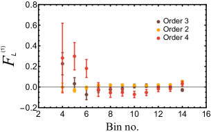
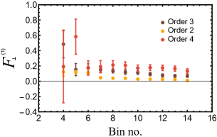
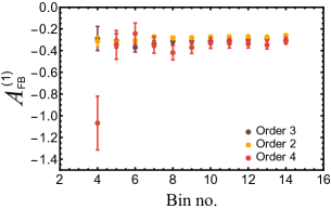
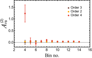
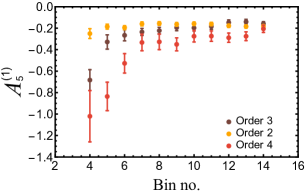
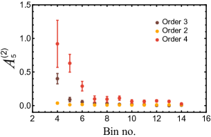
Figure 4: Systematic study of the coefficients of observables with the variation of polynomial order and the number of bins used for the fit. The color code for the different orders of the fitted polynomial is depicted in the panel. The $x$-axis denotes the number of bins used for the fit from last 4 to 14 bins. Coefficient values show good convergence within the $\pm 1\sigma$ error bars except for few bins in the $F_{\perp}^{(1)}$ and $A_{5}^{(1)}$ distributions.

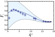
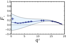
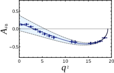
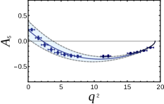
Figure 5: Fits with third order polynomials to the theoretical SM observables, generated using LCSR form factors for $q^{2}\leq 15\mathrm{\,Ge\kern-1.00006ptV}^{2}$ and Lattice QCD form factors for $q^{2}\geq 15\mathrm{\,Ge\kern-1.00006ptV}^{2}$.

V Convergence of Polynomial Fit

It is discussed in Sec. II the observables are Taylor expanded around the endpoint $q^{2}_{\scriptscriptstyle\text{max}}$ in Eqs. (26)– (29). In this section, we study the systematics of the fits to coefficients $F_{L}^{(1)}$, $F_{P}^{(1)}$, $A_{\text{FB}}^{(1)}$, $A_{\text{FB}}^{(2)}$, $A_{5}^{(1)}$ and $A_{5}^{(1)}$, which appear in the expressions of $\omega_{1}$ and $\omega_{2}$ given in Eq. (33). We vary the order the polynomial fitted from $2$ to $4$. Fits are also performed by varying the number of bins from the last $4$ to $14$ bins. The plots for the observables $A_{\text{FB}}$, $A_{5}$ $F_{L}$ and $F_{\perp}$ are shown in Appendix. C. The summary of the variation of fits with respect to the order of the polynomial and number of bins are given in Fig. 4 for all observable coefficients $F_{L}^{(1)}$, $F_{P}^{(1)}$, $A_{\text{FB}}^{(1)}$, $A_{\text{FB}}^{(2)}$, $A_{5}^{(1)}$ and $A_{5}^{(2)}$, respectively. The color code for the order of the polynomial used to fit is given in the panel. The $x-$ axis denotes the number of bins from last 4 to last 10 bins. We find that all the fitted coefficients show a good degree of convergence even when larger number of bins are added. The values obtained for the coefficients are consistent within $\pm 1\sigma$ regions apart from some small mismatches in $F_{P}^{(1)}$, and $A_{5}^{(1)}$. We choose as a benchmark the third order polynomial fit to all 14 bins.

To validate this choice of a third order polynomial fit to all 14 bins, we also perform an identical fit for observables generated using form factor values from LCSR [18] for the $q^{2}\leq 15\mathrm{\,Ge\kern-1.00006ptV}^{2}$ and from Lattice QCD [19] for $q^{2}\geq 15\mathrm{\,Ge\kern-1.00006ptV}^{2}$ region. The fits are shown in Fig. 5, where the blue error bars are bin integrated SM estimates and the solid blue curve with the shaded region represents the best fit polynomial with $\pm 1\sigma$ errors. The fits to SM observables are satisfactory for the entire $q^{2}$ region.

VI Conclusion

In conclusion, we have shown how RH currents can be uniquely probed without any hadronic approximations at $q^{2}_{\scriptscriptstyle\text{max}}$. Our approach adopted in Sec. II differs from other approaches [2] that probe new physics at low $q^{2}$, as it does not require estimates of hadronic parameters but relies instead on heavy quark symmetry based arguments that are reliable at $q^{2}_{\scriptscriptstyle\text{max}}$ [3, 4]. Our parameters are defined so as to notionally include non-factorizable loop correction and power-corrections and must differ from those of others. It should be noted that we use data directly, instead of theory estimates, to derive our conclusions. We understand that experimental measurements cannot alone result in discovery of NP as re-parameterization invariance suggests and to that end we rely on theoretical understanding of symmetries at the endpoint. While the observables themselves remain unaltered from their SM values, their derivatives and second derivatives at the endpoint are sensitive to NP effects. Large values of $A_{\text{FB}}$ and $A_{5}$, which do not rapidly approach zero in the neighborhood of $q^{2}_{\scriptscriptstyle\text{max}}$, are indicative of NP effects. In Sec. III we show that LHCb data implies $5\sigma$ evidence of NP at $q^{2}_{\scriptscriptstyle\text{max}}$. While the signal for right handed currents is clear, the large central values of $\xi$ and $\xi^{\prime}$ obtained will be reduced if other NP contributions are present. Allowing variation in the only input parameter i.e $r/C_{10}$, we obtain $3\sigma$ evidence of RH currents from the latest LHCb measurements. A detailed study of resonance effects has been carried out in Sec. IV, which provides more significant evidence for RH currents. The systematics of polynomial fit has been discussed in Sec.V where a good convergence has been observed when a large number of bins are considered. The choice of a particular polynomial parametrization has been justified with a fit to SM observables. The effect of complex contributions in the amplitudes (in Appendix A) and the finite ${K^{\!*}}$ width (in Appendix B) leaves the conclusions unchanged. In view of these, we speculate that if the current features of data persist with higher statistics the existence of RH currents can be established in the near future.

Appendix A Effect of Complex Contributions of amplitude

We show that the contributions arising from the complex part $(\varepsilon_{\lambda})$ of the amplitudes, in Eq. (3), can be incorporated in the following way.

Defining a new notation $\widehat{\varepsilon}_{\lambda}\equiv 2|\varepsilon_{\lambda}|^{2}/\Gamma_{f}$, the Taylor expansions for each $\widehat{\varepsilon}_{\lambda}$ around $q^{2}=q^{2}_{\scriptscriptstyle\text{max}}$ are given by,

$$\widehat{\varepsilon}_{\perp} =\widehat{\varepsilon}_{\perp}^{(1)}\delta+\widehat{\varepsilon}_{\perp}^{(2)}\delta^{2}+\widehat{\varepsilon}_{\perp}^{(3)}\delta^{3}$$

$$\widehat{\varepsilon}_{0} =\widehat{\varepsilon}_{0}^{(0)}+\widehat{\varepsilon}_{0}^{(1)}\delta+\widehat{\varepsilon}_{0}^{(2)}\delta^{2}$$

$$\widehat{\varepsilon}_{\|} =\widehat{\varepsilon}_{\|}^{(0)}+\widehat{\varepsilon}_{\|}^{(1)}\delta+\widehat{\varepsilon}_{\|}^{(2)}\delta^{2}$$

where $\delta\equiv q^{2}_{\scriptscriptstyle\text{max}}-q^{2}$ and the limiting values of helicity fractions, $F_{L}(q^{2}_{\scriptscriptstyle\text{max}})=1/3\text{~{}and~{}}F_{\|}(q^{2}_{\scriptscriptstyle\text{max}})=2/3$, constrain the coefficients i.e. $\widehat{\varepsilon}_{\|}^{(0)}=2\,\widehat{\varepsilon}_{0}^{(0)}$. The presence of complex amplitudes leads to a modification of the expressions of $\omega_{1}$ and $\omega_{2}$ (Eq. (33)) in the following way,

$$\omega_{1}=\, \displaystyle\frac{9}{4}\frac{\left(\frac{2}{3}-2\,\widehat{\varepsilon}_{0}^{(0)}\right)\left(F_{\perp}^{(1)}-\widehat{\varepsilon}_{\perp}^{(1)}\right)}{A_{\text{FB}}^{(1)\,2}}$$ (39)

$$\omega_{2}=\, \displaystyle\frac{4\,\Big{(}2A_{5}^{(2)}-A_{\text{FB}}^{(2)}\Big{)}\Big{(}1-3\,\widehat{\varepsilon}_{0}^{(0)}\Big{)}}{3\,A_{\text{FB}}^{(1)}\Big{(}3F_{L}^{(1)}+F_{\perp}^{(1)}+\widehat{\varepsilon}_{\|}^{(1)}-2\,\widehat{\varepsilon}_{0}^{(1)}\Big{)}}.$$ (40)

The procedure to incorporate the complex part of the amplitudes $\varepsilon_{\lambda}$ is described in Ref. [7], where it was shown that the complex part of the amplitudes $\varepsilon_{\lambda}$ are proportional to the asymmetries $A_{7}$, $A_{8}$ and $A_{9}$. Using $3\mbox{\,fb}^{-1}$ of LHCb data [14], we simulated values of the coefficients $\widehat{\varepsilon}_{0}^{(0)}$, $\widehat{\varepsilon}_{0}^{(1)}$, $\widehat{\varepsilon}_{\|}^{(1)}$ and $\widehat{\varepsilon}_{\perp}^{(1)}$; these turn out to be very small at the kinematic endpoint. These estimated coefficients are used to evaluate $\omega_{1}=1.03\pm 0.31~{}(0.98\pm 0.29)$ and $\omega_{2}=-4.52\pm 17.40~{}(-3.94\pm 9.86)$ (Eq. (39) and (40)), where the first values are determined using $A_{\text{FB}}^{(1)}$ and $A_{9}^{(1)}$ whereas the values in the round brackets use $2A_{5}^{(1)}$ and $-\frac{2}{3}A_{8}^{(1)}$. The factorization assumption is needed only at leading order in the expansions of observables, which requires $A_{\text{FB}}^{(1)}=2A_{5}^{(1)}$ and $A_{9}^{(1)}=-\frac{2}{3}A_{8}^{(1)}$.

It should be noted that the inclusion of $\widehat{\varepsilon}_{\lambda}$’s change the values of $\omega_{1}$ and $\omega_{2}$ insignificantly, with corresponding estimates for the real case being well within the $\pm 1\sigma$ errors. Hence, the conclusions derived in the paper are robust against the inclusion of complex contributions in the amplitudes.

Appendix B Finite ${K^{\!*}}$ width effect

The finite width of the ${K^{\!*}}$ can alter the position of the kinematic endpoint i.e $q^{2}_{\scriptscriptstyle\text{max}}$ value. As LHCb considers a much wider range for the width of $K^{*}$, compared to the observed width (which is $\sim 50$ MeV), we have varied the $q^{2}_{\scriptscriptstyle\text{max}}$ value in the Taylor expansion of observables (Eqs. (26)–(29)) within an interval $18.34-20.10$ GeV². The observables $\omega_{1}$ and $\omega_{2}$ are evaluated for each case and a weighted average over the Breit-Wigner shape for a ${K^{\!*}}$ gives $\omega_{1}=1.11\pm 0.30~{}(1.03\pm 0.35)$ and $\omega_{2}=-3.56\pm 28.34~{}(-3.50\pm 27.44)$. The change in the values of $\omega_{1}$ and $\omega_{2}$ have an insignificant effect in Fig. 1 and 2 and the results derived in this work.

Appendix C Polynomial fit variation

The variation of fits with respect to the order of the polynomial and number of bins are shown in Fig. 6, 7, 8 and 9 for observables $A_{\text{FB}}$, $A_{5}$, $F_{L}$ and $F_{\perp}$, respectively The color code is the same as in Fig. 1. The panel in each plot depicts the number of bins (from kinematic endpoint) and the order of polynomial is used for the fit. The extracted coefficient values of the observables from these plots are summarized in Fig. 5.

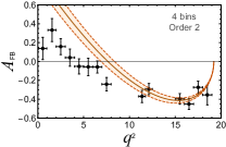
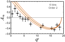
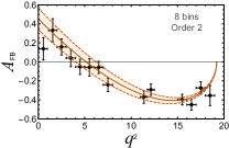
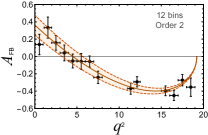
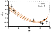
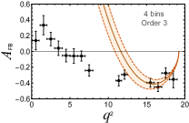
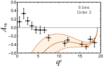
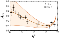
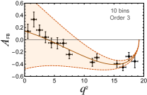
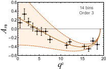
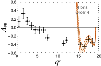
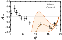
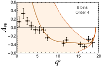
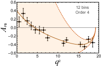
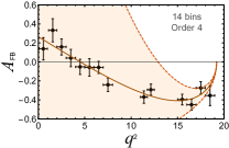
Figure 6: Fits to $A_{\text{FB}}$ using various numbers of bins and polynomial parameterizations. The color code is the same as in Fig. 1

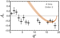
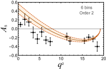
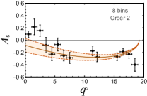
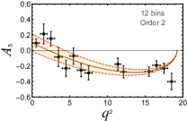
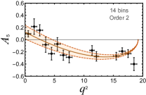
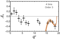
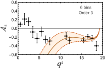
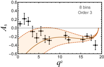
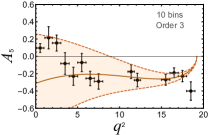
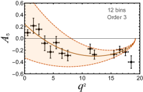
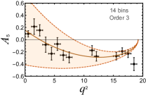
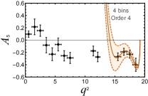
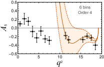
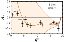
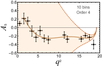
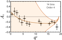
Figure 7: Fits to $A_{5}$ various numbers of bins and polynomial parameterizations. The color code is the same as in Fig. 1

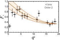
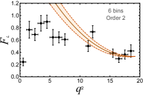
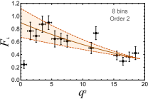
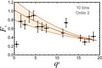
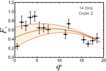
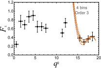
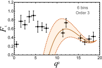
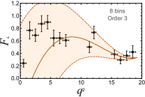
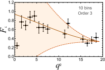
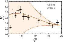
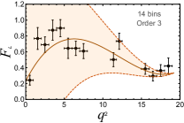
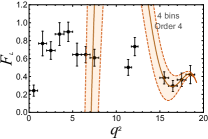
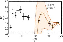
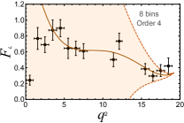
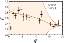
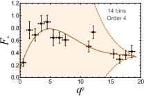
Figure 8: Fits to $F_{L}$ various numbers of bins and polynomial parameterizations. The color code is the same as in Fig. 1

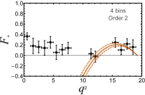
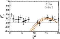
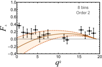
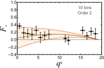
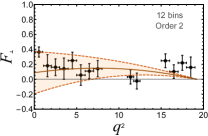
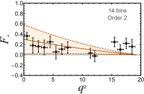
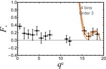
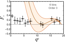
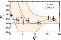
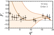
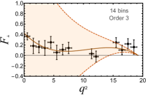
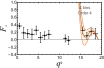
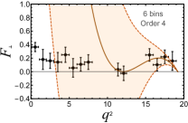
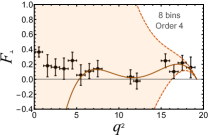
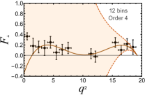
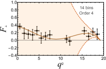
Figure 9: Fits to $F_{\perp}$ various numbers of bins and polynomial parameterizations. The color code is the same as in Fig. 1

References

• [1] F. Kruger, L. M. Sehgal, N. Sinha, R. Sinha, Phys. Rev.  D61, 114028 (2000). [hep-ph/9907386].
• [2] W. Altmannshofer and D. M. Straub, Eur. Phys. J. C 75, no. 8, 382 (2015); M. Ciuchini et al. JHEP 1606, 116 (2016). S. Jäger and J. Martin Camalich, Phys. Rev. D 93 (2016) 1, 014028; S. Descotes-Genon, J. Matias and J. Virto, Phys. Rev. D 88, 074002 (2013) [arXiv:1307.5683 [hep-ph]]. S. Descotes-Genon, L. Hofer, J. Matias and J. Virto, JHEP 1606, 092 (2016) and references therein.
• [3] B. Grinstein, D. Prijol, Phys. Rev.  D 70 114005 (2004).
• [4] C. Bobeth, G. Hiller and D. van Dyk, Phys. Rev. D 87 (2013) 3, 034016
• [5] R. Mandal and R. Sinha, arXiv:1506.04535 [hep-ph].
• [6] G. Hiller, Roman Zwicky, JHEP 1403, 042 (2014).
• [7] R. Mandal, R. Sinha and D. Das, Phys. Rev. D 90, no. 9, 096006 (2014)
• [8] The lepton mass corrections can easily be included as shown in Ref. [7]. However the corrections are negligible at large $q^{2}$.
• [9] M. Beneke, T. Feldmann, D. Seidel, Nucl. Phys.  B612, 25-58 (2001). [hep-ph/0106067];
• [10] A. Khodjamirian, T. Mannel, A. A. Pivovarov and Y.-M. Wang, JHEP 1009, 089 (2010).
• [11] W. Altmannshofer, P. Ball, A. Bharucha et al., JHEP 0901, 019 (2009). [arXiv:0811.1214 [hep-ph]].
• [12] C. Bobeth, G. Hiller and D. van Dyk, JHEP 1007, 098 (2010).
• [13] D. Das and R. Sinha, Phys. Rev. D 86 (2012) 056006 [arXiv:1205.1438 [hep-ph]];
• [14] R. Aaij et al. [LHCb Collaboration], JHEP 1602, 104 (2016).
• [15] R. Aaij et al. [LHCb Collaboration], arXiv:1606.04731 [hep-ex].
• [16] F. Beaujean, M. Chrzäszcz, N. Serra and D. van Dyk, Phys. Rev. D 91, 114012 (2015).
• [17] J. Lyon and R. Zwicky, arXiv:1406.0566 [hep-ph].
• [18] A. Bharucha, D. M. Straub and R. Zwicky, JHEP 1608, 098 (2016) [arXiv:1503.05534 [hep-ph]].
• [19] R. R. Horgan, Z. Liu, S. Meinel and M. Wingate, Phys. Rev. Lett.  112, 212003 (2014); [arXiv:1310.3887 [hep-ph]]; R. R. Horgan, Z. Liu, S. Meinel and M. Wingate, arXiv:1501.00367 [hep-lat].
• [20] F. Kruger and L. M. Sehgal, Phys. Lett. B 380, 199 (1996) [hep-ph/9603237].
• [21] K. A. Olive et al. [Particle Data Group Collaboration], Chin. Phys. C 38, 090001 (2014).
• [22] R. Aaij et al. [LHCb Collaboration], Phys. Rev. D 86, 071102 (2012) [arXiv:1208.0738 [hep-ex]].
• [23] K. Abe et al. [Belle Collaboration], Phys. Lett. B 538, 11 (2002) [hep-ex/0205021].
• [24] http://www.imsc.res.in/$\sim$abinashkn/arXiv
• [25] K. De Bruyn, R. Fleischer, R. Knegjens, P. Koppenburg, M. Merk, A. Pellegrino and N. Tuning, Phys. Rev. Lett.  109, 041801 (2012) [arXiv:1204.1737 [hep-ph]].