Constructing multiscale gravitational energy spectra from molecular cloud surface density PDF – Interplay between turbulence and gravity

Abstract

Gravity is believed to be important on multiple physical scales in molecular clouds. However, quantitative constraints on gravity are still lacking. We derive an analytical formula which provides estimates on multiscale gravitational energy distribution using the observed surface density PDF. Our analytical formalism also enables one to convert the observed column density PDF into an estimated volume density PDF, and to obtain average radial density profile $\rho(r)$. For a region with $N_{\rm col}\sim N^{-\gamma_{\rm N}}$, the gravitational energy spectra is $E_{\rm p}(k)\sim k^{-4(1-1/\gamma_{\rm N})}$. We apply the formula to observations of molecular clouds, and find that a scaling index of $-2$ of the surface density PDF implies that $\rho\sim r^{-2}$ and $E_{\rm p}(k)\sim k^{-2}$. The results are valid from the cloud scale (a few parsec) to around $\sim 0.1\;\rm pc$. Because of the resemblance the scaling index of the gravitational energy spectrum and the that of the kinetic energy power spectrum of the Burgers turbulence (where $E\sim k^{-2}$), our result indicates that gravity can act effectively against turbulence over a multitude of physical scales. This is the critical scaling index which divides molecular clouds into two categories: clouds like Orion and Ophiuchus have shallower power laws, and the amount of gravitational energy is too large for turbulence to be effective inside the cloud. Because gravity dominates, we call this type of cloud g-type clouds. On the other hand, clouds like the California molecular cloud and the Pipe nebula have steeper power laws, and turbulence can overcome gravity if it can cascade effectively from the large scale. We call this type of cloud t-type clouds. The analytical formula can be used to determine if gravity is dominating cloud evolution when the column density probability distribution function (PDF) can be reliably determined.

1 Introduction

The interplay between turbulence and gravity plays determining roles in the dynamics of astrophysical fluids, and in particular molecular clouds (Dobbs et al., 2014, and references therein). Turbulence is a self-similar process. It is believed that it can effectively transport energy from the large scale to smaller scales, and provide necessary support to stop matter from collapsing too rapidly (Mac Low & Klessen, 2004). The effect of turbulence in star formation is subject to intensive investigations during the past decade (see e.g. Ballesteros-Paredes et al. (2007) and references therein).

Gravity, being the only long-range and attractive force, determines the dynamics of the majority of astrophysical systems. Molecular clouds exhibit structures on a multitude of physical scales – from at least $10^{2}$ parsec down to sub-parsec scales (Williams et al., 2000). Because gravity is scale-free, it can be important on all these physical scales. Previously, the importance of gravity has been quantified on various scales using the virial parameter (Bertoldi & McKee, 1992). The importance of gravity on multiple physical scales has also been observationally demonstrated (Goodman et al., 2009; Li et al., 2015b). One limitation of the virial parameter is that one needs to specify a scale on which it can be evaluated. Thus it is difficult to obtain a multiscale picture of gravity based on the virial parameter alone. Besides, the virial parameter is not additive. Thus it is not useful for evaluating the importance of gravity on bulk molecular gas.

A better representation of the importance of gravity is the gravitational energy. Compared to the virial parameter, energy is additive. One can separate the total gravitational energy of a molecular cloud into contributions from different parts and from different physical scales. This provides a multiscale picture of gravity in molecular clouds – an important piece of information that is still missing. This task is now feasible as observations can reliably trace the gas from $10^{2}$ parsec down to sub-parsec scales e.g. Schneider et al. (2013, 2012); Kainulainen et al. (2009); Lombardi et al. (2015).

The structure of a molecular cloud can be interpreted by the surface density PDFs (PDF is the probability distribution function). It is a measure of the distribution of the observed surface density structure of a molecular cloud. Observationally, the PDFs are found to exhibit power-law forms $P_{\rm N_{\rm col}}\sim N_{\rm col}^{-\gamma_{\rm N}}$ (Lombardi et al., 2015; Schneider et al., 2013, 2012; Kainulainen et al., 2009; Lombardi et al., 2015; Kainulainen et al., 2014), at least for the parts with high surface densities (Kainulainen et al., 2009). This is usually interpreted as the system being strongly self-gravitating, perhaps also influenced by rotation and magnetic field (Kritsuk et al., 2011; Girichidis et al., 2014; Kainulainen et al., 2009). We note, however, that power-law PDFs has been noticed in other some earlier simulations. See e.g. Scalo et al. (1998); Federrath et al. (2008); Vázquez-Semadeni et al. (2008); Klessen (2000); Collins et al. (2011). One importance piece of information that one can extract from an observed surface density PDF is to constrain how the gravitational energy of a molecular cloud is distributed across different physical scales. This is the major focus of this work .

We present observational constraints on the multiscale importance of gravity by inferring it from the observed surface density PDF of a molecular cloud. The formalism is based on a simple view, that the high-density parts of the gas tend to be surrounded by gas of relatively lower densities. This insight enables us to construct a nested shell model for the dense parts of molecular clouds. The model characterises the structures seen in observations and yet at the same time enables us to evaluate the contribution to the gravitational energy from various physical scales with an analytical approach. The paper is organized as follows: In Section 2 we describe our model, and derive an analytical formula to compute the multiscale gravitational energy distribution (called gravitational energy spectrum in this work) from the observed surface density PDF. The formulas to convert the observed column density PDF into volume density PDF, averaged radial profile and gravitational energy spectra are summarized in Sec. 2.4. Then these formulas are applied to observations to provide constraints (Sec. 3). In Sec. 4 we conclude.

2 multiscale gravitational energy

2.1 Observational picture

A surface density PDF is a statistical probability distribution of the observed surface densities of a molecular cloud. At high surface densities, molecular clouds exhibit power-law PDFs. It has been demonstrated that one can “unfold” the observed surface density distribution into the intrinsic density PDF ($\rho$-PDF, (Kainulainen et al., 2014)), either with a volume density modelling technique (Kainulainen et al., 2014) or with an analytical formula (Girichidis et al., 2014; Kritsuk et al., 2011; Federrath & Klessen, 2013; Brunt et al., 2010).

Suppose that above a critical surface density of $N_{\rm col,\ min}$, a molecular cloud has an observed surface density distribution of

$$P(N_{\rm col})=P_{N_{0}}\Big{(}\frac{N_{\rm col}}{N_{0}}\Big{)}^{-\gamma_{\rm N}}\;,$$ (1)

where $N_{\rm col}$ is the observed surface density and $\gamma_{\rm N}\approx 2$. This is a fiducial value, and observationally, different clouds have very different slopes. For star-forming cloud, $\gamma_{\rm N}$ can reach 1.5; for non-star-forming clouds, $\gamma_{\rm N}\approx 4$. The range of scaling exponents has been seen in both extinction-based observations e.g. (Kainulainen et al., 2009) and in emission-based measurements e.g. (Schneider et al., 2012; Lombardi et al., 2014). See also Table 1. The $\rho$-PDF can be estimated as (Girichidis et al., 2014)

$$P(\rho)=P_{\rho_{0}}\Big{(}\frac{\rho}{\rho_{0}}\Big{)}^{-\gamma_{\rho}}\;,$$

where

$$\gamma_{\rho}=\frac{3\gamma_{\rm N}}{\gamma_{\rm N}+2}\;.$$ (2)

where $\rho_{0}\approx N_{0}/L$ and $L$ is the size of the region. The normalization depends on $L$, which one can measure form the images, and the normalization is accurate only in order-of-magnitude sense. As a crude estimate, $L\approx\sqrt{P_{N_{0}}}{\rm d}x$ where ${\rm d}x$ is the pixel size. On the 2D plane, the region is composed of $M\approx N\times N=(L/{\rm d}x)^{2}$ pixels which implies $P_{N_{0}}\approx L^{2}$, and in 3D, the region is composed of $M^{\prime}\approx N\times N\times N=(L/{\rm d}x)^{3}$ vorxels, which implies $P_{\rho_{0}}\approx L^{3}$. Here, $P_{N_{0}}$ and $P_{\rho_{0}}$ have dimensions of area and volume, respectively. As has been demonstrated in Girichidis et al. (2014); Kritsuk et al. (2013); Fischera (2014), this empirical relation is reasonably accurate when applied to numerical simulations where a multitude of structures are present.

2.2 The shell model

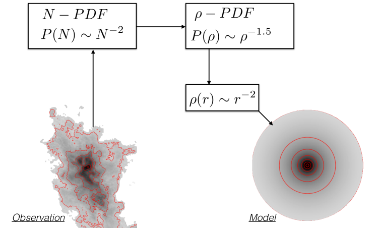
Figure 1: A illustration of the model. For a given star-forming region (e.g. the NGC1333 star forming region as has been shown on the left), we can constraint is surface density PDF (N-PDF) observationally. Then we can construct a volume density PDF ($\rho$-PDF) based on the surface density PDF. Finally, we construct a shell model where the density distribution can be described as the effective radial profile $\rho(r)\sim r^{-2}$ where $r$ is the radius. This is an approximation to the real density structure of the region. Turbulence can be driven from the outer shell and would cascades inwards. The image of NGC1333 (on the left) is produced from the velocity-integrated ¹³CO(1-0) data from the COMPLETE survey (Ridge et al., 2006). The image on the right is produced with the an analytical formula, which can be found in the clump model section of Li et al. (2016a). The conversion between density PDF and effective radial density profiles can be found in Sec. 2.4.

We assume a multiscale spherical symmetric nested model for molecular clouds where gas with high densities stays inside regions of lower densities. We consider a simplified model where the entire star-forming region can be approximated as one such structure. We call this a “shell model”. The basic idea of this simplification is sketched in Fig. 1.

We assume that above a critical density $\rho_{\rm crit}$, a star-forming region obeys

$$P(\rho)=P_{\rho_{0}}\times\Big{(}\frac{\rho}{\rho_{0}}\Big{)}^{-\gamma_{\rho}}\;,$$ (3)

where a fiducial value of $\gamma_{\rho}$ woudl be $1.5$. $P_{\rho_{0}}\approx L^{3}$ where $L$ is the size of the region, and $\rho_{0}\approx N_{0}/L$. Here, the probability is measured in terms of surface area, and $P_{\rho_{0}}$ has a unit of $L^{3}$ where $L$ is the size. The amount of mass ${\rm d}M(\rho)$ contained in a shell of mass with $(\rho,\rho+{\rm d}\rho)$ is

$${\rm d}M(\rho)=P(\rho){\rm d}\rho=P_{\rho_{0}}\times\Big{(}\frac{\rho}{\rho_{0}}\Big{)}^{-\gamma_{\rho}}{\rm d}\rho$$ (4)

and the enclosed mass inside such a shell is

$$M_{\rm enc}(\rho) = \int_{\rho}^{\rho_{\rm max}}P(\rho^{\prime}){\rm d}\rho^{\prime}$$

$$= P_{\rho_{0}}\rho_{0}\frac{(\rho^{\prime}/\rho_{0})^{1-\gamma_{\rho}}}{1-\gamma_{\rho}}\Big{|}^{\rho_{\rm max}}_{\rho}=\frac{P_{\rho_{0}}\rho_{0}}{\gamma_{\rho}-1}\Big{(}\frac{\rho}{\rho_{0}}\Big{)}^{1-\gamma_{\rho}}\;$$

where in the last step we assume $\gamma_{\rho}>1$ and $\rho_{\rm max}\gg\rho$. For simplicity, factors that are of order 1 such as $1-\gamma_{\rho}$ are dropped from further analysis. Note that $\gamma_{\rho}>1$ is a necessary condition for the integration to converge (which correspond to $\gamma_{\rm N}>1$). This is in generally satisfied for the observed star-forming regions (Kainulainen et al., 2014; Stutz & Kainulainen, 2015), and can be understood theoretically (Kritsuk et al., 2011).

The mass of the region can be estimated using the shell approximation

$${\rm d}M(\rho)\approx 4\pi r^{2}\,\rho{\rm d}r\;,$$ (6)

from which we derive (using $r\rightarrow 0$ when $\rho$ is sufficiently large) .

$$r(\rho)=\big{(}\frac{P_{\rho_{0}}}{4\pi}\big{)}^{\frac{1}{3}}\big{(}\frac{\rho}{\rho_{0}}\big{)}^{-\frac{\gamma_{\rho}}{3}}\;,$$ (7)

which is

$$\rho=\rho_{0}\,\big{(}\frac{P_{\rho_{0}}}{4\pi}\big{)}^{\frac{1}{\gamma_{\rho}}}r^{-\frac{3}{\gamma_{\rho}}}=\rho_{0}\,\big{(}\frac{P_{\rho_{0}}}{4\pi}\big{)}^{\frac{1}{\gamma_{\rho}}}r^{-(1+\frac{2}{\gamma_{\rm N}})}\;.$$ (8)

Observations have found that $\gamma_{\rm N}\approx 2$ which implies $\rho\sim r^{-2}$ (see also Kritsuk et al. (2011); Kainulainen et al. (2014); Fischera (2014); Federrath & Klessen (2013)).

2.3 multiscale gravitational energy

The gravitational binding energy of one single shell is

$$E_{\rm p}^{\rm shell}=\frac{GM_{\rm enc}(\rho)\;{\rm d}M(\rho)}{r(\rho)}\;,$$ (9)

it can be simplified using Equations 4, 2.2 and 7, where factors such $4\pi$ are omitted for simplicity

$$E_{\rm p}^{\rm shell}\approx\,G\,P_{\rho_{0}}^{\frac{5}{3}}\,\rho_{0}\Big{(}\frac{\rho}{\rho_{0}}\Big{)}^{1-\frac{5}{3}\gamma_{\rho}}{\rm d}\rho\;,$$ (10)

and

$$E_{\rm p}^{\rm shell}(r)\approx G\;P_{\rho_{0}}^{\frac{1}{\gamma_{\rho}}}\,\rho_{0}\;r^{\frac{4\gamma_{\rho}-6}{\gamma_{\rho}}}|{\rm d}r|\;.$$ (11)

Defining the wavenumber $k=2\pi/r$, following the convention used in turbulence studies (Frisch, 1995), the gravitational energy spectrum of the system is,

$$E_{\rm p}(k)=\Big{|}\frac{{\rm d}E_{\rm p}^{\rm shell}(k)}{{\rm d}k}\Big{|}\approx G\;P_{\rho_{0}}^{\frac{1}{\gamma_{\rho}}}\,\rho_{0}k^{\frac{-6(\gamma_{\rho}-1)}{\gamma_{\rho}}}\;,$$ (12)

where $E_{\rm p}(k)$ has a unit that is the same as the turbulence power spectrum $E_{\rm turb}(k)$. Using Eq. 2, we can express it as a function of the scaling exponent $\gamma_{\rm N}$ of the surface density PDF (where $P(N)\sim N_{\rm col}^{-\gamma_{\rm N}}$)

$$E_{\rm p}(k)\approx G\;P_{\rho_{0}}^{\frac{\gamma_{\rm N}+2}{3\gamma_{\rm N}}}\,\rho_{0}\;k^{-4(1-\frac{1}{\gamma_{\rm N}})}\sim k^{-4(1-\frac{1}{\gamma_{\rm N}})}\;.$$ (13)

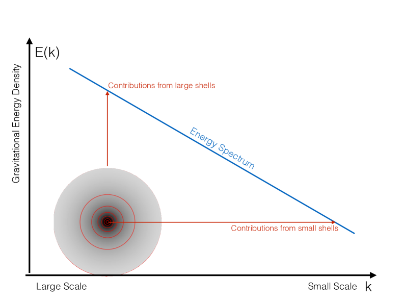
Figure 2: A illustration of the concept of gravitational energy spectrum. The image on the bottom left is produced from an idealised cloud, where we divide it into a set of nested shells. The boundaries of the shells are marked by the red contours. The formula for making this density structure can be found in the clump model section of Li et al. (2016a). The gravitational energy spectrum is the distribution of the total gravitational energy of the cloud at different wavenumbers $k$ where $k$ is related to the physical scale by $k=2\pi/l$. A large $k$ represents the gravitational energy at a small scale, contributed from gas that resides in the inner parts of the region. A small $k$ represent the gravitational energy at a large scale, contributed by gas at the outer envelopes. See Sec. 2.3 for details.

Here we briefly explain the meaning of the formula for the gravitational energy spectrum (Eq. 13). The gravitational energy spectrum is the distribution of the total gravitational energy of the cloud at different wavenumbers $k$ where $k$ is related to the physical scale by $k=2\pi/l$. A large $k$ represents the gravitational energy at small scales, contributed by gas that resides in the inner parts of the region. A small $k$ represents the gravitational energy at large scales, contributed by gas at the outer envelopes. A steeper slope of $E_{\rm p}(k)$ means gravitational energy is concentrated at larger scales, and a shallower slope means gravitational energy is concentrated at smaller scales. This is illustrated in Fig. 2.

The energy spectrum satisfies energy conservation

$$\int E_{\rm p}(k){\rm d}k=\int E_{\rm p}(r){\rm d}r=E_{\rm p}^{\rm tot}\;,$$ (14)

where $E_{\rm p}^{\rm tot}$ is the total gravitational binding energy of the system. Here we prefer to use the wavenumber $k$ over the size $l$ as the gravitational energy spectrum should have an identical form to the turbulent kinetic energy spectrum $E_{\rm turb}(k)$.

2.4 Conversion between N-PDF, $\rho$-PDF and $\rho(r)$ and $E_{\rm p}(k)$

The formalism described above enables us to convert the observed N-PDF into $\rho$-PDF and finally into the density profile $\rho(r)$ and derive the gravitational energy spectrum $E_{\rm p}(k)$. This enables the observers to interpreted the observed surface density PDF with physically meaningful models. For this purpose, we collected all the useful formulas below. These formula are accurate in order-of-magnitude sense. Suppose we have a region of size $L$, and this region has a minimum surface density $N_{0}$. In this region, the high surface density part stays inside envelopes of low surface densities (like the case of NGC1333 shown in Fig. 1), and its N-PDF can be written as

$$P(N_{\rm col})=L^{2}\Big{(}\frac{N_{\rm col}}{N_{0}}\Big{)}^{-\gamma_{\rm N}}\;,$$ (15)

where $N_{0}$ is a critical surface density. According to the shell model, its $\rho$-PDF is (from Eq. 3)

$$P(\rho)=L^{3}\times\Big{(}\frac{\rho}{\rho_{0}}\Big{)}^{-\gamma_{\rho}}\;,$$ (16)

where $\rho_{0}\approx N_{0}/L$ and $\gamma_{\rho}$ is given by Eq. 2. One can derive the radial density profile (from Eq. 8):

$$\rho(r)=\rho_{0}\,L^{\frac{3}{\gamma_{\rho}}}r^{-(1+\frac{2}{\gamma_{\rm N}})}\;.$$ (17)

The gravitational energy spectrum of the system is (from Eq. 13)

$$E_{\rm p}(k)\approx G\;L^{\frac{\gamma_{\rm N}+2}{\gamma_{\rm N}}}\,\rho_{0}\;k^{-4(1-\frac{1}{\gamma_{\rm N}})}\sim k^{-4(1-\frac{1}{\gamma_{\rm N}})}\;.$$ (18)

2.5 Uncertainty from the underlying geometry of the gas

Star-forming regions are known to be irregular, having substructures. In our simplified shell model, the cloud is approximated as a collection of nested shells. This will introduce some inaccuracies in the estimate of gravitational energy. Here we briefly discuss this accuracy issue.

We consider a thought experiment where we artificially split an object into $N$ completely separated identical sub-clumps and keep the density distribution unchanged. The gravitational energy of an object of mass $M$ and size $r_{0}$ is

$$E_{0}=\eta\frac{GM^{2}}{r_{0}}\;,$$ (19)

where $\eta\sim 1$ and is dependent on the underlying geometry of the gas. After the artificial fragmentation, this object is divided into $N$ smaller objects of equal mass of $M/N$ and equal radius $r_{0}/N^{1/3}$. The total gravitational energy of the artificially fragmented system is

$$E_{1}=\eta\frac{G(M/N)^{2}\times N}{r/N^{1/3}}=E_{0}N^{-2/3}\;.$$ (20)

Thus this artificial fragmentation process will decrease the gravitational binding energy by a factor of $N^{-2/3}$ where $N$ is the number of subregions.

The energy difference created by this artificial splitting (fragmentation) process can be considered as a safe upper limit to the error of the estimation in reality. This is because in our calculations, after the artificial fragmentation experiment, the clumps are assumed to be gravitationally non-interacting. But in reality they are gravitationally interacting. This will decrease the energy difference between $E_{0}$ and $E_{1}$. Practically speaking, in many cases, we are interested in the general slope of the gravitational energy spectrum, as it tells us how the gravitational energy evolves with scale. In these cases, $N$ only influences the normalization of the gravitational energy spectrum, and does not change the slope.

Typically (see Fig. 3), for compact star forming regions like NGC1333 in the Perseus molecular cloud, the high density parts always stay inside nested envelopes of lower densities. Therefore $N\approx 1$ provides a fairly good description of the geometrical structure of such regions. For the Ophiuchus molecular cloud, fragmentation occurs, however, because the fragments are still close to each other spatially, and are probably interacting with each other gravitationally, we expect our model to be accurate. For regions like the Perseus, ideally, one could separate it into into subregions (e.g. NGC1333, B1, B2 and IC348) and evaluate the surface density PDFs and gravitational energy spectra for these regions. Alternative, by assume that these regions are almost identical, Eq. 13 can still be used to derive the slope of the gravitational energy spectrum. In this case, the normalization should be modified according to Eq. 20. Clouds like the Polaris molecular cloud are composed of many sub-regions. Here, one can still separate the cloud into individual subregions and evaluate the gravitational energy spectra of these regions, respectively. However, it is more convenient to use Eq. 13 to derive the gravitational energy spectrum of the cloud as a whole. In this case, it is implicitly assumed that these regions have somewhat similar shapes.

The geometry of star-forming regions are not symmetric, and filamentary structures has been seen on almost all scales . This might also be a contributing factor to the inaccuracy of the model. However, a detailed calculation suggests that this effect is not significant. The simplest way to quantify this is to consider the impact of aspect ratio on the estimated gravitational energy. An aspect ratio of $\sim 10$ only changes the gravitational binding energy by a factor of $\sim 1.5$ (see Appendix A for details). Thus our Equation 12 should be a good approximation of the energy spectrum in spite of all the above-mentioned compilations. When the regions are too complicated to be approximated with the shell model, one can also construct the gravitational energy spectrum numerically (see an accompanying paper, (Li & Burkert, 2016b)). In fact, using data from the Orion molecular cloud, Li & Burkert (2016b) demonstrated that the shell model appears to be a good approximation.

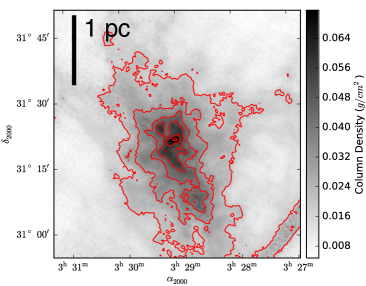
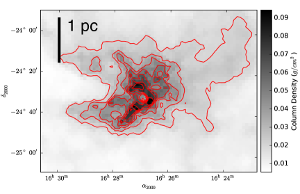
Figure 3: Surface density map of two star-forming regions. The NGC1333 region is displayed on the left panel. The surface density map is produced from the ¹³CO(1-0) map, using a conversion of $n_{\rm H_{2}}=5\times 10^{20}\rm\;(K\;\rm km/s)^{-1}$. The Ophiuchus star-forming region is displayed on the right panel. The surface density is estimated from extinction, using $n_{\rm H_{2}}=9\times 10^{20}\;A_{\rm v}^{-1}$ using COMPLETE (Ridge et al., 2006) data. The complexities of these regions can be seem from the wedged contours that traces the surface density distributions. High density regions tend to reside in envelopes of lower densities. This feature is captured in our model.

3 Interplay between turbulence and gravity

3.1 Observational results

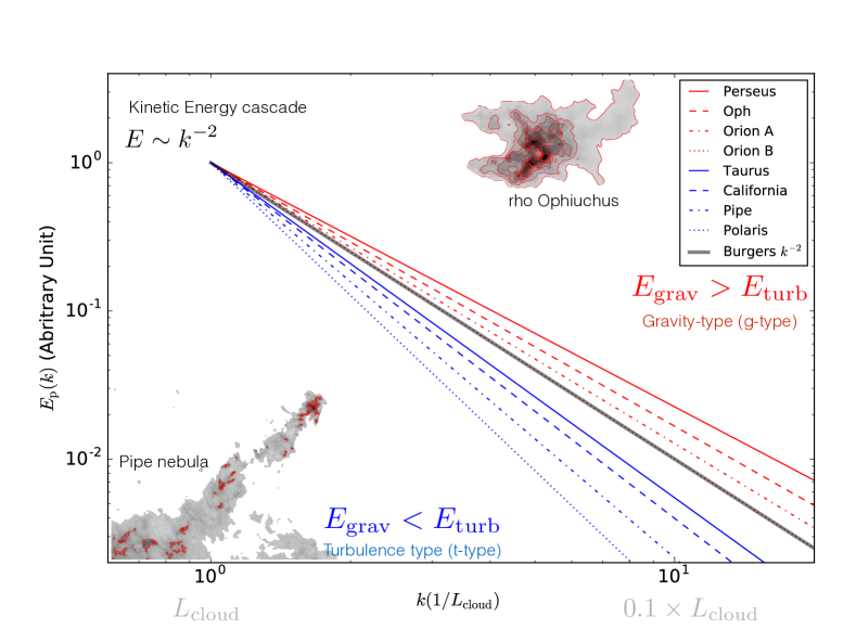
Figure 4: The derived gravitational energy spectra of several molecular clouds. The energy spectra are derived from Table 1 of Lombardi et al. (2015) (see also our Table 1), using Eq. 13. Gravitational energy at smaller scales (large $k$) is contributed by the inner shells, and gravitational energy at larger scales (small $k$) is contributed by the outer shells. The $x$-axis is normalized to the size of the cloud $L_{\rm cloud}$ (which is around a few parsec in size). The derived gravitational energy spectra are valid from the cloud scale to the map resolution (which is better than $0.1\,L_{\rm cloud}$ in our case). The normalization of the $y$-axis is arbitrary. Critical energy spectrum of Burgers turbulence $E(k)\sim k^{-2}$ is indicated by the thick black line. The gravitational energy spectrum of the Orion B cloud have $E(k)\sim k^{-2}$ and coincides with that of Burgers turbulence. Above the critical energy spectrum, the gravitational energy exceeds the inferred turbulence energy and gravitational collapse dominates. Below it, gravity can be balanced by turbulence. The embedded maps of the Pipe nebula (represent our t-type cloud ) is produced using the extinction data of Rowles & Froebrich (2009) and the $\rho$-Ophiuchus data (representing our g-type cloud) is from Ridge et al. (2006). For clarity, we have chosen a normalization such that the lines overlap at $L_{\rm cloud}$.

It has been demonstrated observationally that beyond a threshold column density, molecular clouds exhibit power-law PDFs (Kainulainen et al., 2009, 2011). Lombardi et al. (2015) studied the surface density distribution of 8 nearby molecular clouds, and argue that the threshold surface density extends down to $A_{\rm k}\gtrsim 0.3$, which is lower than the value found in Kainulainen et al. (2009, 2011). Different regions have different scaling indexes. We use these scaling indexes to determine the gravitational energy spectra of the clouds.

3.2 Two regimes of cloud evolution

It is found that turbulence in molecular clouds is supersonic. The power spectrum of the turbulence is believed to be close to that of Burgers turbulence, which is $E_{\rm k}\sim k^{-2}$ (Federrath, 2013). This is the maximum amount of energy one would expect to be transferred to smaller scales from turbulence cascade. On the largest scale, molecular clouds are close to be gravitational bound (Roman-Duval et al., 2010; Heyer et al., 2009), and the amount of turbulence energy is comparable to the gravitational binding energy. We note that there is still a large uncertainty (0.5 – 5) concerning the estimated virial parameters in the literature (Rosolowsky et al., 2007; Hernandez & Tan, 2015). Li et al. (2015b) have demonstrated that by carefully choosing the boundaries of the regions, the cloud is much more gravitationally bound what is suggested by a simple virial analysis. It remains to be investigated (following Li et al. (2015b)) if these uncertainties arise because of the chosen boundaries of the cloud, or the cloud are intrinsically unbound. Many of the clumps in the clouds are in virial equilibrium (Wienen et al., 2012). The importance of gravity in massive star-forming clumps has also been observationally demonstrated using the $\alpha_{vir}-\alpha_{G}$ formalism (Traficante et al., 2015).

At high surface density, it has been noticed that the surface density PDF of molecular clouds can be described by power-laws (Schneider et al., 2013, 2012; Kainulainen et al., 2009). With an almost-homogeneous sample of 8 molecular clouds, Lombardi et al. (2015) found that the power-law surface density PDFs starts at at $A_{\rm v}\gtrsim 0.3$. The derived scaling exponents are scatters around -2. Using Equation 13, this corresponds to a gravitational energy spectrum of $E_{\rm p}\sim k^{-2}$, which coincides exactly with the energy spectrum of Burgers turbulence. In this case, if turbulence can cascade effectively, the cloud should be in a critical state where the turbulence and gravitational energy are comparable on multiple scales (from a few parsec to subparsec). A steeper gravitational energy spectrum means that there is less gravitational energy than turbulent energy; and a shallower spectrum implies the dominance of gravitational energy.

In Fig. 4 we present the derived gravitational energy spectra using the results from Table 1 of Lombardi et al. (2015). The results are valid from $A_{\rm k}\approx 0.3$ to $A_{\rm k}\lesssim 10$. The gravitational energy spectra are evaluated using Eq. 13.

Region Name	$\gamma_{\rm N}$	$\gamma_{\rho}$	$\gamma_{\rm E_{\rm p}}$
Perseus	1.7	1.38	1.65
Oph	1.8	1.42	1.78
Orion A	1.9	1.46	1.89
Orion B	2.0	1.50	2.0
Taurus	2.3	1.60	2.26
California	2.5	1.67	2.4
Pipe	3.0	1.80	2.66
Polaris	3.9	1.98	2.97

Table 1: Properties of different regions. $\gamma_{\rm N}$ is the scaling exponent of the observed surface density PDF ($P(N_{\rm col})\sim N_{\rm col}^{-\gamma_{\rm N}}$ where $N_{\rm col}$ is the observed surface density). $\gamma_{\rho}$ is the scaling exponent of the theoretically-derived volume density PDF ($P(\rho)\sim\rho^{-\gamma_{\rm\rho}}$). $\gamma_{\rm E_{\rm p}}$ is the scaling exponent of the gravitational energy spectra ($E_{\rm p}(k)\sim k^{-\gamma_{\rm E_{\rm p}}}$). $E_{\rm p}(k)\sim k^{-2}$ is the theoretical boundary between gravity-dominated (g-type) clouds and turbulence-dominated (t-type) clouds. Clouds above this line are gravity-dominated and clouds below this line are turbulence-dominated.

Molecular clouds like Perseus and Ophiuchus have shallow surface density PDFs (where the scaling exponent is larger than -2). This corresponds to gravitational energy spectra that are relatively flat compared to the case of Burgers turbulence. If the clouds are gravitational bound on the large scale $l_{0}$, it is inevitable that at any smaller scale ($l<l_{0}$, typically parsec scale), gravitational energy will dominate turbulent energy. Thus these regions are either undergoing gravitational collapse (e.g. Burkert & Hartmann, 2004; Ballesteros-Paredes et al., 2011; Hoyle, 1953; Elmegreen, 1993), or are supported by e.g. magnetic fields. Indeed, all these clouds are actively forming stars. The Orion B molecular cloud has a steeper gravitational energy spectrum ($\gamma_{\rm E_{\rm p}}=2$) as compared to Orion A ($\gamma_{\rm E_{\rm p}}=1.89$), which might explain why star formation in Orion B is $\sim 3$ times less efficient as compared to Orion A (Megeath et al., 2016). It is interacting with winds from a collection of massive stars and is probably close to disruption (Bally, 2008). Generally speaking, for the category of clouds with $\gamma_{\rm E}<2$, gravity tends to dominate over turbulence at smaller scales, we name this type as gravity-dominated type (g-type).

At the lower part of Fig. 4. Our size scale is normalized with respect the sizes of the individual regions (called $L_{\rm cloud}$ in Fig. 4), which are typically a few parsec in size, down to the map resolution, which is $\sim 0.1\rm pc$. The clouds have gravitational energy spectra that are steeper than $k^{-2}$. In these cases, if turbulence can cascade effectively onto the smaller scales, it can support the cloud against gravitational collapse and dominates over gravitational forces. However, as the energy cascade of supersonic turbulence under the influence of gravity is still not well understood yet, we are refrained from drawing a firm conclusion. The clouds in this regime can for example be supported magnetically. We call this type of cloud turbulence-dominated type (t-type). It should also be noted that a cloud might belong to the marginal type, e.g. the Orion B molecular cloud $E_{\rm p}\sim k^{-2}$, and is at the boundary between turbulence-dominated and gravity-dominated types.

This distinction draws further supports from observational studies of their star-formation activities. For t-type clouds, apart from the Taurus molecular cloud which has a power law index of the gravitational energy spectrum of $\sim-2.26$, none of these clouds are considered as active in star formation. (e.g. the t-type California cloud has 10 times lower star formation efficiency than Orion (Lada et al., 2009), and furthermore, the Pipe nebula and Polaris are almost devoid of star formation). The Taurus molecular cloud is an interesting marginal case. It is considered as star-forming. The star formation rate in Taurus is similar to that of the Ophiuchus molecular cloud (Lada et al., 2012). However the star formation is extremely distributed as compared to the clustered fashion in Ophiuchus. Perhaps the lack of small-scale gravitational energy is directly related to the lack of clustered star formation in this cloud. The Taurus molecular cloud is composed of two parallel filaments, where gravity can probably trigger collapse in a non-uniform fashion (Burkert & Hartmann, 2004; Li et al., 2016a). It has also been suggested that Taurus molecular cloud is supported by feedback (Li et al., 2015a) and magnetic fields (Heyer et al., 2008), consistent with our t-type classification.

Note also that in the t-type clouds, turbulence can provide support against gravity. However, this does not necessarily mean that the regions are unbound. Since we only consider the bulk amount of gravitational energy, even if one has demonstrated that $E_{\rm turb}>E_{\rm p}$, some sub-regions can still be gravitational bound. But to compensate this, other regions need to be unbound in order to accommodate this excess of kinetic energy.

Thus, our gravitational energy spectrum allows one to related the observed surface density PDF to the important of gravity in the clouds. Since on small scales, star formation is dominated by gravity, we expect a direct connection between the surface density PDF and star formation activity. In fact, this has been demonstrated observationally in Kainulainen et al. (2014), where the slopes of the density PDF correlate with the star formation efficiency.

Overall, the molecular clouds as studied in Lombardi et al. (2015) and this work have energy spectra that scatter around the critical value of $\gamma_{\rm E}=2$ for which turbulence and gravity can balance each other. This suggests that in general, there exists multiscale equipartition between gravity and turbulence. However, the variations of gravitational energy spectrum are still significant: assuming that all these clouds are roughly gravitational bound on the cloud scale ($l_{0}$), their gravitational energy per mass can differ by more than one order or magnitude on smaller scales ($\approx 0.1\;l_{0}$). This significant difference indicates that molecular clouds can belong to two separate categories (or two states (Collins et al., 2012)): in the g-type clouds, gravity can dominate over turbulence and in the other; and in the t-type clouds, turbulence could provide support against gravity.

4 Conclusions & Discussions

In this work, by approximating the observed star-forming regions as collections of spherically symmetric nested shells where gas of high densities resides in envelops of lower densities, we derive an analytical formula for the gravitational energy spectrum. If, above a minimum surface density $N_{\rm min}$, a cloud has a density PDF of the form $N=N_{0}\;N_{\rm col}^{-\gamma_{\rm N}}$, it can be approximated as a set of nested shells that are described by :

$$\rho(r)=\rho_{0}\,\big{(}\frac{L^{3}}{4\pi}\big{)}^{\frac{1}{\gamma_{\rho}}}r^{-(1+\frac{2}{\gamma_{\rm N}})}\sim r^{-(1+\frac{2}{\gamma_{\rm N}})}\;,$$ (21)

and the gravitational energy spectrum is

$$E_{\rm p}(k)\approx G\;L^{\frac{\gamma_{\rm N}+2}{\gamma_{\rm N}}}\,\rho_{0}\;k^{-4(1-\frac{1}{\gamma_{\rm N}})}\sim k^{-4(1-\frac{1}{\gamma_{\rm N}})}\;,$$

where $\rho_{0}\approx N_{0}/L$, $L$ is the size of the region. The wavenumber $k$ is $k=2\pi/l$ where $l$ is the length scale. For a typical molecular cloud with $\gamma_{\rm N}\approx 2$, it satisfies $\rho\sim r^{-2}$, which implies a gravitational energy spectrum of $E_{\rm p}(k)\sim k^{-2}$.

Eq. 21 enables us to evaluate the distribution of gravitational energy over multitude scales. This can be compared with the expected kinetic energy distribution from e.g. turbulence cascade. Cascade of Burgers turbulence gives $E_{\rm k}\sim k^{-2}$. Since molecular clouds are found to have $E_{\rm p}\sim k^{-2}$, this implies a equipartition between turbulence and gravitational energy across different scales.

By investigating the gravitational energy spectra of individual molecular clouds in details, we find that molecular clouds can be broadly divided into two categories. The g-type includes the clouds shallow surface density PDFs ($\gamma_{\rm N}<2$, including e.g. the Persues and the Orion A molecular cloud). Inside these clouds, on smaller scales, the gravitational energy exceeds by much the turbulence energy from cascade. As a result, it is difficult for turbulence to support these clouds. Either they are experiencing gravitational collapses (Ballesteros-Paredes et al., 2011; Hoyle, 1953; Elmegreen, 1993; Burkert & Hartmann, 2004), or they are supported by other physics, such as magnetic fields (Tan et al., 2014; Li et al., 2014). The t-type includes clouds with steep slopes of the surface density PDFs ($\gamma_{\rm N}>2$, for example, the Pipe nebula and the California molecular cloud). For them, the bulk turbulence energy exceeds the gravitational energy at small scales, and the sub-regions in these clouds can be supported by turbulence. This theoretical distinction is supported by observations, in that the first type of clouds (the g-type) are forming stars actively, and the second type (the t-type) are relatively quiescent.

The fact that gravity takes over turbulence on every given physical scale for clouds like Orion A is interesting and deserves further investigations e.g. Burkert & Hartmann (2013). There are different models of cloud evolution. Because of the large amount of gravitational energy distributed across various physical scales, many of the turbulent motions in molecular cloud can and should be explained as a result of gravity (Heyer et al., 2009; Ibáñez-Mejía et al., 2015; Ballesteros-Paredes et al., 2011; Traficante et al., 2015).

Our results provide a refined, multiscale picture of gravity in cloud evolution. The analytical formulas in Sec. 2.4 are helpful for interpreting observations that constrain column density PDFs. Equation 13 can be used to convert observed column density distributions into the multiscale gravitational energy spectrum. It leads to a critical theoretical criterion to separate molecular clouds into two distinct types (turbulence-dominated t-type and gravity-dominated g-type), and one need to understand the development of gravitational instability in these different regimes e.g. (Vazquez-Semadeni & Gazol, 1995; Bonazzola et al., 1987). A unified theory of star formation should take this distinction into account.

Appendix A Influence of the aspect ratio

The formula for gravitational energy of a 3D ellipsoid of sizes $(R,R,Z)$ and mass $M$ has been derived by Bertoldi & McKee (1992)

$$E_{\rm p}=\frac{3}{5}\frac{GM}{R^{2}}\frac{{\rm arcsin}(e)}{e}$$ (22)

where $e$ is the eccentricity ($e=\sqrt{1-1/y^{2}}$, $y=R/Z$ is the aspect ratio). An change in the aspect ratio by a factor of 10 only changes the gravitational energy by a factor of $\approx 1.4$. The dependence of gravitational energy on aspect ratio is extremely weak.

References

- Arzoumanian et al. (2011) Arzoumanian D., et al., 2011, A&A, 529, L6
- Ballesteros-Paredes et al. (2007) Ballesteros-Paredes J., Klessen R. S., Mac Low M.-M., Vazquez-Semadeni E., 2007, Protostars and Planets V, pp 63–80
- Ballesteros-Paredes et al. (2011) Ballesteros-Paredes J., Hartmann L. W., Vázquez-Semadeni E., Heitsch F., Zamora-Avilés M. A., 2011, MNRAS, 411, 65
- Bally (2008) Bally J., 2008, Overview of the Orion Complex. p. 459
- Bertoldi & McKee (1992) Bertoldi F., McKee C. F., 1992, ApJ, 395, 140
- Bonazzola et al. (1987) Bonazzola S., Heyvaerts J., Falgarone E., Perault M., Puget J. L., 1987, A&A, 172, 293
- Brunt et al. (2010) Brunt C. M., Federrath C., Price D. J., 2010, MNRAS, 405, L56
- Burkert & Hartmann (2004) Burkert A., Hartmann L., 2004, ApJ, 616, 288
- Burkert & Hartmann (2013) Burkert A., Hartmann L., 2013, ApJ, 773, 48
- Burkhart et al. (2015) Burkhart B., Collins D. C., Lazarian A., 2015, ApJ, 808, 48
- Collins et al. (2011) Collins D. C., Padoan P., Norman M. L., Xu H., 2011, ApJ, 731, 59
- Collins et al. (2012) Collins D. C., Kritsuk A. G., Padoan P., Li H., Xu H., Ustyugov S. D., Norman M. L., 2012, ApJ, 750, 13
- Dobbs et al. (2014) Dobbs C. L., et al., 2014, Protostars and Planets VI, pp 3–26
- Elmegreen (1993) Elmegreen B. G., 1993, ApJ, 419, L29
- Federrath (2013) Federrath C., 2013, MNRAS, 436, 1245
- Federrath & Klessen (2013) Federrath C., Klessen R. S., 2013, ApJ, 763, 51
- Federrath et al. (2008) Federrath C., Glover S. C. O., Klessen R. S., Schmidt W., 2008, Physica Scripta Volume T, 132, 014025
- Fischera (2014) Fischera J., 2014, A&A, 565, A24
- Frisch (1995) Frisch U., 1995, Turbulence. The legacy of A. N. Kolmogorov.
- Girichidis et al. (2014) Girichidis P., Konstandin L., Whitworth A. P., Klessen R. S., 2014, ApJ, 781, 91
- Goodman et al. (2009) Goodman A. A., Rosolowsky E. W., Borkin M. A., Foster J. B., Halle M., Kauffmann J., Pineda J. E., 2009, Nature, 457, 63
- Hernandez & Tan (2015) Hernandez A. K., Tan J. C., 2015, ApJ, 809, 154
- Heyer et al. (2008) Heyer M., Gong H., Ostriker E., Brunt C., 2008, ApJ, 680, 420
- Heyer et al. (2009) Heyer M., Krawczyk C., Duval J., Jackson J. M., 2009, ApJ, 699, 1092
- Hoyle (1953) Hoyle F., 1953, ApJ, 118, 513
- Ibáñez-Mejía et al. (2015) Ibáñez-Mejía J. C., Mac Low M.-M., Klessen R. S., Baczynski C., 2015, preprint, (arXiv:1511.05602)
- Kainulainen et al. (2009) Kainulainen J., Beuther H., Henning T., Plume R., 2009, A&A, 508, L35
- Kainulainen et al. (2011) Kainulainen J., Beuther H., Banerjee R., Federrath C., Henning T., 2011, A&A, 530, A64
- Kainulainen et al. (2014) Kainulainen J., Federrath C., Henning T., 2014, Science, 344, 183
- Klessen (2000) Klessen R. S., 2000, ApJ, 535, 869
- Kritsuk et al. (2011) Kritsuk A. G., Norman M. L., Wagner R., 2011, ApJ, 727, L20
- Kritsuk et al. (2013) Kritsuk A. G., Lee C. T., Norman M. L., 2013, MNRAS, 436, 3247
- Lada et al. (2009) Lada C. J., Lombardi M., Alves J. F., 2009, ApJ, 703, 52
- Lada et al. (2012) Lada C. J., Forbrich J., Lombardi M., Alves J. F., 2012, ApJ, 745, 190
- Li & Burkert (2016a) Li G.-X., Burkert A., 2016a, preprint, (arXiv:1603.04342)
- Li & Burkert (2016b) Li G.-X., Burkert A., 2016b, preprint, (arXiv:1603.05417)
- Li et al. (2014) Li H.-B., Goodman A., Sridharan T. K., Houde M., Li Z.-Y., Novak G., Tang K. S., 2014, Protostars and Planets VI, pp 101–123
- Li et al. (2015a) Li H., et al., 2015a, ApJS, 219, 20
- Li et al. (2015b) Li G.-X., Wyrowski F., Menten K., Megeath T., Shi X., 2015b, A&A, 578, A97
- Li et al. (2016b) Li G.-X., Urquhart J. S., Leurini S., Csengeri T., Wyrowski F., Menten K. M., Schuller F., 2016b, preprint, (arXiv:1604.00544)
- Li et al. (2016a) Li G.-X., Burkert A., Megeath T., Wyrowski F., 2016a, preprint, (arXiv:1603.05720)
- Lombardi et al. (2014) Lombardi M., Bouy H., Alves J., Lada C. J., 2014, A&A, 566, A45
- Lombardi et al. (2015) Lombardi M., Alves J., Lada C. J., 2015, A&A, 576, L1
- Mac Low & Klessen (2004) Mac Low M.-M., Klessen R. S., 2004, Reviews of Modern Physics, 76, 125
- Megeath et al. (2016) Megeath S. T., et al., 2016, AJ, 151, 5
- Ridge et al. (2006) Ridge N. A., et al., 2006, AJ, 131, 2921
- Roman-Duval et al. (2010) Roman-Duval J., Jackson J. M., Heyer M., Rathborne J., Simon R., 2010, ApJ, 723, 492
- Rosolowsky et al. (2007) Rosolowsky E., Keto E., Matsushita S., Willner S. P., 2007, ApJ, 661, 830
- Rosolowsky et al. (2008) Rosolowsky E. W., Pineda J. E., Kauffmann J., Goodman A. A., 2008, ApJ, 679, 1338
- Rowles & Froebrich (2009) Rowles J., Froebrich D., 2009, MNRAS, 395, 1640
- Scalo et al. (1998) Scalo J., Vázquez-Semadeni E., Chappell D., Passot T., 1998, ApJ, 504, 835
- Schneider et al. (2012) Schneider N., et al., 2012, A&A, 540, L11
- Schneider et al. (2013) Schneider N., et al., 2013, ApJ, 766, L17
- Stutz & Kainulainen (2015) Stutz A. M., Kainulainen J., 2015, A&A, 577, L6
- Tan et al. (2014) Tan J. C., Beltrán M. T., Caselli P., Fontani F., Fuente A., Krumholz M. R., McKee C. F., Stolte A., 2014, Protostars and Planets VI, pp 149–172
- Traficante et al. (2015) Traficante A., Fuller G. A., Smith R., Billot N., Duarte-Cabral A., Peretto N., Molinari S., Pineda J. E., 2015, preprint, (arXiv:1511.03670)
- Vazquez-Semadeni & Gazol (1995) Vazquez-Semadeni E., Gazol A., 1995, A&A, 303, 204
- Vázquez-Semadeni et al. (2008) Vázquez-Semadeni E., González R. F., Ballesteros-Paredes J., Gazol A., Kim J., 2008, MNRAS, 390, 769
- Wienen et al. (2012) Wienen M., Wyrowski F., Schuller F., Menten K. M., Walmsley C. M., Bronfman L., Motte F., 2012, A&A, 544, A146
- Williams et al. (2000) Williams J. P., Blitz L., McKee C. F., 2000, Protostars and Planets IV, p. 97