SPARC: Accurate and efficient finite-difference formulation and parallel implementation of Density Functional Theory: Isolated clusters

Abstract

As the first component of SPARC (Simulation Package for Ab-initio Real-space Calculations), we present an accurate and efficient finite-difference formulation and parallel implementation of Density Functional Theory (DFT) for isolated clusters. Specifically, utilizing a local reformulation of the electrostatics, the Chebyshev polynomial filtered self-consistent field iteration, and a reformulation of the non-local component of the force, we develop a framework using the finite-difference representation that enables the efficient evaluation of energies and atomic forces to within the desired accuracies in DFT. Through selected examples consisting of a variety of elements, we demonstrate that SPARC obtains exponential convergence in energy and forces with domain size; systematic convergence in the energy and forces with mesh-size to reference plane-wave result at comparably high rates; forces that are consistent with the energy, both free from any noticeable ‘egg-box’ effect; and accurate ground-state properties including equilibrium geometries and vibrational spectra. In addition, for systems consisting up to thousands of electrons, SPARC displays weak and strong parallel scaling behavior that is similar to well-established and optimized plane-wave implementations, but with a significantly reduced prefactor. Overall, SPARC represents an attractive alternative to plane-wave codes for practical DFT simulations of isolated clusters.

1 Introduction

Over the past few decades, the Density Functional Theory (DFT) developed by Hohenberg, Kohn, and Sham [1, 2] has been extensively used for understanding and predicting a wide array of materials properties [3, 4, 5, 6]. The tremendous popularity of DFT—free from any empirical parameters by virtue of its origins in the first principles of quantum mechanics—stems from its high accuracy to cost ratio when compared to other such ab-initio theories [7, 8]. However, the efficient solution of the DFT problem still remains a formidable task. In particular, the orthogonality constraint on the Kohn-Sham orbitals in combination with the substantial number of basis functions required per atom results in a cubic scaling with respect to the number of atoms [9, 10] that is accompanied by a large prefactor. Furthermore, the need for orthogonality gives rise to substantial amount of global communication in parallel computations, which hinders parallel scalability. Consequently, the size of physical systems accessible to DFT has been severely restricted, particularly in the context of ab initio molecular dynamics [11, 12], wherein one complete simulation regularly requires the solution of the Kohn-Sham equations tens to hundreds of thousands of times.

A vast majority of the DFT codes in widespread use today employ plane-waves for discretizing the Kohn-Sham equations [13, 14, 15, 16, 17, 18, 19]. The plane-wave basis is an attractive choice because it forms a complete and orthonormal set that is independent of the atomic positions, provides spectral convergence with respect to basis size, and enables the efficient evaluation of convolutions through the Fast Fourier Transform (FFT) [20, 21]. In addition, effective preconditioners are readily available due to the diagonal representation of the Laplacian operator in this setting [22, 23]. However, the plane-wave basis also suffers from a few notable disadvantages. Specifically, the need for periodic boundary conditions limits its effectiveness in the study of non-periodic and localized systems such as clusters and defects, which typically require the introduction of artificial supercell periodicity [24, 25, 26]. Furthermore, the non-locality of plane-waves makes them unsuitable for the development of approaches that scale linearly with respect to the number of atoms [29, 30], and makes parallelization over modern large-scale, distributed-memory computer architectures particularly challenging [31, 32]. These characteristics of plane-wave methods are also inherited by the recently developed spectral scheme for isolated clusters [33], which is the analogue of plane-waves in the spherical setting.

In view of the aforementined limitations, a number of recents efforts have been directed towards the development of real-space DFT implementations. These include discretizations based on finite-differences [34, 35, 36, 37, 38], finite-elements [39, 40, 41, 42, 43, 44, 45, 46], wavelets [47, 48, 49, 50], periodic sinc functions [51], basis splines (B-splines) [52], non-uniform rational B-splines (NURBS) [53], and mesh-free maximum entropy basis functions [54]. However, despite the success of real-space methods in overcoming many of the aforementioned limitations—particularly in the flexibility with respect to boundary conditions [55], development of techniques that scale linearly with respect to the number of atoms [51, 52], and scalable high performance computing [56] —plane-wave approaches still remain the preferred choice for practical DFT computations. This is mainly because real-space implementations are unable to consistently outperform the well-optimized plane-wave codes on the modest computational resources commonly available to researchers, while simultaneously achieving the accuracy desired in DFT calculations (Appendix D). Furthermore, the functionality provided by plane-wave codes is significantly larger than their real-space counterparts, having been under development for a longer period of time.

The finite-difference method is an attractive choice for performing real-space DFT calculations due a number of reasons, including the following. First, the finite-difference discretization results in a standard eigenvalue problem, which can typically be solved more efficiently compared to generalized eigenvalue problems resulting from the use of non-orthogonal bases. Second, the eigenproblem has a relatively small spectral width (i.e., difference between the maximum and minimum eigenvalues), which is critical to the performance of eigensolvers, particularly since effective real-space preconditioners are presently lacking. Third, it is straightforward to employ and switch between high-order approximations, a critical feature for performing efficient and accurate ab-initio calculations. Fourth, the Laplacian has a very compact finite-difference representation, which translates to high computational efficiency. Finally, finite-differences are extremely simple to implement, thereby enabling the rapid prototyping of new solution strategies. These characteristics have motivated the development of DFT packages like PARSEC [34] and OCTOPUS [35], which now possess most of the features available in mature plane-wave codes (see, e.g. [57]). However, the finite-difference method does suffer from a few limitations. The lack of a underlying basis and associated variational structure can result in non-monotonic convergence of the energies and atomic forces. Furthermore, the reduced accuracy of spatial integrations due to the use of a lower order integration scheme can lead to a pronounced ‘egg-box’ effect [58, 59]—phenomenon arising due to the breaking of the translational symmetry—which can significantly affect the accuracy of structural relaxations and molecular dynamics simulations [57, 60, 61].

In this work, we present an accurate and efficient finite-difference formulation and parallel implementation of DFT for isolated clusters, which forms the first component of SPARC (Simulation Package for Ab-initio Real-space Calculations). The approach employed includes a local reformulation of the electrostatics, the Chebyshev polynomial filtered self-consistent field iteration, and a reformulation of the non-local component of the atomic force, which allows for the efficient evaluation of accurate energies and atomic forces within the finite-difference representation. The electrostatic formulation, atomic force calculation, and overall parallel implementation distinguishes SPARC from existing finite-difference DFT packages like PARSEC [63] and OCTOPUS [35]. Through a wide variety of examples, we demonstrate that SPARC obtains exponential convergence in energies and forces with domain size; high rates of convergence in the energy and forces to reference plane-wave results on refining the discretization; forces that are consistent with the energy, both being free from any noticeable ‘egg-box’ effect; and accurate ground-state properties (e.g. equilibrium geometries and vibrational spectra). Moreover, SPARC displays similar weak and strong scaling as well-established and optimized plane-wave codes, but with a significantly smaller prefactor.

The remainder of this paper is organized as follows. In Section 2, we provide the mathematical background for DFT. In Section 3, we discuss the finite-difference formulation and efficient parallel implementation of DFT for isolated clusters in SPARC. Next, we verify the accuracy and efficiency of SPARC through selected examples in Section 4. Finally, we provide concluding remarks in Section 5.

2 Density Functional Theory (DFT)

Consider an isolated system of $N$ atoms comprising of nuclei with valence charges $\{Z_{1},Z_{2},\ldots,Z_{N}\}$ and a total of $N_{e}$ valence electrons. Neglecting spin, the system’s free energy in Density Functional Theory (DFT) [1, 2] at finite temperatures [64] is of the form

$$\mathcal{F}(\Psi,{\mathbf{g}},{\mathbf{R}})=T_{s}(\Psi,{\mathbf{g}})+E_{xc}(\rho)+K(\Psi,{\mathbf{g}},{\mathbf{R}})+E_{el}(\rho,{\mathbf{R}})-TS({\mathbf{g}})\,,$$ (1)

where $\Psi=\{\psi_{1},\psi_{2},\ldots,\psi_{N_{s}}\}$ is the collection of orbitals with occupations ${\mathbf{g}}=\{g_{1},g_{2},\ldots,g_{N_{s}}\}$, ${\mathbf{R}}=\{{\mathbf{R}}_{1},{\mathbf{R}}_{2},\ldots,{\mathbf{R}}_{N}\}$ is the position of the nuclei, $\rho$ is the electron density, and $T$ is the electronic temperature. The electron density itself depends on the orbitals and their occupations through the relation

$$\rho({\mathbf{x}})=2\sum_{n=1}^{N_{s}}g_{n}\psi_{n}^{2}({\mathbf{x}})\,.$$ (2)

The first term in Eqn. 1 denotes the kinetic energy of the non-interacting electrons, the second term corresponds to the exchange-correlation energy, the third term signifies the non-local pseudopotential energy, the fourth term represents the electrostatic energy, and the final term accounts for the contribution of the electronic entropy to the free energy.

Electronic kinetic energy

In Kohn-Sham DFT, the electronic kinetic energy can be written in terms of the orbitals and their occupations as

$$T_{s}(\Psi,{\mathbf{g}})=-\sum_{n=1}^{N_{s}}g_{n}\int_{{\mathbb{R}}^{3}}\psi_{n}({\mathbf{x}})\nabla^{2}\psi_{n}({\mathbf{x}})\,\mathrm{d{\mathbf{x}}}\,.$$ (3)

Exchange-correlation energy

Since the exact form of the exchange-correlation energy is unknown, a number of approximations have been developed, the most popular ones being the Local Density Approximation (LDA) [2] and the Generalized Gradient Approximation (GGA) [65]. In this work, we employ the LDA:

$$E_{xc}(\rho)=\int_{{\mathbb{R}}^{3}}\varepsilon_{xc}(\rho({\mathbf{x}}))\rho({\mathbf{x}})\,\mathrm{d{\mathbf{x}}}\,,$$ (4)

where $\varepsilon_{xc}(\rho)=\varepsilon_{x}(\rho)+\varepsilon_{c}(\rho)$ is the sum of the exchange and correlation per particle of a uniform electron gas.

Non-local pseudopotential energy

The non-local pseudopotential energy can be written as

$$K(\Psi,{\mathbf{g}},{\mathbf{R}})=2\sum_{n=1}^{N_{s}}g_{n}\sum_{J=1}^{N}\sum_{lm}\gamma_{Jl}\left(\int_{{\mathbb{R}}^{3}}\chi_{Jlm}({\mathbf{x}},{\mathbf{R}}_{J})\psi_{n}({\mathbf{x}})\mathrm{d{\mathbf{x}}}\right)^{2}\,,$$ (5)

where we have employed the Kleinman-Bylander [66] separable form for the pseudopotential. The coefficients $\gamma_{Jl}$ and projection functions $\chi_{Jlm}$ are of the form

$$\gamma_{Jl}=\left(\int_{{\mathbb{R}}^{3}}\chi_{Jlm}({\mathbf{x}},{\mathbf{R}}_{J})u_{Jlm}({\mathbf{x}},{\mathbf{R}}_{J})\,\mathrm{d{\mathbf{x}}}\right)^{-1}\,,\,\,\chi_{Jlm}({\mathbf{x}},{\mathbf{R}}_{J})=u_{Jlm}({\mathbf{x}},{\mathbf{R}}_{J})\left(V_{Jl}({\mathbf{x}},{\mathbf{R}}_{J})-V_{J}({\mathbf{x}},{\mathbf{R}}_{J})\right)\,,$$ (6)

where $u_{Jlm}$ denote the isolated atom pseudowavefunctions and $V_{Jl}$ represent the angular momentum dependent pseudopotentials, with $l$ and $m$ signifying the azimuthal and magnetic quantum numbers, respectively. In addition, $V_{J}$ designate the local components of the pseudopotentials, and are typically set to be one of the angular momentum dependent components.

Electrostatic energy

The electrostatic energy can be further decomposed as

$$E_{el}(\rho,{\mathbf{R}})=\frac{1}{2}\int_{{\mathbb{R}}^{3}}\int_{{\mathbb{R}}^{3}}\frac{\rho({\mathbf{x}})\rho({\mathbf{x}}^{\prime})}{|{\mathbf{x}}-{\mathbf{x}}^{\prime}|}\,\mathrm{d{\mathbf{x}}}\,\mathrm{d{\mathbf{x}}^{\prime}}+\sum_{J=1}^{N}\int_{{\mathbb{R}}^{3}}\rho({\mathbf{x}})V_{J}({\mathbf{x}},{\mathbf{R}}_{J})\,\mathrm{d{\mathbf{x}}}+\frac{1}{2}\sum_{I=1}^{N}\sum_{\begin{subarray}{l}J=1\\ J\neq I\end{subarray}}^{N}\frac{Z_{I}Z_{J}}{|{\mathbf{R}}_{I}-{\mathbf{R}}_{J}|}\,,$$ (7)

where the first term is the classical interaction energy of the electron density, also referred to as the Hartree energy. The second term is the interaction energy between the electron density and the nuclei, and the third term is the repulsion energy between the nuclei.

Electronic entropy

The electronic entropy accounts for the partial orbital occupations, for which we choose the dependence that is appropriate for Fermions:

$$S({\mathbf{g}})=-2k_{B}\sum_{n=1}^{N_{s}}\left(g_{n}\log g_{n}+(1-g_{n})\log(1-g_{n})\right)\,,$$ (8)

where $k_{B}$ is the Boltzmann constant.

Ground state

The overall ground state in DFT is governed by the variational problem

$$\mathcal{F}_{0}=\inf_{{\mathbf{R}}}\mathcal{\hat{F}({\mathbf{R}})}\,,$$ (9)

where

$$\mathcal{\hat{F}({\mathbf{R}})}=\inf_{\Psi,{\mathbf{g}}}\mathcal{F}(\Psi,{\mathbf{g}},{\mathbf{R}})\,\quad s.t.\quad\int_{{\mathbb{R}}^{3}}\psi_{i}({\mathbf{x}})\psi_{j}({\mathbf{x}})\,\mathrm{d{\mathbf{x}}}=\delta_{ij}\,,\quad 2\sum_{n=1}^{N_{s}}g_{n}=N_{e}\,.$$ (10)

In this staggered scheme, the electronic ground-state as described by the above equation needs to be computed for every configuration of the nuclei encountered during the geometry optimization represented by Eqn. 9.

3 Formulation and implementation

In this section, we describe the real-space formulation and parallel finite-difference implementation of Density Functional Theory (DFT) for isolated clusters. This represents the first component of the first principles code referred to as SPARC, an acronym representing Simulation Package for Ab-initio Real-space Calculations.

Electrostatic reformulation

The electrostatic energy as presented in Eqn. 7 is inherently non-local, whereby a direct real-space implementation scales as $\mathcal{O}(N^{2})$ with respect to the number of atoms. Moreover, it is inefficient in the context of parallel computing since a large amount of interprocessor communication is required. We overcome this by adopting a local formulation of the electrostatics [67, 68]:

$$E_{el}(\rho,{\mathbf{R}})=\sup_{\phi}\bigg{\{}-\frac{1}{8\pi}\int_{{\mathbb{R}}^{3}}|\nabla\phi({\mathbf{x}},{\mathbf{R}})|^{2}\,\mathrm{d{\mathbf{x}}}+\int_{{\mathbb{R}}^{3}}(\rho({\mathbf{x}})+b({\mathbf{x}},{\mathbf{R}}))\phi({\mathbf{x}},{\mathbf{R}})\,\mathrm{d{\mathbf{x}}}\bigg{\}}-E_{self}({\mathbf{R}})+E_{c}({\mathbf{R}})\,,$$ (11)

where $\phi$ is referred to as the electrostatic potential, and $b$ is the total pseudocharge density of the nuclei. Specifically,

$$b({\mathbf{x}},{\mathbf{R}})=\sum_{J=1}^{N}b_{J}({\mathbf{x}},{\mathbf{R}}_{J})\,,\quad b_{J}({\mathbf{x}},{\mathbf{R}}_{J})=-\frac{1}{4\pi}\nabla^{2}V_{J}({\mathbf{x}},{\mathbf{R}}_{J})\,,\quad\int_{{\mathbb{R}}^{3}}b_{J}({\mathbf{x}},{\mathbf{R}}_{J})\,\mathrm{d{\mathbf{x}}}=Z_{J}\,,$$ (12)

where $b_{J}$ denotes the pseudocharge density of the $J^{th}$ nucleus that generates the potential $V_{J}$. The second to last term in Eqn. 11 represents the self energy associated with the pseudocharge densities:

$$E_{self}({\mathbf{R}})=\frac{1}{2}\sum_{J=1}^{N}\int_{{\mathbb{R}}^{3}}b_{J}({\mathbf{x}},{\mathbf{R}}_{J})V_{J}({\mathbf{x}},{\mathbf{R}}_{J})\,\mathrm{d{\mathbf{x}}}\,.$$ (13)

The last term—identically zero for non-overlapping pseudocharge densities—corrects for the error in the repulsive energy when the pseudocharge densities overlap. The explicit expression for $E_{c}$ can be found in Appendix A.

Electronic ground-state

The electronic ground-state for a given position of nuclei is determined by the variational problem in Eqn. 10. The corresponding Euler-Lagrange equations are of the form

$$\left(\mathcal{H}\equiv-\frac{1}{2}\nabla^{2}+V_{xc}+\phi+V_{nl}\right)\psi_{n}=\lambda_{n}\psi_{n}\,,\quad n=1,2,\ldots,N_{s}\,,$$

$$g_{n}=\left(1+\exp\left(\frac{\lambda_{n}-\lambda_{f}}{k_{B}T}\right)\right)^{-1}\,,\quad\text{where}\,\,\lambda_{f}\,\,\,\text{is}\,\,\,s.t.\,\,\,2\sum_{n=1}^{N_{s}}g_{n}=N_{e}\,,$$ (14)

$$\rho({\mathbf{x}})=2\sum_{n=1}^{N_{s}}g_{n}\psi_{n}^{2}({\mathbf{x}})\,,\quad-\frac{1}{4\pi}\nabla^{2}\phi({\mathbf{x}},{\mathbf{R}})=\rho({\mathbf{x}})+b({\mathbf{x}},{\mathbf{R}})\,,$$

where $\mathcal{H}$ is the Hamiltonian operator, $V_{xc}=\delta E_{xc}/\delta\rho$ is the exchange-correlation potential,

$$V_{nl}f=\sum_{J=1}^{N}V_{nl,J}f=\sum_{J=1}^{N}\sum_{lm}\gamma_{Jl}\chi_{Jlm}\int_{{\mathbb{R}}^{3}}\chi_{Jlm}({\mathbf{x}},{\mathbf{R}}_{J})f({\mathbf{x}})\,\mathrm{d{\mathbf{x}}}$$ (15)

is the non-local pseudopotential operator, and $\lambda_{f}$ is the Fermi energy.

The electronic ground-state is determined using the Self-Consistent Field (SCF) method [69]. Specifically, the non-linear eigenvalue problem described in Eqn. 14 is solved using a fixed-point iteration—accelerated using mixing/extrapolation schemes [70, 71, 72, 73]—with respect to the potential $V_{eff}=V_{xc}+\phi$. In each iteration of the SCF method, the electron density is calculated by solving for the eigenfunctions of the linearized Hamiltonian, and the effective potential is evaluated by solving the Poisson equation for the electrostatic potential. Indeed, the calculation of the orthonormal Kohn-Sham orbitals scales asymptotically as $\mathcal{O}(N^{3})$ with respect to the number of atoms. In order to overcome this restrictive scaling, $\mathcal{O}(N)$ approaches [29, 30] will be subsequently developed and implemented into SPARC.

Free energy

In SPARC, the free energy is evaluated using the Harris-Foulkes [74, 75] type functional:

$$\mathcal{\hat{F}({\mathbf{R}})} = 2\sum_{n=1}^{N_{s}}g_{n}\lambda_{n}+\int_{{\mathbb{R}}^{3}}\varepsilon_{xc}(\rho({\mathbf{x}}))\rho({\mathbf{x}})\,\mathrm{d{\mathbf{x}}}-\int_{{\mathbb{R}}^{3}}V_{xc}(\rho({\mathbf{x}}))\rho({\mathbf{x}})\,\mathrm{d{\mathbf{x}}}+\frac{1}{2}\int_{{\mathbb{R}}^{3}}(b({\mathbf{x}},{\mathbf{R}})-\rho({\mathbf{x}}))\phi({\mathbf{x}},{\mathbf{R}})\,\mathrm{d{\mathbf{x}}}$$ (16)

$$- E_{self}({\mathbf{R}})+E_{c}({\mathbf{R}})+2k_{B}T\sum_{n=1}^{N_{s}}\left(g_{n}\log g_{n}+(1-g_{n})\log(1-g_{n})\right)\,,$$

where $E_{self}$ and $E_{c}$ are as defined in Eqns. 13 and 45, respectively.

Atomic forces

Once the electronic ground-state has been determined, the atomic forces are calculated using the following expression:

$$\mathbf{f}_{J} = -\frac{\partial\mathcal{\hat{F}}({\mathbf{R}})}{\partial{\mathbf{R}}_{J}}$$

$$= \int_{{\mathbb{R}}^{3}}\nabla b_{J}({\mathbf{x}},{\mathbf{R}}_{J})\left(\phi({\mathbf{x}},{\mathbf{R}})-V_{J}({\mathbf{x}},{\mathbf{R}}_{J})\right)\,\mathrm{d{\mathbf{x}}}+\mathbf{f}_{J,c}({\mathbf{R}})$$

$$-4\sum_{n=1}^{N_{s}}g_{n}\sum_{lm}\gamma_{Jl}\left(\int_{{\mathbb{R}}^{3}}\psi_{n}({\mathbf{x}})\chi_{Jlm}({\mathbf{x}},{\mathbf{R}}_{J})\,\mathrm{d{\mathbf{x}}}\right)\left(\int_{{\mathbb{R}}^{3}}\nabla\psi_{n}({\mathbf{x}})\chi_{Jlm}({\mathbf{x}},{\mathbf{R}}_{J})\,\mathrm{d{\mathbf{x}}}\right)\,.$$

The first term is the local component of the force [26], and the second term—expression presented in Appendix A—represents the electrostatic correction in the forces when the pseudocharge densities overlap [68]. The final term, which represents the non-local component of the atomic force, has been obtained by transferring the derivative on the non-local projectors (with respect to the atomic position) to the orbitals (with respect to space) [76]. This strategy has been adopted since the orbitals are typically much smoother than the projectors, which enables more accurate atomic forces to be obtained [77].

Overview of SPARC

SPARC has been implemented in the framework of the Portable, Extensible Toolkit for scientific computations (PETSc) [78, 79] suite of data structures and routines. The electronic and structural ground-states for isolated clusters are determined using the methodology outlined in Fig. 1, whose key components are discussed in detail in the subsections below.

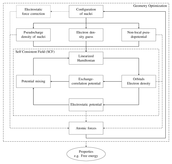
Figure 1: Outline of ground-state DFT simulations in SPARC.

3.1 Finite-difference discretization

The simulations are performed on a cuboidal domain $\Omega$ with boundary $\partial\Omega$ and sides of length $L_{1}$, $L_{2}$ and $L_{3}$. The domain $\Omega$ is discretized using a uniform finite-difference grid with spacing $h$ such that $L_{1}=n_{1}h$, $L_{2}=n_{2}h$ and $L_{3}=n_{3}h$, where $n_{1},n_{2},n_{3}\in\mathbb{N}$, $\mathbb{N}$ being the set of all natural numbers. Each node in the finite-difference grid is indexed by $(i,j,k)$, where $i=1,2,\ldots,n_{1}$, $j=1,2,\ldots,n_{2}$ and $k=1,2,\ldots,n_{3}$. We approximate the Laplacian of any function $f$ at the grid point $(i,j,k)$ using finite-differences:

$$\nabla^{2}_{h}f\big{|}^{(i,j,k)}\approx\sum_{p=0}^{n_{o}}w_{p}\bigg{(}f^{(i+p,j,k)}+f^{(i-p,j,k)}+f^{(i,j+p,k)}+f^{(i,j-p,k)}+f^{(i,j,k+p)}+f^{(i,j,k-p)}\bigg{)}\,,$$ (18)

where $f^{(i,j,k)}$ represents the value of the function $f$ at the node $(i,j,k)$. The weights $w_{p}$ are given by [80, 81]

$$w_{0} = -\frac{1}{h^{2}}\sum_{q=1}^{n_{o}}\frac{1}{q^{2}}\,,$$

$$w_{p} = \frac{2(-1)^{p+1}}{h^{2}p^{2}}\frac{(n_{o}!)^{2}}{(n_{o}-p)!(n_{o}+p)!}\,,\,\,p=1,2,\ldots,n_{o}.$$ (19)

Similarly, we approximate the gradient using the finite-difference approximation:

$$\nabla_{h}f\big{|}^{(i,j,k)}\approx\sum_{p=1}^{n_{o}}\tilde{w}_{p}\bigg{(}(f^{(i+p,j,k)}-f^{(i-p,j,k)})\hat{\mathbf{e}}_{1}+(f^{(i,j+p,k)}-f^{(i,j-p,k)})\hat{\mathbf{e}}_{2}+(f^{(i,j,k+p)}-f^{(i,j,k-p)})\hat{\mathbf{e}}_{3}\bigg{)}\,,$$ (20)

where $\hat{\mathbf{e}}_{1}$, $\hat{\mathbf{e}}_{2}$ and $\hat{\mathbf{e}}_{3}$ signify unit vectors along the edges of $\Omega$, and the weights [80, 81]

$$\tilde{w}_{p}=\frac{(-1)^{p+1}}{hp}\frac{(n_{o}!)^{2}}{(n_{o}-p)!(n_{o}+p)!}\,,\,\,p=1,2,\ldots,n_{o}.$$ (21)

These finite-difference expressions for the Laplacian and gradient represent $\mathcal{O}(h^{2n_{o}})$ accurate approximations. We enforce zero Dirichlet boundary conditions by setting $f^{(i,j,k)}=0$ for any index that does not correspond to a node in the finite-difference grid. While performing spatial integrations, we assume that the function $f$ is constant in a cube of side $h$ around each grid point, i.e.,

$$\int_{\Omega}f({\mathbf{x}})\,\mathrm{d{\mathbf{x}}}\approx h^{3}\sum_{i=1}^{n_{1}}\sum_{j=1}^{n_{2}}\sum_{k=1}^{n_{3}}f^{(i,j,k)}.$$ (22)

Using this integration rule, we approximate the non-local pseudopotential operator as

$$V_{nl}f\big{|}^{(i,j,k)}=\sum_{J=1}^{N}V_{nl,J}f\big{|}^{(i,j,k)}\approx h^{3}\sum_{J=1}^{N}\sum_{lm}\sum_{p=1}^{n_{1}}\sum_{q=1}^{n_{2}}\sum_{r=1}^{n_{3}}\gamma_{Jl}\chi_{Jlm}^{(i,j,k)}\chi_{Jlm}^{(p,q,r)}f^{(p,q,r)}\,.$$ (23)

Henceforth, we denote the Hamiltonian matrix resulting from the above discretization by $\mathbf{H}\in{\mathbb{R}}^{N_{d}\times N_{d}}$, where $N_{d}=n_{1}\times n_{2}\times n_{3}$ is the total number of finite-difference nodes used to discretize $\Omega$. In addition, we represent the eigenvalues of $\mathbf{H}$ arranged in ascending order by $\lambda_{1},\lambda_{2},\ldots,\lambda_{N_{d}}$. We store the discrete Laplacian in compressed row format, apply the nonlocal pseudopotential in a matrix-free way, and store the discrete orbitals as the columns of the dense matrix ${\bf\Psi}\in{\mathbb{R}}^{N_{d}\times N_{s}}$. During parallel computations, we partition the domain as $\Omega=\bigcup\limits_{p=1}^{n_{p}}\Omega_{p}$, where $\Omega_{p}$ denotes the domain local to the $p^{th}$ processor, and $n_{p}$ is the total number of processors. The specific choice of $\Omega_{p}$ corresponds to the PETSc default for structured grids.

3.2 Pseudocharge density generation and self energy calculation

In each step of geometry optimization, the pseudocharge densities are assigned to the grid using the finite-difference approximated Laplacian [26, 68]:

$$b^{(i,j,k)}=\sum_{J=1}^{N}b_{J}^{(i,j,k)}\,,\quad b_{J}^{(i,j,k)}=-\frac{1}{4\pi}\nabla^{2}_{h}V_{J}\big{|}^{(i,j,k)}\,.$$ (24)

The associated discrete self energy is of the form

$$E_{self}^{h}=\frac{1}{2}h^{3}\sum_{J=1}^{N}\sum_{i=1}^{n_{1}}\sum_{j=1}^{n_{2}}\sum_{k=1}^{n_{3}}b_{J}^{(i,j,k)}V_{J}^{(i,j,k)}\,.$$ (25)

Since each radially symmetric pseudopotential $V_{J}$ matches the Coulomb potential outside some prespecified cutoff radius $r_{J}^{c}$, the continuous pseudocharge density $b_{J}$ has compact support in a sphere of radius $r_{J}^{c}$ centered at ${\mathbf{R}}_{J}$. This is not the case for the corresponding discrete pseudocharge density $b_{J}^{(i,j,k)}$, which actually has infinite extent due to the use of the finite-difference Laplacian (Eqn. 24). However, $b_{J}^{(i,j,k)}$ has exponential decay away from $\mathbf{R}_{J}$ (Appendix C), which allows for truncation at some suitably chosen radius $r_{J}^{b}$. It is worth noting that even though the discrete pseudocharge densities may overlap, as long as there is no overlap between the continuous pseudocharge densities, the electrostatic correction to the energy and forces (i.e., $E_{c}$ and $\mathbf{f}_{J,c}$) both rapidly converge to zero as the mesh is refined. This is a consequence of the finite-difference Laplacian being used to assign the pseudocharge densities on to the mesh, with the corresponding inverse operation being performed during the solution of the Poisson equation in Eqn. 14. It is also worth noting that even though the pseudopotential $V_{J}$ might not be smooth—particularly at the cutoff radius $r_{J}^{c}$—we employ a higher-order finite-differences for generating the pseudocharges (Eqn. 24), since they result in smaller values of $r_{J}^{b}$ ($>r_{J}^{c}$), i.e., decay of $b_{J}$ is faster due to a better approximation of the Laplacian.

We calculate the total pseudocharge density $b^{(i,j,k)}$ and the corresponding self energy $E_{self}^{h}$ using the approach outlined in Algorithm 1. We use $P_{r_{J}^{b}}^{p}$ to denote the set of all atoms whose $\Omega_{r_{J}^{b}}$—cube with side of length $2r_{J}^{b}$ centered on the $J^{th}$ atom—has overlap with the processor domain $\Omega_{p}$. We have chosen a cube rather than a sphere due to its simplicity and efficiency within the Euclidean finite-difference discretization. The value of $r_{J}^{b}$ for every type of atom—determined at the start of the complete DFT simulation—is chosen such that the charge constraint in Eqn. 12 is satisfied to within a prespecified normalized tolerance $\varepsilon_{b}$, i.e.,

$$\left|\frac{h^{3}\sum_{i=1}^{n_{1}}\sum_{j=1}^{n_{2}}\sum_{k=1}^{n_{3}}b_{J}^{(i,j,k)}-Z_{J}}{Z_{J}}\right|<\varepsilon_{b}\,.$$ (26)

While describing Algorithm 1, we use the subscripts $s$ and $e$ to denote the starting and ending indices of $\Omega_{r_{J}^{b}}\cap\Omega_{p}\neq\emptyset$, respectively. In this overlap region (and an additional $2n_{0}$ points in each direction), we interpolate $V_{J}^{(i,j,k)}$ on to the finite-difference grid using cubic-splines [82]. Next, we utilize Eqns. 24 and 25 to compute $b^{(i,j,k)}$ and $E_{self}^{h,p}$, where $E_{self}^{h,p}$ is the contribution of the $p^{th}$ processor to the self energy. Finally, we sum the contributions from all the processors to obtain the total self energy $E_{self}^{h}$.

The local and independent nature of the aforedescribed computations ensure that they possess good weak and strong parallel scalability. In addition, they scale as $\mathcal{O}(N)$ with respect to the number of atoms, which makes them efficient even for large systems. In order to achieve perfect $\mathcal{O}(N)$ scaling in practice, the atoms need to be suitably distributed amongst the processors in $\mathcal{O}(N)$ time, after which each processor is only required to go over the local subset of atoms. However, we determine $P_{r_{J}^{b}}^{p}$ by going over all the atoms, which makes the overall procedure formally slightly worse than $\mathcal{O}(N)$ with respect to the number of atoms. Since the system sizes studied in ab-initio calculations are relatively modest, the extra computation in the adopted procedure is negligible.

Input: ${\mathbf{R}}$, $V_{J}$, and $r_{J}^{b}$

$b^{(i,j,k)}=0$, $E_{self}^{h,p}=0$

for $J\in P_{r_{J}^{b}}^{p}$ do

       Determine starting and ending indices $i_{s}$, $i_{e}$, $j_{s}$, $j_{e}$, $k_{s}$, $k_{e}$ for $\Omega_{r^{b}_{J}}\cap\Omega_{p}$

       Determine $V_{J}^{(i,j,k)}$ $\forall$ $i\in[i_{s}-n_{o},i_{e}+n_{o}]$, $j\in[j_{s}-n_{o},j_{e}+n_{o}]$, $k\in[k_{s}-n_{o},k_{e}+n_{o}]$

       $b^{(i,j,k)}_{J}=-\frac{1}{4\pi}\nabla^{2}_{h}V_{J}\big{|}^{(i,j,k)}$,  $b^{(i,j,k)}=b^{(i,j,k)}+b^{(i,j,k)}_{J}$ $\forall$ $i\in[i_{s},i_{e}]$, $j\in[j_{s},j_{e}]$, $k\in[k_{s},k_{e}]$

       $E_{self}^{h,p}=E_{self}^{h,p}+\frac{1}{2}h^{3}b^{(i,j,k)}_{J}V_{J}^{(i,j,k)}$ $\forall$ $i\in[i_{s},i_{e}]$, $j\in[j_{s},j_{e}]$, $k\in[k_{s},k_{e}]$

      

$E_{self}^{h}=\sum_{p=1}^{n_{p}}E_{self}^{h,p}$

Output: $b^{(i,j,k)}$ and $E_{self}^{h}$

Algorithm 1 Pseudocharge density generation and self energy calculation

3.3 Electrostatic potential calculation

The electrostatic potential $\phi$—solution to the Poisson problem in Eqn. 14 on all of space ${\mathbb{R}}^{3}$—needs to be computed in each SCF iteration as part of the linearized Hamiltonian $\mathbf{H}$ . However, since all calculations are restricted to $\Omega$, appropriate boundary conditions need to be prescribed on $\partial\Omega$ in order to minimize the finite-domain effect. Indeed, the simplest choice of zero Dirichlet boundary conditions can result in very slow convergence with domain size, as is evident from the discussion that follows. The electrostatic potential can be written in integral form using the Green’s function of the Laplacian:

$$\phi({\mathbf{x}})=\int_{{\mathbb{R}}^{3}}\frac{\rho({\mathbf{x}}^{\prime})+b({\mathbf{x}}^{\prime},{\mathbf{R}})}{|{\mathbf{x}}-{\mathbf{x}}^{\prime}|}\,{\rm d{\mathbf{x}}^{\prime}}\approx\int_{\Omega}\frac{\rho({\mathbf{x}}^{\prime})+b({\mathbf{x}}^{\prime},{\mathbf{R}})}{|{\mathbf{x}}-{\mathbf{x}}^{\prime}|}\,\rm{d{\mathbf{x}}^{\prime}}\,,$$ (27)

where the exponential decay of the electron density $\rho$ and total pseudocharge $b$ has been used to restrict the integral to $\Omega$. On performing a multipole expansion of the kernel $1/|{\mathbf{x}}-{\mathbf{x}}^{\prime}|$, we arrive at

$$\phi({\mathbf{x}})=\sum_{l=0}^{\infty}\sum_{m=-l}^{l}\frac{4\pi}{(2l+1)|{\mathbf{x}}|^{l+1}}Y_{lm}\left(\frac{{\mathbf{x}}}{|{\mathbf{x}}|}\right)\int_{\Omega}|{\mathbf{x}}^{\prime}|^{l}Y_{lm}\left(\frac{{\mathbf{x}}^{\prime}}{|{\mathbf{x}}^{\prime}|}\right)(\rho({\mathbf{x}}^{\prime})+b({\mathbf{x}}^{\prime}))\rm{d{\mathbf{x}}^{\prime}}\,\,,$$ (28)

where $Y_{lm}$ are the real spherical harmonics. It can therefore be deduced that unlike $\rho$ and $b$, in general $\phi$ only has algebraic decay away from the cluster. Therefore, significant errors can result when zero Dirichlet boundary conditions are employed, particularly for systems with net charge and/or dipole moment. In order to mitigate this, we adopt the procedure described below. We write the discrete form of the Poisson problem in Eqn. 14 as

$$-\frac{1}{4\pi}\nabla_{h}^{2}\phi\big{|}^{(i,j,k)}=\rho^{(i,j,k)}+b^{(i,j,k)}-d^{(i,j,k)}\,,$$ (29)

where zero Dirichlet boundary conditions are prescribed on $\partial\Omega$, and the ‘charge correction’ [83]

$$d^{(i,j,k)} = \frac{-1}{4\pi}\sum_{p=0}^{n_{o}}w_{p}\bigg{(}\chi^{(i+p,j,k)}\phi^{(i+p,j,k)}+\chi^{(i-p,j,k)}\phi^{(i-p,j,k)}+\chi^{(i,j+p,k)}\phi^{(i,j+p,k)}+\chi^{(i,j-p,k)}\phi^{(i,j-p,k)}$$ (30)

$$+ \chi^{(i,j,k+p)}\phi^{(i,j,k+p)}+\chi^{(i,j,k-p)}\phi^{(i,j,k-p)}\bigg{)}\,.$$

In the above expression, $w_{p}$ are the finite-difference weights given by Eqn. 19, and $\chi$ is the indicator function that takes values of $0$ and $1$ when the index does and does not belong to the finite-difference grid, respectively. The values of $\phi^{(i,j,k)}$ corresponding to $\chi^{(i,j,k)}=1$ are calculated using the discrete truncated version of the multipole expansion in Eqn. 28:

$$\phi^{(i,j,k)}=\sum_{l=0}^{l_{max}}\sum_{m=-l}^{l}\frac{4\pi}{(2l+1)|{\mathbf{x}}^{(i,j,k)}|^{l+1}}Y_{lm}^{(i,j,k)}Q_{lm}^{h}\,,$$ (31)

where $l_{max}$ is the maximum angular momentum component, and the discrete multipole moments

$$Q_{lm}^{h}=h^{3}\sum_{r=1}^{n_{1}}\sum_{s=1}^{n_{2}}\sum_{t=1}^{n_{3}}|{\mathbf{x}}^{(r,s,t)}|^{l}Y_{lm}^{(r,s,t)}(\rho^{(r,s,t)}+b^{(r,s,t)})\,.$$ (32)

It is worth noting that the evaluation of $Q_{lm}$ is independent of the position at which the electrostatic potential needs to be evaluated. Therefore, the cost of calculating the charge correction is $\mathcal{O}(N_{d})+\mathcal{O}(N_{d}^{2/3})$, which makes its scaling $\mathcal{O}(N)$ with respect to the number of atoms. The associated prefactors are insignificant since $l_{max}$ is typically very small, and $d^{(i,j,k)}$ only needs to be computed for grid points which lie within a distance of $(n_{o}-1)h$ from the boundary $\partial\Omega$. Therefore, the electrostatic potential $\phi$ can be determined in $\mathcal{O}(N)$ time when sophisticated preconditioners like multigrid [84] are employed for solving the linear system in Eqn. 29. The above strategy is expected to minimize the finite-domain effect resulting from the slow decay of the electrostatic potential, which is indeed verified by the results presented in Section 4.

3.4 Electron density calculation

In each iteration of the SCF method, the electron density corresponding to the linearized Hamiltonian $\mathbf{H}$ needs to be evaluated. This is typically the most computationally expensive step in DFT calculations. In this work, we utilize the Chebyshev filtered subspace iteration (CheFSI) [62, 63] to compute approximations to the lowest $N_{s}$ eigenvalues and corresponding eigenvectors of $\mathbf{H}$. This choice of eigensolver is motivated by the minimal orthogonalization and computer memory costs compared to other eigensolvers commonly employed in electronic structure calculations, e.g. Locally Optimal Block Preconditioned Conjugate Gradient (LOBPCG) [85]. Moreover, the lack of efficient real-space preconditioners limits the effectiveness of diagonalization approaches like LOBPCG in the current setting. In fact, CheFSI has been found to outperform LOBPCG for large scale computations even in the context of plane-waves [86].

The CheFSI algorithm as implemented in SPARC consists of three main steps. First, we filter the guess orbitals $\bf\Psi$ using Chebyshev polynomials:

$${\bf{\Psi}_{f}}=p_{m}({\bf{H}}){\bf\Psi}\,,\quad p_{m}(t)=C_{m}\left(\frac{t-c}{e}\right)\,,$$ (33)

where ${\bf{\Psi}_{f}}$ represents the collection of filtered orbitals, and $C_{m}$ denotes the Chebyshev polynomial of degree $m$. In addition, $e=(\lambda_{N_{d}}-\lambda_{c})/2$ and $c=(\lambda_{N_{d}}+\lambda_{c})/2$, where $\lambda_{c}$ signifies the cutoff chosen for the Chebyshev polynomial filter. The central idea of this technique is to use the rapid growth of Chebyshev polynomials outside the interval $[-1,1]$ to dampen all the eigencomponents corresponding to eigenvalues larger than $\lambda_{c}$. The matrix $p_{m}({\bf{H}})$ is not explicitly determined, rather its product with $\mathbf{\Psi}$ is computed using the three term recurrence relation of Chebyshev polynomials, as outlined in Algorithm 2.

Input: $\bf{H}$, ${\bf{\Psi}}$, $m$, $\lambda_{1}$, $\lambda_{N_{d}}$, $\lambda_{c}$

$e=\frac{\lambda_{N_{d}}-\lambda_{c}}{2}$; $c=\frac{\lambda_{N_{d}}+\lambda_{c}}{2}$; $\sigma=\frac{e}{\lambda_{1}-c}$

${\bf{\Psi}_{f}}=\frac{\sigma}{e}\left({\bf{H}}-c{\bf{I}}\right){\bf{\Psi}}$

for $j=2:m$ do

       ${\bf{\tilde{\Psi}}_{f}}=\frac{2\sigma}{e}\left({\bf{H}}-c{\bf{I}}\right){\bf{\Psi}_{f}}-\left(\frac{\sigma^{2}}{2-\sigma^{2}}\right){\bf{\Psi}}$

       ${\bf{\Psi}}={\bf{\Psi}_{f}}$;   ${\bf{\Psi}_{f}}={\bf{\tilde{\Psi}}_{f}}$;   $\sigma=\frac{\sigma}{2-\sigma^{2}}$

      

Output: ${\bf{\Psi}_{f}}$

Algorithm 2 Chebyshev filtering

Next, we project onto the filtered basis $\mathbf{\Psi_{f}}$ to arrive at the generalized eigenproblem:

$${\mathbf{H_{s}}}\mathbf{y_{n}}=\lambda_{n}\mathbf{M_{s}}\mathbf{y_{n}}\,,\quad n=1,2,\ldots N_{s}\,,$$ (34)

whose eigenvalues represent approximations to those of the Hamiltonian $\mathbf{H}$. The dense matrices $\mathbf{H_{s}},\mathbf{M_{s}}\in{\mathbb{R}}^{N_{s}\times N_{s}}$ are obtained using the relations

$$\mathbf{H_{s}}=\mathbf{\Psi_{f}^{T}}\mathbf{H}\mathbf{\Psi_{f}}\,,\quad\mathbf{M_{s}}=\mathbf{\Psi_{f}^{T}}\mathbf{\Psi_{f}}\,.$$ (35)

After solving the eigenproblem in Eqn. 34, we calculate the Fermi energy $\lambda_{f}$ by enforcing the constraint on the total number of electrons:

$$2\sum_{n=1}^{N_{s}}g_{n}=N_{e}\,,\quad\text{where}\quad g_{n}=\left(1+\exp\left(\frac{\lambda_{n}-\lambda_{f}}{k_{B}T}\right)\right)^{-1}\,.$$ (36)

Finally, we perform the subspace rotation

$$\mathbf{\Psi}=\mathbf{\Psi_{f}}\mathbf{Y}\,,$$ (37)

where the columns of the matrix $\mathbf{Y}\in{\mathbb{R}}^{N_{s}\times N_{s}}$ contain the eigenvectors $\mathbf{y_{n}}$. The columns of $\mathbf{\Psi}$ so obtained represent approximations to the eigenvectors of $\mathbf{H}$, which are then used to calculate the electron density at the finite-difference grid points:

$$\rho^{(i,j,k)}=\frac{2}{h^{3}}\displaystyle\sum_{n=1}^{N_{s}}\,g_{n}\,\psi_{n}^{2(i,j,k)}\,,$$ (38)

where $\psi_{n}^{(i,j,k)}$ are extracted from the $n^{th}$ column of $\mathbf{\Psi}$.

In the very first SCF iteration of the complete DFT simulation, we start with a randomly generated $\mathbf{\Psi}$, and repeat the steps in CheFSI—without calculating/updating the electron density—multiple times ($\sim 3$) [87]. This allows us to obtain a good approximation of the electron density for the second SCF iteration. In principle, this can be achieved by performing the CheFSI steps only once but with a higher degree Chebyshev polynomial $m$. However, in practice this causes the orbitals to become linearly dependent, which is prevented in the current procedure by the orthogonalization step within CheFSI. In every subsequent SCF iteration, we perform the CheFSI steps only once with the subspace rotated $\bf\Psi$ from the previous step as the initial guess. Overall, the calculation of the electron density scales as $\mathcal{O}(N_{s}N_{d})+\mathcal{O}(N_{s}^{2}N_{d})+\mathcal{O}(N_{s}^{3})$, which makes it $\mathcal{O}(N^{3})$ with respect to the number of atoms.

3.5 Free energy calculation

We approximate the integrals in Eqn. 16 using the integration rule in Eqn. 22 to arrive at the following expression for the discrete free energy:

$$\mathcal{\hat{F}}^{h} = 2\sum_{n=1}^{N_{s}}g_{n}\lambda_{n}+h^{3}\sum_{i=1}^{n_{1}}\sum_{j=1}^{n_{2}}\sum_{k=1}^{n_{3}}\bigg{(}\varepsilon_{xc}^{(i,j,k)}\rho^{(i,j,k)}-V_{xc}^{(i,j,k)}\rho^{(i,j,k)}+\frac{1}{2}(b^{(i,j,k)}-\rho^{(i,j,k)})\phi^{(i,j,k)}\bigg{)}$$ (39)

$$-E_{self}^{h}+E_{c}^{h}+2k_{B}T\sum_{n=1}^{N_{s}}\left(g_{n}\log g_{n}+(1-g_{n})\log(1-g_{n})\right)\,,$$

where $E_{self}^{h}$ is the discrete self energy of the pseudocharges (Eqn. 25), and $E_{c}^{h}$ is the discrete repulsive energy correction due to overlapping pseudocharges (Eqn. 48). The evaluation of $\mathcal{\hat{F}}^{h}$ scales as $\mathcal{O}(N_{d})$, and therefore $\mathcal{O}(N)$ with respect to the number of atoms. Even though the free energy needs to be calculated only after the electronic/structural ground-state is determined, it is computed during each step of the SCF method, as is common practice in electronic structure calculations.

3.6 Atomic forces calculation

The discrete form of the atomic force presented in Eqn. 3 is the sum of three components:

$$\mathbf{f}_{J}^{h}=\mathbf{f}_{J,loc}^{h}+\mathbf{f}_{J,c}^{h}+\mathbf{f}_{J,nloc}^{h}\,,$$ (40)

where $\mathbf{f}_{J,loc}^{h}$ is the discrete local component of the force, $\mathbf{f}_{J,c}^{h}$ is the discrete electrostatic correction for overlapping pseudocharges, and $\mathbf{f}_{J,nloc}^{h}$ is the discrete non-local component of the force. Below, we present expressions for $\mathbf{f}_{J,loc}^{h}$ and $\mathbf{f}_{J,nloc}^{h}$, and discuss their evaluation in SPARC. The expression for $\mathbf{f}_{J,c}^{h}$ can be found in Eqn. 50, and its evaluation progresses along similar lines as $\mathbf{f}_{J,loc}^{h}$.

Local component

The local component of the atomic force in discrete form can be written as

$$\mathbf{f}_{J,loc}^{h}=h^{3}\sum_{i=1}^{n_{1}}\sum_{j=1}^{n_{2}}\sum_{k=1}^{n_{3}}\mathbf{\nabla}_{h}b_{J}\big{|}^{(i,j,k)}(\phi^{(i,j,k)}-V_{J}^{(i,j,k)})\,,$$ (41)

where the integral in Eqn. 3 has been approximated using the integration rule in Eqn. 22. The calculation of $\mathbf{f}_{J,loc}^{h}$ proceeds as outlined in Algorithm 3. Specifically, $V_{J}^{(i,j,k)}$ is interpolated on to the finite-difference grid in the overlap region $\Omega_{r_{J}^{b}}\cap\Omega_{p}\neq\emptyset$ (and an additional $4n_{0}$ points in each direction) using cubic-splines, from which $b_{J}^{(i,j,k)}$ is calculated using Eqn. 24. Subsequently, $\mathbf{f}_{J,loc}^{h,p}$—contribution of the $p^{th}$ processor to the local component of the force—is calculated using Eqn. 41. Finally, the contributions from all processors are summed to simultaneously obtain $\mathbf{f}_{J,loc}^{h}$ for all the atoms.

Input: ${\mathbf{R}}$, $\phi^{(i,j,k)}$, $V_{J}$, and $r_{J}^{b}$

for $J\in P_{r_{J}^{b}}^{p}$ do

       Determine starting and ending indices $i_{s}$, $i_{e}$, $j_{s}$, $j_{e}$, $k_{s}$, $k_{e}$ for $\Omega_{r_{J}^{b}}\cap\Omega_{p}$

       Determine $V_{J}^{(i,j,k)}$ $\forall$ $i\in[i_{s}-2n_{o},i_{e}+2n_{o}]$, $j\in[j_{s}-2n_{o},j_{e}+2n_{o}]$, $k\in[k_{s}-2n_{o},k_{e}+2n_{o}]$

       $b_{J}^{(i,j,k)}=-\frac{1}{4\pi}\nabla^{2}_{h}V_{J}\big{|}^{(i,j,k)}$ $\forall$ $i\in[i_{s}-n_{o},i_{e}+n_{o}]$, $j\in[j_{s}-n_{o},j_{e}+n_{o}]$, $k\in[k_{s}-n_{o},k_{e}+n_{o}]$

       $\mathbf{f}_{J,loc}^{h,p}=h^{3}\sum_{i=i_{s}}^{i_{e}}\sum_{j=j_{s}}^{j_{e}}\sum_{k=k_{s}}^{k_{e}}\nabla_{h}b_{J}\big{|}^{(i,j,k)}(\phi^{(i,j,k)}-V_{J}^{(i,j,k)})$

      

$\mathbf{f}_{J,loc}^{h}=\sum_{p=1}^{n_{p}}\mathbf{f}_{J,loc}^{h,p}$

Output: $\mathbf{f}_{J,loc}^{h}$

Algorithm 3 Calculation of the local component of the atomic force.

Non-local component

The non-local component of the force in discrete form can be written as

$$\mathbf{f}_{J,nloc}^{h}=-4\sum_{n=1}^{N_{s}}g_{n}\sum_{lm}\gamma_{Jl}Y_{Jnlm}\mathbf{W}_{Jnlm}\,.$$ (42)

where

$$Y_{Jnlm}=h^{3}\sum_{i=1}^{n_{1}}\sum_{j=1}^{n_{2}}\sum_{k=1}^{n_{3}}\psi_{n}^{(i,j,k)}\chi_{Jlm}^{(i,j,k)}\,,\quad\mathbf{W}_{Jnlm}=h^{3}\sum_{i=1}^{n_{1}}\sum_{j=1}^{n_{2}}\sum_{k=1}^{n_{3}}\nabla_{h}\psi_{n}\big{|}^{(i,j,k)}\chi_{Jlm}^{(i,j,k)}\,\,.$$ (43)

Again, the integral in Eqn. 3 has been approximated using the integration rule in Eqn. 22. The calculation of $\mathbf{f}_{J,nloc}^{h}$ in SPARC is summarized in Algorithm 4. We use $P_{r_{J}^{c}}^{p}$ to denote the set of all atoms whose $\Omega_{r_{J}^{c}}$—cube with side of length $2r_{J}^{c}$ centered on the $J^{th}$ atom—has overlap with the processor domain $\Omega_{p}$. The value of $r_{J}^{c}$ corresponds to the maximum cutoff radius amongst the non-local components of the pseudopotential for the $J^{th}$ atom. We have chosen a cube rather than a sphere due to its simplicity and efficiency within the Euclidean finite-difference discretization. While describing Algorithm 4, we use the subscripts $s$ and $e$ to denote the starting and ending indices of $\Omega_{r_{J}^{c}}\cap\Omega_{p}\neq\emptyset$, respectively. In this overlap region, we interpolate the radial components of the projectors $\chi_{Jlm}^{(i,j,k)}$ on to the finite-difference grid using cubic-splines. Next, we utilize Eqn. 43 to determine $Y_{Jnlm}^{p}$ and $\mathbf{W}_{Jnlm}^{p}$, which represent the contributions of the $p^{th}$ processor to $Y_{Jnlm}$ and $\mathbf{W}_{Jnlm}$, respectively. Finally, we sum the contributions from all the processors to obtain $Y_{Jnlm}$ and $\mathbf{W}_{Jnlm}$, which are then used to calculate $\mathbf{f}_{J,nloc}^{h}$ using Eqn. 42. Overall, the calculation of the atomic forces scales as $\mathcal{O}(N)$ with respect to the number of atoms.

Input: ${\mathbf{R}}$, $\psi_{n}^{(i,j,k)}$, $\gamma_{Jl}$, $\chi_{Jlm}$, and $r_{J}^{c}$

$Y_{Jnlm}^{p}=0$, $\mathbf{W}_{Jnlm}^{p}=0$

for $J\in P_{r_{J}^{c}}^{p}$ do

       Determine starting and ending indices $i_{s}$, $i_{e}$, $j_{s}$, $j_{e}$, $k_{s}$, $k_{e}$ for $\Omega_{r_{J}^{c}}\cap\Omega_{p}$

       Determine $\chi_{Jlm}^{(i,j,k)}$ $\forall$ $i\in[i_{s},i_{e}]$, $j\in[j_{s},j_{e}]$, $k\in[k_{s},k_{e}]$

       $Y_{Jnlm}^{p}=Y_{Jnlm}^{p}+h^{3}\psi_{n}^{(i,j,k)}\chi_{Jlm}^{(i,j,k)}$ $\forall$ $i\in[i_{s},i_{e}]$, $j\in[j_{s},j_{e}]$, $k\in[k_{s},k_{e}]$

       $\mathbf{W}_{Jnlm}^{p}=\mathbf{W}_{Jnlm}^{p}+h^{3}\nabla_{h}\psi_{n}\big{|}^{(i,j,k)}\chi_{Jlm}^{(i,j,k)}$ $\forall$ $i\in[i_{s},i_{e}]$, $j\in[j_{s},j_{e}]$, $k\in[k_{s},k_{e}]$

      

$Y_{Jnlm}=\sum_{p=1}^{n_{p}}Y_{Jnlm}^{p}$, $\mathbf{W}_{Jnlm}=\sum_{p=1}^{n_{p}}\mathbf{W}_{Jnlm}^{p}$

$\mathbf{f}_{J,nloc}^{h}=-4\sum_{n=1}^{N_{s}}g_{n}\sum_{lm}\gamma_{Jl}Y_{Jnlm}\mathbf{W}_{Jnlm}$

Output: $\mathbf{f}_{J,nloc}^{h}$

Algorithm 4 Calculation of the non-local component of the atomic force

4 Examples and Results

In this section, we verify the proposed finite-difference formulation and parallel implementation of DFT for isolated clusters—first component of SPARC (Simulation Package for Ab-initio Real-space Calculations)—through selected examples. In all the simulations, we utilize a twelfth-order accurate finite-difference discretization ($n_{o}=6$), the Perdew-Wang parametrization [88] of the correlation energy calculated by Ceperley-Alder [89], a smearing of $k_{B}T=1\times 10^{-3}$ Ha, and norm-conserving Troullier-Martins pseudopotentials [90]. The values of cutoff radii for the non-local projectors and the choice of local component of the pseudopotentials are specified in Appendix B.

We truncate the discrete multipole expansion presented in Eqn. 31 at $l_{max}=6$. We solve the linear system in Eqn. 29—discrete form of the Poisson problem in Eqn. 14—using the Conjugate Gradient (CG) method [91] with the block-Jacobi preconditioner [92]. In the CheFSI method, we determine the extremal eigenvalues of the Hamiltonian $\mathbf{H}$ using a few iterations of the Lanczos method [93], set the number of states to be $N_{s}=N_{e}/2+30$, utilize a polynomial of degree $m=20$ for Chebyshev filtering, and choose the filter cutoff $\lambda_{c}$ to be the previous iteration’s Fermi energy plus $0.1$ Ha. Further, we solve the generalized eigenproblem in Eqn. 34 using the QR algorithm [94] as implemented in LAPACK [95]. We calculate the Fermi energy—root of the constraint in Eqn. 36—using Brent’s method [96]. We use Anderson mixing [97] with relaxation parameter of $0.3$ and mixing history of $7$ for accelerating the convergence of the Self-Consistent Field (SCF) method. Finally, we employ the Polak-Ribiere variant of non-linear conjugate gradients with a secant line search [98] for performing geometry optimization.

In all the calculations, the energy and forces are converged to within the ‘chemical accuracy’ of $0.001$ Ha/atom in energy and $0.001$ Ha/Bohr, respectively. Wherever applicable, the results obtained by SPARC are compared to the well established plane-wave code ABINIT [15, 99, 100]. The error in energy is defined as the difference in the magnitude, and the error in forces is defined to be the maximum difference in any component on any atom. The simulations are performed on a computer cluster consisting of $16$ nodes with the following configuration: Altus 1804i Server - 4P Interlagos Node, Quad AMD Opteron 6276, 16C, 2.3 GHz, 128GB, DDR3-1333 ECC, 80GB SSD, MLC, 2.5" HCA, Mellanox ConnectX 2, 1-port QSFP, QDR, memfree, CentOS, Version 5, and connected through InfiniBand cable.

4.1 Convergence with domain size

We first verify the convergence of the computed energy and atomic forces with respect to the size of the domain $\Omega$. We choose the carbon monoxide (CO) and water (H₂O) molecules as representative examples, with the C-O and O-H bond lengths reduced and increased by $8\%$ from their equilibrium values as determined by ABINIT, respectively. The polar nature of the molecules and their deliberate asymmetric positioning within $\Omega$ ensure that any finite-domain effects are exaggerated. In Fig. 2, we present convergence of the energy and atomic forces for $h=0.2$ Bohr as $\{L_{1},L_{2},L_{3}\}$ is increased from $\{12,12,12\}$ Bohr to $\{18,18,18\}$ Bohr, with the results obtained for $\{L_{1},L_{2},L_{3}\}=\{40,40,40\}$ Bohr used as reference. We observe exponential convergence of both the energy and the forces to well below accuracies desired in DFT calculations. In fact, even a domain size of $\{L_{1},L_{2},L_{3}\}=\{12,12,12\}$ is sufficient to obtain chemical accuracy in both energy and forces. The corresponding electron density contours for H₂O are plotted in Fig. 3. Overall, these results demonstrate the efficacy of SPARC’s electrostatic formulation in minimizing the finite-domain effect for isolated clusters.

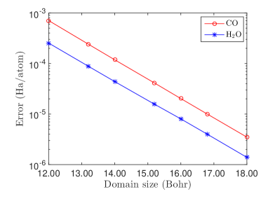
(a) Energy

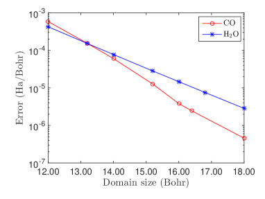
(b) Forces

Figure 2: Convergence of energy and atomic forces with respect to domain size for the CO and H₂O molecules.

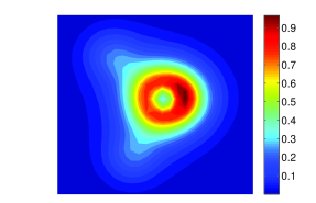
Figure 3: In-plane electron density contours for the H₂O molecule.

4.2 Convergence with spatial discretization

We next verify the convergence of the computed energy and atomic forces with respect to the finite-difference mesh-size. As representative examples, we choose the icosahedral Platinum (Pt₁₃), icosahedral Gold (Au₁₃), and $\beta$-Aminoisobutyric acid tri-TMS II (C₁₃H₃₃NO₂Si₃) clusters with domain sizes of $\{L_{1},L_{2},L_{3}\}=\{36,36,36\}$, $\{40,40,40\}$ and $\{42,38,34\}$ Bohr, respectively. All errors are defined with respect to ABINIT, wherein we employ plane-wave cutoffs of $42$, $42$, and $68$ Ha along with domain sizes of $\{L_{1},L_{2},L_{3}\}=\{42,42,42\}$, $\{42,42,42\}$, and $\{50,46,42\}$ Bohr for Pt₁₃, Au₁₃, and C₁₃H₃₃NO₂Si₃, respectively. The resulting reference energies and forces are converged to within $5.0\times 10^{-6}$ Ha/atom and $5.0\times 10^{-6}$ Ha/Bohr, respectively. In Fig. 4, we plot error in the SPARC energy and forces with respect to the mesh size, from which it is clear that there is systematic convergence of both energies and forces. On performing a fit to the data, we obtain average convergence rates of approximately $\mathcal{O}(h^{9})$ in the energy and $~{}\mathcal{O}(h^{8})$ in the forces. In doing so, the desired accuracy is readily attained. In Fig. 5, we present the computed isosurfaces for Au₁₃ and C₁₃H₃₃NO₂Si₃. Overall, we conclude that SPARC is able to obtain high convergence rates in both the DFT energy and atomic forces, which contributes to its accuracy and efficiency. Moreover, the energy and forces converge at comparable rates, without need of additional measures such as double-grid [101] or high-order integration [59] techniques.

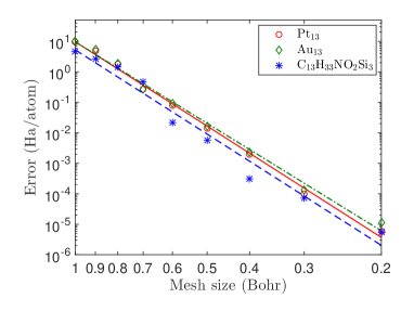
(a) Energy

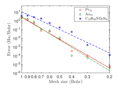
(b) Forces

Figure 4: Convergence of the energy and atomic forces with respect to mesh size to reference planewave result for the Pt₁₃, Au₁₃, and C₁₃H₃₃NO₂Si₃ clusters.

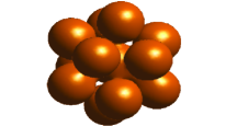
(a) Au₁₃

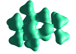
(b) C₁₃H₃₃NO₂Si₃

Figure 5: Electron density isosurface for $\rho=0.05$ Bohr^-3

4.3 Ground state properties

We now verify that the ground-state properties of isolated clusters can be accurately determined using SPARC. For this purpose, we select the Hydrogen (H₂), Nitrogen (N₂), and Oxygen (O₂) molecules, a domain size of $\{L_{1},L_{2},L_{3}\}=\{24,24,24\}$ Bohr, and mesh-size of $h=0.2$ Bohr. We begin by evaluating the energy and force as a function of interatomic distance, the results of which are presented in Fig. 6. Specifically, we plot the energy as a function of bond length along with its cubic spline fit in Fig. 6a, and the computed interatomic force and the derivative of the cubic spline fit to the energy in Fig. 6b. The evident agreement demonstrates that the computed energy and atomic forces are indeed consistent. Moreover, there is no noticeable ‘egg-box’ effect [102]—a phenomenon arising due to the breaking of the translational symmetry—at meshes required for obtaining chemical accuracies.

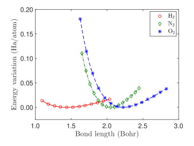
(a) Computed energy and its cubic spline fit

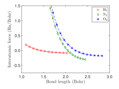
(b) Computed force and the derivative of the cubic spline fit to the energy

Figure 6: Variation in the computed energy and atomic force as a function of interatomic distance for the H₂, N₂, and O₂ molecules.

Next, we use the above results to calculate the vibrational frequency for the H₂, N₂, and O₂ molecules using the relation [103]:

$$\nu=\frac{1}{2\pi c}\left(\frac{k}{\mu}\right)^{\frac{1}{2}}\,,$$ (44)

where $c$ is the speed of light, $k$ is the derivative of the cubic spline fit to the force at the equilibrium bond length, and $\mu$ is the reduced mass of the system. In ABINIT, we choose a domain size of $\{L_{1},L_{2},L_{3}\}=\{30,30,30\}$ Bohr for all three systems and planewave cutoffs of $32$ Ha, $40$ Ha, and $38$ Ha for H₂, N₂, and O₂, respectively. From the results presented in Table 1, we observe that there is excellent agreement between SPARC and ABINIT, with the maximum difference in the vibrational frequency being $8$ $cm^{-1}$. There is also good agreement between DFT and experiment, highlighting the accuracy of DFT as an ab-initio theory. These results further verify that SPARC is able to obtain accurate atomic forces, a critical feature for both structural relaxations and ab-initio molecular dynamics.

Molecule	SPARC	ABINIT	Experiment [104, 105]
H2	$4007$	$4014$	$4401$
N2	$2448$	$2456$	$2358$
O2	$1649$	$1642$	$1580$

Table 1: Vibrational frequency in $cm^{-1}$ for the H₂, N₂, and O₂ molecules.

Finally, we randomly perturb the atomic positions in the three molecules such that the interatomic distance differs by up to $15$ percent from the equilibrium bond length. We maximize generality by ensuring that the resulting systems are not aligned with any of the coordinate axes. In Table 2, we present the results of the geometry optimization by SPARC, and compare them with ABINIT for the aforementioned choice of parameters. We observe that there is very good agreement between SPARC and ABINIT, with the maximum difference in the energy being $0.0007$ Ha/atom, and the maximum difference in the equilibrium bond length being $0.001$ Bohr. These results are also in excellent agreement with the data plotted in Fig. 6. Overall the results indicate that SPARC is able to accurately determine ground state properties for isolated clusters.

Molecule	Energy (Ha/atom)		Bond length (Bohr)
	SPARC	ABINIT	SPARC	ABINIT
H2	$-0.5682$	$-0.5681$	$1.437$	$1.437$
N2	$-9.9463$	$-9.9460$	$2.049$	$2.049$
O2	$-15.8717$	$-15.8710$	$2.226$	$2.227$

Table 2: Ground state energy and equilibrium configuration for the H₂, N₂, and O₂ molecules.

4.4 Scaling and performance

In previous subsections, we have verified the accuracy of SPARC by comparing with the well-established plane-wave code ABINIT. We now investigate the efficiency of SPARC relative to ABINIT, for which we choose bulk-terminated Silicon nanoclusters passivated by Hydrogen as representative examples. In all the calculations, we utilize a mesh-size of $h=0.5$ Bohr in SPARC, and a planewave energy cutoff of $16$ Ha in ABINIT. Further, we employ a vacuum of $5$ Bohr in both SPARC and ABINIT. We choose all the other parameters so as to obtain the chemical accuracy of $0.001$ Ha/atom in the energy and $0.001$ Ha/Bohr in the atomic force. All the times reported here include the calculation of the electronic ground-state as well as the atomic force. The detailed breakdown of the timings for SPARC can be found in the output files provided with the code accompanying this paper.

First, we compare the strong scaling of SPARC with ABINIT for the Si₂₇₅H₁₇₂ cluster. We utilize $2$, $8$, $64$, $128$, $512$, and $640$ cores for performing the simulation using SPARC. We use $6$, $9$, $37$, $296$, $592$, and $666$ cores for ABINIT, which it suggests are optimal in the range of cores considered here. Both SPARC and ABINIT require $19$ iterations for convergence of the SCF method. In Fig. 7a, we present the wall time taken by SPARC and ABINIT as the number of processors is increased. We observe that both SPARC and ABINIT display similar trends with respect to strong scaling. Specifically, the SPARC and ABINIT curves are close to being parallel, with no further reduction in wall time observed after approximately $700$ cores for SPARC and $600$ cores for ABINIT. However, the prefactors are significantly different, with SPARC being able to outperform ABINIT by up to factors of $7$.

Next, we compare the weak scaling of SPARC with ABINIT for the Si₂₉H₃₆, Si₇₁H₈₄, Si₂₇₅H₁₇₂, Si₅₂₅H₂₇₆, and Si₈₄₉H₃₇₂ nanoclusters. The number of electrons in these systems range from $152$ (Si₂₉H₃₆) to $3768$ (Si₈₄₉H₃₇₂). For both SPARC and ABINIT, we fix the number of electrons per core to be approximately $160$, and select at most $4$ cores from every compute node. In Figure 7b, we present the results so obtained for the variation in total CPU time versus the number of electrons. We observe similar scaling for both codes, with $\mathcal{O}(N_{e}^{2.51})$ for SPARC and $\mathcal{O}(N_{e}^{2.75})$ for ABINIT. However, the prefactor for SPARC is again noticeably lower, with speedups over ABINIT ranging from factors of $3$ to $7$.

The superior performance of SPARC relative to ABINIT for the examples considered here merits further consideration. In SPARC, more than $84\%$ of the total time is spent in the Chebyshev filtering, subspace projection, and subspace rotation steps. In ABINIT, more than $90\%$ of the time is spent in the subroutines fourwf (FFTs for the wavefunctions), nonlop (non-local pseudopotential related computations), and projbd (Gram-Schmidt orthogonalizations). Since the number of orthogonalizations in the CheFSI method is very small—particularly when compared to LOBPCG—it is not a significant component in SPARC. Inspite of this, though the implementation of CheFSI in ABINIT is competitive compared to LOBPCG for some systems, it is slower for other systems, due to the lack of preconditioning in CheFSI [86]. Therefore, it appears that the main reason for the speedup of SPARC over ABINIT is that the Hamiltonian operator can be applied more efficiently within the finite-difference discretization.

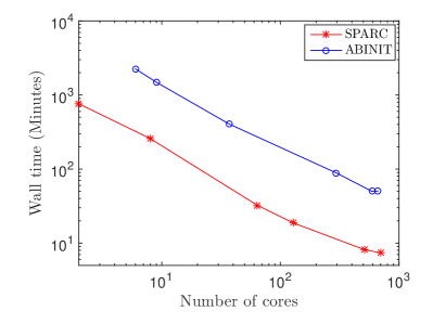
(a) Strong scaling

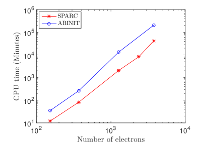
(b) Weak scaling

Figure 7: Strong and weak scaling behavior for hydrogen passivated silicon nanoclusters. The system utilized for strong scaling is Si₂₇₅H₁₇₂. The systems employed for weak scaling are Si₂₉H₃₆, Si₇₁H₈₄, Si₂₇₅H₁₇₂, Si₅₂₅H₂₇₆ and Si₈₄₉H₃₇₂.

Finally, we compare the minimum wall time achievable by SPARC and ABINIT for the aforementioned nanoclusters with the exception of Si₈₄₉H₃₇₂, for which the resources currently available to us are insufficient. While performing this study, we restrict the maximum number of electrons per computational core to $160$. In SPARC, we choose the number of cores as multiples of $64$, whereas we select the number of cores and parallelization scheme in ABINIT as suggested by it. We present the results so obtained in Table 3. We observe that SPARC is able to achieve smaller wall times by factors larger than $6.8$ compared to ABINIT for all the systems considered. In particular, SPARC requires a factor of approximately $7.0$ less wall time than ABINIT for the Si₅₂₅H₂₇₆ nanocluster. Overall, these results indicate that SPARC is a highly efficient DFT formulation and implementation that is highly competitive with well-optimized plane-wave codes.

System	SPARC	ABINIT
Si29H36	$0.69$ $(128)$	$7.30$ $(106)$
Si71H84	$1.15$ $(320)$	$8.10$ $(321)$
Si275H172	$7.39$ $(704)$	$50.60$ $(666)$
Si525H276	$32.45$ $(960)$	$227.56$ $(1008)$

Table 3: Minimum wall time in minutes for hydrogen passivated silicon nanoclusters. The number in brackets represents the number of cores on which the minimum wall time is achieved.

5 Concluding Remarks

In this work, we have developed an accurate and efficient finite-difference formulation and parallel implementation of Density Functional Theory (DFT) for isolated clusters, which represents the first component of SPARC (Simulation Package for Ab-initio Real-space Calculations). Specifically, employing the Chebyshev polynomial filtered self-consistent field iteration in conjunction with the reformulation of the electrostatics and the non-local component of the atomic force, we have developed a framework using the finite-difference representation wherein energies and forces can be efficiently evaluated to within the accuracies desired in electronic structure calculations. Through a variety of examples consisting of both light and heavy elements, we have demonstrated that SPARC obtains exponential convergence in energies and forces with domain size; systematic convergence in the energy and forces with respect to spatial discretization at comparably high rates to reference plane-wave results; forces that are consistent with the energy, both being free from any noticeable ‘egg-box’ effect; and accurate ground-state properties like equilibrium energies, geometries and vibrational spectra. Moreover, we have shown that the weak and strong parallel scaling of SPARC is very similar to well-established and optimized plane-wave codes for systems consisting of up to thousands of electrons, but with a significantly smaller prefactor.

The examples in this work have been restricted to $\sim 1000$ atoms so that we could perform a thorough analysis of the accuracy and efficiency of SPARC within the computational resources routinely available to us. However, larger systems can indeed be studied, e.g., we have performed a simulation for Si₃₁₄₅H₈₇₆ using SPARC. Nevertheless, we note that there is scope for significant improvement in SPARC. Specifically, the subspace eigenvalue problem—currently solved in serial—is expected to become the dominant cost for systems consisting of tens of thousands of electrons. Therefore, incorporating efficient and scalable parallel eigendecomposition techniques into SPARC is currently being undertaken by the authors. These improvements along with optimization of code are expected to further improve the efficiency of SPARC. The extension of SPARC to enable the study of systems with periodicity in one, two, and three directions is also a worthy subject for future work, and is therefore being pursued by the authors.

Appendix

Appendix A Electrostatic correction for overlapping pseudocharge densities

In ab-initio calculations, even if the pseudopotential approximation is employed, the repulsive energy is still calculated with the nuclei treated as point charges. The electrostatic formulation employed in this work does not make this distinction, resulting in disagreement with convention for overlapping pseudocharge densities. The correction to the repulsive energy which reestablishes agreement can be written as [68]

$$E_{c}({\mathbf{R}}) = \frac{1}{2}\int_{{\mathbb{R}}^{3}}\left(\tilde{b}({\mathbf{x}},{\mathbf{R}})+b({\mathbf{x}},{\mathbf{R}})\right)V_{c}({\mathbf{x}},{\mathbf{R}})\,\mathrm{d{\mathbf{x}}}+\frac{1}{2}\sum_{J=1}^{N}\int_{{\mathbb{R}}^{3}}b_{J}({\mathbf{x}},{\mathbf{R}}_{J})V_{J}({\mathbf{x}},{\mathbf{R}}_{J})\,\mathrm{d{\mathbf{x}}}$$ (45)

$$-\frac{1}{2}\sum_{J=1}^{N}\int_{{\mathbb{R}}^{3}}\tilde{b}_{J}({\mathbf{x}},{\mathbf{R}}_{J})\tilde{V}_{J}({\mathbf{x}},{\mathbf{R}}_{J})\,\mathrm{d{\mathbf{x}}}\,,$$

where

$$V_{c}({\mathbf{x}},{\mathbf{R}})=\sum_{J=1}^{N}\left(\tilde{V}_{J}({\mathbf{x}},{\mathbf{R}}_{J})-V_{J}({\mathbf{x}},{\mathbf{R}}_{J})\right)\,.$$ (46)

In addition, $\tilde{b}$ denotes the reference pseudocharge density, and $\tilde{b}_{J}$ represents the spherically symmetric and compactly supported reference charge density of the $J^{th}$ nucleus that generates the potential $\tilde{V}_{J}$, i.e.,

$$\tilde{b}({\mathbf{x}},{\mathbf{R}})=\sum_{J=1}^{N}\tilde{b}_{J}({\mathbf{x}},{\mathbf{R}}_{J})\,,\quad\tilde{b}_{J}({\mathbf{x}},{\mathbf{R}}_{J})=-\frac{1}{4\pi}\nabla^{2}\tilde{V}_{J}({\mathbf{x}},{\mathbf{R}}_{J})\,,\quad\int_{{\mathbb{R}}^{3}}\tilde{b}_{J}({\mathbf{x}},{\mathbf{R}}_{J})\,\mathrm{d{\mathbf{x}}}=Z_{J}\,.$$ (47)

The discrete form of the repulsive energy correction is obtained by approximating the integrals in Eqn. 45 using the integration rule in Eqn. 22:

$$E_{c}^{h}=\frac{1}{2}h^{3}\sum_{i=1}^{n_{1}}\sum_{j=1}^{n_{2}}\sum_{k=1}^{n_{3}}\left((\tilde{b}^{(i,j,k)}+b^{(i,j,k)})V_{c}^{(i,j,k)}+\sum_{J=1}^{N}b_{J}^{(i,j,k)}V_{J}^{(i,j,k)}-\sum_{J=1}^{N}\tilde{b}_{J}^{(i,j,k)}\tilde{V}_{J}^{(i,j,k)}\right)\,,$$ (48)

where $V_{c}^{(i,j,k)}$ is obtained using Eqn. 46.

The correction in the atomic forces arising from the overlapping pseudocharges can be written as [68]

$$\mathbf{f}_{J,c}({\mathbf{R}}) = \frac{1}{2}\int_{{\mathbb{R}}^{3}}\bigg{[}\nabla\tilde{b}_{J}({\mathbf{x}},{\mathbf{R}}_{J})\left(V_{c}({\mathbf{x}},{\mathbf{R}})-\tilde{V}_{J}({\mathbf{x}},{\mathbf{R}}_{J})\right)+\nabla b_{J}({\mathbf{x}},{\mathbf{R}}_{J})\left(V_{c}({\mathbf{x}},{\mathbf{R}})+V_{J}({\mathbf{x}},{\mathbf{R}}_{J})\right)$$

$$+ \left(\nabla\tilde{V}_{J}({\mathbf{x}},{\mathbf{R}}_{J})-\nabla V_{J}({\mathbf{x}},{\mathbf{R}}_{J})\right)\left(\tilde{b}({\mathbf{x}},{\mathbf{R}})+b({\mathbf{x}},{\mathbf{R}})\right)+b_{J}({\mathbf{x}},{\mathbf{R}}_{J})\nabla V_{J}({\mathbf{x}},{\mathbf{R}}_{J})$$

$$- \tilde{b}_{J}({\mathbf{x}},{\mathbf{R}}_{J})\nabla\tilde{V}_{J}({\mathbf{x}},{\mathbf{R}}_{J})\bigg{]}\,\mathrm{d{\mathbf{x}}}\,,$$

whose discrete form is

$$\mathbf{f}_{J,c}^{h} = \frac{1}{2}h^{3}\sum_{i=1}^{n_{1}}\sum_{j=1}^{n_{2}}\sum_{k=1}^{n_{3}}\bigg{(}\nabla_{h}\tilde{b}\big{|}^{(i,j,k)}\left(V_{c}^{(i,j,k)}-\tilde{V}_{J}^{(i,j,k)}\right)+\nabla_{h}b_{J}\big{|}^{(i,j,k)}\left(V_{c}^{(i,j,k)}+V_{J}^{(i,j,k)}\right)$$ (50)

$$+\nabla_{h}(\tilde{V}_{J}-V_{J})\big{|}^{(i,j,k)}\left(\tilde{b}^{(i,j,k)}+b^{(i,j,k)}\right)+b_{J}^{(i,j,k)}\nabla_{h}V_{J}\big{|}^{(i,j,k)}-\tilde{b}_{J}^{(i,j,k)}\nabla_{h}\tilde{V}_{J}\big{|}^{(i,j,k)}\bigg{)}\,.$$

It is worth noting that an alternative to the above formulation is to correct for the error in the repulsive energy and the corresponding force by only considering the pseudocharges that overlap. However, this requires the creation of neighbor lists, which need to be updated at every relaxation step. In SPARC, we employ the corrections in Eqns. 48 and 50 because of their simplicity and accuracy in the context of our electrostatic formulation, and their efficiency in the setting of scalable high performance computing.

In order to demonstrate the importance of the aforedescribed energy and force corrections, we plot their values as a function of interatomic distance for the N₂ and O₂ molecules ($h=0.2$ Bohr) in Fig. 8. We observe that though the magnitude of the energy and force corrections reduce as the distance between the atoms is increased, they are still significant at the equilibrium bond length. Notably, even at distances of around $2r_{J}^{c}\sim 3$ Bohr (Table 4), the force corrections have magnitude of approximately $0.01$ Ha/Bohr. This is because, even though the Troullier-Martins pseudopotentials have non-local projectors that are identically zero outside $r_{J}^{c}$, each of pseudopotentials individually approach the Coulomb potential at values that are noticeably larger than $r_{J}^{c}$. This highlights the need for incorporating the repulsive energy and corresponding atomic force corrections within SPARC, and possibly other real-space DFT implementations that utilize the reformulation of the electrostatics in terms of the pseudocharges, particularly for structural relaxations and molecular dynamics simulations.

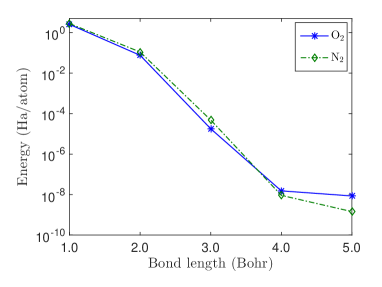
(a) Energy correction

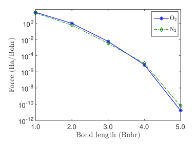
(b) Atomic force correction

Figure 8: Variation in magnitude of the repulsive energy and corresponding atomic force corrections as a function of interatomic distance for the N₂ and O₂ molecules.

Appendix B Pseudopotential parameters

In Table 4, we list the cutoff radii ($r_{J}^{c}$) used for generating the different angular momentum components within the Troullier-Martins pseudopotential. We choose the $l=0$ pseudopotential component as local in all the simulations.

Atom type	Radial cutoff (Bohr)
	$l=0$	$l=1$	$l=2$
H	$1.25$	$-$	$-$
C	$1.50$	$1.54$	$-$
N	$1.50$	$1.50$	$-$
O	$1.45$	$1.45$	$-$
Si	$1.80$	$1.80$	$1.80$
Pt	$2.45$	$2.45$	$2.45$
Au	$2.60$	$2.60$	$2.60$

Table 4: Cutoff radii for non-local projectors within the Troullier-Martins pseudopotential.

Appendix C Properties of the discrete pseudocharge density

The continuous pseudocharge density for the atom positioned at ${\mathbf{R}}_{J}$ has compact support in a sphere of radius $r_{J}^{c}$ centered at ${\mathbf{R}}_{J}$, where $r_{J}^{c}$ is the cutoff radius for the local component of the pseudopotential. Though the corresponding discrete pseudocharge density has infinite extent, it still possesses exponential decay. This is evident from Fig. 9, where we plot the normalized error in the net enclosed charge as a function of the pseudocharge radius $r_{J}^{b}$ for a mesh-size of $h=0.5$ Bohr. It is clear that a suitable finite truncation radius can indeed be chosen such that there is no significant loss of accuracy.

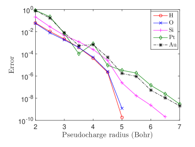
Figure 9: Normalized error in the net enclosed charge as a function of pseudocharge radius. The results for carbon and nitrogen are identical to oxygen.

In this work, we choose the truncation radius $r_{J}^{b}$ for each pseudocharge density such that Eqn. 26 is satisfied to within a tolerance of $\varepsilon_{b}=10^{-8}$. In Fig. 10, we plot the $r_{J}^{b}$ required to achieve this desired accuracy as a function of mesh-size. It is clear that as the mesh becomes finer, $r_{J}^{b}$ becomes smaller, with $r_{J}^{b}\rightarrow r_{J}^{c}$ as $h\rightarrow 0$. The slight non-monotonicity of the curves plotted in Fig. 10 is due to the fact that $r_{J}^{b}$ is chosen to be a multiple of the mesh size $h$ in SPARC.

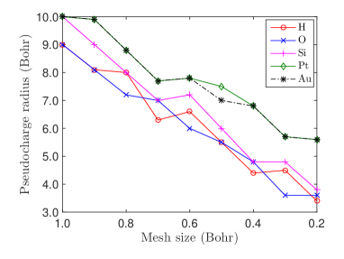
Figure 10: Variation of pseudocharge radius as a function of mesh spacing. The results for carbon and nitrogen are identical to oxygen.

Appendix D Comparison of SPARC with other finite-difference DFT codes

We now study the performance of SPARC relative to PARSEC [34] and OCTOPUS [35], two well-established DFT codes that employ the finite-difference discretization. First, we determine the convergence in energy and atomic forces as a function of mesh-size $h$ for the Si₂₉H₃₆ cluster with the central Silicon atom perturbed by [$0.4$ $0.3$ $0.6$] Bohr. All errors are defined with respect to ABINIT, wherein we employ a plane-wave cutoff of $30$ Ha and domain size of $\{L_{1},L_{2},L_{3}\}=\{42,42,42\}$ Bohr, which results in reference energies and forces that are converged to within $5.0\times 10^{-6}$ Ha/atom and $5.0\times 10^{-6}$ Ha/Bohr, respectively. On performing a fit to the data presented in Fig. 11, we obtain $\mathcal{O}(h^{8.85})$, $\mathcal{O}(h^{7.15})$, and $\mathcal{O}(h^{8.64})$ convergence in energy for SPARC, PARSEC, and OCTOPUS, respectively. Correspondingly, we obtain $\mathcal{O}(h^{9.62})$, $\mathcal{O}(h^{10.05})$, and $\mathcal{O}(h^{10.09})$ convergence in the forces. Though the convergence rates of all three codes are comparable, the associated prefactor in PARSEC is noticeably larger, particularly for the atomic forces.

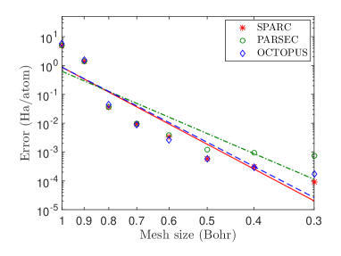
(a) Energy

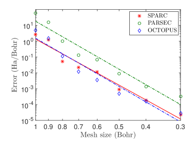
(b) Forces

Figure 11: Convergence of the energy and atomic forces with respect to mesh size to reference planewave result for the Si₂₉H₃₆ cluster.

Next, we perform the strong and weak scaling tests described in Section 4.4 for SPARC, PARSEC, OCTOPUS, and ABINIT. In order to achieve the desired accuracy of $0.001$ Ha/atom in the energy and $0.001$ Ha/Bohr in the atomic forces, we choose a plane-wave cutoff of $16$ Ha in ABINIT, and mesh-sizes of $h=0.5$ Bohr, $h=0.3$ Bohr, and $h=0.5$ Bohr in SPARC, PARSEC, and OCTOPUS, respectively. We also determine the timings for $h=0.5$ Bohr in PARSEC. We present the results so obtained in Fig. 12, wherein the time taken for the first SCF iteration has been excluded. In strong scaling, the minimum wall time achieved by SPARC is smaller by factors of $21$ ($221$ for $h=0.3$ Bohr in PARSEC), $14$, and $6.8$ relative to PARSEC, OCTOPUS, and ABINIT, respectively. In weak scaling, the increase in CPU time with number of electrons for SPARC, PARSEC, OCTOPUS, and ABINIT is $\mathcal{O}(N_{e}^{2.54})$, $\mathcal{O}(N_{e}^{3})$, $\mathcal{O}(N_{e}^{3.19})$, and $\mathcal{O}(N_{e}^{2.75})$, respectively. It is clear that SPARC is able to outperform PARSEC because of the significantly higher efficiency in strong scaling. In OCTOPUS, $>70\%$ (increases with system size) of the time is spent in the function GRAM_SCHMIDT (orthogonalizations), which suggests that CheFSI is significantly superior to Conjugate Gradients (default eigensolver in OCTOPUS) for real-space DFT calculations. Notably, even when RMM-DIIS is employed in OCTOPUS, SPARC demonstrates superior performance. For example, SPARC is faster than OCTOPUS by factors of $3.9$ and $5.76$ for the Si₂₇₅H₁₇₂ and Si₅₂₅H₂₇₆ systems in the weak scaling study, respectively. This is a consequence of the significantly larger number of iterations required by RMM-DIIS in OCTOPUS.

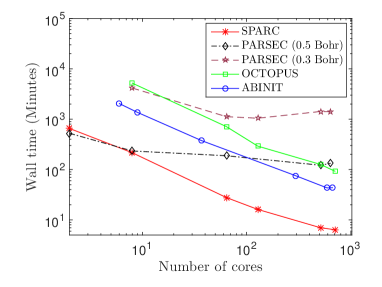
(a) Strong scaling

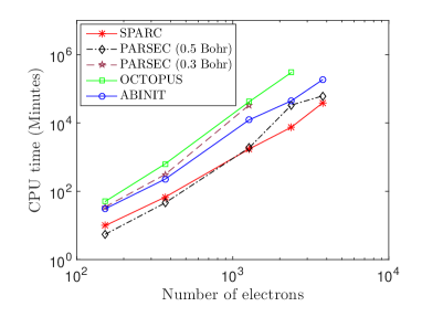
(b) Weak scaling

Figure 12: Strong and weak scaling behavior for hydrogen passivated silicon nanoclusters. The system utilized for strong scaling is Si₂₇₅H₁₇₂. The systems employed for weak scaling are Si₂₉H₃₆, Si₇₁H₈₄, Si₂₇₅H₁₇₂, Si₅₂₅H₂₇₆ and Si₈₄₉H₃₇₂. The time taken for the first SCF iteration has been excluded.

Finally, we compare the minimum wall time—excluding the time for the first SCF iteration—that can be achieved by SPARC, PARSEC, OCTOPUS, and ABINIT for the aforementioned hydrogen passivated nanoclusters. From the results presented in Table 5, we observe that SPARC demonstrates speedup by up to factors of $21$ ($164$ for $h=0.3$ Bohr in PARSEC), $15$, and $7$ compared to PARSEC, OCTOPUS, and ABINIT, respectively. Overall, these results demonstrate that SPARC is an efficient DFT formulation and implementation that is highly competitive with well-established finite-difference and plane-wave codes. In addition, previous finite-difference DFT codes are unable to consistently outperform plane-wave codes in achieving the desired accuracy for the examples considered here.

System	SPARC	PARSEC	PARSEC	OCTOPUS	ABINIT
	$h=0.5$ Bohr	$h=0.5$ Bohr	$h=0.3$ Bohr	$h=0.5$ Bohr	$E_{cut}=16$ Ha
Si29H36	$0.55$ $(128)$	$3.22$ $(8)$	$18.92$ $(16)$	$2.8$ $(256)$	$6.25$ $(106)$
Si71H84	$0.96$ $(320)$	$10.32$ $(64)$	$50.53$ $(64)$	$10.15$ $(512)$	$6.70$ $(321)$
Si275H172	$6.39$ $(704)$	$121.96$ $(512)$	$1046.00$ $(128)$	$92.78$ $(1024)$	$43.76$ $(666)$
Si525H276	$29.00$ $(960)$	$619.72$ $(512)$	—	$366.12$ $(1024)$	$203.30$ $(1008)$

Table 5: Minimum wall time in minutes for hydrogen passivated silicon nanoclusters. The number in brackets represents the number of cores on which the minimum wall time is achieved. The time taken for the first SCF iteration has been excluded.

References

- Hohenberg and Kohn [1964] P. Hohenberg, W. Kohn, Physical Review 136 (1964) B864–B871.
- Kohn and Sham [1965] W. Kohn, L. J. Sham, Physical Review 140 (1965) A1133–A1138.
- Jones and Gunnarsson [1989] R. O. Jones, O. Gunnarsson, Rev. Mod. Phys. 61 (1989) 689–746.
- Ziegler [1991] T. Ziegler, Chemical Reviews 91 (1991) 651–667.
- Kohn et al. [1996] W. Kohn, A. D. Becke, R. G. Parr, The Journal of Physical Chemistry 100 (1996) 12974–12980.
- Jones [2015] R. O. Jones, Rev. Mod. Phys. 87 (2015) 897–923.
- Parr and Yang [1995] R. G. Parr, W. Yang, Annual Review of Physical Chemistry 46 (1995) 701–728.
- Kaduk et al. [2011] B. Kaduk, T. Kowalczyk, T. Van Voorhis, Chemical reviews 112 (2011) 321–370.
- Yang [1991] W. Yang, Physical review letters 66 (1991) 1438.
- Carter [2008] E. A. Carter, Science 321 (2008) 800–803.
- Marx and Hutter [2009] D. Marx, J. Hutter, Ab initio molecular dynamics: basic theory and advanced methods, Cambridge University Press, 2009.
- Kresse and Hafner [1993] G. Kresse, J. Hafner, Physical Review B 47 (1993) 558.
- Kresse and Furthmüller [1996] G. Kresse, J. Furthmüller, Physical Review B 54 (1996) 11169–11186.
- Segall et al. [2002] M. D. Segall, P. J. D. Lindan, M. J. Probert, C. J. Pickard, P. J. Hasnip, S. J. Clark, M. C. Payne, Journal of Physics: Condensed Matter 14 (2002) 2717–2744.
- Gonze et al. [2002] X. Gonze, J. M. Beuken, R. Caracas, F. Detraux, M. Fuchs, G. M. Rignanese, L. Sindic, M. Verstraete, G. Zerah, F. Jollet, M. Torrent, A. Roy, M. Mikami, P. Ghosez, J. Y. Raty, D. C. Allan, Computational Materials Science 25 (2002) 478–492(15).
- Giannozzi et al. [2009] P. Giannozzi, S. Baroni, N. Bonini, M. Calandra, R. Car, C. Cavazzoni, D. Ceresoli, G. L. Chiarotti, M. Cococcioni, I. Dabo, A. Dal Corso, S. de Gironcoli, S. Fabris, G. Fratesi, R. Gebauer, U. Gerstmann, C. Gougoussis, A. Kokalj, M. Lazzeri, L. Martin-Samos, N. Marzari, F. Mauri, R. Mazzarello, S. Paolini, A. Pasquarello, L. Paulatto, C. Sbraccia, S. Scandolo, G. Sclauzero, A. P. Seitsonen, A. Smogunov, P. Umari, R. M. Wentzcovitch, Journal of Physics: Condensed Matter 21 (2009) 395502 (19pp).
- Marx and Hutter [2000] D. Marx, J. Hutter, Modern methods and algorithms of quantum chemistry 1 (2000) 301–449.
- Ismail-Beigi and Arias [2000] S. Ismail-Beigi, T. A. Arias, Computer Physics Communications 128 (2000) 1 – 45.
- Gygi [2008] F. Gygi, IBM Journal of Research and Development 52 (2008) 137–144.
- Cooley and Tukey [1965] J. Cooley, J. Tukey, Mathematics of Computation 19 (1965) 297.
- Leszczynski [2012] J. Leszczynski, Handbook of computational chemistry, volume 2, Springer Science & Business Media, 2012.
- Payne et al. [1992] M. C. Payne, M. P. Teter, D. C. Allan, T. Arias, J. Joannopoulos, Reviews of Modern Physics 64 (1992) 1045–1097.
- Hutter et al. [1994] J. Hutter, H. P. Lüthi, M. Parrinello, Computational Materials Science 2 (1994) 244–248.
- Freysoldt et al. [2009] C. Freysoldt, J. Neugebauer, C. G. Van de Walle, Physical review letters 102 (2009) 016402.
- Probert and Payne [2003] M. Probert, M. Payne, Physical Review B 67 (2003) 075204.
- Suryanarayana et al. [2013] P. Suryanarayana, K. Bhattacharya, M. Ortiz, Journal of the Mechanics and Physics of Solids 61 (2013) 38 – 60.
- Hockney and Eastwood [1981] R. W. Hockney, J. W. Eastwood, Computer Simulation Using Particles, 1981.
- Bylaska et al. [1996] E. J. Bylaska, P. R. Taylor, R. Kawai, J. H. Weare, The Journal of Physical Chemistry 100 (1996) 6966–6972.
- Goedecker [1999] S. Goedecker, Rev. Mod. Phys. 71 (1999) 1085–1123.
- Bowler and Miyazaki [2012] D. R. Bowler, T. Miyazaki, Reports on Progress in Physics 75 (2012) 036503.
- Bottin et al. [2008] F. Bottin, S. Leroux, A. Knyazev, G. Zérah, Computational Materials Science 42 (2008) 329–336.
- Tuckerman et al. [2000] M. E. Tuckerman, D. Yarne, S. O. Samuelson, A. L. Hughes, G. J. Martyna, Computer Physics Communications 128 (2000) 333 – 376.
- Banerjee et al. [2015] A. S. Banerjee, R. S. Elliott, R. D. James, Journal of Computational Physics 287 (2015) 226–253.
- Chelikowsky et al. [1994] J. R. Chelikowsky, N. Troullier, Y. Saad, Physical review letters 72 (1994) 1240.
- Castro et al. [2006] A. Castro, H. Appel, M. Oliveira, C. A. Rozzi, X. Andrade, F. Lorenzen, M. A. L. Marques, E. K. U. Gross, A. Rubio, Physica Status Solidi B-Basic Solid State Physics 243 (2006) 2465–2488.
- Briggs et al. [1996] E. Briggs, D. Sullivan, J. Bernholc, Physical Review B 54 (1996) 14362.
- Fattebert [1999] J.-L. Fattebert, Journal of Computational Physics 149 (1999) 75 – 94.
- Shimojo et al. [2001] F. Shimojo, R. K. Kalia, A. Nakano, P. Vashishta, Computer Physics Communications 140 (2001) 303 – 314.
- Pask et al. [1999] J. E. Pask, B. M. Klein, C. Y. Fong, P. A. Sterne, Physical Review B 59 (1999) 12352–12358.
- White et al. [1989] S. R. White, J. W. Wilkins, M. P. Teter, Physical Review B 39 (1989) 5819.
- Tsuchida and Tsukada [1995] E. Tsuchida, M. Tsukada, Physical Review B 52 (1995) 5573.
- Suryanarayana et al. [2010] P. Suryanarayana, V. Gavini, T. Blesgen, K. Bhattacharya, M. Ortiz, Journal of the Mechanics and Physics of Solids 58 (2010) 256 – 280.
- Motamarri et al. [2012] P. Motamarri, M. Iyer, J. Knap, V. Gavini, Journal of Computational Physics 231 (2012) 6596–6621.
- Fang et al. [2012] J. Fang, X. Gao, A. Zhou, Journal of Computational Physics 231 (2012) 3166 – 3180.
- Bylaska et al. [2009] E. J. Bylaska, M. Holst, J. H. Weare, Journal of Chemical Theory and Computation 5 (2009) 937–948.
- Batcho [1998] P. F. Batcho, Phys. Rev. A 57 (1998) 4246–4252.
- Arias [1999] T. A. Arias, Reviews of Modern Physics 71 (1999) 267.
- Cho et al. [1993] K. Cho, T. Arias, J. Joannopoulos, P. K. Lam, Physical Review Letters 71 (1993) 1808.
- Genovese et al. [2008] L. Genovese, A. Neelov, S. Goedecker, T. Deutsch, S. A. Ghasemi, A. Willand, D. Caliste, O. Zilberberg, M. Rayson, A. Bergman, et al., The Journal of chemical physics 129 (2008) 014109.
- Fann et al. [2007] G. I. Fann, R. J. Harrison, G. Beylkin, J. Jia, R. Hartman-Baker, W. A. Shelton, S. Sugiki, Journal of Physics: Conference Series 78 (2007) 012018.
- Skylaris et al. [2005] C.-K. Skylaris, P. D. Haynes, A. A. Mostofi, M. C. Payne, The Journal of Chemical Physics 122 (2005) 084119.
- Bowler et al. [2006] D. R. Bowler, R. Choudhury, M. J. Gillan, T. Miyazaki, physica status solidi (b) 243 (2006) 989–1000.
- Masud and Kannan [2012] A. Masud, R. Kannan, Computer Methods in Applied Mechanics and Engineering 241 (2012) 112–127.
- Suryanarayana et al. [2011] P. Suryanarayana, K. Bhattacharya, M. Ortiz, Journal of Computational Physics 230 (2011) 5226 – 5238.
- Souto-Casares et al. [2015] J. Souto-Casares, T.-L. Chan, J. R. Chelikowsky, K.-M. Ho, C.-Z. Wang, S. Zhang, Physical Review B 92 (2015) 094103.
- Hasegawa et al. [2011] Y. Hasegawa, J.-I. Iwata, M. Tsuji, D. Takahashi, A. Oshiyama, K. Minami, T. Boku, F. Shoji, A. Uno, M. Kurokawa, et al., in: Proceedings of 2011 International Conference for High Performance Computing, Networking, Storage and Analysis, ACM, p. 1.
- Andrade et al. [2015] X. Andrade, D. Strubbe, U. De Giovannini, A. H. Larsen, M. J. Oliveira, J. Alberdi-Rodriguez, A. Varas, I. Theophilou, N. Helbig, M. J. Verstraete, et al., Physical Chemistry Chemical Physics 17 (2015) 31371–31396.
- Ono et al. [2010] T. Ono, M. Heide, N. Atodiresei, P. Baumeister, S. Tsukamoto, S. Blügel, Physical Review B 82 (2010) 205115.
- Bobbitt et al. [2015] N. S. Bobbitt, G. Schofield, C. Lena, J. R. Chelikowsky, Phys. Chem. Chem. Phys. (2015). DOI: 10.1039/c5cp02561c.
- Li et al. [2016] P. Li, X. Liu, M. Chen, P. Lin, X. Ren, L. Lin, C. Yang, L. He, Computational Materials Science 112, Part B (2016) 503 – 517. Computational Materials Science in China.
- Artacho [2009] E. Artacho, Periodic Linear Combination of Atomic Orbitals and Order-N Methods, Wiley Online Library, pp. 77–92.
- Zhou et al. [2006a] Y. Zhou, Y. Saad, M. L. Tiago, J. R. Chelikowsky, Journal of Computational Physics 219 (2006a) 172–184.
- Zhou et al. [2006b] Y. Zhou, Y. Saad, M. L. Tiago, J. R. Chelikowsky, Physical Review E 74 (2006b) 066704.
- Mermin [1965] N. D. Mermin, Phys. Rev. 137 (1965) A1441–A1443.
- Perdew and Yue [1986] J. P. Perdew, W. Yue, Physical review B 33 (1986) 8800.
- Kleinman and Bylander [1982] L. Kleinman, D. Bylander, Physical Review Letters 48 (1982) 1425.
- Pask and Sterne [2005] J. E. Pask, P. A. Sterne, Phys. Rev. B 71 (2005) 113101.
- Suryanarayana and Phanish [2014] P. Suryanarayana, D. Phanish, Journal of Computational Physics 275 (2014) 524 – 538.
- Slater [1974] J. C. Slater, The self-consistent field for molecules and solids, volume 4, McGraw-Hill New York, 1974.
- Fang and Saad [2009] H.-r. Fang, Y. Saad, Numerical Linear Algebra with Applications 16 (2009) 197–221.
- Lin and Yang [2013] L. Lin, C. Yang, SIAM Journal on Scientific Computing 35 (2013) S277–S298.
- Pratapa and Suryanarayana [2015] P. P. Pratapa, P. Suryanarayana, Chemical Physics Letters 635 (2015) 69–74.
- Banerjee et al. [2016] A. S. Banerjee, P. Suryanarayana, J. E. Pask, Chemical Physics Letters 647 (2016) 31–35.
- Harris [1985] J. Harris, Physical Review B 31 (1985) 1770.
- Foulkes and Haydock [1989] W. M. C. Foulkes, R. Haydock, Physical review B 39 (1989) 12520.
- Hirose et al. [2005] K. Hirose, T. Ono, Y. Fujimoto, S. Tsukamoto, First-principles claculations in real-space formalism, 2005.
- Pratapa et al. [2015] P. P. Pratapa, P. Suryanarayana, J. E. Pask, Computer Physics Communications (2015).
- Balay et al. [2013] S. Balay, J. Brown, , K. Buschelman, V. Eijkhout, W. D. Gropp, D. Kaushik, M. G. Knepley, L. C. McInnes, B. F. Smith, H. Zhang, PETSc Users Manual, Technical Report ANL-95/11 - Revision 3.4, Argonne National Laboratory, 2013.
- Balay et al. [1997] S. Balay, W. D. Gropp, L. C. McInnes, B. F. Smith, in: E. Arge, A. M. Bruaset, H. P. Langtangen (Eds.), Modern Software Tools in Scientific Computing, Birkhäuser Press, 1997, pp. 163–202.
- Mazziotti [1999] D. A. Mazziotti, Chemical physics letters 299 (1999) 473–480.
- Ghosh and Suryanarayana [2016] S. Ghosh, P. Suryanarayana, Journal of Computational Physics 307 (2016) 634–652.
- Ahlberg et al. [1967] J. H. Ahlberg, E. Nilson, J. Walsh, Mathematics in Science and Engineering, New York: Academic Press, 1967.
- Burdick et al. [2003] W. R. Burdick, Y. Saad, L. Kronik, I. Vasiliev, M. Jain, J. R. Chelikowsky, Computer Physics Communications 156 (2003) 22–42.
- Hackbusch [2013] W. Hackbusch, Multi-grid methods and applications, volume 4, Springer Science & Business Media, 2013.
- Knyazev [2001] A. V. Knyazev, SIAM journal on scientific computing 23 (2001) 517–541.
- Levitt and Torrent [2015] A. Levitt, M. Torrent, Computer Physics Communications 187 (2015) 98–105.
- Zhou et al. [2014] Y. Zhou, J. R. Chelikowsky, Y. Saad, Journal of Computational Physics 274 (2014) 770–782.
- Perdew and Wang [1992] J. P. Perdew, Y. Wang, Physical Review B 45 (1992) 13244–13249.
- Ceperley and Alder [1980] D. M. Ceperley, B. J. Alder, Physical Review Letters 45 (1980) 566–569.
- Troullier and Martins [1991] N. Troullier, J. L. Martins, Physical Review B 43 (1991) 1993–2006.
- Hestenes and Stiefel [1952] M. R. Hestenes, E. Stiefel, Journal of Research of the National Bureau of Standards 49 (1952) 409–436.
- Golub and Van Loan [2012] G. H. Golub, C. F. Van Loan, Matrix computations, volume 3, JHU Press, 2012.
- Lanczos [1950] C. Lanczos, An iteration method for the solution of the eigenvalue problem of linear differential and integral operators, United States Government Press Office, 1950.
- Watkins [2004] D. S. Watkins, Fundamentals of matrix computations, volume 64, John Wiley & Sons, 2004.
- Anderson et al. [1999] E. Anderson, Z. Bai, C. Bischof, S. Blackford, J. Demmel, J. Dongarra, J. Du Croz, A. Greenbaum, S. Hammarling, A. McKenney, D. Sorensen, LAPACK Users’ Guide, Society for Industrial and Applied Mathematics, Philadelphia, PA, third edition, 1999.
- Press [2007] W. H. Press, Numerical recipes 3rd edition: The art of scientific computing, Cambridge university press, 2007.
- Anderson [1965] D. G. Anderson, Journal of the ACM (JACM) 12 (1965) 547–560.
- Shewchuk [1994] J. R. Shewchuk, An introduction to the conjugate gradient method without the agonizing pain, 1994.
- Gonze et al. [2009] X. Gonze, B. Amadon, P.-M. Anglade, J.-M. Beuken, F. Bottin, P. Boulanger, F. Bruneval, D. Caliste, R. Caracas, M. Cote, et al., Computer Physics Communications 180 (2009) 2582–2615.
- Gonze [2005] X. Gonze, Zeitschrift für Kristallographie 220 (2005) 558–562.
- Ono and Hirose [1999] T. Ono, K. Hirose, Phys. Rev. Lett. 82 (1999) 5016–5019.
- Brázdová and Bowler [2013] V. Brázdová, D. R. Bowler, Atomistic computer simulations: a practical guide, John Wiley & Sons, 2013.
- Mohan [2004] J. Mohan, Organic spectroscopy: principles and aapplications, CRC Press, 2004.
- Huber [2013] K.-P. Huber, Molecular spectra and molecular structure: IV. Constants of diatomic molecules, Springer Science & Business Media, 2013.
- Becke [1992] A. D. Becke, The Journal of Chemical Physics 97 (1992).
- King-Smith et al. [1991] R. King-Smith, M. Payne, J. Lin, Physical Review B 44 (1991) 13063.
- Batcho [2000] P. Batcho, Physical Review E 61 (2000) 7169.