A $p$-adaptive local discontinuous Galerkin level set method for Willmore flow

Abstract.

The level set method is often used to capture interface behavior in two or three dimensions. In this paper, we present a combination of local discontinuous Galerkin (LDG) method and level set method for simulating Willmore flow. The LDG scheme is energy stable and mass conservative, which are good properties comparing with other numerical methods. In addition, to enhance the efficiency of the proposed LDG scheme and level set method, we employ a $p$-adaptive local discontinuous Galerkin technique, which applies high order polynomial approximations around the zero level set and low order ones away from the zero level set. A major advantage of the level set method is that the topological changes are well defined and easily performed. In particular, given the stiffness of Willmore flow, a high order semi-implicit Runge-Kutta method is employed for time discretization, which allows larger time step. The equations at the implicit time level are linear, we demonstrate an efficient and practical multigrid solver to solve the equations. Numerical examples are given to illustrate the combination of the LDG scheme and level set method provides an efficient and practical approach when simulating the Willmore flow.

Key words: Willmore flow, local discontinuous Galerkin method, $p$-adaptive, semi-implicit scheme, level set method.

1. Introduction

The level set method was first introduced by Osher and Sethian [13] in 1987, and it has had large impact on computational methods for interface motion. In the past years, the level set method attracted a lot of attention and was used for a wide variety of problems, including fluid dynamics, material sciences, computer vision and imaging processing. For an extensive exposition of the level set method, we refer readers to the review paper [14] and the book [15].

In the level set method, the evolving family of interface $\Gamma_{t}$, $t\geq 0$ is represented implicitly as the zero level set of a continuous function which we will denote as $\phi:\Omega\times[0,T]\rightarrow\mathbb{R}$, where $\Omega\subset\mathbb{R}^{2}$ is a simply connected domain containing the whole family of evolving interfaces $\Gamma_{t}$, $t\in[0,T]$. Therefore, the interface $\Gamma_{t}$ can be written as

$$\Gamma_{t}\,=\,\left\{{\boldsymbol{x}}\,\in\,\mathbb{R}^{2},\quad\phi({\boldsymbol{x}},t)=0\,\right\}.$$

There are certain advantages associated with this implicit Eulerian type of representation.

• The level set formulation is unchanged in higher dimensions, that is, it is easy to extend to 3D.

• Topological changes such as merging and breaking in the evolving interface $\Gamma_{t}$ are handled naturally.

The level set formulation for Willmore flow will typically result in a fourth order nonlinear partial differential equation (PDE), e.g. see [10] for details. Beneš et al. developed a finite volume method for spatial discretization in [1]. When the evolved surface is a graph, the Willmore flow converts to Willmore flow of graphs, and numerical methods for Willmore flow of graphs attracted a lot of attention in the last decades. A semi-implicit numerical scheme for the Willmore flow of graphs with continuous finite element discretization and the convergence analysis has been provided by Deckelnick and Dziuk in [9]. Finite difference discretization for the Willmore flow of graphs has been discussed in [12]. Xu and Shu [19] developed a local discontinuous Galerkin method for Willmore flow of graphs, and time discretization was by the forward Euler method with a suitably small time step for stability.

The discontinuous Galerkin (DG) method is a class of finite element methods using completely discontinuous basis functions, which are usually chosen as piecewise polynomials. It was first introduced in 1973 by Reed and Hill [16] for solving the linear time dependent neutron transport equation. Later, the DG method was developed for solving the nonlinear hyperbolic conservation laws by Cockburn et al. in a series of papers [4, 5, 6, 7].

These discontinuous Galerkin methods were generalized to solve the PDEs containing higher than first order derivatives, i.e. the local discontinuous Galerkin (LDG) method. The first LDG method was designed to solve a convection diffusion equation (with second derivatives) by Cockburn and Shu [8]. The idea of LDG methods is to suitably rewrite a higher order PDE into a first order system, then apply the DG method to the system. A key ingredient for the success of such methods is the correct design of interface numerical fluxes, which should be designed to guarantee stability. For a detailed description about the LDG methods for high order time dependent PDEs, we refer the readers to [20]. The DG and LDG methods have several attractive properties, for example:

1. The order of accuracy can be locally determined in each cell, thus allowing for efficient $p$ adaptivity.

2. These methods can be used on arbitrary triangulations, even those with hanging nodes, thus allowing for efficient $h$ adaptivity.

3. These methods have excellent parallel efficiency.

In this paper, we present the level set method for computing evolution of the Willmore flow of embedded surfaces, and one of the major advantages of level set method is their ability to easily handle topological changes. Then we develop a high order local discontinuous Galerkin method for solving level set formulation of the Willmore flow. The basis functions of LDG method can be completely discontinuous, which leads that the order of accuracy can be locally determined in each cell, i.e. $p$-adaptivity. To improve the efficiency of the proposed methods, a $p$-adaptive technique is applied here to capture the evolution of the interface.

Another main difficulty when solving the Willmore flow numerically is that it is stiff, and explicit time discretization methods suffer from extremely small time step restriction for stability, of the form $\Delta t\leq C\Delta x^{4}$, which is not efficient, especially for long time simulation. It would therefore be desirable to develop implicit or semi-implicit time marching techniques to alleviate this problem. In [18], three efficient time discretization techniques were explored, these are the semi-implicit spectral deferred correction (SDC) method, the additive Runge-Kutta (ARK) method and the exponential time differencing (ETD) method. These methods are mainly based on a splitting of stiff and non stiff differential operators, which is particularly efficient for semi-linear PDEs, but for quasi-linear equations, like for Willmore flows, fully nonlinear solver would be required. Thus we will employ here a high order semi-implicit Runge-Kutta method [2, 11].

The organization of the paper is as follows. In Section 2, we review the level set formulation for Willmore flow and get a highly nonlinear fourth order PDE. In Section 3, we present the formulation of the local discontinuous Galerkin method and the $p$-adaptive technique for solving the Willmore flow. Section 4 contains a simple description of the high order semi-implicit Runge-Kutta method. Numerical experiments are presented in Section 5, testing the performance of $p$-adaptive local discontinuous Galerkin level set method for Willmore flow. Finally, we give concluding remarks in Section 6.

2. Level set formulation for Willmore flow

In the level set method, the evolving family of interface $\Gamma_{t}$, $t\geq 0$ is represented implicitly as the zero level set of a continuous function $\phi$. Therefore, the interface $\Gamma_{t}$ can be written as

$$\Gamma_{t}\,=\,\left\{{\boldsymbol{x}}\in\mathbb{R}^{2},\quad\phi({\boldsymbol{x}},t)=0\right\}.$$

For the Willmore flow, the level set function

$$\frac{\partial\phi}{\partial t}\,+\,{\bf V}\,|\nabla\phi|\,\,=\,\,0,$$

with ${\bf V}$ being the speed of propagation of the level set function $\phi$, turns into the following equation

(2.1) $$\frac{\partial\phi}{\partial t}\,+\,\left(\Delta_{\Gamma_{t}}H(t)+H(t)\,\left(\|S(t)\|_{L^{2}}^{2}\,-\,\frac{1}{2}\,H(t)^{2}\right)\right)\,|\nabla\phi|\,=\,0,$$

where $S(t)$ denotes the shape operator on $\Gamma_{t}$, $H(t)$ is the mean curvature on $\Gamma_{t}$ and is given as

$$H=\nabla\cdot\left(\frac{\nabla\phi}{|\nabla\phi|}\right).$$

In order to obtain the Willmore flow, it is necessary to reformulate the equation in terms of $\phi(t)$, $H(t)$ and their derivatives.

For the sake of simplicity, we assume that $|\nabla\phi|\neq 0$ on $\Gamma_{t}$. Then the unit normal vector to a level curve of $\phi$ can be defined as

(2.2) $${\boldsymbol{n}}=\frac{\nabla\phi}{|\nabla\phi|}.$$

Let us denote the following auxiliary functions $Q\,=\,|\nabla\phi|$ and $\omega\,=\,Q\,H$. Then, by the derivation in [10], a level set formulation of Willmore flow is given as follows:

(2.3) $$\left\{\begin{array}[]{l}\displaystyle{\frac{\partial\phi}{\partial t}\,+\,Q\,\nabla\cdot\left(\mathbb{E}\,\nabla\omega\,-\,\frac{1}{2}\,\frac{\omega^{2}}{Q^{3}}\,\nabla\phi\right)\,=\,0,}\\ \\ \displaystyle{\omega=Q\,\nabla\cdot\left(\frac{\nabla\phi}{|\nabla\phi|}\right).}\end{array}\right.$$

where the matrix $\mathbb{E}$ is given by

$$\mathbb{E}\,=\,\frac{1}{Q}\,\left(\mathbb{I}-\frac{\nabla\phi}{Q}\otimes\frac{\nabla\phi}{Q}\right),$$

which is a projection into a tangential space of the curve representing the zero level set of $\phi$.

The Willmore flow (2.3) is subjected to the initial condition

$$\phi({\boldsymbol{x}},0)\,=\,\phi^{0}({\boldsymbol{x}}),\quad{\boldsymbol{x}}\,\in\,\Omega,$$

where the initial function $\phi^{0}({\boldsymbol{x}})$ is a signed distance function, i.e. $\phi^{0}({\boldsymbol{x}})=\text{dist}(x,\Gamma_{0})$, for any ${\boldsymbol{x}}\in\Omega$. The initial condition satisfies the following property

(2.4) $$|\nabla\phi^{0}({\boldsymbol{x}})|\,=\,1.$$

One of the major advantages of level set methods is their ability to easily handle topological changes. However, we have found this not to be the case for Willmore flow because of the lack of a maximum principle. Indeed, two surfaces both undergoing an evolution by Willmore flow may intersect in finite time. Therefore, the level set formulation for Willmore flow will lead to singularities in general, i.e. $\nabla\phi=0$ in finite time. To handle these difficulties, it is necessary to introduce a suitable regularization technique. For a fixed regularization parameter $0<\varepsilon\ll 1$, we define

(2.5) $$Q_{\varepsilon}\,=\,\sqrt{\varepsilon+|\nabla\phi|^{2}}$$

and replace all occurrences of $Q$ in (2.3) by $Q_{\varepsilon}$.

3. Numerical method

With the level set formulation for Willmore flow, we need to discrete equation (2.3) to capture the movement of the interface (zero level set). It would therefore be desirable to develop high order numerical scheme in both space and time to obtain high resolution. In this section, we will consider the local discontinuous Galerkin (LDG) method for the Willmore flow (2.3).

3.1. Notation

We consider a subdivision $\mathcal{T}_{h}$ of $\Omega$ with shape-regular elements $K$. Let $\mathcal{E}_{h}$ denote the union of the boundary faces of elements $K\in\mathcal{T}_{h}$, i.e. $\mathcal{E}_{h}=\cup_{K\in\mathcal{T}_{h}}\partial K$, and $\mathcal{E}_{0}=\mathcal{E}_{h}\setminus\partial\Omega$.

In order to describe the flux functions, we need to introduce some notations. Let $e$ be an interior face shared by the “left” and “right” elements $K_{L}$ and $K_{R}$ and define the normal vectors ${\boldsymbol{\nu}}_{L}$ and ${\boldsymbol{\nu}}_{R}$ on $e$ pointing exterior to $K_{L}$ and $K_{R}$, respectively. For our purpose “left” and “right” can be uniquely defined for each face according to any fixed rule. For example, we choose ${\boldsymbol{\nu}}_{0}$ as a constant vector. The left element $K_{L}$ to the face $e$ requires that ${\boldsymbol{\nu}}_{L}\cdot{\boldsymbol{\nu}}_{0}<0$, and the right one $K_{R}$ requires ${\boldsymbol{\nu}}_{L}\cdot{\boldsymbol{\nu}}_{0}\geq 0$. If $\psi$ is a function on $K_{L}$ and $K_{R}$, but possibly discontinuous across $e$, let $\psi_{L}$ denote $(\psi|_{K_{L}})|_{e}$ and $\psi_{R}$ denote $(\psi|_{K_{R}})|_{e}$, the left and right trace, respectively.

Let $\mathcal{P}^{k}(K)$ be the space of polynomials of degree at most $k\geq 0$ on $K\in\mathcal{T}_{h}$. The finite element spaces are denoted by

$$V_{h}\,=\,\Bigl{\{}\varphi\in L^{2}(\Omega),\quad\varphi|_{K}\in\mathcal{P}^{k}(K),\quad\forall\,K\in\mathcal{T}_{h}\Bigr{\}}$$

and

$$\Sigma_{h}^{d}\,=\,\Bigl{\{}\Phi=(\phi_{1},\cdots,\phi_{d})^{T}\in(L^{2}(\Omega))^{d},\quad\phi_{l}|_{K}\in\mathcal{P}^{k}(K),\,\quad\forall l=1\cdots d,\,\forall\,K\in\mathcal{T}_{h}\Bigr{\}}.$$

Note that functions in $V_{h}$, $\Sigma_{h}^{d}$ are allowed to be completely discontinuous across element interfaces.

3.2. Local discontinuous Galerkin method

To develop the local discontinuous Galerkin scheme, we first rewrite the Willmore flow (2.3) as a first order system:

(3.1) $$\left\{\begin{array}[]{l}\displaystyle{\frac{1}{Q_{\varepsilon}}\,\frac{\partial\phi}{\partial t}\,+\,\nabla\cdot({\boldsymbol{s}}-{\boldsymbol{v}})\,=\,0,}\\ \\ {\boldsymbol{s}}=\mathbb{E}\,{\boldsymbol{p}}\quad{\rm and}\quad\displaystyle{{\boldsymbol{v}}=\frac{1}{2}\frac{\omega^{2}}{Q_{\varepsilon}^{3}}{\boldsymbol{r}},}\end{array}\right.$$

with ${\boldsymbol{p}}=\nabla\omega$, where $\omega$ is given by the algebraic equation $\omega=Q_{\varepsilon}H$, and $H$ is solution to $H=\nabla\cdot{\boldsymbol{q}}$, where ${\boldsymbol{q}}$ satisfies $Q_{\varepsilon}\,{\boldsymbol{q}}={\boldsymbol{r}}$ and finally ${\boldsymbol{r}}=\nabla\phi$. In equation (3.1), the matrix $\mathbb{E}$ is given by

(3.2) $$\left\{\begin{array}[]{l}\displaystyle{\mathbb{E}=\frac{1}{Q_{\varepsilon}}\left(\mathbb{I}-\frac{{\boldsymbol{r}}\otimes{\boldsymbol{r}}}{Q_{\varepsilon}^{2}}\right),}\\ \\ Q_{\varepsilon}=\sqrt{\varepsilon+|{\boldsymbol{r}}|^{2}}.\end{array}\right.$$

Next, we obtain the weak formulation of the exact solution. Applying the LDG method to system (3.1), we get the following numerical scheme for the unknowns $(\phi,\omega,H)\in V_{h}^{3}$ and $({\boldsymbol{s}},{\boldsymbol{v}},{\boldsymbol{p}},{\boldsymbol{q}},{\boldsymbol{r}})\in\Sigma_{h}^{5}$, such that, for all test functions $(\varphi,\xi,\vartheta)\in V_{h}^{3}$ and $({\boldsymbol{\theta}},{\boldsymbol{\psi}},{\boldsymbol{\eta}},{\boldsymbol{\rho}},{\boldsymbol{\zeta}})\in\Sigma_{h}^{5}$, we have

(3.3) $$\int_{K}\frac{1}{Q_{\varepsilon}}\,\frac{\partial\phi}{\partial t}\,\varphi\,dK\,=\,\int_{K}({\boldsymbol{s}}-{\boldsymbol{v}})\,\cdot\nabla\varphi\,dK\,\,-\,\,\int_{\partial K}\left(\widehat{{\boldsymbol{s}}\cdot{\boldsymbol{\nu}}}\,-\,\widehat{{\boldsymbol{v}}\cdot{\boldsymbol{\nu}}}\right)\,\varphi\,ds,$$

where the previous algebraic relations between $({\boldsymbol{s}},{\boldsymbol{v}})$ and $({\boldsymbol{p}},{\boldsymbol{r}},\omega)$ are now written as

$$\left\{\begin{array}[]{l}\displaystyle\int_{K}{\boldsymbol{s}}\cdot{\boldsymbol{\theta}}\,dK\,=\,\int_{K}\mathbb{E}\,{\boldsymbol{p}}\cdot{\boldsymbol{\theta}}\,dK,\\ \\ \displaystyle\int_{K}{\boldsymbol{v}}\cdot{\boldsymbol{\psi}}\,dK\,\,=\,\,\int_{K}\frac{1}{2}\,\frac{\omega^{2}}{Q_{\varepsilon}^{3}}\,{\boldsymbol{r}}\cdot{\boldsymbol{\psi}}\,dK.\end{array}\right.$$

Moreover, ${\boldsymbol{p}}$ is solution to

$$\int_{K}{\boldsymbol{p}}\cdot{\boldsymbol{\eta}}\,dK\,\,=\,\,-\int_{K}\omega\,\nabla\cdot{\boldsymbol{\eta}}\,dK\,\,+\,\,\int_{\partial K}\widehat{\omega}{\boldsymbol{\nu}}\cdot{\boldsymbol{\eta}}\,ds,$$

where $\omega$ is now given with respect to $H$

$$\int_{K}\omega\xi\,dK\,\,=\,\,\int_{K}Q_{\varepsilon}\,H\,\xi\,dK,$$

and $H$ is solution to

$$\int_{K}H\vartheta\,dK\,\,=\,\,-\int_{K}{\boldsymbol{q}}\,\cdot\,\nabla\vartheta\,dK\,\,+\,\,\int_{\partial K}\widehat{{\boldsymbol{q}}\cdot{\boldsymbol{\nu}}}\vartheta\,ds,$$

where $({\boldsymbol{q}},{\boldsymbol{r}})$ are given with respect to the main unknown $\phi$, that is,

$$\left\{\begin{array}[]{l}\displaystyle\int_{K}{\boldsymbol{q}}\cdot{\boldsymbol{\rho}}\,dK\,\,=\,\,\int_{K}\frac{{\boldsymbol{r}}}{Q_{\varepsilon}}\,\cdot{\boldsymbol{\rho}}\,dK,\\ \\ \displaystyle\int_{K}{\boldsymbol{r}}\cdot{\boldsymbol{\zeta}}\,dK\,\,=\,\,-\int_{K}\phi\nabla\cdot{\boldsymbol{\zeta}}\,dK\,\,+\,\,\int_{\partial K}\widehat{\phi}{\boldsymbol{\nu}}\cdot{\boldsymbol{\zeta}}\,ds,\end{array}\right.$$

where $\mathbb{E}$ and $Q_{\varepsilon}$ are computed by (3.2). Here $\widehat{{\boldsymbol{s}}}$, $\widehat{{\boldsymbol{v}}}$, $\widehat{\omega}$, $\widehat{{\boldsymbol{q}}}$ and $\widehat{\phi}$ are the numerical fluxes. To complete the definition of the LDG method, we need to define these numerical fluxes, which are functions defined on the edges and should be designed based on different guiding principles for different PDEs to ensure stability.

Similar to the development in [19], it turns out that we can take the simple choices such that

(3.4) $$\widehat{{\boldsymbol{s}}}|_{e}={\boldsymbol{s}}_{L},\;\;\;\;\widehat{{\boldsymbol{v}}}|_{e}={\boldsymbol{v}}_{L},\;\;\;\;\widehat{{\boldsymbol{q}}}|_{e}={\boldsymbol{q}}_{R},\;\;\;\;\widehat{\omega}|_{e}=\omega_{L},\;\;\;\;\widehat{\phi}|_{e}=\phi_{R}.$$

We remark that the choice for the numerical fluxes (3.4) is not unique. In fact, the crucial part is taking $\widehat{{\boldsymbol{s}}}$, $\widehat{{\boldsymbol{v}}}$ and $\widehat{\phi}$ from opposite sides, and $\widehat{{\boldsymbol{q}}}$ and $\widehat{\omega}$ from opposite sides.

Remark 3.1.

The solution to the LDG scheme is mass conservative, by choosing the test function $\varphi=1$ in equation (3.3).

Remark 3.2.

Similar to the proof in [19], the solution to the LDG scheme (3.3) with numerical fluxes (3.4) satisfies the following energy stability

$$\frac{1}{2}\frac{d}{dt}\int_{\Omega}H^{2}Q_{\varepsilon}d{\boldsymbol{x}}+\int_{\Omega}\frac{(\phi_{t})^{2}}{Q_{\varepsilon}}d{\boldsymbol{x}}=0.$$

3.3. A $p$-adaptive technique

In the level set method, we aim to capture the interface behavior. As a result, we are mainly interested in the position near the zero level set, which motivates us to use adaptive technique. The basis functions of the LDG method we discuss in this paper can be discontinuous, so it has certain adaptive flexibility, such as, the order of accuracy can be locally determined in each cell.

Our aim is to apply a higher order polynomial approximation around the zero level set to achieve high order accuracy, whereas in the regions far away from the zero level set, we apply lower order polynomial approximations, which is similar as what is described by Yan and Osher in [21]. We explain the $p$-adaptive technique in detail with Figure 3.1. In Figure 3.1, we apply $\mathcal{P}^{2}$ approximation near the zero level set, which are the domain filled with dark cells. While for the domain two or three cells away from the zero level set, it is not necessary to use high order approximation, thus $\mathcal{P}^{1}$ approximation is enough.

Figure 3.1. Explanation of $p$-adaptive technique.

As we know, in the implementation of the $p$-adaptive technique, it is essential to employ a flag to mark “near the zero level set”. By the definition of the level set method, it is reasonable to use the following flag:

(3.5) $$\left\{\begin{aligned} &\mathcal{P}^{2}\;\;\text{approximation},\;\;\text{if}\;\;\left|\phi\right|\leq 1.5h,\\ &\mathcal{P}^{1}\;\;\text{approximation},\;\;\text{if}\;\;\left|\phi\right|>1.5h,\end{aligned}\right.$$

where $\left|\phi\right|$ is the absolute value of $\phi$. With the proposed $p$-adaptive technique, we can improve the efficiency of the local discontinuous Galerkin method for level set equation.

4. Time discretization

As we know, the Willmore flow (2.3) is a highly nonlinear fourth order PDE, explicit time integration methods lead to an extremely small time step restriction for stability, but not for accuracy. It would therefore be desirable to develop a semi-implicit time discretization technique to alleviate this problem.

In this section, we employ a high order semi-implicit Runge-Kutta method. Based on the work in [2], the main idea of the semi-implicit method is to apply two different Runge-Kutta methods. Consider the ODE system

(4.1) $$\left\{\begin{aligned} &\frac{du}{dt}\,=\,\mathcal{H}(t,u(t),u(t)),\;\;t\in[0,T]\\ &u(0)=u_{0},\end{aligned}\right.$$

where the function $\mathcal{H}:$ $\mathbb{R}\times\mathbb{R}^{m}\times\mathbb{R}^{m}\rightarrow\mathbb{R}^{m}$ is sufficiently differentiable and the dependence on the second argument of $\mathcal{H}$ is non-stiff, while the dependence on the third argument is stiff.

The semi-implicit Runge-Kutta method is based on the partitioned Runge-Kutta method, so we will first give a simple description for the partitioned Runge-Kutta methods. We consider autonomous differential equations in the partitioned form,

(4.2) $$\left\{\begin{aligned} &\frac{dy}{dt}(t)=\mathcal{F}(y(t),z(t)),\\ &\frac{dz}{dt}(t)=\mathcal{G}(y(t),z(t)),\end{aligned}\right.$$

where $y(t)\in\mathbb{R}^{m}$, $z(t)\in\mathbb{R}^{n}$, $\mathcal{F}:\mathbb{R}^{m}\times\mathbb{R}^{n}\rightarrow\mathbb{R}^{m}$, $\mathcal{G}:\mathbb{R}^{m}\times\mathbb{R}^{n}\rightarrow\mathbb{R}^{n}$ and $\mathcal{F}$, $\mathcal{G}\in\mathcal{C}^{1}(\mathbb{R}^{m}\times\mathbb{R}^{n})$. $y(t_{0})=y_{0}$, $z(t_{0})=z_{0}$ are the initial conditions. Then we can express the partitioned Runge-Kutta methods by applying two different Runge-Kutta methods as the following Butcher tableau:

$$\begin{array}[]{c|c}\hat{c}&\hat{A}\\ \hline\cr&\hat{b}^{T}\end{array}\;\;\;\;\;\;\;\;\;\;\;\;\;\;\;\begin{array}[]{c|c}c&A\\ \hline\cr&b^{T}\end{array}$$

For practical reasons, in order to simplify the computations, we consider that $\hat{A}$ is a strictly lower triangular matrix and $A$ is a lower triangular matrix for the implicit part. In addition, the coefficients satisfy:

(4.3) $$\hat{c}_{i}=\sum_{j=1}^{i-1}\hat{a}_{i,j},\;\;\;\;\text{and}\;\;\;\;c_{i}=\sum_{j=1}^{i}a_{i,j},\;\;\;\;\text{for}\;\;\;\;1\leqslant i\leqslant s.$$

By applying the partitioned Runge-Kutta time marching method, the solution of the autonomous system (4.2) advanced from time $t^{n}$ to $t^{n+1}=t^{n}+\Delta t$ is given by

(4.4) $$\left\{\begin{aligned} &k_{i}=\mathcal{F}\left(y^{n}\,+\,\Delta t\,\sum_{j=1}^{i-1}\hat{a}_{i,j}\,k_{j},\,z^{n}\,+\,\Delta t\,\sum_{j=1}^{i}a_{i,j}\,l_{j}\right),\;\;\;1\leqslant i\leqslant s,\\ &l_{i}=\mathcal{G}\left(y^{n}\,+\,\Delta t\,\sum_{j=1}^{i-1}\hat{a}_{i,j}\,k_{j},\,z^{n}\,+\,\Delta t\,\sum_{j=1}^{i}a_{i,j}\,l_{j}\right),\;\;\;1\leqslant i\leqslant s,\end{aligned}\right.$$

and we can calculate $y^{n+1}$ and $z^{n+1}$ as follows

(4.5) $$\left\{\begin{aligned} &y^{n+1}\,=\,y^{n}\,+\,\Delta t\,\sum_{i=1}^{s}\hat{b}_{i}\,k_{i},\\ &z^{n+1}\,=\,z^{n}\,+\,\Delta t\,\sum_{i=1}^{s}b_{i}\,l_{i}.\end{aligned}\right.$$

To derive a semi-implicit Runge-Kutta scheme, we first rewrite the non autonomous differential equation (4.1) as an autonomous system where we double the number of variable, that is,

(4.6) $$\left\{\begin{aligned} &\frac{d}{dt}\left(\begin{array}[]{l}t\\ u(t)\end{array}\right)\,=\,\left(\begin{array}[]{l}1\\ \mathcal{H}(t,u(t),v(t))\end{array}\right),\\ &\frac{dv(t)}{dt}\;=\,\mathcal{H}(t,u(t),v(t)),\\ &u(0)\,=\,v(0)\,=\,u_{0}\end{aligned}\right.$$

By a uniqueness argument the solution to (4.6) corresponds to the one of (4.1), but now this system is written as an autonomous partitioned system (4.2), with $y(t)=(t,u(t))$, $\mathcal{F}=(1,\mathcal{H})$ and $z(t)=u(t)$, $\mathcal{G}=\mathcal{H}$ and $y(t_{0})=(t_{0},u_{0})$, $z(t_{0})=u_{0}$ are the initial conditions.

Applying the partitioned Runge-Kutta scheme (4.4)-(4.5) to system (4.6), we can get a high order semi-implicit Runge-Kutta method for (4.1) : the first component of the first equation (4.6) only gives

$$\hat{c}_{i}=\sum_{j=1}^{i}\hat{a}_{i,j},$$

whereas the second component of the first equation and the second equation of (4.6) are identical, which gives the following semi-implicit scheme

$$k_{i}=\mathcal{H}\left(t^{n}+\hat{c}_{i}\Delta t,u^{n}\,+\,\Delta t\,\sum_{j=1}^{i-1}\hat{a}_{i,j}\,k_{j},u^{n}\,+\,\Delta t\,\sum_{j=1}^{i}a_{i,j}\,k_{j}\right),\;\;\;1\leqslant i\leqslant s.$$

It is worth to mention here that $k_{i}$ is defined implicitly since $a_{i,i}\neq 0$. Therefore, starting from $u^{n}$, we give the algorithm to calculate $u^{n+1}$ in the following.

1. Set for $i=1,\ldots,s$,

   $$U_{i}=u^{n}+\Delta t\sum_{j=1}^{i-1}\hat{a}_{i,j}k_{j},$$

   (4.7) $$V_{i}=u^{n}+\Delta t\sum_{j=1}^{i}a_{i,j}k_{j}.$$

2. For $i=1,\ldots,s$, compute

   (4.8) $$k_{i}=\mathcal{H}(t^{n}+\hat{c}_{i}\Delta t,U_{i},V_{i}).$$

3. Update the numerical solution $u^{n+1}$ as

   (4.9) $$u^{n+1}=u^{n}+\Delta t\sum_{i=1}^{s}b_{i}\,k_{i}.$$

After the LDG spatial discretization for the Willmore flow (2.3), we can apply the semi-implicit scheme (1)-(4.9) by writing the system of ODE in the form of (4.1) with the component $u(t)$ treated explicitly, the component $v(t)$ treated implicitly and

$$\left\{\begin{array}[]{l}\mathcal{H}(t,u,v)\,\,=\,\,-Q_{\varepsilon}(u)\,\nabla\cdot\left(\mathbb{E}(u)\nabla\omega(u,v)\,-\,\frac{1}{2}\frac{\omega(u)^{2}}{Q_{\varepsilon}(u)^{3}}\,\nabla v\right),\\ \omega(u,v)\,\,=\,\,Q_{\varepsilon}(u)\,\nabla\cdot\left(\frac{\nabla v}{Q_{\varepsilon}(u)}\right),\end{array}\right.$$

where

$$\left\{\begin{array}[]{l}Q_{\varepsilon}(u)\,\,=\,\,\sqrt{\varepsilon\,+\,|\nabla u|^{2}},\quad\omega(u)\,=\,Q_{\varepsilon}(u)\,\nabla\cdot\left(\frac{\nabla u}{Q_{\varepsilon}(u)}\right),\\ \mathbb{E}(u)\,\,=\,\,\frac{1}{Q_{\varepsilon}(u)}\,\left(\mathbf{I}\,-\,\frac{\nabla u}{Q_{\varepsilon}(u)}\otimes\frac{\nabla u}{Q_{\varepsilon}(u)}\right).\end{array}\right.$$

By algorithm (1)-(4.9), the second variable of equation (4.1) is treated explicitly and the third one is treated implicitly. Obviously, it is necessary to solve system of linear algebraic equations (4.8) at each time step. The overall performance highly depends on the performance of the solver. Traditional iterative solution methods such as Gauss-Seidel method suffers from slow convergence rates, especially for large systems. To enhance the efficiency of the high order semi-implicit time marching method, we will apply the multigrid solver to solve algebraic equations (4.8) in this paper. And for a detailed description of the multigrid solver, we refer the readers to Trottenberg et al. [17] and Brandt [3].

5. Numerical results

In this section, we present some numerical results for the Willmore flow. In addition, we use $p$-adaptive LDG spatial discretization ($\mathcal{P}^{2}$ approximation near the zero level set, $\mathcal{P}^{1}$ approximation away from the zero level set) coupled with a high order semi-implicit Runge-Kutta method, which is high order accurate in both time and space, allowing larger time step. Each time step we solve the linear algebraic equations by multigrid solver. We first present various representative examples of shape relaxation, for example, the motions of an ellipse, a square, an asteroid and a singular curve. Next, we will show the topological changes, such as merging and breaking.

5.1. Accuracy test

In this example, we consider the accuracy test for one-dimensional Willmore flow. We consider the exact solution

(5.1) $$\phi(x,t)=0.05\sin(x)\cos(t)$$

for equation (2.3) with a source term $f(x,t)$, which is a given function so that (5.1) is the exact solution.

To show the effect of different regularization parameters $\varepsilon$ on the corresponding errors and orders of accuracy, we report the $L^{2}$ and $L^{\infty}$ errors and the numerical orders of accuracy at time $T=0.5$ with uniform meshes in Table 5.1. We can see that the method with $\mathcal{P}^{k}$ elements gives $(k+1)$-th order of accuracy with different scales of the regularization parameters $\varepsilon$.

$\varepsilon=1$

$\varepsilon=5h$

$\varepsilon=5h^{2}$

Mesh

$L^{2}$ error

order

$L^{\infty}$ error

order

$L^{2}$ error

order

$L^{\infty}$ error

order

$L^{2}$ error

order

$L^{\infty}$ error

order

$\mathcal{P}^{1}$

16

4.16E-03

–

3.52E-03

–

4.16E-03

–

3.52E-03

–

4.16E-03

–

3.52E-03

–

32

1.03E-03

2.00

9.07E-04

1.96

1.03E-03

2.00

9.09E-04

1.95

1.03E-03

2.00

9.06E-04

1.96

64

2.58E-04

2.00

2.27E-04

1.99

2.58E-04

2.00

2.27E-04

2.00

2.59E-04

1.99

2.19E-04

2.04

$\mathcal{P}^{2}$

16

2.60E-04

–

2.07E-04

–

2.60E-04

–

2.08E-04

–

2.60E-04

–

2.08E-04

–

32

3.25E-05

3.00

2.69E-05

2.95

3.25E-05

3.00

2.69E-05

2.95

3.25E-05

3.00

2.69E-05

2.95

64

4.06E-06

3.00

3.40E-06

2.99

4.06E-06

3.00

3.40E-06

2.99

4.06E-06

3.00

3.39E-06

2.99

Table 5.1. Accuracy test. $L^{2}$ and $L^{\infty}$ error norms on the solution at time $T=0.5$ with different regularization parameters $\varepsilon$.

5.2. Towards a circle

We first perform a series of numerical simulations, where the initial level sets describe two convex curves, a non-convex curve and a singular curve. Hence it is expected that the level set approaches a circle for large time, which compares very well with numerical calculations performed by Beneš et al. [1].

The motion of an ellipse

We consider the motion of an ellipse as shown in Figure 5.1. For large time, the level set asymptotically approaches a circle. Here, we approximate the Willmore flow with $\varepsilon=h$ on a $64\times 64$ grid for the computational domain $\Omega=[0,4]\times[0,4]$. Here, we adopt a $p$-adaptive LDG method for spatial discretization and a second order semi-implicit Runge-Kutta method with a time step of $\Delta t=0.001h$, which is very large compare to that of an explicit time marching method ($\Delta t=Ch^{4}$).

(a) $t=0$

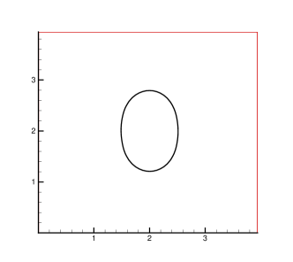
(b) $t=0.01$

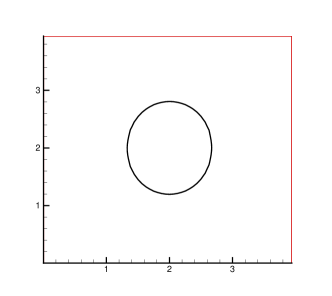
(c) $t=0.05$

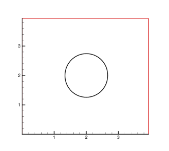
(d) $t=0.1$

Figure 5.1. Towards a circle. Evolution of Willmore of the regularized flow with $\varepsilon=h$ when the initial level set corresponds to an ellipse.

The motion of a square

We now consider an initial data, where the initial level set is a square, that is, it has sharp corners. We report the numerical results in Figure 5.2, which shows the evolution of a square into a circle. We approximate the Willmore flow with $\varepsilon=h$ on a $64\times 64$ grid for the computational domain $\Omega=[0,4]\times[0,4]$. Here, we also adopt a second order semi-implicit Runge-Kutta method with a time step of $\Delta t=0.001h$.

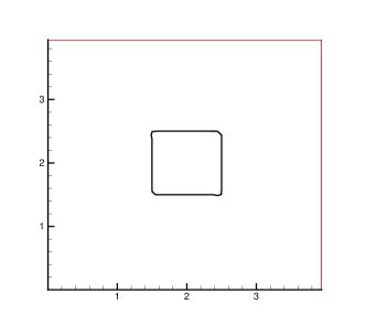
(a) $t=0$

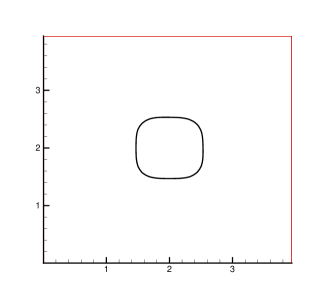
(b) $t=0.0005$

(c) $t=0.001$

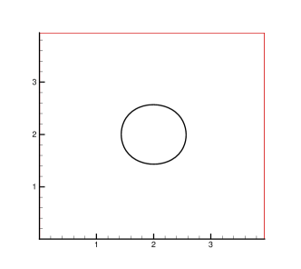
(d) $t=0.002$

Figure 5.2. Towards a circle. Evolution of Willmore of the regularized flow with $\varepsilon=h$ when the initial level set corresponds to a square.

The motion of an asteroid

In Figure 5.3, we present the motion of another non-convex curve with very sharp corners. The numerical methods and parameters are chosen to be the same with those in the previous example. Also the initial asteroid is evolved to be a circle.

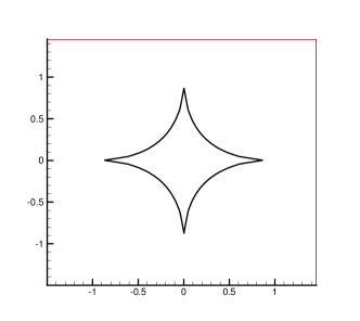
(a) $t=0$

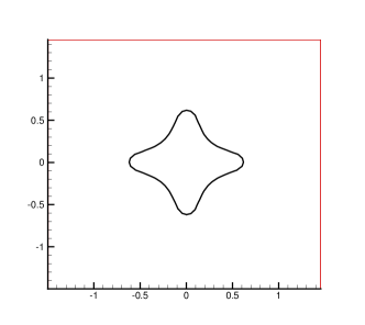
(b) $t=0.0001$

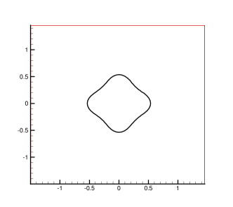
(c) $t=0.0005$

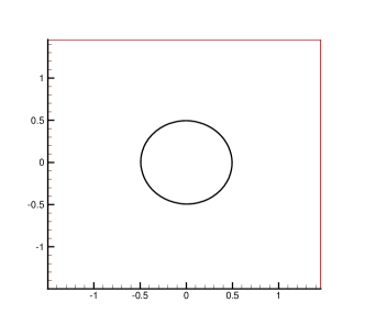
(d) $t=0.005$

Figure 5.3. Towards a circle. Evolution of Willmore of the regularized flow with $\varepsilon=h$ when the initial level set corresponds to an asteroid.

The motion of a singular curve

We consider an initial data, where the initial level set is a singular curve. We report the numerical results in Figure 5.4, which shows the evolution of a singular curve into a circle. We approximate the Willmore flow with $\varepsilon=10h$ and $\varepsilon=10h^{2}$, respectively on a $64\times 64$ grid for the computational domain $\Omega=[-4,4]\times[-4,4]$, which shows similar patterns with different regularization parameter $\varepsilon$.

(a) $\varepsilon=10h$, $t=0$

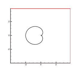
(b) $\varepsilon=10h^{2}$, $t=0$

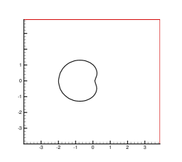
(c) $\varepsilon=10h$, $t=0.0005$

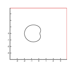
(d) $\varepsilon=10h^{2}$, $t=0.0005$

(e) $\varepsilon=10h$, $t=0.01$

(f) $\varepsilon=10h^{2}$, $t=0.01$

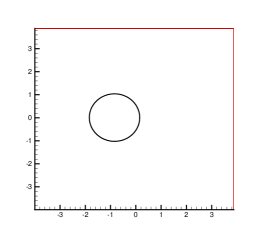
(g) $\varepsilon=10h$, $t=0.1$

(h) $\varepsilon=10h^{2}$, $t=0.1$

Figure 5.4. Towards a circle. Evolution of Willmore of the regularized flow with $\varepsilon=10h$ and $\varepsilon=10h^{2}$ when the initial level set corresponds to a singular curve.

5.3. Topology changes

Finally, in this example, we present two examples to illustrate a topological change under Willmore flow, which is one of the major advantages of level set methods. However, level set methods for this problem suffer from an additional difficulty. The Willmore flow does not have a maximum principle, which leads to that two surfaces both undergoing an evolution by Willmore flow my intersect in finite time. To handle these difficulties, it is important to choose the regularization parameter $\varepsilon$ to avoid a blow up of the gradient of $\phi$ in finite time. In addition, it is important to choose small time steps to temporally resolve the rapid transients that occur at a topological change.

Figure 5.5 presents the merging of two square-like shapes under the level set evolution of Willmore flow. We can see the two square-like shapes merge and eventually evolve to a single circle. Here, we choose $\varepsilon=5h$, and the time step size is $\Delta t=10^{-6}$. Since for such small time step, we use here a first order semi-implicit time marching method. Certainly, we can use explicit Runge-Kutta method here, but because of the severe time step restriction of explicit methods, the time step must be very small, which takes about $\Delta t\approx 10^{-9}$.

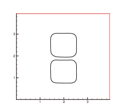
(a) $t=0$

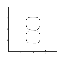
(b) $t=0.0002$

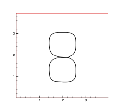
(c) $t=0.00022$

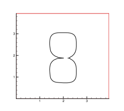
(d) $t=0.00023$

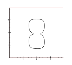
(e) $t=0.00025$

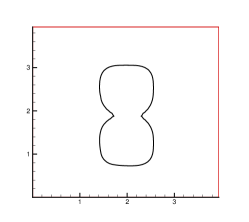
(f) $t=0.0003$

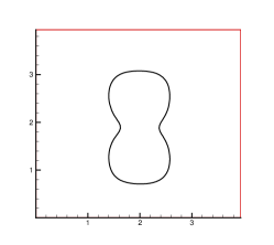
(g) $t=0.0007$

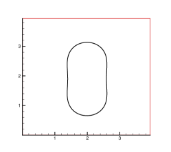
(h) $t=0.01$

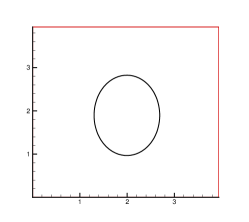
(i) $T=0.05$

Figure 5.5. Topology changes. Two square-like shapes merge under the level set evolution of Willmore flow.

In Figure 5.6, we show another example of topological change. The initial configuration consists of two almost touching surfaces-the inner surface being a circle and the outer surface being an ellipse. We can see a phenomenon of pinching off in Figure 5.6. Here, we also choose $\varepsilon=5h$, and the time step size $\Delta t=10^{-6}$.

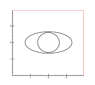
(a) $t=0$

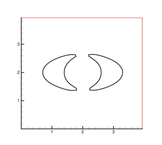
(b) $t=0.00002$

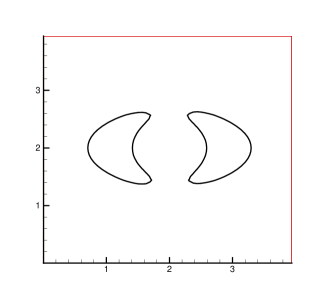
(c) $t=0.0001$

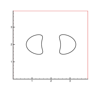
(d) $t=0.001$

Figure 5.6. Topology changes. Two shapes pinch off under the level set evolution of Willmore flow.

6. Concluding remarks

In this work, we have developed a local discontinuous Galerkin method for a level set formulation of Willmore flow. The scheme is mass conservative and energy stable. In the level set method, we are mainly interested in capturing the movement of the interface. Therefore, it is reasonable and natural to combine our local discontinuous Galerkin scheme with $p$-adaptive technique to improve the efficiency of the method. To relax the severe time step restriction of explicit time integration methods for stability and achieve high order temporal accuracy, a semi-implicit Runge-Kutta method is adopted. The equations at the implicit time level are linear and we employ an efficient multigrid solver to solve them. Numerical experiments demonstrate that the proposed methods are efficient for Willmore flow, and the level set method can easily handle topological changes.

References

- [1] M. Beneš, K. Mikula, T. Oberhuber and D. Ševčovič, Comparison study for level set and direct Lagrangian methods for computing Willmore flow of closed planar curves, Computing and visualization in science, 12 (2009), pp.307-317.
- [2] S. Boscarino, F. Filbet and G. Russo, High order semi-implicit schemes for time-dependent partial differential equations, Journal Scientific Computing (2016).
- [3] A. Brandt, Multigrid techniques: 1984 guide with applications to fluid dynamics. GMD-Studien [GMD Studies], 85. Gesellschaft für Mathematik und Datenverarbeitung mbH, St. Augustin, 1984.
- [4] B. Cockburn and C.-W. Shu, TVB Runge-Kutta local projection discontinuous Galerkin finite element method for conservation laws II: general framework, Math. Comp., 52 (1989), pp.411-435.
- [5] B. Cockburn, S.-Y. Lin and C.-W. Shu, TVB Runge-Kutta local projection discontinuous Galerkin finite element method for conservation laws III: one dimensional systems, J. Comput. Phys., 84 (1989), pp.90-113.
- [6] B. Cockburn, S. Hou and C.-W. Shu, The Runge-Kutta local projection discontinuous Galerkin finite element method for conservation laws IV: the multidimensional case, Math. Comp., 54 (1990), pp.545-581.
- [7] B. Cockburn and C.-W. Shu, The Runge-Kutta discontinuous Galerkin method for conservation laws V: multidimensional systems, J. Comput. Phys., 141 (1998), pp.199-224.
- [8] B. Cockburn and C.-W. Shu, The local discontinuous Galerkin method for time-dependent convection-diffusion systems, SIAM J. Numer. Anal., 35 (1998), pp.2440-2463.
- [9] K. Deckelnick and G. Dziuk, Error analysis of a finite element method for the Willmore flow of graphs, Interfaces Free Bound., 8 (2006), pp. 21-46.
- [10] M. Droske and M. Rumpf, A level set formulation for Willmore flow, Interfaces and Free Boundaries, 6 (2004), pp.361-378.
- [11] R. Guo, F. Filbet and Y. Xu Efficient high order semi-implicit time discretization and local discontinuous Galerkin methods for highly nonlinear PDEs , Journal Scientific Computing, (2016).
- [12] T. Oberhuber, Numerical solution for the Willmore flow of graphs, Proceedings of Czech-Japanese Seminar in Applied Mathematics 2005, COE Lect. Note, 3, Kyushu Univ. The 21 Century COE Program, Fukuoka, 2006, pp.126-138.
- [13] S. Osher and J.A. Sethian, Fronts propagating with curvature dependent speed: Algorithms based on Hamilton-Jacobi formulations, J. Comput. Phys., 79 (1988), pp.12-49.
- [14] S. Osher and R. Fedkiw, Level set methods: An overview and some recent results, J. Comput. Phys., 169 (2001), pp.463-502.
- [15] S. Osher and R. Fedkiw, Level set methods and dynamic implicit surfaces, Applied Mathematical Sciences, 153. Springer-Verlag, New York, 2003.
- [16] W. Reed and T. Hill, Triangular mesh methods for the neutron transport equation, Technical report LA-UR-73-479, Los Alamos Scientific Laboratory, Los Alamos, NM, 1973.
- [17] U. Trottenberg, C. Oosterlee and A. Schüller, Multigrid, Academic Press, New York (2005).
- [18] Y. Xia, Y. Xu and C.-W. Shu, Efficient time discretization for local discontinuous Galerkin methods, Discrete Contin. Dyn. Syst. Ser. B, 8 (2007), pp.677-693.
- [19] Y. Xu and C.-W. Shu, Local discontinuous Galerkin method for surface diffusion and Willmore flow of graphs, J. Sci. Comput., 40 (2009), pp.375-390.
- [20] Y. Xu and C.-W. Shu, Local discontinuous Galerkin methods for high-order time-dependent partial differential equations, Commun. Comput. Phys., 7 (2010), pp.1-46.
- [21] J. Yan and S. Osher, Discontinuous Galerkin level set method for interface capturing, UCLA report, 2005.
Francis Filbet
Université de Toulouse III & IUF
UMR5219, Institut de Mathématiques de Toulouse,
118, route de Narbonne
F-31062 Toulouse cedex, FRANCE
e-mail: francis.filbet@math.univ-toulouse.fr
Ruihan Guo
Institut Camille Jordan,
Université Claude Bernard Lyon I,
43 boulevard 11 novembre 1918,
69622 Villeurbanne cedex, France.
e-mail: rguo@math.univ-lyon1.fr.