Screening corrections to the Coulomb crystal elastic moduli

Abstract

Corrections to elastic moduli, including the effective shear modulus, of a solid neutron star crust due to electron screening are calculated. At any given mass density the crust is modelled as a body-centered cubic Coulomb crystal of fully ionized atomic nuclei of a single type with a polarizable charge-compensating electron background. Motion of the nuclei is neglected. The electron polarization is described by a simple Thomas-Fermi model of exponential electron screening. The results of numerical calculations are fitted by convenient analytic formulae. They should be used for precise neutron star oscillation modelling, a rapidly developing branch of stellar seismology.

1 Introduction

Discovery of quasi-periodic oscillations (QPO) in soft gamma-repeaters (Israel et al., 2005; Strohmayer & Watts, 2005; Watts & Strohmayer, 2006) has stimulated interest in studying properties of neutron stars and matter at extreme physical conditions by methods of asteroseismology. The QPO are hypothesized to be related to neutron star vibrations, particularly to torsional vibrations of a solid neutron star crust (Duncan, 1998; Piro, 2005). The crustal oscillation frequencies are determined by elastic moduli of the neutron star crust. The main purpose of the present paper is to provide new results for these quantities under more realistic assumptions about the state of the crustal matter than in previous studies.

The bulk of the outer neutron star crust is made of fully ionized ions in crystalline state, immersed in a nearly uniform strongly degenerate electron gas. More specifically, we suppose that at any given mass density all ions have the same charge $Ze$ and mass $M$ and form a crystal, if the local temperature $T$ falls below the melting temperature $T_{\rm m}=Z^{2}e^{2}/(a\Gamma_{\rm m})$, where $\Gamma_{\rm m}\approx 175$, and $a=(4\pi n/3)^{-1/3}$ is the ion sphere radius ($n$ is the ion number density, $k_{\rm B}=1$). Typically, one assumes that the ion crystal is of the body-centered cubic (bcc) type, as this structure is preferable thermodynamically for a strictly uniform electron background.

In the inner neutron star crust, at densities above the neutron drip density $\rho_{\rm d}\approx 4.3\times 10^{11}$ g cm^-3, in addition to the crystal of ions and electrons, there are neutrons not bound in the atomic nuclei. The details of the neutron interaction with nuclei are not known very well. The motion of nuclei about the crystal lattice nodes may be affected by the presence of neutrons (Chamel, 2012). However, for the purpose of this paper it is irrelevant as we will be concentrating on the static lattice case. At the bottom of the inner crust at densities $\rho\ga 10^{14}$ g cm^-3 there may be a region of nonspherical nuclei, known as “nuclear pasta”, in which the Coulomb crystal model fails (e.g., Pethick & Potekhin, 1998).

The state of the electron subsystem depends on the matter density. We shall limit ourselves to such not too low densities, where electrons are degenerate and ions are completely pressure ionized ($\rho\ga 10AZ$ g cm^-3, where $A$ is the number of nucleons per nucleus, which is equal to the nucleus mass number in the outer crust; see for discussion Pethick & Ravenhall, 1995; Haensel, Potekhin & Yakovlev, 2007). The degenerate electrons are very energetic (at $\rho\gg 10^{6}$ g cm^-3 they become ultrarelativistic) and it is typically considered a good approximation to treat them as a constant and uniform charge background. In this case, the ion-electron system is called a one-component plasma (or a Coulomb crystal, if crystallization is assumed).

However, in reality, electrons respond to the ion charge density, which results in a screening effect. The strength of this electron polarization can be characterized by the screening parameter $\kappa a$, where $\kappa$ is the Thomas-Fermi wavenumber:

$$\kappa a=2k_{\rm F}a\sqrt{\alpha/(\pi\beta)}\approx 0.19Z^{1/3}\beta^{-1/2}~{}.$$ (1)

In this case $\beta=v_{\rm F}/c$, $v_{\rm F}$ and $k_{\rm F}$ are the electron Fermi velocity and wavevector, respectively, $\alpha$ is the fine-structure constant, and $c$ is the speed of light. Furthermore, $\beta=x_{\rm r}/\sqrt{1+x^{2}_{\rm r}}$, where $x_{\rm r}$ is the electron relativity parameter:

$$x_{\rm r}=\frac{\hbar k_{\rm F}}{mc}\approx 1.009\left(\frac{\rho_{6}Z}{A}\right)^{1/3}~{},$$ (2)

where $m$ is the electron mass and $\rho_{6}$ is the mass density in units of $10^{6}$ g cm^-3. The electron polarization is not very weak even in the inner neutron star crust, where electrons are ultrarelativistic. For instance, for $Z=40$, $\kappa a\approx 0.65$. In the outer neutron star crust, the screening parameter decreases with decrease of $Z$ but increases with decrease of the mass density (i.e. decrease of the electron relativity degree). At sufficiently low density, the screening parameter exceeds 1, screening becomes strong and full ionization assumption is eventually violated.

The main purpose of this paper is to study the elastic moduli of the Coulomb crystal taking into account the electron polarization. The groundwork for this problem was laid down by Fuchs (1936), who calculated the elastic moduli of the static bcc Coulomb lattice. Ogata & Ichimaru (1990) calculated the elastic moduli of the bcc Coulomb crystal taking into account the motion of ions about their lattice nodes. They have also introduced in astrophysics the concept of shear wave directional averaging and an effective shear modulus of polycrystalline neutron star crust, which is used extensively nowdays. In that work the moduli were found numerically with the aid of Monte Carlo simulations (e.g., Brush et al., 1966). By the nature of the method, the motion of ions was treated classically.

Horowitz & Hughto (2008) calculated the effective shear modulus of the Coulomb crystal taking into account electron screening in the Thomas-Fermi model. These authors restricted themselves to a specific nucleus charge number and mass density and have not reported on the dependence of the screening correction on these parameters. The calculation was done numerically using the molecular dynamics method. Again, the motion of ions was strictly classic.

The effective shear modulus and the Huang elastic shear coefficient $S_{1212}$ of the one-component plasma crystal with account of the ion motion was calculated semi-analytically by Baiko (2011). In that paper thermodynamic perturbation theory was employed and the ion motion was included in the harmonic lattice model framework. Unlike numerical methods of Ogata & Ichimaru (1990) and Horowitz & Hughto (2008) this approach allowed one to capture quantum effects. The quantum effects were found to be rather moderate and of greater importance for lighter elements at higher densities.

The electron polarization correction to the static Coulomb crystal effective shear modulus was calculated by Baiko (2012). In this paper, screening was described in the linear response formalism. Two models of the relativistic electron gas response were considered, the Thomas-Fermi model and the zero temperature random phase approximation with specific formulae for the dielectric function derived by Jancovici (1962). The results were on average compatible with each other, but the calculations with the Jancovici screening model revealed sharp singularities in the dependence of the effective shear modulus on the charge number $Z$ treated as a continuous variable. The singularities were more pronounced at lower densities. Consequently, at certain integer $Z$ and low densities these results deviated significantly from the Thomas-Fermi theory. At the same time, neither corrections to the individual elastic coefficients nor details of the calculations were reported. Based on the numerical results of Baiko (2012), Kobyakov & Pethick (2013) produced a fit for the effective shear modulus screening correction in the Thomas-Fermi model.

In their subsequent work, Kobyakov & Pethick (2015) have re-evaluated the concept of the effective shear modulus as it is used in astrophysics. Instead of the shear wave directional averaging, they have proposed to use a self-consistent theory (e.g., deWit, 2008), developed to describe elastic properties of polycrystalline matter with randomly oriented perfect crystallites. In this theory, the effective shear modulus is given by a nonlinear expression containing all the individual elastic moduli of the perfect lattice.

The goal of the present work is to extend the work of Baiko (2012) as well as to provide necessary details of these calculations. In particular, we report on the screening contributions to all second order elastic coefficients of the static crystal with the bcc lattice. We treat electron polarization perturbatively (perturbative calculations based on the one-component plasma model fail at $\kappa a\gtrsim 1$). We propose simple analytic formulae for screening corrections to all the elastic moduli in the Thomas-Fermi model. We do not analyze modification due to screening of the ion motion contribution obtained by Baiko (2011) as this effect would produce too small a correction to the total elastic moduli.

Besides neutron star crusts, the Coulomb crystals with polarizable electron background are expected to form in solid cores of white dwarfs, to which the present results also apply.

2 General formalism

Huang elastic moduli $S_{\alpha\beta\gamma\lambda}$ are the second order expansion coefficients of the Helmholtz free energy per unit mass in powers of the displacement gradients, multiplied by the mass density in the initial, non-deformed configuration (e.g., Eq. (5.1) of Wallace, 1967). They are also known as the equation of motion coefficients, as they enter the equation of motion of a material, deformed with respect to an initial configuration, characterized by an arbitrary uniform stress.

If a material is under an isotropic initial stress, such as hydrostatic pressure, it is more convenient to use Birch elastic moduli or the stress-strain coefficients $B_{\alpha\beta\gamma\lambda}$ (in the nomenclature of Wallace, 1967). The convenience stems from the fact that under the isotropic initial stress these coefficients possess the complete Voigt symmetry and, at the same time, can be used in the equation of motion in place of the Huang coefficients. The Birch coefficients had been generalized to the case of a material of an arbitrary symmetry under an arbitrary initial stress in Barron & Klein (1965), where they were denoted as $\mathring{c}_{\alpha\beta\gamma\lambda}$. They had been reintroduced again in Marcus et al. (2002) as second order expansion coefficients of the Gibbs free energy in powers of the strain parameters. Due to their Voigt symmetry, Voigt notation (with only two indices, e.g., Wallace, 1967) is usually used for them. For instance, for the cubic symmetry, the only independent coefficients are $B_{1111}=\mathring{c}_{1111}=c_{11}$, $B_{1122}=\mathring{c}_{1122}=c_{12}$, $B_{1212}=\mathring{c}_{1212}=c_{44}$. (Let us note, that under an anisotropic initial stress the Birch coefficients lose the Voigt symmetry, are no longer equivalent to the equation of motion coefficients and cannot be obtained from the Gibbs free energy, as the latter does not exist.)

The relationships between the Huang and Birch coefficients are well-known (e.g., Eqs. (2.24) and (2.36) of Wallace, 1967, for an arbitrary initial stress or Eqs. (2.55) and (2.56) for isotropic pressure). In particular, for the case of initial isotropic pressure $P$ and for a material possessing the cubic symmetry $c_{11}=S_{1111}$, $c_{12}=S_{1122}+P$, $c_{44}=S_{1212}$. (Additionally, $S_{1221}=S_{1212}+P$.) These formulae apply for any partial contribution to these coefficients (i.e., due to static lattice, electron screening, phonons etc).

The Huang elastic moduli of static (st) bcc Coulomb lattice with a uniform background of opposite charge are (Fuchs, 1936)

$$S^{\rm st}_{1111} = -0.36553930\,S_{0}$$

$$S^{\rm st}_{1122} = -0.11587344\,S_{0}$$

$$S^{\rm st}_{1221} = -0.11587344\,S_{0}$$

$$S^{\rm st}_{1212} = S^{\rm st}_{1221}-P^{\rm st}=0.18276965\,S_{0}~{},$$ (3)

where $S_{0}=nZ^{2}e^{2}/a$; see also Baiko (2011). The effective shear modulus obtained via the directional averaging procedure of Ogata & Ichimaru (1990) reads

$$\mu^{\rm st}_{\rm eff}=\frac{1}{5}(S^{\rm st}_{1111}-S^{\rm st}_{1122}-S^{\rm st}_{1221}+4S^{\rm st}_{1212})=0.1194572\,S_{0}~{},$$ (4)

and the self-consistent shear modulus of Kobyakov & Pethick (2015) becomes (assuming the dominance of the electron bulk modulus over all the other elastic coefficients)

$$\mu^{\rm st}_{\rm eff,sc}\approx 0.093\,S_{0}~{}.$$ (5)

Polarizability of the electron background results in a contribution $F_{\epsilon}$ to the system Helmholtz free energy per ion. We describe this effect in the linear response formalism assuming that the electrons adjust instantaneously to the ion configuration. Thus, the electron response can be described by a static ($\omega=0$) longitudinal dielectric function $\epsilon(q)$. Assuming further that all ions are fixed at their lattice nodes $\bm{R}$ (and thus neglecting modification of the ion motion term by the polarization) we obtain:

$$F_{\epsilon} = \frac{Z^{2}e^{2}}{2}\int\frac{{\rm d}\bm{q}}{(2\pi)^{3}}\frac{4\pi}{q^{2}}\left[\frac{1}{\epsilon(q)}-1\right]$$ (6)

$$\times \left(\sum_{\bm{R}}\exp{(i\bm{q}\bm{R})}-n\int{\rm d}\bm{r}\exp{(i\bm{q}\bm{r})}\right)$$

(e.g., Hubbard & Slattery, 1971; Yakovlev & Shalybkov, 1989).

Introducing uniform deformation with constant displacement gradients $u_{\alpha\beta}$, we replace $R_{\alpha}\to R_{\alpha}+u_{\alpha\beta}R_{\beta}$ and $r_{\alpha}\to r_{\alpha}+u_{\alpha\beta}r_{\beta}$ in the exponentials in Eq. (6). Also we have to take into account a dependence of $\epsilon(q)$ on the density, which changes under the deformation by $\delta n\approx n(-u_{\alpha\alpha}+0.5u_{\alpha\alpha}u_{\beta\beta}+0.5u_{\alpha\beta}u_{\beta\alpha})$. [We can also integrate over the new variable $r_{\alpha}+u_{\alpha\beta}r_{\beta}$ and insert the new ion number density in front of the integral in the second line of Eq. (6), but these two modifications cancel each other out.] Accordingly, $F_{\epsilon}\to F_{\epsilon}+\delta F_{\epsilon}$, where $\delta F_{\epsilon}$ can be expanded in powers of the displacement gradients:

$$n\delta F_{\epsilon} = \frac{nZ^{2}e^{2}}{2}\left(\sum_{\bm{R}}-\int n{\rm d}\bm{R}\right)\int\frac{{\rm d}\bm{q}}{(2\pi)^{3}}\frac{4\pi}{q^{2}}$$ (7)

$$\times \left\{u_{\alpha\beta}\left(R_{\beta}\frac{\partial}{\partial R_{\alpha}}-\delta_{\alpha\beta}n\frac{\partial}{\partial n}\right)\right.$$

$$+ \frac{1}{2}u_{\alpha\beta}u_{\gamma\lambda}\left[R_{\beta}R_{\lambda}\frac{\partial^{2}}{\partial R_{\alpha}\partial R_{\gamma}}-2\delta_{\gamma\lambda}nR_{\beta}\frac{\partial^{2}}{\partial n\partial R_{\alpha}}\right.$$

$$+ \left.\left.(\delta_{\alpha\beta}\delta_{\gamma\lambda}+\delta_{\alpha\lambda}\delta_{\beta\gamma})n\frac{\partial}{\partial n}+\delta_{\alpha\beta}\delta_{\gamma\lambda}n^{2}\frac{\partial^{2}}{\partial n^{2}}\right]+\ldots\right\}$$

$$\times \left[\frac{1}{\epsilon(q)}-1\right]\exp{(i\bm{q}\bm{R})}~{},$$

where we have renamed the integration variable as $\bm{R}$ for brevity of notation, while $\sum_{\bm{R}}$ is over all lattice vectors of the non-deformed crystal. The screening (scr) contribution to the isothermal Huang elastic coefficient $S^{\rm scr}_{\alpha\beta\gamma\lambda}$ is the coefficient of the $u_{\alpha\beta}u_{\gamma\lambda}/2$ term. The factor multiplied by $u_{\alpha\beta}$ in the first order term is $-P^{\rm scr}\delta_{\alpha\beta}$, i.e. the screening contribution to (minus) pressure. If $[1/\epsilon-1]$ is replaced by $1$, then the same factors yield the respective static lattice contributions. In this case, all the terms containing $\partial/\partial n$ vanish. Then it becomes obvious that $S^{\rm st}_{1122}=S^{\rm st}_{1221}$ in accordance with Eq. (3) (this does not hold true for the screening contributions). The relationship $S_{1221}=S_{1212}+P$ for both static and screening contributions can be seen from the fact that at fixed $\bm{R}$ the $\bm{q}$-integral (before applying the operator in curly brackets) is a function of $R^{2}$ only. Then

$$R_{2}^{2}\frac{\partial^{2}}{\partial R_{1}^{2}} = 4R_{1}^{2}R_{2}^{2}\frac{\partial^{2}}{\partial(R^{2})^{2}}+2R_{1}^{2}\frac{\partial}{\partial(R^{2})}$$ (8)

$$R_{1}R_{2}\frac{\partial^{2}}{\partial R_{1}\partial R_{2}} = 4R_{1}^{2}R_{2}^{2}\frac{\partial^{2}}{\partial(R^{2})^{2}}$$ (9)

$$R_{1}\frac{\partial}{\partial R_{1}} = 2R_{1}^{2}\frac{\partial}{\partial(R^{2})}$$ (10)

(where subscripts indicate Cartesian components). In this case, the derivative Eq. (8) contributes to $S_{1212}$, the derivative Eq. (9) contributes to $S_{1221}$, while the derivative Eq. (10) contributes to $-P$. Additionally, $S^{\rm scr}_{1221}$ contains a term with $\partial/\partial n$, which is absent in $S^{\rm scr}_{1212}$, but is present in $P^{\rm scr}$.

It is also useful to write this expansion in reciprocal space:

$$\delta F_{\epsilon} = \frac{4\pi nZ^{2}e^{2}}{2}\sideset{}{{}^{\prime}}{\sum}_{\bm{G}}\left\{u_{\alpha\beta}\left(-\frac{\partial}{\partial G_{\beta}}G_{\alpha}-\delta_{\alpha\beta}n\frac{\partial}{\partial n}\right)\right.$$ (11)

$$+ \frac{1}{2}u_{\alpha\beta}u_{\gamma\lambda}\left[\frac{\partial^{2}}{\partial G_{\beta}\partial G_{\lambda}}G_{\alpha}G_{\gamma}+2\delta_{\gamma\lambda}n\frac{\partial^{2}}{\partial n\partial G_{\beta}}G_{\alpha}\right.$$

$$+ \left.\left.(\delta_{\alpha\beta}\delta_{\gamma\lambda}+\delta_{\alpha\lambda}\delta_{\beta\gamma})n\frac{\partial}{\partial n}+\delta_{\alpha\beta}\delta_{\gamma\lambda}n^{2}\frac{\partial^{2}}{\partial n^{2}}\right]+\ldots\right\}$$

$$\times \frac{1}{G^{2}}\left[\frac{1}{\epsilon(G)}-1\right]~{}.$$

The $\bm{G}$-summation in this formula is over all non-zero reciprocal lattice vectors.

The derivatives featuring in Eq. (11) can be easily evaluated with the following results:

$$\frac{\partial}{\partial n}\left[\frac{1}{\epsilon(G)}-1\right]=-\frac{\dot{\epsilon}}{\epsilon^{2}}~{},$$

$$\frac{\partial^{2}}{\partial n^{2}}\left[\frac{1}{\epsilon(G)}-1\right]=\frac{2\dot{\epsilon}^{2}}{\epsilon^{3}}-\frac{\ddot{\epsilon}}{\epsilon^{2}}~{},$$

$$\frac{\partial}{\partial G_{\beta}}\frac{G_{\alpha}}{G^{2}}\left[\frac{1}{\epsilon(G)}-1\right]$$

$$~{}~{}=~{}\left(\frac{\delta_{\alpha\beta}}{G^{2}}-\frac{2G_{\alpha}G_{\beta}}{G^{4}}\right)\left[\frac{1}{\epsilon(G)}-1\right]-\frac{G_{\alpha}G_{\beta}}{G^{3}}\frac{\epsilon^{\prime}}{\epsilon^{2}}~{},$$

$$\frac{\partial^{2}}{\partial G_{\beta}\partial G_{\lambda}}\frac{G_{\alpha}G_{\gamma}}{G^{2}}\left[\frac{1}{\epsilon(G)}-1\right]$$

$$~{}~{}=~{}(\delta_{\alpha\lambda}\delta_{\beta\gamma}+\delta_{\alpha\beta}\delta_{\gamma\lambda})\frac{1}{G^{2}}\left(\frac{1}{\epsilon}-1\right)$$

$$~{}~{}-~{}(\delta_{\beta\lambda}G_{\alpha}G_{\gamma}+\delta_{\beta\gamma}G_{\alpha}G_{\lambda}+\delta_{\alpha\beta}G_{\gamma}G_{\lambda}$$

$$~{}~{}+~{}\delta_{\alpha\lambda}G_{\beta}G_{\gamma}+\delta_{\gamma\lambda}G_{\alpha}G_{\beta})\frac{1}{G^{2}}\left[\frac{2}{G^{2}}\left(\frac{1}{\epsilon}-1\right)+\frac{\epsilon^{\prime}}{G\epsilon^{2}}\right]$$

$$~{}~{}+~{}\frac{G_{\alpha}G_{\beta}G_{\gamma}G_{\lambda}}{G^{4}}\left[\frac{8}{G^{2}}\left(\frac{1}{\epsilon}-1\right)+\frac{5\epsilon^{\prime}}{G\epsilon^{2}}+\frac{2\epsilon^{\prime 2}}{\epsilon^{3}}-\frac{\epsilon^{\prime\prime}}{\epsilon^{2}}\right],$$

$$\frac{\partial^{2}}{\partial n\partial G_{\beta}}\frac{G_{\alpha}}{G^{2}}\left[\frac{1}{\epsilon(G)}-1\right]$$

$$~{}~{}=~{}-\frac{\delta_{\alpha\beta}\dot{\epsilon}}{G^{2}\epsilon^{2}}+\frac{G_{\alpha}G_{\beta}}{G^{2}}\left(\frac{2\dot{\epsilon}}{G^{2}\epsilon^{2}}+\frac{2\dot{\epsilon}\epsilon^{\prime}}{G\epsilon^{3}}-\frac{\dot{\epsilon}^{\prime}}{G\epsilon^{2}}\right),$$ (12)

where a dot over $\epsilon$ means the derivative with respect to $n$ (the electron density is $Zn$), while a prime over $\epsilon$ means the derivative with respect to $G$.

3 Calculations with the Thomas-Fermi dielectric function

The Thomas-Fermi (TF) dielectric function $\epsilon_{\rm TF}(q)=1+\kappa^{2}/q^{2}$ describes exponential screening of the Coulomb potential with the screening length equal to $1/\kappa$. In principle, one can use Eqs. (11) and (12) to find the screening contributions to the Huang coefficients. However, $(1/\epsilon_{\rm TF})-1\sim q^{-2}$ at large $q$ and the expression under the three-dimensional reciprocal lattice sum would decay only as $q^{-4}$. Consequently, the convergence would be very slow.

Fortunately, the problem can be reformulated using the “screened” Ewald technique identical to that used in Baiko (2002). The final practical formula for $S^{\rm scr}_{\alpha\beta\gamma\lambda}$ in the Thomas-Fermi approximation is given in the Appendix, Eq. (23). Its derivation is based on several simple ideas. First, we note that a contribution to $S^{\rm scr}_{\alpha\beta\gamma\lambda}$, corresponding to a given $\bm{R}$, can be written as

$$\frac{Z^{2}e^{2}}{2}\left[R_{\beta}R_{\lambda}\frac{\partial^{2}}{\partial R_{\alpha}\partial R_{\gamma}}-2\delta_{\gamma\lambda}nR_{\beta}\frac{\partial^{2}}{\partial n\partial R_{\alpha}}\right.$$ (13)

$$+ \left.(\delta_{\alpha\beta}\delta_{\gamma\lambda}+\delta_{\alpha\lambda}\delta_{\beta\gamma})n\frac{\partial}{\partial n}+\delta_{\alpha\beta}\delta_{\gamma\lambda}n^{2}\frac{\partial^{2}}{\partial n^{2}}\right]$$

$$\times \frac{1}{R}[\exp{(-\kappa R)}-1].$$

[Interestingly, the $\bm{R}=0$ term produces non-zero contributions to $S^{\rm scr}_{1111}$, $S^{\rm scr}_{1122}$ and $S^{\rm scr}_{1221}$, but not to the shear coefficient $S^{\rm scr}_{1212}$. This is the $S^{(1)}$ term in Eq. (23).]

Then we use the following standard integral:

$$\frac{e^{-\kappa R}-1}{R}=\frac{2}{\sqrt{\pi}}\int^{\infty}_{0}{\rm d}\rho e^{-\rho^{2}R^{2}}\left(e^{-\kappa^{2}/(4\rho^{2})}-1\right)~{},$$ (14)

and split it as $\int^{\infty}_{0}=\int^{\cal A}_{0}+\int^{\infty}_{\cal A}$, where $0<{\cal A}<\infty$ but otherwise arbitrary. The integral $\int^{\infty}_{\cal A}$ may be expressed via the complementary error functions ${\rm erfc}({\cal A}R\pm\kappa/(2{\cal A}))$ which decay very rapidly at large $R$. We differentiate them as prescribed by Eq. (13) and this results in contributions $S^{(2)}$ and $S^{(3)}$ in Eq. (23) for $\int{\rm d}\bm{R}$ and $\sum_{\bm{R}\neq 0}$, respectively. In $S^{(3)}$ it is sufficient to sum over very few first shells of lattice vectors $\bm{R}$ to achieve convergence.

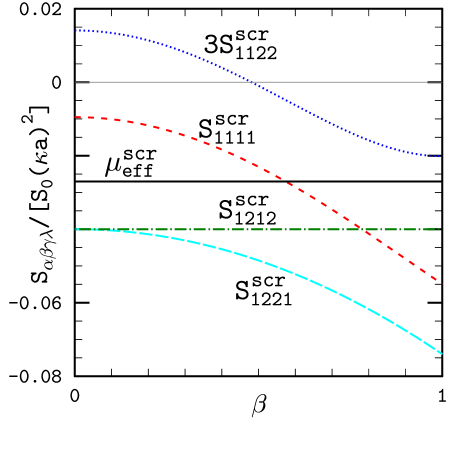
Figure 1: Screening corrections to elastic moduli calculated using $\epsilon_{\rm TF}$.

Clearly, this procedure relies on the fact that ${\cal A}>0$, and a different treatment of the integral $\int^{\cal A}_{0}$ is needed. We substitute the well-known formula

$$\exp{\left(-\rho^{2}R^{2}\right)}=\int\frac{{\rm d}\bm{q}}{(2\pi)^{3}}\frac{\pi\sqrt{\pi}}{\rho^{3}}\exp{\left[i\bm{q}\bm{R}-q^{2}/(4\rho^{2})\right]}$$ (15)

in Eq. (14). After that, for instance, $R_{\beta}R_{\lambda}\partial^{2}/(\partial R_{\alpha}\partial R_{\gamma})$ in Eq. (13) becomes $q_{\alpha}q_{\gamma}\partial^{2}/(\partial q_{\beta}\partial q_{\lambda})$. Summation over $\bm{R}$ then yields a series of delta-functions in reciprocal space via the identity $\sum_{\bm{R}}\exp{(i\bm{q}\bm{R})}=(2\pi)^{3}n\sum_{\bm{G}}\delta(\bm{q}-\bm{G})$. [The $\bm{R}=0$ term now has to be subtracted as it is already present in the form of $S^{(1)}$. This results in the $S^{(4)}$ term in Eq. (23). If ${\cal A}\to\infty$, $S^{(4)}\to-S^{(1)}$ as it should be.] The $\bm{q}$-integral is then taken with the aid of the integration by parts and the delta-functions. The remaining $\int^{\cal A}_{0}{\rm d}\rho$ turns out to be elementary and the result (the $S^{(5)}$ term) contains the rapidly decaying (for ${\cal A}<\infty$) function $\exp{[-(G^{2}+\kappa^{2})/(4{\cal A}^{2})]}$. It is again sufficient to sum over very few first shells of reciprocal lattice vectors $\bm{G}$ to achieve convergence.

Using Eq. (23), we have calculated the screening corrections to all Huang elastic coefficients. Since these are perturbative calculations, only the lowest order terms in $\kappa a$ are described correctly. They are $\propto(\kappa a)^{2}$ and our main results can be summarized as

$$S^{\rm scr}_{1111} = -(0.0095+0.057\beta^{2}-0.0116\beta^{4})\,(\kappa a)^{2}\,S_{0}~{},$$

$$S^{\rm scr}_{1122} = (0.0047-0.023\beta^{2}+0.0116\beta^{4})\,(\kappa a)^{2}\,S_{0}~{},$$

$$S^{\rm scr}_{1221} = -(0.04+0.034\beta^{2})\,(\kappa a)^{2}\,S_{0}~{},$$

$$S^{\rm scr}_{1212} = c^{\rm scr}_{44}=-0.04\,(\kappa a)^{2}\,S_{0}~{}.$$ (16)

The dependence of some coefficients on $\beta$ stems from the dielectric function dependence on $n$ and variation of the latter for certain types of deformations. These coefficients are shown in Fig. 1. The $S^{\rm scr}_{1122}$ coefficient is additionally multiplied by $3$ to improve the figure readability. The screening correction to the effective shear modulus obtained via the averaging procedure is

$$\mu^{\rm scr}_{\rm eff} = \frac{1}{5}(S^{\rm scr}_{1111}-S^{\rm scr}_{1122}-S^{\rm scr}_{1221}+4S^{\rm scr}_{1212})$$ (17)

$$= -0.027\,(\kappa a)^{2}\,S_{0}~{}.$$

Finally, we have expanded the nonlinear expression of Kobyakov & Pethick (2015) for the self-consistent effective shear modulus and obtained the screening correction to it as

$$\mu^{\rm scr}_{\rm eff,sc}=-0.022\,(\kappa a)^{2}\,S_{0}~{}.$$ (18)

The polarization contributions to the Huang shear coefficient $S_{1212}$ and the effective shear moduli are, as expected, negative. This means that screening reduces lattice resistance to a shear strain. Also they do not contain contributions associated with the density dependence of the dielectric function. Naturally, the polarization corrections Eqs. (16)—(18) are smaller than the electrostatic elastic moduli Eqs. (3)—(5) within the limits of validity of the perturbative treatment of screening. The fit (17) has already been proposed by Kobyakov & Pethick (2013) based on the numerical data of Baiko (2012). However, their coefficient in Eq. (17) is $\sim 20\%$ greater than ours due to a minor numerical error on their part. Results (16) and (18) are new.

It is also convenient to reformulate our results in terms of the pressure

$$P^{\rm scr}=S^{\rm scr}_{1221}-S^{\rm scr}_{1212}=-0.034\beta^{2}\,(\kappa a)^{2}\,S_{0}~{},$$ (19)

bulk modulus

$$\frac{1}{3}(c^{\rm scr}_{11}+2c^{\rm scr}_{12}) = \frac{1}{3}(S^{\rm scr}_{1111}+2S^{\rm scr}_{1122}+2S^{\rm scr}_{1221}-2S^{\rm scr}_{1212})$$ (20)

$$= -(0.057\beta^{2}-0.0116\beta^{4})\,(\kappa a)^{2}\,S_{0}~{},$$

and

$$c^{\rm scr}_{11}-c^{\rm scr}_{12} = S^{\rm scr}_{1111}-S^{\rm scr}_{1122}-S^{\rm scr}_{1221}+S^{\rm scr}_{1212}$$ (21)

$$= -0.0142\,(\kappa a)^{2}\,S_{0}~{}.$$

From the results reported so far one may gain an impression that the screening corrections can become very large relative to the pure Coulomb values of the elastic moduli at low mass densities and at $Z\gg 1$. In this regime our perturbative method does not work. For instance, at $x_{\rm r}=0.2$ and $Z=26$, $\kappa a\approx 1.3$. However, in this regime we expect an onset of partial ionization. In this case, matter can be approximately described as a Coulomb system with an effective ion charge $Z_{\rm eff}<Z$. This effective charge will result in reduced effective values of $\kappa a$ and $S_{0}$ to be used in Eqs. (3)—(5) and (16)—(18).

4 Conclusion

We have calculated electron polarization corrections to elastic moduli of Coulomb crystals in neutron star crust. The effect was described by the Thomas-Fermi model of exponential electron screening.

Combining with Eqs. (45) and (46) of Baiko (2011), we can now write expressions for the total effective shear moduli $\mu^{\rm tot}_{\rm eff}$, $\mu^{\rm tot}_{\rm eff,sc}$ and the elastic shear coefficient $S^{\rm tot}_{1212}$ including the effects of ion motion and electron screening (unfortuantely, the ion motion contribution is presently not available for $\mu^{\rm tot}_{\rm eff,sc}$):

$$S^{\rm tot}_{1212} = [0.18276965-0.04(\kappa a)^{2}]\,S_{0}$$

$$- \left[0.2057+439\left(\frac{T}{T_{\rm p}}\right)^{3}\right]^{1/3}nT_{\rm p}~{},$$

$$\mu^{\rm tot}_{\rm eff} = [0.1194572-0.027(\kappa a)^{2}]\,S_{0}$$

$$- \left[0.05008+136.6\left(\frac{T}{T_{\rm p}}\right)^{3}\right]^{1/3}nT_{\rm p}~{},$$

$$\mu^{\rm tot}_{\rm eff,sc} = [0.093-0.022(\kappa a)^{2}]\,S_{0}~{},$$ (22)

where $T_{\rm p}=\hbar\sqrt{4\pi nZ^{2}e^{2}/M}\approx 7.8\times 10^{6}(Z/A)\sqrt{\rho_{6}X}$ K is the ion plasma temperature. In this case $X=A/A_{\rm N}$, where $A_{\rm N}$ is the number of nucleons bound in a nucleus ($A_{\rm N}=A$ in the outer crust). We would like to emphasize that Eqs. (22) do not take into account details of “free” neutron interactions with nuclei in the inner neutron star crust. Here it is assumed that these effects result in an effective (increased) nucleus mass and a renormalized plasma frequency.

Appendix A

In the Thomas-Fermi approximation

$$S^{\rm scr}_{\alpha\beta\gamma\lambda} = \frac{nZ^{2}e^{2}}{2}\sum_{i=1}^{5}S^{(i)}_{\alpha\beta\gamma\lambda}~{},$$ (23)

$$S^{(1)}_{\alpha\beta\gamma\lambda} = -\delta_{\alpha\beta}\delta_{\gamma\lambda}(\kappa^{1}_{1}+\kappa^{1}_{2})-\delta_{\alpha\lambda}\delta_{\beta\gamma}\kappa^{1}_{1}~{},$$

$$S^{(2)}_{\alpha\beta\gamma\lambda} = -\frac{\pi n}{{\cal A}^{2}}\left[\delta_{\alpha\beta}\delta_{\gamma\lambda}\left(1+3n\frac{{\rm d}}{{\rm d}n}+n^{2}\frac{{\rm d}^{2}}{{\rm d}n^{2}}\right)\right.$$

$$+ \left.\delta_{\alpha\lambda}\delta_{\beta\gamma}\left(1+n\frac{{\rm d}}{{\rm d}n}\right)\right]F(u)~{},$$

$$S^{(3)}_{\alpha\beta\gamma\lambda} = \sideset{}{{}^{\prime}}{\sum}_{\bm{R}}\left[R_{\beta}R_{\lambda}\frac{\partial^{2}}{\partial R_{\alpha}\partial R_{\gamma}}-2\delta_{\gamma\lambda}nR_{\beta}\frac{\partial^{2}}{\partial n\partial R_{\alpha}}\right.$$

$$+ \left.(\delta_{\alpha\beta}\delta_{\gamma\lambda}+\delta_{\alpha\lambda}\delta_{\beta\gamma})n\frac{\partial}{\partial n}+\delta_{\alpha\beta}\delta_{\gamma\lambda}n^{2}\frac{\partial^{2}}{\partial n^{2}}\right]$$

$$\times \left\{\frac{{\cal A}}{2x}[E_{+}(x,y)+E_{-}(x,y)]-\frac{{\cal A}}{x}{\rm erfc}(x)\right\}~{},$$

$$S^{(4)}_{\alpha\beta\gamma\lambda} = \frac{\delta_{\alpha\beta}\delta_{\gamma\lambda}}{2\kappa}\left[E_{+}(0,y)\left(\kappa^{2}_{1}+\kappa^{2}_{2}-\frac{\kappa^{2}_{1}\kappa^{1}_{1}}{\kappa}\right)\right.$$

$$- \left.\frac{\kappa^{2}_{1}\kappa^{1}_{1}}{{\cal A}\sqrt{\pi}}\exp{(-u)}\right]+\frac{\delta_{\alpha\lambda}\delta_{\beta\gamma}}{2\kappa}E_{+}(0,y)\kappa^{2}_{1}~{},$$

$$S^{(5)}_{\alpha\beta\gamma\lambda} = \frac{\pi n}{{\cal A}^{2}}\sideset{}{{}^{\prime}}{\sum}_{\bm{G}}\left[\frac{\partial^{2}}{\partial G_{\beta}\partial G_{\lambda}}G_{\alpha}G_{\gamma}+2\delta_{\gamma\lambda}nG_{\alpha}\frac{\partial^{2}}{\partial n\partial G_{\beta}}\right.$$

$$+ \left.(3\delta_{\alpha\beta}\delta_{\gamma\lambda}+\delta_{\alpha\lambda}\delta_{\beta\gamma})n\frac{\partial}{\partial n}+\delta_{\alpha\beta}\delta_{\gamma\lambda}n^{2}\frac{\partial^{2}}{\partial n^{2}}\right]$$

$$\times [D(g,u)-D(g,0)]~{},$$

where primes mean that the $\bm{R}=0$ and $\bm{G}=0$ terms in the lattice sums must be omitted. Furthermore,

$$F(u) = \frac{1}{u}\left[1-\exp{(-u)}\right]-1~{},$$

$$E_{\pm}(x,y) = \exp{(\pm 2xy)}{\rm erfc}(x\pm y)~{},$$

$${\rm erfc}(x) = E_{\pm}(x,0)~{},$$

$$D(g,u) = \frac{1}{g+u}\exp{(-g-u)}~{},$$

$$u = y^{2}~{},~{}~{}~{}x={\cal A}R~{},$$

$$y = \frac{\kappa}{2{\cal A}}~{},~{}~{}~{}g=\frac{G^{2}}{4{\cal A}^{2}}~{},$$

$$n\frac{{\rm d}F}{{\rm d}n} = \frac{{\rm d}F}{{\rm d}u}\frac{\kappa^{2}_{1}}{4{\cal A}^{2}}~{},$$

$$n\frac{{\rm d}^{2}F}{{\rm d}n^{2}} = \frac{{\rm d}^{2}F}{{\rm d}u^{2}}\frac{(\kappa^{2}_{1})^{2}}{16{\cal A}^{4}}+\frac{{\rm d}F}{{\rm d}u}\frac{\kappa^{2}_{2}}{4{\cal A}^{2}}~{},$$

$$\frac{\partial^{2}}{\partial R_{\alpha}\partial R_{\gamma}}\frac{E_{\pm}}{x}~{}~{}=~{}~{}\delta_{\alpha\gamma}\frac{{\cal A}^{2}}{x^{2}}\left(\frac{\partial E_{\pm}}{\partial x}-\frac{E_{\pm}}{x}\right)$$

$$+R_{\alpha}R_{\gamma}\frac{{\cal A}^{4}}{x^{3}}\left(\frac{\partial^{2}E_{\pm}}{\partial x^{2}}-\frac{3}{x}\frac{\partial E_{\pm}}{\partial x}+\frac{3}{x^{2}}E_{\pm}\right)~{},$$

$$n\frac{\partial^{2}}{\partial n\partial R_{\alpha}}\frac{E_{\pm}}{x} = \frac{{\cal A}R_{\alpha}\kappa^{1}_{1}}{2x^{2}}\left(\frac{\partial^{2}E_{\pm}}{\partial x\partial y}-\frac{1}{x}\frac{\partial E_{\pm}}{\partial y}\right)~{},$$

$$n\frac{\partial}{\partial n}\frac{E_{\pm}}{x} = \frac{\partial E_{\pm}}{\partial y}\frac{\kappa_{1}^{1}}{2{\cal A}x}~{},$$

$$n^{2}\frac{\partial^{2}}{\partial n^{2}}\frac{E_{\pm}}{x} = \frac{\partial^{2}E_{\pm}}{\partial y^{2}}\frac{(\kappa_{1}^{1})^{2}}{4{\cal A}^{2}x}+\frac{\partial E_{\pm}}{\partial y}\frac{\kappa_{2}^{1}}{2{\cal A}x}~{},$$

with all $n$-derivatives of $E_{\pm}(x,0)$ being 0,

$$\frac{\partial E_{\pm}}{\partial x} = \pm 2yE_{\pm}-E_{R}~{},$$

$$\frac{\partial E_{\pm}}{\partial y} = \pm 2xE_{\pm}\mp E_{R},$$

$$\frac{\partial^{2}E_{\pm}}{\partial x^{2}} = 4y^{2}E_{\pm}\mp 2yE_{R}+2xE_{R}~{},$$

$$\frac{\partial^{2}E_{\pm}}{\partial y^{2}} = 4x^{2}E_{\pm}-2xE_{R}\pm 2yE_{R}~{},$$

$$\frac{\partial^{2}E_{\pm}}{\partial x\partial y} = E_{\pm}(4xy\pm 2)~{},$$

$$E_{R} = \frac{2}{\sqrt{\pi}}\exp{(-x^{2}-y^{2})}~{},$$

$$\frac{\partial^{2}(G_{\alpha}G_{\gamma}D)}{\partial G_{\beta}\partial G_{\lambda}}=(\delta_{\alpha\beta}\delta_{\gamma\lambda}+\delta_{\alpha\lambda}\delta_{\beta\gamma})D+G_{\alpha}G_{\gamma}\frac{\partial^{2}D}{\partial G_{\beta}\partial G_{\lambda}}$$

$$+\delta_{\alpha\beta}G_{\gamma}\frac{\partial D}{\partial G_{\lambda}}+\delta_{\alpha\lambda}G_{\gamma}\frac{\partial D}{\partial G_{\beta}}+\delta_{\gamma\beta}G_{\alpha}\frac{\partial D}{\partial G_{\lambda}}+\delta_{\gamma\lambda}G_{\alpha}\frac{\partial D}{\partial G_{\beta}}~{},$$

$$\frac{\partial D}{\partial G_{\beta}} = \frac{G_{\beta}}{2{\cal A}^{2}}\frac{\partial D}{\partial g}~{},$$

$$\frac{\partial^{2}D}{\partial G_{\beta}\partial G_{\lambda}} = \frac{\delta_{\beta\lambda}}{2{\cal A}^{2}}\frac{\partial D}{\partial g}+\frac{G_{\beta}G_{\lambda}}{4{\cal A}^{4}}\frac{\partial^{2}D}{\partial g^{2}}~{},$$

$$n\frac{\partial^{2}D}{\partial n\partial G_{\beta}} = \frac{G_{\beta}\kappa^{2}_{1}}{8{\cal A}^{4}}\frac{\partial^{2}D}{\partial g^{2}}~{},$$

$$n\frac{\partial D}{\partial n} = \frac{\kappa^{2}_{1}}{4{\cal A}^{2}}\frac{\partial D}{\partial g}~{},$$

$$n^{2}\frac{\partial D}{\partial n^{2}} = \frac{\kappa^{2}_{2}}{4{\cal A}^{2}}\frac{\partial D}{\partial g}+\frac{(\kappa^{2}_{1})^{2}}{16{\cal A}^{4}}\frac{\partial^{2}D}{\partial g^{2}}~{},$$

with all $n$-derivatives of $D(g,0)$ being 0,

$$\kappa^{1}_{1} = n\frac{{\rm d}\kappa}{{\rm d}n}=\frac{\kappa(1+\beta^{2})}{6}~{},$$

$$\kappa^{1}_{2} = n^{2}\frac{{\rm d}^{2}\kappa}{{\rm d}n^{2}}=-\frac{\kappa(5+3\beta^{4})}{36}~{},$$

$$\kappa^{2}_{1} = n\frac{{\rm d}\kappa^{2}}{{\rm d}n}=\frac{\kappa^{2}(1+\beta^{2})}{3}~{},$$

$$\kappa^{2}_{2} = n^{2}\frac{{\rm d}^{2}\kappa^{2}}{{\rm d}n^{2}}=-\frac{\kappa^{2}(2-\beta^{2}+\beta^{4})}{9}~{}.$$

References

- Baiko (2002) Baiko D.A., 2002, Phys. Rev. E, 66, 056405
- Baiko (2011) Baiko D.A., 2011, MNRAS, 416, 22
- Baiko (2012) Baiko D.A., 2012, Contrib. Plasma Phys., 52, 157
- Barron & Klein (1965) Barron T.H.K., Klein M.L., 1965, Proc. Phys. Soc., 85, 523
- Brush et al. (1966) Brush S.G., Sahlin H.L., Teller E., 1966, J. Chem. Phys., 45, 2102
- Chamel (2012) Chamel N., 2012, Phys. Rev. C, 85, 035801
- deWit (2008) deWit R., 2008, J. Mech. Mater. Struct., 3, 195
- Duncan (1998) Duncan R.C., 1998, ApJ, 498, L45
- Fuchs (1936) Fuchs K., 1936, Proc. Roy. Soc. London, 153, 622
- Haensel, Potekhin & Yakovlev (2007) Haensel P., Potekhin A.Y., Yakovlev D.G., 2007, Neutron Stars 1: Equation of State and Structure. Springer, New York
- Horowitz & Hughto (2008) Horowitz C.J., Hughto J., 2008, preprint (astro-ph/0812.2650)
- Hubbard & Slattery (1971) Hubbard W.B., Slattery W.L., ApJ, 168, 131
- Israel et al. (2005) Israel G.L. et al., 2005, ApJ, 628, L53
- Jancovici (1962) Jancovici B., 1962, Nuov. Cim., 25, 428
- Kobyakov & Pethick (2013) Kobyakov D., Pethick C.J., 2013, Phys. Rev. C, 87, 055803
- Kobyakov & Pethick (2015) Kobyakov D., Pethick C.J., 2015, MNRAS, 449, L110
- Marcus et al. (2002) Marcus P.M., Hong Ma, Qiu S.L., 2002, J. Phys.: Cond. Mat., 14, L525
- Ogata & Ichimaru (1990) Ogata S., Ichimaru S., 1990, Phys. Rev. A, 42, 4867
- Pethick & Potekhin (1998) Pethick C.J., Potekhin A.Y., 1998, Phys. Lett. B, 427, 7
- Pethick & Ravenhall (1995) Pethick C.J., Ravenhall D.G., 1995, Annu. Rev. Nucl. Part. Sci., 45, 429
- Piro (2005) Piro A.L., 2005, ApJ, 634, L153
- Strohmayer & Watts (2005) Strohmayer T.E., Watts A.L., 2005, ApJ, 632, L111
- Wallace (1967) Wallace D.C., 1967, Phys. Rev., 162, 776
- Watts & Strohmayer (2006) Watts A.L., Strohmayer T.E., 2006, ApJ, 637, L117
- Yakovlev & Shalybkov (1989) Yakovlev D.G., Shalybkov D.A., 1989, Sov. Sci. Rev., 7, 311