What can the 2008/10 broadband flare of PKS 1502+106 tell us?

Abstract

Context. The origin of blazar variability, seen from radio up to $\gamma$ rays, is still a heavily debated matter and broadband flares offer a unique testbed towards a better understanding of these extreme objects. Such an energetic outburst was detected by Fermi/LAT in 2008 from the blazar PKS 1502+106. The outburst was observed from $\gamma$ rays down to radio frequencies.

Aims. Through the delay between flare maxima at different radio frequencies, we study the frequency-dependent position of the unit-opacity surface and infer its absolute position with respect to the jet base. This nuclear opacity profile enables the magnetic field tomography of the jet. We also localize the $\gamma$-ray emission region and explore the mechanism producing the flare.

Methods. The radio flare of PKS 1502+106 is studied through single-dish flux density measurements at 12 frequencies in the range 2.64 to 226.5 GHz. To quantify it, we employ both a Gaussian process regression and a discrete cross-correlation function analysis.

Results. We find that the light curve parameters (flare amplitude and cross-band delays) show a power-law dependence on frequency. Delays decrease with frequency, and the flare amplitudes increase up to about 43 GHz and then decay. This behavior is consistent with a shock propagating downstream the jet. The self-absorbed radio cores are located between ${\sim}10$ and 4 pc from the jet base and their magnetic field strengths range between 14 and 176 mG, at the frequencies 2.64 to 86.24 GHz. Finally, the $\gamma$-ray active region is located at $(1.9\pm 1.1)$ pc away from the jet base.

1 Introduction

Blazars comprise the radio-loud minority of active galactic nuclei (AGN) with energetic jets seen at small viewing angles. Observationally, they exhibit strong variability across the whole electromagnetic spectrum. However, its origin and extreme characteristics (broadband flux density outbursts with down to minute-long time scales) are still a matter of intense debate. Moreover, uncertainty still enshrouds the exact location of its high-energy component, observed at MeV–TeV energies.

A multitude of mechanisms has been proposed in order to explain this intense activity. Among those are: shocks generated and propagating along the relativistic jet (e.g. Marscher & Gear, 1985; Valtaoja et al., 1992), colliding relativistic plasma shells (Spada et al., 2001), precession of the jet (e.g. Lister et al., 2003), helical motion in it (e.g Camenzind & Krockenberger, 1992), or Kelvin–Helmholtz instabilities developing in the outflow (e.g. Lobanov & Zensus, 2001). Testing the validity of such models translates into quantitatively contrasting the observational signatures of the mechanisms they invoke, with observations. Multi-frequency flux density monitoring can shed light onto blazar physics by accessing time and thus spatial scales unreachable even by interferometric imaging. Dense, long-term, multi-frequency monitoring offers a unique opportunity for putting blazar variability models to the test and comparing with the predictions of theoretical frameworks that attempt to explain the emission and overall observed characteristics of those sources.

Time delays between flare maxima are often seen, and usually attributed to opacity effects. Flare onsets and maxima appear first at higher frequencies and successively progress towards the lower end of the observing frequency range (e.g. Valtaoja et al., 1992). This is usually connected to the motion of disturbances whose optical depth decreases, while moving downstream the jet (e.g. Marscher & Gear, 1985) and expanding adiabatically (van der Laan, 1966). Consequently, lower frequency (hence energy) photons are able to escape the synchrotron-emitting region.

PKS 1502+106 (OR 103, S3 1502+10) at a redshift of $z=1.8385$, $\rm{D_{L}}=14176.8$ Mpc (Adelman-McCarthy et al., 2008), is a powerful flat spectrum radio quasar (FSRQ) harboring a supermassive black hole of ${\sim}10^{9}$M_⊙ (Abdo et al., 2010, and references therein). The focal point here, is the intense 2008/2010 outburst seen in PKS 1502+106 (Ciprini, 2008). This pronounced broadband flare, observed from radio up to $\gamma$-ray energies, triggered the first Fermi-GST multi-frequency campaign covering the electromagnetic spectrum in its entirety, both with filled-aperture instruments and interferometric arrays (Karamanavis et al., 2016, see also Karamanavis (2015) for first results).

The scope here is to parameterize the observed outburst and extract its relevant light curve parameters such as, the flare amplitude at each frequency and the cross-band delays. First, using the observed cross-band and frequency-dependent time lags we estimate the core shift – i.e. the frequency-dependent position of the core – with an approach other than via traditional multi-frequency very-long-baseline interferometry (VLBI) measurements. With the time-lag core shift at hand, an opacity profile of the source is obtained and, under the assumption of equipartition, the magnetic field strength along the synchrotron-self-absorbed jet. Furthermore, the distance of each core to the vertex of the jet, in combination with the observed delay between radio and $\gamma$ rays, allow for decisively constraining the location of the high-energy emission.

The paper is structured as follows. In Sect. 2 we present the data set and the time series analysis techniques used. In Sect. 3 our results are presented. Sect. 4 discusses and Sect. 5 concludes our findings. In the paper, we adopt $S\propto\nu^{+\alpha}$, where $S$ is the radio flux density, $\nu$ the observing frequency, and $\alpha$ the spectral index, along with the following cosmological parameters $H_{0}=71\,{\rm km\,s}^{-1}\,{\rm Mpc}^{-1}$, $\Omega_{\rm m}=0.27$, and $\Omega_{\Lambda}=0.73$.

2 Observations and data analysis

Data used in this work have been collected within the framework of the F-GAMMA program (Fuhrmann et al., 2007; Angelakis et al., 2010), which includes observations with the Effelsberg 100-m telescope (EB) in eight frequency bands from 2.64 to 43.05 GHz, and with the IRAM 30-m telescope (PV) at 86.24 and 142.33 GHz. Monthly observations at EB and PV were performed in a quasi-simultaneous manner with a typical separation of days ensuring maximum spectral coherency. A detailed description of the observing setup and data reduction is provided elsewhere (Fuhrmann et al., 2014; Angelakis et al., 2015; Nestoras et al., submitted). We also employ data from the OVRO 40-m blazar monitoring program at 15 GHz (Richards et al., 2011) and at 226.5 GHz from the SMA observer center data base (Gurwell et al., 2007).

2.1 Gaussian process regression

In order to extract the light curve parameters, such as the flare amplitude and time scale at each frequency, we employ a Gaussian process (GP) regression scheme Rasmussen & Williams (2006). This is a non-parametric approach to the generalized regression and prediction problem, widely used in machine learning applications and lately exploited in astronomy (e.g. Gibson et al., 2012; Aigrain et al., 2012). While traditional fitting assumes a specific functional form $f$ for the model, a second way to learn $f$ from the data is by assigning a prior probability to all functions one considers more likely, for example on the grounds of their smoothness; i.e. infinite differentiability. A Gaussian process is a probability distribution over functions. It constitutes the generalization of the Gaussian distribution of random variables or vectors, into the space of functions (e.g. Rasmussen & Williams, 2006; Ivezić et al., 2014).

In the case of AGN light curve fitting, the problem has the form of one-dimensional regression with the observables being flux density levels at certain times. For instance, given a set of three observations, or training data points, $\mathcal{D}=\{(x_{1},y_{1}),(x_{2},y_{2}),(x_{3},y_{3})\}$, our problem reduces to finding the functions, drawn from the prior distribution, that pass through all these training points. This distribution of functions is the posterior distribution and its mean, being the expected value, can be considered as the “best-fit function”. A Gaussian process is defined by its mean, $\mu$, and covariance, $k$. Without loss of generality one can always assume that $\mu=0$ since the data can always be shifted to accommodate for this assumption.

In the context of Gaussian processes the covariance function, covariance kernel, or simply kernel, ${\rm Cov}[f(x_{i}),f(x_{j})]=k(x_{i},x_{j})$ is used to define the covariance between any two function values at points $x_{i}$ and $x_{j}$; i.e. the similarity between data points. It is chosen on the basis of the prior beliefs for the function to be learned. Essentially, the kernel defines the class of functions that are likely to appear in the prior distribution which in turn determine the kind of structure that the specific GP is able to model correctly. Kernels have their own set of parameters, called hyperparameters, since they define the properties of the prior distribution over functions, instead of the functions themselves. A very useful property of kernels is that addition and multiplication between two or more of them, also produce valid covariance kernels. As such, there is always the option of constructing a covariance kernel that fits the characteristics of the modelling problem. Here we employ the squared exponential kernel

$$k(x_{i},x_{j})=\sigma^{2}\exp\left[\dfrac{-(x_{i}-x_{j})^{2}}{2l^{2}}\right],$$ (1)

where the hyperparameters are

$$\begin{array}[]{lp{0.8\linewidth}}l&the characteristic length scale, denoting the distance in the $x$ dimension after which the function changes significantly, and\\ \sigma^{2}&the variance, mapping the mean distance of the function from its mean. Here, it serves only as a scaling factor.\\ \end{array}$$

This is a widely used kernel, owing to its generality and smoothness. The latter is the only assumption when using it, justified by the fact that most time series arising from physical processes have no reason not to be smooth. In the case of data with uncertainty, one only has to add it to the noiseless covariance kernel. In the general case, that is $\boldsymbol{k}_{n}(x_{i},x_{j})=\boldsymbol{k}(x_{i},x_{j})+\sigma^{2}\boldsymbol{I}$, where $\boldsymbol{I}$ is the identity matrix (e.g. Roberts et al., 2012).

Selecting the best set of hyperparameters using the data themselves is referred to as training the GP or, more generally, Bayesian model selection. In essence, one wants to update the prior knowledge in light of a training data set. One way of doing so is by maximizing the marginal likelihood (Williams & Rasmussen, 1996). Letting $\boldsymbol{\theta}$ denote the vector of hyperparameters, in the case of the squared exponential kernel (Eq. 1) we have

$$\boldsymbol{\theta}=\{l,\sigma^{2}\}.$$ (2)

Then, the probability (or evidence) of the training data, $\boldsymbol{y}$, given the hyperparameters vector $\boldsymbol{\theta}$, is

$$p(\boldsymbol{y}\,|\,\boldsymbol{x},\boldsymbol{\theta})$$ (3)

and the log marginal likelihood is given by

$$\mathcal{L}=\log p(\boldsymbol{y}\,|\,\boldsymbol{x},\boldsymbol{\theta})=-\dfrac{1}{2}\boldsymbol{y}^{T}\boldsymbol{k}_{n}^{-1}\boldsymbol{y}-\dfrac{1}{2}\log|\boldsymbol{k}_{n}|-\dfrac{n}{2}\log 2\pi.$$ (4)

In the general case of a hyperparameter vector $\boldsymbol{\theta}=\{\theta_{j}\,|\,j=1,...,n\}$, the derivatives of the log marginal likelihood with respect to each $\theta_{j}$ are

$$\dfrac{\partial\mathcal{L}}{\partial\theta_{j}}=\dfrac{1}{2}\boldsymbol{y}^{T}\dfrac{\partial\boldsymbol{k}_{n}}{\partial\theta_{j}}\boldsymbol{k}_{n}^{-1}\boldsymbol{y}-\dfrac{1}{2}\leavevmode\nobreak\ \mbox{Trace}\left(\boldsymbol{k}_{n}^{-1}\dfrac{\partial\boldsymbol{k}_{n}}{\partial\theta_{j}}\right).$$ (5)

Equation 5 can be used with any numerical gradient optimization algorithm in order to maximize the log marginal likelihood and return the set of best hyperparameters for the problem at hand. A schematic algorithm is given in Rasmussen & Williams (2006).

For the application of the method to the radio light curves of PKS 1502+106, a variant of the algorithm presented in Pedregosa et al. (2011) has been used, developed specifically for this purpose. The complete suite of machine learning programs can be accessed online. Here, we consider the full length of each available light curve. Since consequent flares start without necessarily reaching a quiescent level prior to the onset of a new one, before proceeding with the Gaussian process regression, we subtract the minimum flux density level observed at each frequency, $S_{0}$, from the corresponding light curve. To ensure the best unbiased result we perform the process with 100 random initializations of the length scale parameter, $l$. Upon completion, the posterior mean is returned along with a robust uncertainty estimate in the form of a 95% confidence interval for the flux density, and the set of hyperparameters maximizing the log marginal likelihood. Consequently, we are able to extract the flare amplitude, $S_{\rm m}$, the time of maximum flux density, $t_{\rm m}$, and the cross-band delay, $\tau_{\rm GP}$. Additionally, the flare rising and decay times ($t_{\rm r}$ and $t_{\rm d}$, respectively) are extracted from the times of the two flux-density minima bracketing $S_{\rm m}$. In Fig. 1 the results of regression at each frequency are visualized. The values of $S_{\rm m}$, $t_{\rm m}$, $t_{\rm r}$, and $t_{\rm d}$ characterizing the flare are visible in Tab. 1.

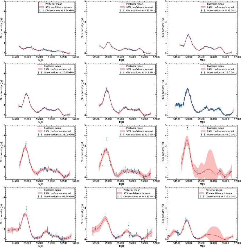
Figure 1: Gaussian process regression curves for the radio light curves in the range 2.64–226.50 GHz, shown here with the minimum flux density, $S_{0}$, subtracted. Observations are shown in blue, the posterior mean (prediction curve) in red, and the 95% confidence interval is the lighter red-shaded area.

Table 1: Results of the Gaussian process regression.

$\nu$	$S_{0}$	$S_{\rm m}$	$t_{\rm m}$	$t_{\rm r}$	$t_{\rm d}$
(GHz)	(Jy)	(Jy)	(MJD)	(d)	(d)
$2.64$	$0.868$	$0.593\pm 0.032$	$55095.2$	$239.9$	$366.8$
$4.85$	$0.777$	$1.084\pm 0.031$	$55016.8$	$201.8$	$383.2$
$8.35$	$0.740$	$1.764\pm 0.043$	$54980.4$	$230.9$	$435.9$
$10.45$	$0.725$	$2.055\pm 0.062$	$54968.7$	$234.9$	$435.0$
$14.60$	$0.683$	$2.414\pm 0.088$	$54954.4$	$288.1$	$467.6$
$15.00$	$0.711$	$2.570\pm 0.026$	$54952.3$	$276.2$	$391.7$
$23.05$	$0.478$	$2.856\pm 0.189$	$54921.9$	$390.8$	$457.0$
$32.00$	$0.516$	$2.590\pm 0.277$	$54916.7$	$447.9$	$446.5$
$43.05$	$0.299$	$3.542\pm 0.454$	$54925.8$	$383.4$	$527.2$
$86.24$	$0.507$	$2.439\pm 0.144$	$54912.8$	$331.3$	$437.2$
$142.33$	$0.263$	$1.987\pm 0.254$	$54888.0$	$313.5$	$444.5$
$226.50$	$0.238$	$1.823\pm 0.102$	$54914.3$	$300.3$	$460.8$

2.2 The discrete cross-correlation function

Putative correlated variability across observing bands, based on sampling-rate-limited time series, can be investigated and quantified using the discrete cross-correlation function (DCCF, Edelson & Krolik, 1988).

The cross-correlation function (CCF), as a function of the time lag $\tau$, for two discrete and evenly sampled light curves, $x(t_{i})$ and $y(t_{i})$, is given by

$${\rm CCF}(\tau)=\dfrac{1}{N}\sum_{i=1}^{N}\dfrac{\left[x(t_{i})-\bar{x}\right]\left[y(t_{i}-\tau)-\bar{y}\right]}{\sigma_{x}\sigma_{y}},$$ (6)

where

$$\begin{array}[]{lp{0.8\linewidth}}\bar{x}&is the mean value of the light curve $x(t_{i})$,\\ \sigma_{x}&its standard deviation,\\ \bar{y}&is the mean of the light curve $y(t_{i})$, and\\ \sigma_{y}&is the standard deviation of light curve $y(t_{i})$.\\ \end{array}$$

Uneven sampling of light curves introduces the need for the discrete cross-correlation function (Edelson & Krolik, 1988, see also Larsson, 2012; Robertson et al., 2015). Contrary to linear interpolation methods, the DCCF takes into consideration only the data points themselves. For two irregularly sampled light curves, the unbinned CCF (UCCF) is

$${\rm UCCF}_{ij}(\tau)=\dfrac{\left(x_{i}-\bar{x}\right)\left(y_{i}-\bar{y}\right)}{\sqrt{(\sigma_{x}^{2}-\bar{\varepsilon}_{x}^{2})(\sigma_{y}^{2}-\bar{\varepsilon}_{y}^{2})}},$$ (7)

where $\bar{\varepsilon}$ is the mean measurement uncertainty of each data set. For the calculation of the mean and standard deviation, only data within each time lag bin are considered. Averaging the UCCF over the number of data pairs, $M$, yields the DCCF $({\rm DCCF}=\frac{1}{M}\sum{\rm UDCF}_{ij}$) and an uncertainty associated with each time lag can be determined as

$$\sigma_{\rm DCCF}(\tau)=\dfrac{1}{M-1}\sqrt{\sum{\left[{\rm UDCF}_{ij}-{\rm DCCF}(\tau)\right]}^{2}}.$$ (8)

Positive DCCF values indicate a positive correlation with an average time shift $\tau$, while negative values imply anti-correlation.

Using the DCCF, Fuhrmann et al. (2014) searched for possible correlations between the 3 mm radio waveband and the Fermi $\gamma$-ray observations for the F-GAMMA blazar sample. Their study has shown the presence of significantly correlated 3 mm/$\gamma$-ray variability in an average sense (whole sample). Specifically, for PKS 1502+106 a 3 mm/$\gamma$-ray correlation is detected at a significance level above 99%, with the mm-radio emission lagging behind $\gamma$ rays by $14\pm 11$ days. The aforementioned difference in the time of arrival translates into a de-projected relative separation of the corresponding emitting regions of 2.1 pc, with the $\gamma$-ray active region upstream of the 3 mm (or 86.24 GHz) core.

Here, we enhance these findings and quantify the correlated variability beyond the mm/sub-mm band using all available radio observations (see Fig. 1 for the light curves). The DCCFs have been calculated between the 15 GHz light curve of the OVRO 40 m blazar monitoring program and all available light curves, from 226.5 down to 2.64 GHz. For each DCCF we employed a time lag bin width of 30 days within a window of $\pm 750$ d. The better sampling of the OVRO 15 GHz light curve led to its selection as reference. Hereafter, we refer to the cross-correlated light curves as the reference (OVRO 15 GHz) and the target (all the rest). A positive lag $\tau_{\rm DCCF}$ implies that the target waveband, lags behind the reference frequency by $\tau_{\rm DCCF}$, measured in days. We use a weighted Gaussian fit, of the form $G(x)=\alpha\,\exp\left[\frac{-(x-\mu)^{2}}{2\sigma^{2}}\right]$, to obtain the DCCF peak and its position. Since the value of interest is the peak of the DCCF, the Gaussian fit is performed in the time lag range that ensures better peak determination. The mean of the Gaussian is the value of time lag $\tau_{\rm DCCF}$ reported in Tab. 2. Left panels of Figs. 2 and 3 show all DCCFs with respect to our selected reference frequency along with the Gaussian fit.

For estimating the time-lag uncertainty we employ the model-independent Monte Carlo (MC) approach introduced by Peterson et al. (1998) (see also Raiteri et al., 2003). The two main sources of uncertainty in cross-correlation analyses – in addition to limited data trains and consequently limited number of events – are: (i) flux uncertainties and (ii) uncertainties associated with the uneven sampling of the light curves. The method comprises two parts; that of the flux redistribution (FR), and that of a random sample selection (RSS), accounting for (i) and (ii) respectively. The algorithm is essentially as follows:

1. Introduction of Gaussian deviates to the data, constrained by the maximum flux density uncertainty.

2. Use of a re-sampling with replacement scheme to randomly select data points and create an equally long light curve; i.e. a bootstrap-like procedure.

3. Calculation of the DCCF and determination of the time lag.

4. After a given number of MC realizations, obtain the cross-correlation peak distribution (CCPD).

The uncertainty, $\pm\Delta\tau_{68\%}$, or simply $\pm\Delta\tau$, is obtained directly from the CCPD and corresponds to the time lag interval of ($\tau_{\rm median}-\Delta\tau$) and ($\tau_{\rm median}+\Delta\tau$), such that $68\%$ of the realizations yield results within this interval. This estimate is equivalent to the $1\sigma$ error, in case of a Gaussian distribution (Peterson et al., 1998). Here, 5000 MC realizations were performed.

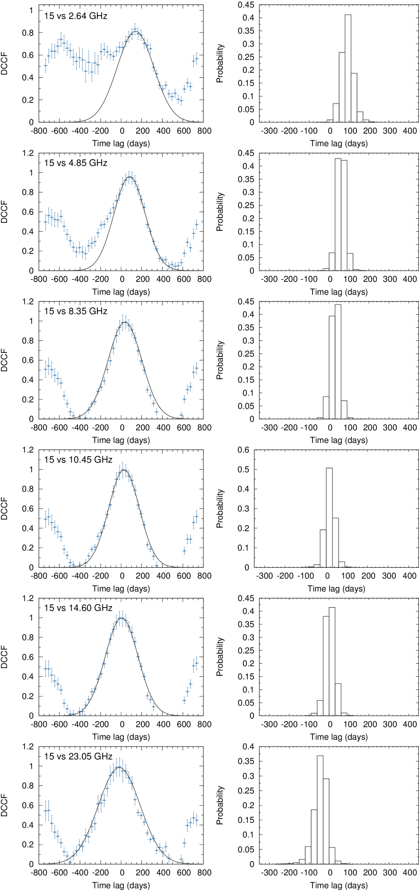
Figure 2: DCCFs between the 15 GHz light curve and those in the range 2.64 to 23.05 GHz. Solid lines represent the best-fit Gaussian functions.

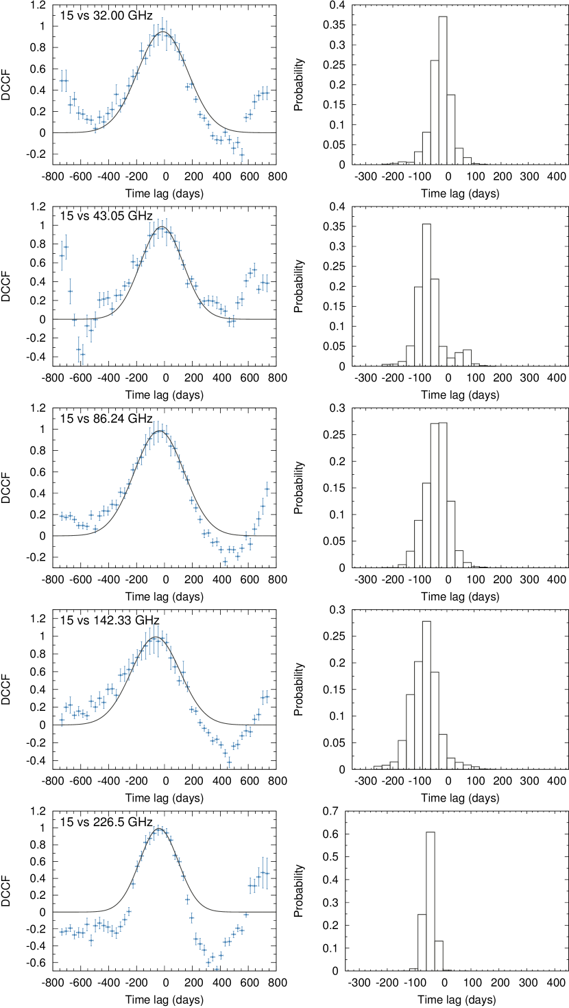
Figure 3: DCCFs between the 15 GHz light curve and those in the range 32.00 to 226.5 GHz. Solid lines represent the best-fit Gaussians.

Table 2: Results of the correlation analysis at all frequencies.

$\nu$	$\alpha$	$\mu$	$\sigma$
(GHz)		(d)	(d)
2.64	$0.81\pm 0.01$	$139.87\pm 8.15$	$178.05\pm 39.64$
4.85	$0.96\pm 0.01$	$82.12\pm 1.03$	$151.60\pm 2.37$
8.35	$0.99\pm 0.01$	$37.19\pm 1.98$	$164.54\pm 4.81$
10.45	$0.99\pm 0.01$	$28.11\pm 2.85$	$149.57\pm 7.61$
14.60	$1.00\pm 0.01$	$5.15\pm 1.05$	$159.42\pm 3.94$
23.05	$0.98\pm 0.01$	$-17.74\pm 3.48$	$204.18\pm 10.01$
32.00	$0.95\pm 0.01$	$-12.31\pm 3.24$	$179.45\pm 5.99$
43.05	$0.99\pm 0.01$	$-19.04\pm 5.38$	$152.45\pm 7.03$
86.24	$0.98\pm 0.01$	$-37.67\pm 4.34$	$178.78\pm 10.90$
142.33	$0.99\pm 0.02$	$-62.98\pm 5.88$	$175.25\pm 15.00$
226.50	$0.99\pm 0.02$	$-39.89\pm 4.84$	$138.46\pm 9.00$

3 Results

3.1 Flare parameters

The flare amplitudes, $S_{\rm m}$, show an increasing trend with frequency, up to about 43 GHz whereafter they start decaying again as seen for 86.24, 142.33, and 226.5 GHz (see Fig. 4). As will be discussed later, there exists a clear tendency for the flare to be visible earlier at higher frequencies, an effect attributed to synchrotron opacity (see also Fig. 5). The flare rising times, while initially increase with frequency, at frequencies higher than 32.00 GHz show a decreasing trend (see Tab. 1). Finally, in terms of the flare decay times they seem to be following a slightly increasing trend with observing frequency in the whole range employed here (Tab. 1).

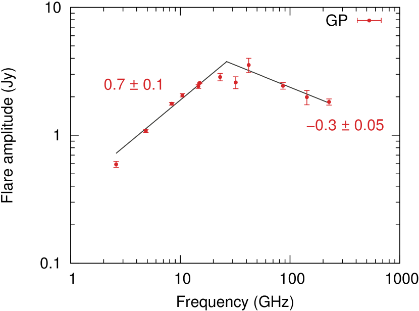
Figure 4: Frequency dependence of the flare amplitudes. Solid lines show the wings of the fitted broken power law, while the values denote their slopes.

3.2 Frequency-dependent time lags

The DCCFs shown in Figs. 2 and 3 confirm the presence of a correlation between the outburst seen across observing frequencies. Essentially in all cases, a single strong peak is clearly visible. In the following, we use the obtained time lag where the DCCF peaks (Tab. 2), referenced to the highest-frequency, well-sampled light curve at 142.33 GHz. The final $\tau_{\rm DCCF}$ are reported in Tab. 3.

In Fig. 5 the delays obtained with both methods are shown. The GP regression and the DCCF analysis yield conclusive results that agree very well. A systematic trend is clearly seen, in the sense that the time lags become larger towards lower frequencies. This trend is described well by a power-law. In order to obtain its index, the frequency-dependent delays are fitted by a power-law of the form $a\nu^{-1/k_{\rm r}}$ using a least-squares procedure. The results for index $k_{\rm r}$ are for the GP regression $k_{\rm r,\,GP}=(1.4\pm 0.1)$ and $k_{\rm r,\,DCCF}=(1.6\pm 0.1)$ for the DCCF results. Both are shown, along with the best-fit curves, in Fig. 5.

The rather conservative uncertainty estimates of the FR/RSS method (Peterson et al., 1998) and the good agreement between $\tau_{\rm DCCF}$ and $\tau_{\rm GP}$ allow an average time lag, $\left<\tau\right>$, and its standard error to be obtained (Tab. 3). Hereafter, this average value is used for all calculations and all uncertainties are formally propagated. The longest delay of $(205\pm 2.0)$ days is seen between $142.33$ and $2.64$ GHz. A decreasing trend is clearly visible towards higher frequencies with a time lag of $(136.9\pm 8.1)$ d at 4.85 GHz and $\left<\tau\right>=(96.2\pm 3.8)$ d at 8.35 GHz. Between the two highest frequencies of 142.33 GHz and 86.24 GHz, it is $\left<\tau\right>=(24.8\pm 0.2)$ days (see Tab. 3).

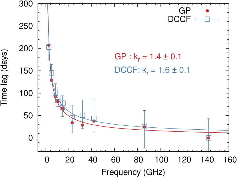
Figure 5: Frequency dependence of the time lags with respect to the data at 142.33 GHz. Red circles denote values resulting from the GP regression and blue squares those from the DCCF analysis. Solid lines represent the best-fit power laws.

Table 3: Frequency-dependent time lags and “time-lag core shifts” with respect to the observations at $142.33$ GHz.

$\nu$	$\tau_{\rm GP}$	$\tau_{\rm DCCF}$	$\left<\tau\right>$	$\Delta r$	$\Omega_{{\rm r}\nu}$
(GHz)	(d)	(d)	(d)	(mas)	(pc GHz)
$2.64$	$207.1$	$203\,^{+29}_{-29}$	$205.0\pm 2.0$	$0.051\pm 0.005$	$0.885\pm 0.093$
$4.85$	$128.8$	$145\,^{+19}_{-20}$	$136.9\pm 8.1$	$0.034\pm 0.004$	$0.922\pm 0.118$
$8.35$	$92.4$	$100\,^{+21}_{-22}$	$96.2\pm 3.8$	$0.024\pm 0.003$	$0.981\pm 0.127$
$10.45$	$80.6$	$91\,^{+23}_{-21}$	$85.8\pm 5.2$	$0.021\pm 0.002$	$1.046\pm 0.148$
$14.60$	$66.3$	$68\,^{+26}_{-20}$	$67.2\pm 0.9$	$0.017\pm 0.002$	$1.081\pm 0.147$
$15.00$	$64.2$	$63\,^{+43}_{-51}$	$63.6\pm 0.6$	$0.016\pm 0.002$	$1.047\pm 0.142$
$23.05$	$33.8$	$45\,^{+28}_{-34}$	$39.4\pm 5.6$	$0.010\pm 0.002$	$0.955\pm 0.194$
$32.00$	$28.6$	$51\,^{+34}_{-30}$	$39.8\pm 11.2$	$0.010\pm 0.003$	$1.338\pm 0.428$
$43.05$	$37.7$	$44\,^{+41}_{-31}$	$40.8\pm 3.1$	$0.010\pm 0.001$	$1.915\pm 0.339$
$86.24$	$24.7$	$25\,^{+36}_{-48}$	$24.8\pm 0.2$	$0.006\pm 0.001$	$3.585\pm 0.623$

3.3 Time-lag core shifts and synchrotron opacity structure

Like most blazars, PKS 1502+106 features a flat-spectrum core, indicative of the superposition of optically thick synchrotron components (e.g. Kaiser, 2006). In addition to the scenario that the observed VLBI core is the first stationary hotspot (recollimation shock) of the jet (Daly & Marscher, 1988; Gómez et al., 1995), a widely accepted interpretation is that this core is the point of the continuous flow where the photons at a given frequency have sufficient energy to escape the opacity barrier. Within this scenario, the core is the surface where the optical depth is close to unity at a given frequency (e.g. Königl, 1981). The standard relativistic jet paradigm (Blandford & Königl, 1979; Königl, 1981) predicts that the apparent position of this unit-opacity surface depends on observing frequency. Therefore, according to the interpretation of the VLBI core discussed above, its position must also be frequency-dependent. This “core-shift effect” was first observed by Marcaide & Shapiro (1984) and ever since has been studied using multi-frequency VLBI (e.g. Lobanov, 1998; Kovalev et al., 2008; Sokolovsky et al., 2011; Pushkarev et al., 2012). The importance of core-shift measurements lies in the fact that they can provide critical insights into the structure and physics of ultracompact jets, such as the position of the core at each frequency relative to the jet base, and the magnetic field in different locations along the relativistic flow (e.g. Lobanov, 1998; Hirotani, 2005).

Relative timing of total flux density outbursts, as seen in single-dish radio observations, presents a viable alternative to VLBI core shifts. Let us return back to the standard jet model. Here, a disturbance originating at the jet base will propagate outwards along the jet. As this disturbance or shock moves away from the base it crosses the sequence of physically separated regions where the jet flow becomes optically thin – i.e. the VLBI cores – as seen at a given sequence of observing frequencies. When the disturbance reaches a given unit-opacity surface for a given frequency $\nu_{\rm i}$, the synchrotron flare emission most likely becomes optically thin at $\nu_{\rm i}$. This appears in single-dish light curves as a total intensity outburst, while in VLBI maps these travelling shocks manifest as regions of enhanced emission after the core, the so-called VLBI knots (Marscher & Gear, 1985). Since the times of maxima in single-dish light curves correspond to the flare emission becoming optically thin at the unit-opacity surface, for a given frequency, it follows that these times are frequency-dependent as well, and carry information on the opacity of each core. In other words, through relative timing of the same flaring event seen at different bands, we can obtain a tomography of the jet in terms of nuclear opacity, similar to VLBI core-shift measurements (e.g. Kudryavtseva et al., 2011; Kutkin et al., 2014).

An important consideration to be taken into account is that the method is based on the absence of any optically thick component downstream of the core. If there was any, it would sooner or later induce an opacity-driven enhancement of flux density due to its expansion and subsequent drop of density at a region further away from the core, the position of which we try to constrain. Essentially, the emission needs to become optically thin when it reaches each respective unit-opacity surface. In this respect and given the spectra of VLBI components presented in Karamanavis et al. (2016), component C3, which is used for our calculations, is optically thin at least between 43 and 86 GHz (spectral index $\alpha_{\rm 43/86\,GHz}=-0.8\pm 0.3$).

Based on Lobanov (1998), a “time-lag core-shift” between two frequencies $\nu_{1}$ and $\nu_{2}$, with $\nu_{2}$ ¿ $\nu_{1}$, can be defined as follows (see also Kudryavtseva et al., 2011)

$$\Omega_{{\rm r}\nu}=4.85\times 10^{-9}\dfrac{\mu\,\Delta t\,\rm{D_{L}}}{(1+z)^{2}}\left(\dfrac{\nu_{1}^{1/k_{\rm r}}\cdot\nu_{2}^{1/k_{\rm r}}}{\nu_{2}^{1/k_{\rm r}}-\nu_{1}^{1/k_{\rm r}}}\right),$$ (9)

in units of pc GHz for $k_{r}=1$, where

$$\begin{array}[]{lp{0.8\linewidth}}\mu&is the VLBI jet proper motion in mas\,yr${}^{-1}$,\\ \Delta t&is the observed time lag between the frequency pair $\nu_{1}$ and $\nu_{2}$ in yr,\\ \rm{D_{L}}&is the luminosity distance in pc,\\ z&is the redshift,\\ \nu_{1},\nu_{2}&are the first and second observing frequency, both expressed in GHz, and\\ k_{\rm r}&is the power-law index obtained by fitting the cross-band delays.\end{array}$$

Here, $k_{\rm r}=[(3-2\alpha)m+2n-2]/(5-2\alpha)$ with $m$ and $n$ denoting the index of the power-law dependence of the magnetic field $B(r)\propto r^{-m}$ and the electron number density $N_{\rm e}(r)\propto r^{-n}$, at distance $r$ along the jet, respectively. Finally, $\alpha$ denotes the optically thin spectral index. In case of external density gradients and/or free-free absorption, it is $k_{\rm r}>1$. For synchrotron self-absorption (SSA) dominated opacity and equipartition between particle energy and magnetic field energy, $k_{\rm r}=1$ for $m=1$ and $n=2$ independently of $\alpha$. The angular offset in units of mas is given by $\Delta r=\mu\left<\tau\right>$. That is, the distance traveled by the disturbance within the time interval $\left<\tau\right>$ (Tab. 3). Using $\Omega_{{\rm r}\nu}$ and following Lobanov (1998), Hirotani (2005), and Kudryavtseva et al. (2011) we obtain the distance between the core and the base of the assumed-conical jet. The frequency-dependent distance of the core – at any frequency $\nu$ – is given by

$$r_{\rm core}(\nu)=\dfrac{\Omega_{{\rm r}\nu}}{\sin\theta}\nu^{-1/k_{\rm r}}.$$ (10)

We employ Eqs. 9 and 10 to infer the separation of the radio core at each frequency from the jet base. In that, we use the average $k_{\rm r}=(1.5\pm 0.1)$ calculated based on the DCCF analysis and the Gaussian process regression. Both agree very well with each other indicating that $k_{\rm r}>1$. This implies the possible presence of jet external density gradients and/or foreground free-free absorption. Other parameters used are $\mu=0.09$ mas yr^-1 which corresponds the proper motion of component C3 at 86 GHz, responsible for the flare, and $\theta=2.6^{\circ}$ the critical viewing angle (Karamanavis et al., 2016).

Our results reveal the nuclear opacity structure of PKS 1502+106 (see Tab. 4). The largest distance of about 10 pc is seen for the 2.64 GHz core, as expected, and distances diminish as we go towards higher frequencies. At observing frequencies between 23.05 and 43.05 GHz the light curves become slightly more sparsely sampled due to the fact that weather effects and poorer system performance of the Effelsberg 100-m telescope, at those bands, play an increasingly important role. At the highest frequency of 86.24 GHz, the core lies at a distance of $(4.0\pm 1.1)$ pc away from the jet base.

Table 4: Synchrotron opacity structure and magnetic field tomography of the jet of PKS 1502+106.

$\nu$	$r_{\rm core}$	$B_{1\,{\rm pc}}\leavevmode\nobreak\ \leavevmode\nobreak\ [B_{1\,{\rm pc\,min}},B_{1\,{\rm pc\,max}}]$	$B_{\rm core}\leavevmode\nobreak\ \leavevmode\nobreak\ [B_{\rm core\,min},B_{\rm core\,max}]$
(GHz)	(pc)	(mG)	(mG)
2.64	$10.2\pm 1.2$	$148\leavevmode\nobreak\ \leavevmode\nobreak\ \leavevmode\nobreak\ \leavevmode\nobreak\ [106,209]$	$\leavevmode\nobreak\ \leavevmode\nobreak\ 14\leavevmode\nobreak\ \leavevmode\nobreak\ \leavevmode\nobreak\ \leavevmode\nobreak\ \leavevmode\nobreak\ \leavevmode\nobreak\ [11,20]$
4.85	$7.1\pm 1.0$	$154\leavevmode\nobreak\ \leavevmode\nobreak\ \leavevmode\nobreak\ \leavevmode\nobreak\ [111,220]$	$\leavevmode\nobreak\ \leavevmode\nobreak\ 22\leavevmode\nobreak\ \leavevmode\nobreak\ \leavevmode\nobreak\ \leavevmode\nobreak\ \leavevmode\nobreak\ \leavevmode\nobreak\ [16,30]$
8.35	$5.3\pm 0.8$	$166\leavevmode\nobreak\ \leavevmode\nobreak\ \leavevmode\nobreak\ \leavevmode\nobreak\ [121,233]$	$\leavevmode\nobreak\ \leavevmode\nobreak\ 32\leavevmode\nobreak\ \leavevmode\nobreak\ \leavevmode\nobreak\ \leavevmode\nobreak\ \leavevmode\nobreak\ \leavevmode\nobreak\ [24,43]$
10.45	$4.8\pm 0.8$	$178\leavevmode\nobreak\ \leavevmode\nobreak\ \leavevmode\nobreak\ \leavevmode\nobreak\ [129,253]$	$\leavevmode\nobreak\ \leavevmode\nobreak\ 37\leavevmode\nobreak\ \leavevmode\nobreak\ \leavevmode\nobreak\ \leavevmode\nobreak\ \leavevmode\nobreak\ \leavevmode\nobreak\ [27,51]$
14.60	$4.0\pm 0.7$	$185\leavevmode\nobreak\ \leavevmode\nobreak\ \leavevmode\nobreak\ \leavevmode\nobreak\ [137,259]$	$\leavevmode\nobreak\ \leavevmode\nobreak\ 46\leavevmode\nobreak\ \leavevmode\nobreak\ \leavevmode\nobreak\ \leavevmode\nobreak\ \leavevmode\nobreak\ \leavevmode\nobreak\ [35,63]$
15.00	$3.8\pm 0.7$	$178\leavevmode\nobreak\ \leavevmode\nobreak\ \leavevmode\nobreak\ \leavevmode\nobreak\ [132,249]$	$\leavevmode\nobreak\ \leavevmode\nobreak\ 47\leavevmode\nobreak\ \leavevmode\nobreak\ \leavevmode\nobreak\ \leavevmode\nobreak\ \leavevmode\nobreak\ \leavevmode\nobreak\ [36,64]$
23.05	$2.6\pm 0.6$	$161\leavevmode\nobreak\ \leavevmode\nobreak\ \leavevmode\nobreak\ \leavevmode\nobreak\ [113,237]$	$\leavevmode\nobreak\ \leavevmode\nobreak\ 62\leavevmode\nobreak\ \leavevmode\nobreak\ \leavevmode\nobreak\ \leavevmode\nobreak\ \leavevmode\nobreak\ \leavevmode\nobreak\ [45,88]$
32.00	$2.9\pm 1.0$	$235\leavevmode\nobreak\ \leavevmode\nobreak\ \leavevmode\nobreak\ \leavevmode\nobreak\ [142,398]$	$\leavevmode\nobreak\ \leavevmode\nobreak\ 80\leavevmode\nobreak\ \leavevmode\nobreak\ \leavevmode\nobreak\ \leavevmode\nobreak\ [51,131]$
43.05	$3.4\pm 0.8$	$352\leavevmode\nobreak\ \leavevmode\nobreak\ \leavevmode\nobreak\ \leavevmode\nobreak\ [249,522]$	$102\leavevmode\nobreak\ \leavevmode\nobreak\ \leavevmode\nobreak\ \leavevmode\nobreak\ [76,145]$
86.24	$4.0\pm 1.1$	$711\leavevmode\nobreak\ \leavevmode\nobreak\ [494,1086]$	$176\leavevmode\nobreak\ \leavevmode\nobreak\ [129,254]$

3.4 Equipartition magnetic field

We obtain an expression for the magnetic field at 1 pc from the jet base, $B_{1\,{\rm pc}}$, by evaluating Eq. (43) of Hirotani (2005) (see also O’Sullivan & Gabuzda, 2009; Kutkin et al., 2014). Under equipartition between the energies of the magnetic field and that of radiating particles, and with a spectral index $\alpha=-0.5$, this yields

$$B_{1\,{\rm pc}}\approx 0.014\leavevmode\nobreak\ \left[\dfrac{\Omega_{{\rm r}\nu}^{3k_{\rm r}}\,(1+z)^{2}\ln(\gamma_{\rm max}/\gamma_{\rm min})}{\delta^{2}\phi\sin^{3k_{\rm r}-1}\theta}\right]^{1/4}\leavevmode\nobreak\ \leavevmode\nobreak\ \leavevmode\nobreak\ \leavevmode\nobreak\ \leavevmode\nobreak\ ({\rm G}),$$ (11)

where

$$\begin{array}[]{lp{0.75\linewidth}}\gamma_{\rm max},\gamma_{\rm min}&are the maximum and minimum Lorentz factors of the emitting $e^{-}$,\\ \delta&is Doppler factor,\\ \phi&is the half-opening angle of the jet, and\\ \theta&is the viewing angle.\end{array}$$

Then, the magnetic field strength at the core is given by

$$B_{\rm core}(\nu)=B_{1\,{\rm pc}}\,r_{\rm core}(\nu)^{-1}.$$ (12)

We adopt $\ln(\gamma_{\rm max}/\gamma_{\rm min})=10$ and employ the values for the Doppler factor and half-opening angle, deduced in Karamanavis et al. (2016), of $\delta=10$ and $\phi=(1.90\pm 0.25)^{\circ}$, respectively corresponding to components travelling within the inner jet of PKS 1502+106. Resulting values for $B_{1\,{\rm pc}}$ and $B_{\rm core}$ are summarized in Tab. 4. Here, we also report a conservative range for these values, by combining the uncertainties of the input parameters in a way that maximizes this range. Inferred magnetic field strengths are higher at higher frequencies, when approaching the jet base. The values range between 14 and 176 mG for the 2.64 GHz (outermost) and 86.24 GHz (innermost) cores, respectively.

The results presented here are in reasonable agreement with the core shift measurements of PKS 1502+106 derived by Pushkarev et al. (2012) who employ standard VLBI techniques and obtain a separation of ${\sim}8$ pc between the 15 GHz VLBI core and the vertex of the jet. Some discrepancies can be seen in the – inferred from VLBI core shifts – physical parameters of the jet, such as the magnetic field at a distance of 1 pc and in the 15 GHz core ($B_{1\,{\rm pc}}$ and $B_{\rm core}$), but these can be explained through the different kinematical parameters used. Specifically, Pushkarev et al. (2012) make use of the fastest non-accelerating, component’s apparent speed from data covering the period 1994 August to 2007 September, as reported in Lister et al. (2009). However, here we use the proper motion, $\mu$, of the knot most likely responsible for the multi-wavelength flare of 2008/2010 (knot C3 in Karamanavis et al., 2016) whose apparent angular velocity – while travelling in the inner jet of PKS 1502+106 – is about half of what Pushkarev et al. (2012) use.

4 Discussion

4.1 Localizing the $\gamma$-ray emission

Our ultimate goal of pinpointing the $\gamma$-ray emission region is reached by combining the findings of the present study with those of Fuhrmann et al. (2014), who deduce a relative distance between the $\gamma$-ray active region and the 86.24 GHz unit-opacity surface of about 2.1 pc (cf. Ramakrishnan et al., 2015). Here, based on the opacity-driven time lags across the eleven observing frequencies, the distance of the 86.24 GHz core from the jet base is $(4.0\pm 1.1)$ pc. From the combination follows that the $\gamma$-ray emission region is best constrained to a distance of $(1.9\pm 1.1)$ pc away from the jet base. In a similar study, Max-Moerbeck et al. (2014) obtain a time lag of $(-40\pm 13)$ d between the leading $\gamma$-rays and the lagging 15 GHz radio emission. Following their argumentation, this time lag translates into a relative distance of $(2\pm 1)$ pc between the 15 GHz unit-opacity surface and the $\gamma$-ray site. Combining our $r_{\rm core}$ at 15 GHz (Tab. 4) with the aforementioned value, we obtain a separation of $(1.8\pm 1.2)$ pc between the jet base and the $\gamma$-ray active region, comparable with our previous result based on the 86.24 GHz time lag. We reiterate that in the present work we use the VLBI kinematical parameters of the knot connected to the 2008/10 flare of PKS 1502+106 (C3, see Sect. 3.4). Finally, our results are in agreement with the upper limit of ${\leq}5.9$ pc reported by Karamanavis et al. (2016), based on mm-VLBI imaging.

At $(1.9\pm 1.1)$ pc from the jet base, the high-energy emission originates well beyond the bulk of the BLR material of PKS 1502+106, placed at ${\rm R}_{\rm BLR}\approx 0.1$ pc (Abdo et al., 2010). A $\gamma$-ray emission region placed so far away from the BLR almost negates the notion that BLR photons alone can be used as the target photon field for inverse Compton up-scattering to $\gamma$-rays, thus other or additional seed photon fields (e.g. torus, synchrotron self-Compton, SSC) need to be involved in the process.

4.2 A shock origin for the 2008/10 flare

Overall, the slopes extracted from the multi-wavelength light curves agree well with the expectations of the shock-in-jet model (Marscher & Gear, 1985), indicating a shock origin for the 2008/2010 flare of PKS 1502+106. In the following, the observed light curve parameters (flare amplitudes and cross-band delays) are discussed in conjunction with the results of analytical shock-in-jet model simulations (Fromm et al., 2015). The frequency dependence of flare amplitudes is shown in Fig. 4 and of the cross-frequency delays in Fig. 5. Flare amplitudes rise with frequency until they culminate at a frequency of about 43 GHz, after which the amplitude of the flare drops. The rise and decay wings follow a trend that is described well by a broken power law, in very good agreement with the shock model expectations. The slopes are $\epsilon_{\rm flare\,amp\,rise}=(0.7\pm 0.1)$ for the rising part of the flare amplitude and $\epsilon_{\rm flare\,amp\,decay}=(-0.3\pm 0.05)$ for the decaying part. The power-law slope of the observed time lags, $\epsilon_{\rm time-lag}=-1/k_{\rm r}$ (see Sect. 3) is $\epsilon_{\rm time-lag}\approx-0.7$ (see Fig. 5). This value is obtained by averaging over the two values arising from the GP regression and the DCCF analysis and is in accord with the pattern expected from the shock model. By comparing the slope of the frequency-dependent cross-band delays with the finding of Fromm et al. (2015), we can safely exclude the scenario of a decelerating jet. Our findings in fact suggest the presence of a certain degree of acceleration taking place within the relativistic jet of PKS 1502+106.

5 Conclusions

In the present work we exploited the dense, long-term F-GAMMA radio light curves in the frequency range 2.64–142.33 GHz obtained with the Effelsberg 100-m and IRAM 30-m telescopes. The F-GAMMA data were complemented by light curves at 15.00 GHz (OVRO) and 226.5 GHz (SMA).

A detailed section was devoted to the two independent approaches used in order to quantify the observed flare of PKS 1502+106 in the time domain. These are: (i) a Gaussian process regression and (ii) a discrete cross-correlation function analysis. This is the first time that GP regression is used in the field of blazar variability and it has shown to perform well. It is a viable approach to the problem of modelling discrete, unevenly sampled, blazar light curves and extracting the relevant parameters.

The flare in PKS 1502+106 is a “clean”, isolated outburst seen across observing frequencies. Our findings suggest a frequency-dependence for the cross-band delays and the flare amplitudes. The flare amplitudes first increase – up to the frequency of ${\sim}43$ GHz, where they peak – after which a decreasing trend follows (Fig. 4). The times at which the flare peaks are characterized by increasing time delay towards lower frequencies (Fig. 5). The characteristic dependence of these parameters on the observing frequency can be approximated by power laws, indicative of shock evolution and pc-scale jet acceleration.

Through the observed opacity-driven time lags, the structure of PKS 1502+106 in terms of synchrotron opacity is deduced – i.e. using a “time-lag core shift” method. The positions of the ten radio unit-opacity surfaces with respect to the jet base were deduced, with distances in the range $(10.2\pm 1.2)$ pc to $(4.1\pm 1.1)$ pc for the core between 2.64 and 86.24 GHz, respectively.

The frequency-dependent core positions also enable a tomography of the magnetic field along the jet axis. We obtain the equipartition magnetic field at the position of each core, $B_{\rm core}$, and also at a distance of 1 pc from the jet base, $B_{1\,{\rm pc}}$. The former, between the 2.64 and 86.24 GHz unit-opacity surfaces, are in the range $B_{\rm core,\,2.64}\sim 14$ mG and $B_{\rm core,\,86.24}\sim 176$ mG. For the latter, our figures indicate an average value of $\left<B_{1\,{\rm pc}}\right>=(174\pm 55)$ mG.

The $\gamma$-ray emission region is constrained to $(1.9\pm 1.1)$ pc away from the jet base, well beyond the bulk of the BLR material of PKS 1502+106. This yields a contribution of IR torus photons and/or SSC to the production of $\gamma$ rays in PKS 1502+106, while almost negates the contribution of accretion disk or BLR photons alone.

The flare complies with the typical shock evolutionary path and its overall behavior in the time domain is in accord with the shock-in-jet scenario. When seen in the light of the VLBI findings discussed in Karamanavis et al. (2016), our results corroborate the scenario that the flare of PKS 1502+106 was induced by a shock, seen in mm-VLBI images as component C3, travelling downstream of the core at 43/86 GHz maps. This travelling disturbance is associated with the multi-frequency flare seen from radio up to $\gamma$-ray energies.