Equatorial superrotation in Held & Suarez-like flows
with weak equator-to-pole surface temperature gradient

Abstract

Equatorial superrotation under zonally-symmetric thermal forcing is investigated in a setup close to that of the classic Held and Suarez (1994) setup. In contrast to the behaviour in the classic setup, a transition to equatorial superrotation occurs when the equator-to-pole surface equilibrium entropy gradient is weakened. Two factors contribute to this transition: 1) the reduction of breaking Rossby waves from the mid-latitude that decelerate the equatorial flow and 2) the presence of barotropic instability in the equatorial region, providing stirring to accelerate the equatorial flow. In the latter, Kelvin waves excited by instability near the equator generate and maintain the superrotation. However, the superrotation is unphysically enhanced if simulations are under-resolved and/or over-dissipated.

1 Introduction

Superrotation is an important phenomenon in atmospheric flows. It is defined as a zonal-mean zonal flow with axial angular momentum, $M=M(\phi)$, greater than the solid body angular momentum at the equator, $M_{0}=M(0)$; here $\phi$ is the latitude. For a “shallow” atmosphere, $M=a\cos\phi(U+\Omega a\cos\phi)$ and therefore $M_{0}=\Omega a^{2}$, where $a$ is the planetary radius, $U$ is the zonal-mean zonal flow and $\Omega$ is the planetary rotation rate. Because superrotation away from the equator is inertially unstable, it is mainly manifested as prograde (westerly) flow at the equator. If friction maintains a solid body rotation at the surface (i.e., $M=M_{0}\cos^{2}\phi$ at the surface), a zonally-symmetric mean meridional circulation conserves $M$ such that $M\leq M_{0}$ at all latitudes in the absence of sources and sinks. In general, superrotation can be generated if there is a process which provides a steady eddy angular momentum flux directed up the meridional gradient of the angular momentum, $a^{-1}\partial M_{\phi}/\partial\phi$ (Hide, 1969, and see also Read 1986).

Superrotation is observed in the Earth’s atmosphere (e.g. the quasi-biennial oscillation), but it is only transient. The current explanation for the transience is that Rossby waves generated by baroclinic instability at mid-latitudes propagate upwards, then refract equatorward and break in the equatorial region (e.g. Held and Hoskins, 1985). Because the waves deposit prograde momentum in the source region and retrograde momentum in the breaking or saturation region, equatorial superrotation does not occur. On the other hand, superrotation does occur more robustly on other planets and in idealized general circulation model (GCM) experiments. For example, in the latter, superrotation occurs under a variety of forcing conditions: zonally-asymmetric tropical heating (e.g. Suarez and Duffy, 1992; Saravanan, 1993; Hoskins et al., 1999; Arnold et al., 2012), zonally-symmetric heating with a convective equatorial wave source (e.g. Schneider and Liu, 2009; Laraia and Schneider, 2015), and statically-stable zonally-symmetric heating with $\Omega$ or $a$ smaller than those of the Earth (e.g. Williams, 1988, 2003; Mitchell and Vallis, 2010). In the statically-stable zonally-symmetric case, the increase in the global scale Rossby number — effected by reducing $\Omega$ or $a$ — results in a weakened mid-latitude baroclinic instability and a strengthened barotropic instability. Williams (2003) and Mitchell and Vallis (2010) have attributed superrotation to barotropic instability.

Williams (2003) has also shown that superrotation can occur on a planet with Earth’s $\Omega$ and $a$ subject to statically-stable zonally-symmetric heating, when the center of maximum baroclinicity is shifted to a lower latitude than that in the classic setup of Held and Suarez (1994) [hereafter HS]. The shift is effected by narrowing the meridional width of the radiative heating profile compared to that in HS. In this case the barotropic instability at the equatorward flank of the subtropical jet provides the mechanism for producing superrotation. Williams (2006) has extended this work by showing that high tropospheric static stability enhances superrotation by inhibiting baroclinic instability.

Recently the barotropic instability view has been questioned by Potter et al. (2014). They propose that equatorial Kelvin waves drive and maintain superrotation in small $\Omega$ or $a$ flows and in Williams (2003), although the origin and precise driving mechanism of the Kelvin waves were not identified in their study. Later, Wang and Mitchell (2014) attribute the Kelvin waves to a linear resonant coupling of equatorial Kelvin and higher-latitude Rossby waves originating from an ageostrophic instability (e.g. Sakai, 1989): the instability ‘funnels’ westerly momentum to the equator, producing superrotation. However, as we shall show, in our study the superrotation is likely generated and maintained by different mechanisms.

Our study can be regarded as an extension of Williams (2003, 2006), Mitchell and Vallis (2010), Potter et al. (2014) and Wang and Mitchell (2014). Here transition to superrotation is also investigated under statically-stable zonally-symmetric thermal forcing; however, it is shown that superrotation also occurs with Earth’s $\Omega$ and $a$, if the equator-to-pole equilibrium temperature gradient near the surface (from 1000 hPa to 700 hPa) is weakened, compared to that in HS. While such a setup is not necessarily more (or less) realistic, it does help to elucidate the processes involved in producing superrotation. We show that when the temperature gradient is weak, baroclinic instability is weakened and barotropic instability in the equatorial region excites Kelvin waves, which help to drive superrotation. The key ingredient in the excitation is the stirring provided by the instability that occurs within the equatorial deformation length scale of a Kelvin wave. Further, we show that the strength of the resulting superrotation is strongly affected by numerical resolution and dissipation: superrotation is artificially strengthened by explicit and implicit model diffusion.

Throughout this paper, the reduced temperature gradient region is denoted as the ‘RTG’ region. Such a reduced gradient region is not necessarily meant to address the present-day Earth, but it may be relevant for past and future climates of the Earth or other ‘Earth-like’ planets in the Solar and extrasolar systems. For example, such a thermal forcing can be applicable to the runaway greenhouse state of paleo-Earth or the present-day atmosphere of Venus, both of which are characterized by a weak equator-to-pole surface temperature gradient (see e.g. Tziperman and Farrell, 2009; Yamamoto and Takanashi, 2003; Lee et al., 2005).

The overall plan of the paper is as follows. In section 2 the primitive equation model and the setup used in this study is discussed. In section 3 results from the model simulations with a RTG region are presented and compared with the classic HS-like simulations. This section also discusses in detail the non-convergence of simulations when they are under-resolved or over-dissipated. Finally, conclusions are given in section 4.

2 Method

2.1 Numerical model

In this study a global pseudospectral model, BOB (Scott et al., 2003), is used. BOB solves the ‘dry’ hydrostatic primitive equations in pressure ($p$) coordinates with rigid boundary conditions at the top and bottom of the model domain. The equations are solved in vorticity-divergence form. A parallel pseudospectral algorithm is used in the horizontal direction and a second-order finite differencing is used in the vertical direction. A hyperviscosity operator $-\nu\nabla^{8}$, with constant $\nu$, is applied to the prognostic variables (relative vorticity $\zeta$, divergence $\delta$ and potential temperature $\theta$). The timestepping is performed using a semi-implicit, second-order leapfrog scheme and the Robert-Asselin filter (Robert, 1966; Asselin, 1972) with a small filter coefficient ($=\!0.02$) is applied at each timestep to stabilize the time integration.

The physical setup is essentially that of HS, as well as Williams (2003) (his case $A$). A simple Newtonian relaxation scheme for the net heating,

$${\cal{Q}}=-\frac{1}{\tau}\Big{(}\theta-\theta_{\text{e}}\Big{)},$$ (1)

is applied in the potential temperature tendency equation; here $\tau$ is the characteristic relaxation time, and $\theta_{\text{e}}=\theta_{\text{e}}(\phi,p)$ is a specified equilibrium potential temperature distribution. The surface friction is parametrized as a linear, Rayleigh drag in the momentum equation:

$${\cal{D}}\ =\ -\frac{{\bf v}}{\tau_{\text{\tiny R}}}\ \max\!\left\{0,\,\frac{p-p_{\text{b}}}{p_{\text{s}}-p_{\text{b}}}\right\},$$ (2)

where ${\bf v}$ is the flow on an isobaric surface, $\tau_{\text{\tiny R}}$ is the characteristic damping time and $p_{\text{b}}$ and $p_{\text{s}}$ are the pressures at the top of the boundary layer (700 hPa) and at the bottom surface (1000 hPa), respectively. The only important physical difference relevant for superrotation in this setup, compared to that of HS, is $\theta_{\text{e}}$. This is discussed more in detail below.

Table 1: Parameter values used in the simulations: $g$ is the surface gravity; $a$ is the radius; $\Omega$ is the rotation rate; ${\cal R}$ is the gas constant; $c_{p}$ is the specific heat at constant pressure; $p_{\text{s}}$ is the surface pressure; $p_{\text{b}}$ is the top of the boundary layer pressure; $\tau$ is the radiative relaxation time; $\tau_{\text{\tiny R}}$ is the Rayleigh drag time; $T_{\text{s}}$ and $T_{0}$ are the stratospheric and upper tropospheric reference temperatures, respectively; $\Delta T$ is the equator-to-pole temperature difference; and, $\Delta\theta$ is the vertical potential temperature difference.

Parameter	Value	Units
$g$	9.8	m s-2
$a$	$6.4\!\times\!10^{6}$	m
$\Omega$	$7.3\!\times\!10^{-5}$	s-1
${\cal R}$	$287$	J kg-1 K-1
$c_{p}$	$1004$	J kg-1 K-1
$p_{\text{s}}$	$1000$	hPa
$p_{\text{b}}$	$700$	hPa
$\tau$	$20$	days
$\tau_{\text{R}}$	$1$	day
$T_{\text{s}}$	$200$	K
$T_{0}$	$255$	K
$\Delta T$	$60$	K
$\Delta\theta$	$10$	K

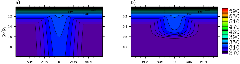
Figure 1: Prescribed zonally-symmetric radiative equilibrium potential temperature distribution $\theta_{\text{e}}$ [K], normalized pressure vs. latitude, for the control (HS-like) case ($a$) and the reduced temperature gradient (RTG) case ($b$). The contour interval is 10 K.

2.2 Setup

The physical parameters used in all the simulations discussed in this study are listed in Table 1. The simulations are initialized with an isothermal state of rest, with a small amount of Gaussian white noise ($10^{-7}$ s^-1 standard deviation) introduced to the $\zeta$ field to break symmetry. The specified equilibrium potential temperature is

$$\theta_{\text{e}}(p,\phi)=\text{max}\Biggl{\{}T_{\text{s}}\left(\frac{p_{\text{s}}}{p}\right)^{\kappa},\Bigl{[}T_{0}+\Delta T\,\cos^{b}\!\phi~{}F(p)$$

$$-\Delta\theta\,\log\left(\frac{p}{p_{s}}\right)\cos^{2}\!\phi\Bigr{]}\Biggr{\}}\,.$$ (3)

Here $T_{\text{s}}$ and $T_{0}$ are the stratospheric and upper tropospheric reference temperatures, respectively; $\Delta T$ is the equator-to-pole temperature difference; $\Delta\theta$ is the vertical potential temperature difference; and, $\kappa\equiv R/c_{p}=2/7$.

In equation (2.2), $b$ and $F(p)$ control the meridional width of the equilibrium temperature and the equator-to-pole temperature gradient near the surface, respectively; the masking function $F$ is defined,

$$F(p)\ =\ \exp\left\{-\frac{(p/p_{\text{s}})^{12}}{\gamma^{2}}\right\},$$ (4)

where $\gamma$ is a thickness parameter and is used to specify the vertical ‘$e$-folding’ extent of the RTG region. With $b=4$ and $F(p)=1$ (i.e. $\gamma\rightarrow\infty$), $\theta_{\text{e}}$ reduces to the HS case, which roughly captures the statistical mean state of the Earth’s troposphere. The resulting $\theta_{\text{e}}$ distribution is shown in Figure 1$a$. Here the magnitude of the equator-to-pole equilibrium temperature gradient in the lower troposphere is $\approx\!\Delta T$. In section 3 simulations with $\gamma=0.045$ are mainly discussed, for which $\theta_{\text{e}}$ is shown in Figure 1$b$. In the present study, the focus is on the influence of $\gamma$ on superrotation; however, we note that the generation and strength of superrotation are highly sensitive to all of $\{\gamma,b,\Delta T,T_{\rm s}\}$, in general. This broad sensitivity to the physical parameters is discussed in section 3.4.

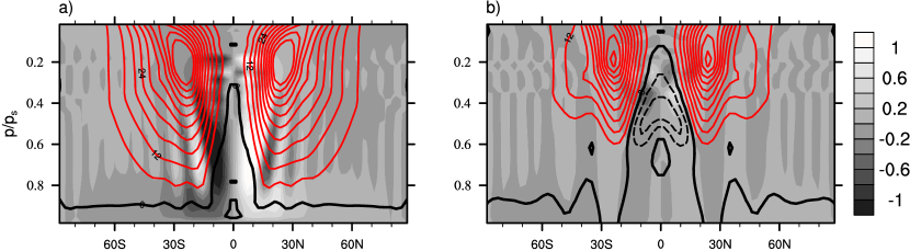
Figure 2: The axisymmetric zonal-mean zonal wind $\overline{u}$ [m s^-1] (contours) and mass streamfunction $\overline{\psi}\times 3\times 10^{-11}$ [kg s^-1] (in greyscale) for the control (HS-like) ($a$) and RTG ($b$) simulations at T170L30 resolution, with corresponding $\theta_{e}$ from Figure 1. Maximum and minimum values for $\overline{u}$ are $\pm$ 60 m s^-1, with contour interval 6 m s^-1. Negative $\overline{u}$ values are dashed (and in black) and positive are solid (and in red). The zero contour is drawn with double thickness. The light shading corresponds to the clockwise circulation and the dark shading corresponds to the anticlockwise circulation, respectively. No superrotation is present in the axisymmetric, eddy-free case.

$\begin{array}[]{cc}\includegraphics[width=433.62pt]{plots/Figure3a.pdf}\\ \includegraphics[width=433.62pt]{plots/Figure3b.pdf}\end{array}$

Figure 3: The time- and zonal-mean potential temperature $\overline{\theta}^{*}$[K], zonal wind $\overline{u}^{*}$ [m s^-1], and mass stream function $\overline{\psi}^{*}\times 3\times 10^{-11}$ [kg s^-1] for the fully turbulent three-dimensional control (HS-like) ($a$ and $c$) and RTG ($b$ and $d$) simulations at T170L30 resolution, with corresponding $\theta_{e}$ from Figure 1. The time averages are taken over $t=[700,1200]$ days ($a$ and $c$), and over $t=[4500,5000]$ days ($b$ and $d$). Contour values for $\overline{\theta}^{*}$ are the same as in Figure 1 and values for $\overline{u}^{*}$ and $\overline{\psi}^{*}$ are the same as in Figure 2. Clear superrotation is generated at the equator (at all altitudes) in the fully turbulent RTG simulation.

Note also that, apart from $F$, there are additional differences in the setup used in HS, Williams (2003) and the present study. For example, in Williams (2003) $\Delta\theta$ in equation (2.2) is not modulated by $\cos^{2}\!\phi$. In addition, $\tau=20$ days everywhere in this study – different than in HS, but the same as in Williams (2003). None of these differences qualitatively affect the results presented here, however.

The model domain, which extends vertically from $10^{3}$ hPa to $17$ hPa, is resolved by 30 levels equally spaced in $p$. Simulations are performed at {T42, T85, T170, T341} horizontal resolutions. The ‘control simulations’ (i.e. essentially HS simulations), with $\theta_{\text{e}}$ shown in Figure 1$a$, are integrated for $t=1200$ days; and, the ‘RTG simulations’, with $\theta_{\text{e}}$ shown in Figure 1$b$, are integrated for up to $t=7000$ days. In the latter simulations, equilibration takes longer at lower horizontal resolutions and/or with stronger dissipation. The timestep size $\Delta t$ (in seconds) is {600, 300, 150, 75} for the resolutions given above, respectively. The hyperdiffusion coefficient $\nu$ is chosen so that the $e$-folding time $\tau_{d}$ (in days) for the smallest scale in the system is {0.1, 0.01, 0.001, 0.0001}, respectively. Assuming

$$\tau_{d}\ \approx\ \frac{1}{\nu}\left[\frac{a^{2}}{N_{\mbox{\tiny T}}\,(N_{\mbox{\tiny T}}+1)}\right]^{4},$$ (5)

where $N_{\mbox{\tiny T}}$ is the spectral truncation wavenumber, the above $\tau_{d}$’s correspond to $\nu$ (in $10^{37}$ m⁸ s^-1) of {3.0, 0.1, 0.004, 0.0002}, respectively. Sensitivity of the results to horizontal resolution and hyperdissipation specifications is discussed in section 3.3.

3 Results

3.1 Mean circulation

Before describing the turbulent three-dimensional simulations, it is fruitful to examine the axisymmetric eddy-free circulation that results from prescribing the $\theta_{e}$ shown in Figure 1 and spinning up the atmosphere from an initially resting state. Figure 2 shows the resulting axisymmetric zonal-mean zonal wind and mass streamfunction ($\overline{u}$ and $\overline{\psi}$, respectively) from the control ($a$) and RTG ($b$) simulations at T170L30 resolution (i.e. T170 horizontal resolution with 30 vertical levels). The axisymmetric circulations are obtained by running the BOB model with no initial perturbation. Both simulations produce a weak Hadley circulation and the zonal flow consists of weak subrotation (easterly flow) at the equator and westerly jets centred at $\phi\approx\pm 25\degree$. However, the final axisymmetric circulation is dependent on the initial condition, in general.

Figure 3 shows the time- and zonal-mean potential temperature, zonal wind and mass streamfunction meridional cross-sections ($\overline{\theta}^{*}$, $\overline{u}^{*}$ and $\overline{\psi}^{*}$, respectively) from the fully turbulent, three-dimensional control ($a$​ and ​$c$) and RTG ($b$​ and ​$d$) simulations. Time-averaging is performed over $25\,\tau$’s after the simulations have reached a statistically equilibrated state, over the intervals $t~{}\!=\!~{}[700,1200]$ days for the control simulation and $t\!~{}\!=\!~{}[4500,5000]$ days for the RTG simulation.

$\begin{array}[]{ccc}\includegraphics[width=216.81pt]{plots/Figure4a.pdf}\includegraphics[width=216.81pt]{plots/Figure4b.pdf}\end{array}$

Figure 4: Eliassen-Palm flux vector, ${\bf F}=(F_{\phi},F_{p})$ [m² s^-2], and its divergence, $\nabla\!\cdot\!{\bf F}$ $\times 10^{9}$ [m s^-2], fields for the control ($a$) and RTG ($b$) simulations at T170L30 resolution averaged in time during the equilibrated stage. Negative $\nabla\!\cdot\!{\bf F}$ values are dashed (and in blue) and positive values are solid (and in red). $F_{\phi}$ and $F_{p}$ are scaled by 1 radian of latitude and 1 Pa of pressure, respectively.

In the control simulation, initially zonally-symmetric westerly jets (cf. Figure 2$a$) become baroclinically unstable and zonally-asymmetric flow develops. Following the onset of baroclinic instability, the jets move poleward and equilibrate at $\phi\approx\pm 45\degree$ (Figure 3$b$). The exact mechanism leading to the poleward migration is currently not well understood, but all of the proposed mechanisms involve some form of eddy-mean flow interaction (see e.g. Chen et al., 2007; Kidston and Vallis, 2010). Crucially, the flow remains weakly easterly at the equator, at all heights in the control simulation. Baroclinic eddies transport heat from low to high latitudes; as a result, the equator-to-pole temperature gradients are weaker in the equilibrated $\overline{\theta}^{*}$ distribution than in the prescribed $\theta_{\rm e}$ distribution (cf. Figure 3$a$ with Figure 1$a$). Note that the Hadley circulation in the fully non-linear simulation is mainly eddy-driven (cf. Figures 2$a$ and 3$c$).

In contrast, the equilibrated flow in the RTG simulation is superrotating at the equator when the eddies are present – and there at all altitudes, except at the very top (cf. Figures 2$b$ with Figure 3$d$). There is also a weak Hadley circulation in the RTG simulation in this case. Accordingly, the $\overline{\theta}^{*}$ distribution changes only slightly from the prescribed $\theta_{\rm e}$ distribution (cf. Figure 3$b$ with Figure 1$b$). This is consistent with the marked reduction in baroclinic instability observed in this simulation. The equilibrated subtropical jets remain close to their initial latitude (i.e. at $\phi\approx\pm 25\degree$) and take a much longer time to equilibrate, compared to the control simulation. The total (column-mean) equatorial zonal wind $\langle u_{\rm eq}\rangle$ undergoes rapid acceleration over $t=[200,1000]$ days, reaching statistical equilibration thereafter. Throughout this paper, this stage is referred to as the ‘equilibrated stage’ and the stage prior to this as the ‘acceleration stage’.

3.2 Wave-mean flow analysis

Acceleration of the zonal-mean zonal flow and direction of wave propagation can be assessed via the Eliassen-Palm (EP) flux vector, ${\bf F}=(F_{\phi},F_{p})$ (e.g. Andrews and McIntyre, 1978):

$$F_{\phi} = a\cos\phi\left[-\overline{u^{\prime}v^{\prime}}+\left(\frac{\overline{v^{\prime}\theta^{\prime}}}{\partial\overline{\theta}/\partial p}\right)\partial\overline{u}/\partial p\right]$$ (6)

$$F_{p} = a\cos\phi\left[(\overline{\zeta}+f)\left(\frac{\overline{v^{\prime}\theta^{\prime}}}{{\partial\overline{\theta}/\partial p}}\right)-\overline{u^{\prime}\omega^{\prime}}\right],\$$ (7)

where the primes denote deviations from the zonal mean, $v$ is the meridional velocity, $f=2\Omega\sin\phi$ is the Coriolis parameter, $\theta\equiv T(p/p_{s})^{\kappa}$ is the potential temperature and $\omega=Dp/Dt$ is the ‘vertical’ velocity. The second term in the brackets in equation (6) and the first (i.e. the $\overline{\zeta}$ term) and third terms in equation (7), which are the ageostrophic terms, are generally small compared to the remaining, geostrophic terms.

Figure 4 shows the EP flux vector field and its divergence, $\nabla\!\cdot\!{\bf F}$ (contours), for the control ($a$) and RTG ($b$) simulations. In the control simulation, the EP flux and its divergence follow the classic scenario: Rossby waves, generated near the surface by mid-latitude baroclinic instability, transport wave activity upward in the troposphere and equatorward at mid-height, transporting momentum poleward and heat upward and poleward. In the northern hemisphere, according to equation (6), $F_{\phi}<0$ implies $\overline{u^{\prime}v^{\prime}}>0$ (assuming the ageostrophic term to be small), leading to a poleward eddy momentum flux; correspondingly, according to equation (7), $F_{p}>0$ implies $f\overline{v^{\prime}\theta^{\prime}}>0$, leading to a poleward eddy heat flux. The vector field is divergent (positive) near the surface at mid- and high-latitudes and convergent (negative) in the upper troposphere and lower stratosphere, as well as in the equatorial region near the surface. According to the transformed Eulerian mean (TEM) equations (e.g. Andrews et al., 1987), zonal flow is accelerated (decelerated) in regions of positive (negative) $\nabla\!\cdot\!{\bf F}$; hence, the jet becomes increasingly barotropic.

In the RTG simulation, the transport of wave activity is upward and mainly poleward, unlike in the control simulation (see Figure 4$b$). The poleward heat flux is considerably weaker (n.b. the smaller reference vector magnitude in Figure 4$b$) and the flux activity is clearly dominant at higher altitudes (above $p\approx 600$ hPa level). The eddy momentum flux is mostly equatorward in both the northern and southern hemispheres. The $\nabla\!\cdot\!{\bf F}$ field is also weaker than in the control simulation (n.b. the smaller $\nabla\!\cdot\!{\bf F}$ values in Figure 4$b$) and displays a more complicated structure than in the control simulation. Significantly, a westerly zonal flow acceleration is present in the tropics, in the $p\approx[250,600]$ hPa region. Note also that at $p=200$ hPa, the zonal flow is accelerated at the equator and decelerated in the subtropics, in the $10\degree<|\phi|<30\degree$ region, where the wave propagation is equatorward. In addition, the poleward flanks of the subtropical jets are decelerated at higher altitudes ($p\approx[200,450]$ hPa) and accelerated at lower altitudes ($p\approx[450,600]$ hPa).

It is useful to examine the spectral characteristics of the eddy momentum flux convergence. For this, the eddy momentum flux at each $\phi$ is first spectrally decomposed among the zonal wavenumbers $\{m\}$ and the $m$–$\phi$ covariance spectrum is obtained before computing the divergence (e.g. Hayashi, 1971; Randel and Held, 1991). Similarly, the angular phase speed, $c_{A}\,(m,\phi)=\varpi a/m$ with $\varpi=\varpi(m)$ the frequency, is computed to obtain the $c_{A}$–$\phi$ spectrum. We use $c_{A}$ instead of phase speed $c$, because $c_{A}$ is conserved following a meridionally propagating Rossby wave packet in a zonally-symmetric background flow. Note that a positive (negative) region in the convergence spectrum is associated with a momentum source (sink). The convergence spectra from both the control and RTG simulations are shown in Figure 5. Spectra are taken from the $p=500$ hPa level, the level of maximum zonal wind acceleration in the RTG simulation (see Figure 4$b$). Recall that there is no superrotation in the control case.

First we discuss the $m$–$\phi$ spectra. Figure 5$a$ shows the $m$–$\phi$ spectrum calculated for ten consecutive 50-day windows over $t=[700,1200]$ days from the control simulation during the equilibrated stage. The spectrum for only $m\leq 10$ is shown because larger wavenumbers possess insignificant amplitudes. The spectrum shows that the modes of $m\!\approx\!6$, centered on the jets, dominate at mid-latitudes. Figure 5$b$ shows the corresponding $m$–$\phi$ spectrum from the RTG simulation in the equilibrated stage ($t=[4500,5000]$ days). The spectrum in this simulation is also dominated by $m\!\approx\!6$ modes, but the waves are excited on both flanks of the subtropical jets, at $\phi\approx\pm 5\degree$ and $\phi\approx\pm 35\degree$. These waves stir the flow and converge westerly momentum into their source region and easterly momentum into their breaking/saturation region. In addition, low wavenumber (i.e. $m\!\approx\!2$) modes converge westerly momentum at the equator. Later we show that the $m\!\approx\!2$ modes have a distinct Kelvin wave-like behaviour, as also identified by Potter et al. (2014) in their study.

$\begin{array}[]{cc}\includegraphics[width=216.81pt,height=398.33858pt]{plots/Figure5a.pdf}\hskip 19.91684pt\includegraphics[width=216.81pt,height=398.33858pt]{plots/Figure5b.pdf}\end{array}$

Figure 5: Eddy momentum flux convergence spectra $\times 10^{-6}$ [m s^-2] at $p=500$ hPa for the control and RTG simulations at T170L30 resolution: ($a$) and ($b$) show the $m$–$\phi$ spectrum and ($c$) and ($d$) show the $c_{A}$–$\phi$ spectrum (contours) as well as the angular velocity $\overline{u}/\cos\phi$ (red curve). The spectra are computed from ten 50-day windows over $t=[700,1200]$ days for the control simulation ($a$ and $c$) and over $t=[4500,5000]$ days ($b$ and $d$) for the RTG simulation. Negative contours are dashed and positive contours are solid. Notice the dominance of zonal wavenumbers $m\approx 6$ in both simulations. The phase speeds in the control simulation have values less than or comparable to $\overline{u}/\cos\phi$, whereas $c_{A}>\overline{u}/\cos\phi$ in the RTG simulation at the equator. Critical layers are located at latitudes where $c_{A}\approx\overline{u}/\cos\phi$. High phase speed, zonal wavenumber $m\!\approx\!2$ modes help to accelerate the zonal mean zonal flow at the equator in the RTG simulation.

There are other important, distinguishing features in the RTG simulations. For example, at lower model resolutions the convergence spectra exhibit significant qualitative differences, compared to the spectrum in Figure 5$b$. At resolutions lower than T170 (and assuming the nominal values for the hyper-dissipation coefficients (section 3.3)) the $m\!\approx\!6$ modes, which are located on the flanks of the subtropical jet, disappear completely after the initial acceleration stage. In the simulation presented in Figure 5$b$, these modes persist well into the equilibrated stage. As will be shown in section 3.3, the disappearance is due to inadequate horizontal resolution.

Now we discuss the $c_{A}$–$\phi$ spectra. Figures 5$c$​ and ​5$d$ present the $c_{A}$–$\phi$ spectra at the $p=500$ hPa level for the control ($c$) and RTG ($d$) simulations, respectively. Note that in both spectra, there is insignificant amplitude at $c_{A}\leq-10~{}$m s^-1 and $c_{A}\geq 45$ m s^-1. The spectra are obtained from the data over the same time windows as in the corresponding spectra in Figures 5$a$ and 5$b$. In Figures 5$c$ and 5$d$, the superimposed red curve shows angular velocity $\overline{u}_{A}=\overline{u}/\cos\phi$.

The mean flow acceleration is such that $\overline{u}_{A}$ evolves towards $c_{A}$ (e.g. Andrews et al., 1987; Holton and Lindzen, 1972). In Figure 5$c$, because $c_{A}\lesssim\overline{u}_{A}$ everywhere, the equatorward propagating Rossby waves can only decelerate the zonal flow. The waves, which are generated at the cores of the jets, propagate equatorward until they encounter a critical layer on the equatorward flanks of the jets. In the critical layer, Rossby waves break and deposit easterly momentum. Hence, no superrotation is present in the control simulation. In contrast, in Figure 5$d$ (RTG simulation), the $m\!\approx\!6$ modes that propagate poleward from their source region at $\phi\approx\pm 5\degree$ deposit westerly momentum near the equator where $c_{A}\gtrsim\overline{u}_{A}$. These waves break at $\phi\approx\pm 15$–$20\degree$ and decelerate the flow there. While the $m\!\approx\!6$ modes are only able to accelerate the flow at $\phi\approx\pm 5\degree$, the $m\!\approx\!2$ modes (with $c_{A}\approx 30$ m s^-1) accelerate the zonal flow at the equator by converging westerly momentum and forcing $\overline{u}_{A}$ towards $c_{A}$ throughout the duration of the simulation.

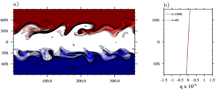
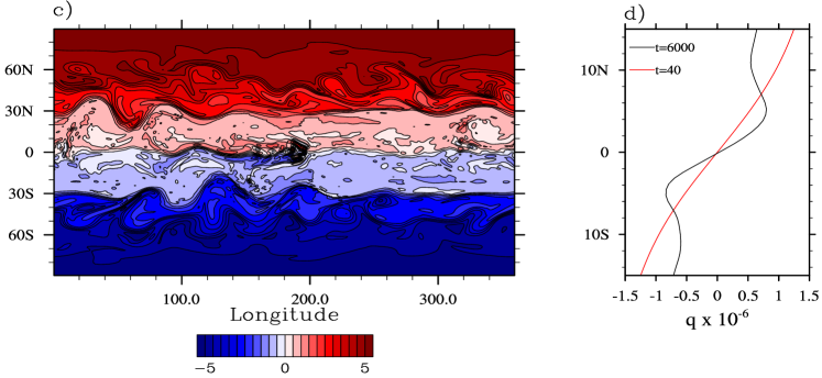
Figure 6: Snapshot of Ertel potential vorticity $q\times 10^{-6}$ [K m² kg^-1 s^-1] and its zonal-mean $\overline{q}$ for the control simulation ($a$ and $b$) and RTG simulation ($c$ and $d$) at T170L30 resolution. The $q$ fields are shown at $t=1000$ days in ($a$) and at $t=6000$ days in ($c$) in cylindrical-equidistant projection on the $\Theta=315$ K and $\Theta=300$ K isentropes, respectively. The $m\!\approx\!6$ mode can be seen in ($a$) and ($c$), as well as the presence of equatorial $q$-gradients and blobs in ($c$) (only). $\overline{q}$ in the equatorial region is shown in ($b$) and ($d$) on the same isentropes and at the same times as in ($a$) and ($c$). $\overline{q}$ at $t=40$ days (red) is also shown. Superrotation is generated in the RTG simulation as a consequence of extrusion of high $q$ from higher latitudes to the equator in the northern hemisphere via stirring. In contrast, notice the absence of $q$-stirring at the equator in the control simulation.

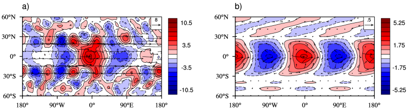
Figure 7: Composites of perturbation geopotential height $\Phi^{\prime}$ [m² s^-2] with perturbation horizontal wind vectors overlaid for the RTG simulation at T170L30 resolution. The fields are shown in cylindrical-equidistant projection for $|\phi|<\pm 60\degree$ at the $p=500$ hPa level. The unfiltered fields are shown in ($a$). The fields filtered so that only $m=2$ signal remains are shown in ($b$). Note the resemblance of the filtered fields with the classic Kelvin wave solution.

$\begin{array}[]{cccc}\includegraphics[width=216.81pt]{plots/Figure9a.pdf}\hskip 14.22636pt\includegraphics[height=156.49014pt,width=216.81pt]{plots/Figure9b.pdf}\\ \includegraphics[width=216.81pt]{plots/Figure9c.pdf}\hskip 14.22636pt\includegraphics[height=156.49014pt,width=216.81pt]{plots/Figure9d.pdf}\\ \end{array}$

Figure 8: Symmetric and antisymmetric mode Wheeler-Kiladis diagrams of the geopotential height field in the equatorial region ($|\phi|<10\degree$) for the control ($a$ and $c$) and RTG ($b$ and $d$) simulations at $p=500$ hPa. The linear dispersion curves for Kelvin and mixed Rossby-gravity waves for equivalent depths $h_{0}=12,40,$ and $100$ m are overlaid on the diagrams. Notice the $h_{0}=100$ m Kelvin wave in the RTG simulation.

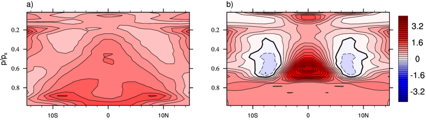
Figure 9: Time- and zonal-mean meridional gradient of quasi-geostrophic potential vorticity $\partial\overline{Q}/\partial\phi$ [normalized by $2\Omega$], pressure vs. latitude, for the control ($a$) and RTG ($b$) simulations at T170L30 resolution in the equatorial region. Negative $\partial\overline{Q}/\partial\phi$ values are dashed (and in blue) and positive are solid (and in red). The zero contour is drawn with double thickness. Note the reversal of $\partial\overline{Q}/\partial\phi$ sign in the equatorial region of the RTG simulation.

$\begin{array}[]{cccc}\includegraphics[width=286.19078pt]{plots/Figure10a.pdf}\includegraphics[width=143.09538pt]{plots/Figure10b.pdf}\end{array}$

Figure 10: Hovmöller diagrams of the perturbation geopotential height field $\Phi^{\prime}$ [m² s^-2] at $p=500$ hPa in the beginning of the RTG simulation. The $\Phi^{\prime}$ field filtered for $m=6$ is shown at $\phi=10\degree$ N in $a$). The $\Phi^{\prime}$ field filtered for $m=2$ is shown at $\phi=10\degree$ N in $b$) and at the equator in $c$). The $m=6$ subtropical Rossby waves are generated before the equatorial $m=2$ Kelvin waves.

For a more detailed view of the flow field at equilibrated stage, a snapshot of Ertel potential vorticity, $q=[(\zeta+f)\!\cdot\!\nabla\theta]\,/\,\rho$, is shown in Figure 6; here $\rho$ is the density and the projection shown is cylindrical-equidistant centered on the equator. Figure 6$a$ shows $q$ for the control simulation at $t=1000$ days, on the $\theta=315$ K isentrope. Figure 6$c$ shows $q$ for the RTG simulation at $t=6000$ days, on the $\theta=300$ K isentrope. Both isentropes lie approximately on the $p=500$ hPa surface in the tropics. Both simulations are at T170L30 resolution. To illustrate how the PV distribution changes from the initial stage, the zonal-mean PV ($\overline{q}$) for snapshots in Figures 6$a$ and 6$c$ is shown in the equatorial region in Figures 6$b$ and 6$d$ (black curves) together with $\overline{q}$ at $t=40$ days (red curve). Note that at $t=40$ days the unaveraged flow in both simulations is nearly axisymmetric, but becomes increasingly non-axisymmetric over time.

The $m\!\approx\!6$ structure can clearly be seen in Figures 6$a$ and 6$c$, but stirring of $q$ occurs closer to the equator in the RTG simulation than in the control simulation (6$c$ and 6$a$, respectively). This is consistent with the diagnostics in Figure 5 discussed above. In the control simulation no stirring is taking place in the equatorial region as the zonal-mean PV changes little from the zonally-symmetric PV at $t=40$ days (see Figure 6$b$). Crucially, in the RTG simulation, stirring results in a band of steep $q$-gradient, which is pushed to the equator; a corresponding band is not present in the control simulation. The band is not zonally-symmetric and often appears with a blob of $q$ that appears to have broken off from large-amplitude undulations of the high-gradient band to the north (south) of the equator in the northern (southern) hemisphere. In addition to inducing a ‘$q$-jump’ at the equator, the undulations and concentrations of large-amplitude PV at the equator, act as sources of enhanced superrotation. The blobs of $q$ at the equator translate longitudinally faster than the zonal mean zonal wind and manifest themselves in the convergence spectrum as the $m\approx 2$ Kelvin wave-like features (see Figure 5$b$). Note that in the presence of meridional shear in the background flow, Kelvin waves perturb meridional velocity and hence $q$ (e.g. Iga and Matsuda, 2004).

While the $m\approx 2$ features lack a coherent wave-like structure in the $q$ field in Figure 6$c$, the wave-like behaviour is more clearly visible in the perturbation geopotential height field $\Phi^{\prime}$ in the equatorial region of the RTG simulation. Figure 7 shows composites of $\Phi^{\prime}$ and perturbation horizontal wind vectors on the $p=500$ hPa surface for the RTG simulation. The composites are constructed from the $m-\varpi$ spectrum from the equilibrated fields. The spectrum is filtered by removing all westward propagating signal, eastward propagating signals with frequencies below 1/30 day^-1 and above 1/4 day^-1, and $m$ below 1 and above 6. An inverse transform is then applied to reconstruct the filtered time series and the entire fields are regressed against the filtered time series at a base point on the equator, where the wave variance is maximum. In ($a$) the complete composited fields are shown and in ($b$) the fields have been filtered to accentuate the $m=2$ signal.

The filtered fields in particular, resemble the classic Kelvin wave solution for the equatorial beta-plane shallow water model (e.g., Matsuno, 1966). By examining the time-lagged composites, we have found that the $m=2$ signal in Figure 7$b$ is only coherent up to $\phi\approx\pm 15\degree$ (not shown). Linear resonance between equatorial Kelvin waves and subtropical Rossby waves via ageostrophic instability is proposed by Wang and Mitchell (2014) to drive superrotation under zonally-symmetric thermal forcing. Such instability would have a distinct Kelvin-wave like structure at the equator (see e.g. Figure 1 in Wang and Mitchell (2014)). However, the linear Rossby-Kelvin instability also requires matching phase speeds between the two types of waves, since the wavenumber $m$ is fixed in the linear resonance analysis. In Figure 5$d$, however, the phase speed of the subtropical Rossby waves ($c_{A}\approx 10$ m s^-1) is clearly different than the phase speed of the equatorial Kelvin waves ($c_{A}\approx 30$ m s^-1). This is so even during the acceleration stage of the well-resolved RTG simulation (not shown). Hence, the linear Rossby-Kelvin wave instability is not the likely mechanism generating and maintaining superrotation in the RTG simulations. Instead, as in (Williams, 2003), it appears that here the barotropic instability on the equatorward flank of the westerly subtropical jets stirs the flow and excites equatorial Kelvin waves.

Kelvin waves in the RTG simulation can be further identified by Fourier transforming equatorial geopotential height field $\Phi$ in space and time and depicting the resulting spectra in the Wheeler-Kiladis diagrams as a function of $\varpi$ and $m$ (Wheeler and Kiladis, 1999). Here ten 96-day time windows are taken to obtain the $\Phi$ spectrum. In Figure 8, both symmetric ($a$ and $b$) and antisymmetric ($c$ and $d$) Wheeler-Kiladis diagrams for the control ($a$ and $c$) and RTG simulations ($b$ and $d$) at T170L30 resolution are shown at the $p=500$ hPa level. Overlaid on the symmetric diagrams are the linear dispersion curves for the Kelvin waves and on the antisymmetric diagrams the linear dispersion curves for the mixed Rossby-gravity waves for equivalent depths of $h_{0}=12,40,$ and $100$ m, respectively.

For the control simulation, only a weak Kelvin wave signal is present at the equator (Figure 8$a$) and the spectrum is dominated by the westward propagating mixed Rossby-gravity waves with $h_{0}=100$ m (Figure 8$c$). For the RTG simulation, a clear $h_{0}=100$ m Kelvin wave signal dominates the spectrum (Figure 8$b$) with little or no westward propagating wave activity. The phase speed of the $h_{0}=100$ m Kelvin waves is $\approx\!30$ m s^-1, suggesting that Kelvin waves are important in driving and maintaining superrotation in the RTG simulations (cf. Figure 5$d$). We note that the equatorial $\Phi$ spectra is of lower amplitude in simulations with lower horizontal resolution after the acceleration stage.

To establish the role of shear instabilities in Kelvin wave excitation, it is instructive to examine the meridional gradient of the zonal-mean PV in the equatorial region. As in Williams (2003), we show quasi-geostrophic time- and zonal-mean PV $\partial\overline{Q}/\partial\phi$ (scaled by 2$\Omega/a$) in Figure 9 for the control ($a$) and RTG ($b$) simulations, respectively. In Figure 9$b$ $\partial\overline{Q}/\partial\phi$ changes sign on the equatorward flank of the subtropical jet, at $\phi=\pm 5\degree$ in the $p=[200,700]$ hPa vertical region throughout the RTG simulation. The reversal of the gradient at $\phi=\pm 5\degree$ is due to the barotropic component (i.e. the meridional gradient of the absolute vorticity) of $\partial\overline{Q}/\partial\phi$ (not shown). Hence, the source of the $m\!\approx\!6$ Rossby waves on the equatorward flanks of the jets and the equatorial $m\!\approx\!2$ Kelvin waves is likely the barotropic, Rayleigh-Kuo, instability. The (latitudinal) deformation length scale $L_{\text{D}}$ of an equatorially trapped Kelvin wave is roughly $L_{\text{D}}=\sqrt{c/\beta}$, where $\beta=2\Omega/a$. For the wave with $c\approx 30$ m s^-1 (cf. Figures 5$d$ and 8$b$), $L_{\text{D}}\approx 1200$ km or $\phi\approx\pm 10\degree$. Therefore, to excite equatorially trapped Kelvin waves, stirring must occur within the $\phi\approx\pm 10\degree$ band centered on the equator. This occurs in the RTG simulation. For the control simulation, the necessary condition for neither the barotropic (see Figure 9$a$) nor the baroclinic instability is satisfied in this region in the time- and zonal-mean, which likely explains the weak equatorial Kelvin wave signal in the control simulation (see Figure 8$a$).

That stirring in the subtropics (within $L_{\text{D}}$) by the $m\approx 6$ Rossby waves precedes the generation of equatorial $m\approx 2$ Kelvin waves (with $c\approx 30$ m s^-1) in the RTG simulation can be seen in Hovmöller diagrams in Figure 10. The figure shows $\Phi^{\prime}$ at $p=500$ hPa in the beginning of the simulation. The $\Phi^{\prime}$ field filtered for $m=6$ is shown at $\phi=10\degree$N in ($a$). The $\Phi^{\prime}$ field filtered for $m=2$ is shown at $\phi=10\degree$N in ($b$) and at the equator in ($c$). The Kelvin waves are excited at $t\approx 110$ days (Figures 10$b$ and $c$), after the development of the $m=6$ Rossby waves at $t\approx 80$ days (Figure 10$a$). These waves continue to propagate eastward throughout the simulation (not shown).

In summary, the following mechanisms contribute to generating and/or maintaining superrotation in well-resolved RTG simulations:

• Mechanical stirring inside the latitudinal range of the deformation length scale $L_{\text{ D}}$ from the equator, is required to excite $m\approx 2$ Kelvin waves under statically stable zonally-symmetric thermal forcing. Here the source of the stirring is barotropic instability (with predominantly $m\approx 6$ signal) on the equatorward flank of the subtropical westerly jet.

• Since Kelvin waves are not excited if the stirring occurs at latitudes outside $L_{\text{ D}}$, the specified equilibrium temperature profile has to produce and maintain westerly jets that are unstable to shear instabilities within $L_{\text{ D}}$ from the equator.

3.3 Resolution and dissipation

We have seen that superrotation may be generated and maintained by wave-mean flow interaction. However, in the RTG simulations, a stronger superrotation is also clearly produced at lower horizontal resolution. This indicates that part of the superrotation is of numerical origin. In general, the strength of superrotation depends sensitively on the horizontal resolution and dissipation. We have found that relatively high horizontal resolution ( $\gtrsim\!$ T170) is required for numerical convergence – particularly for the RTG case. Among other things, the high resolution ensures accurate representation of the eddy fluxes.

In this study, simulations are defined to be converged if both of the following criteria on the total (column-averaged) equatorial zonal wind $\langle u_{\rm eq}\rangle$—averaged over the $\phi=\pm 5\degree$ band centered on the equator—are met:

i) At equilibration, $\langle u_{\rm eq}\rangle$ is statistically the same at least at two different horizontal resolutions, with a given viscosity coefficient $\nu$.

ii) At equilibration, $\langle u_{\rm eq}\rangle$ is not sensitive to the choice of viscosity coefficient $\nu$, at a given horizontal resolution.

Criterion i) tests for ‘numerical’ convergence while criterion ii) tests for ‘physical’ convergence. At very high Reynolds number, a simulation (particularly the large scales in it) should not be sensitive to the choice of numerical viscosity coefficient $\nu$, whose primary purpose is to remove enstrophy near the grid-scale and to prevent the simulation from blowing up. For criterion ii), $\nu$ values are heuristically chosen from a ‘credible’ range, by which reference is made to those values that permit the vorticity field to be neither under-dissipated (i.e. inundated with grid-scale noise) nor over-dissipated (i.e. devoid of any strong coherent structures, such as vortices and sharp gradients). Experience has shown that a certain amount of tuning is always necessary and that there always exists a finite range of values that is reasonably free from gross subjectivity and satisfies the credibility condition on the vorticity field. Each new problem and setup necessitates a thorough characterization of accuracy and convergence for confidence in the obtained results.

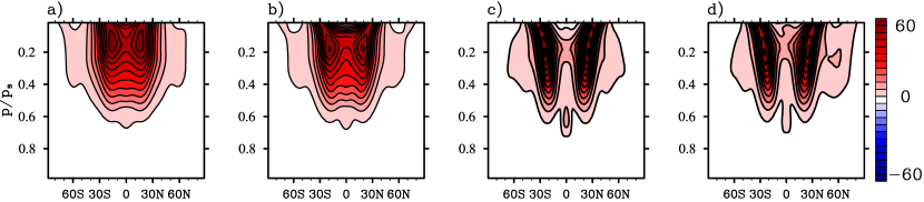
Figure 11: The time- and zonal-mean zonal wind $\overline{u}^{*}$ [m s^-1] for the RTG simulation at T42L30 ($a$), T85L30 ($b$), T170L30 ($c$) and T341L30 ($d$) resolutions. Contour intervals are the same as in Figure 2. Subtropical jets diffuse together at the equator much more strongly at low resolution.

Before we discuss $\langle u_{\rm eq}\rangle$, the equilibrated $\overline{u}^{*}$ from the RTG simulations at T42L30 ($a$), T85L30 ($b$), T170L30 ($c$) and T341L30 ($d$) resolutions is presented in Figure 11. The figure clearly shows that RTG simulations are not converged at resolutions lower than T170L30, as they do not satisfy criterion i). The T170 and T341 results are very similar. In contrast, the equilibrated $\overline{u}^{*}$ for the control simulations can exhibit qualitatively the same behaviour at the same four horizontal resolutions presented (although they are still not converged, as is also discussed below). Interestingly, as can be seen in the figure, superrotation is considerably stronger at lower horizontal resolution in the RTG simulations, as already mentioned.

Figure 12 now shows the time series of $\langle u_{\rm eq}\rangle$ from the control (Figure 12$a$) and RTG (Figure 12$b$) simulations. For reference, the time series from the T341L30 RTG simulation is also shown in Figure 12$b$. Note that, with exceptions as noted in the discussion below, the value of $\nu$ for all the simulations in the figure is chosen so that the $e$-folding time for the truncation scale is nominally $\{0.1,\,0.01,\,0.001,\,0.0001\}$ days at {T42, T85, T170, T341} resolutions, respectively. The chosen times correspond to $\nu=$ {3.0, 0.1, 0.0044, 0.00017}$\times 10^{37}\!$ m⁸ s^-1, respectively. All simulations are with L30 vertical resolution.

Figure 12$a$ shows that the convergence criterion i) is fulfilled for the control simulation at T42 resolution. However, the control simulation does not fulfill criterion ii) at resolutions lower than T85. For example, a T42 resolution simulation employing the $\nu$ value from the T21 resolution simulation (i.e. 25 times greater value) leads to a significantly different time series behaviour (cf. black and green lines); the behaviour does not persist into T85 resolution simulations, as is shown below. Convergence criterion i) is also fulfilled by the RTG simulation – but at much higher (T170) resolution. Moreover, the value of $\langle u_{\rm eq}\rangle$ at equilibration for the converged RTG simulations is much lower than for the un-converged, lower-resolution simulations, by as much as 17 m s^-1 (cf. black and blue curves in Figure 12$b$); this is consistent with the behaviour in Figure 11. In addition, RTG simulations at T42 and T85 resolutions take a considerably longer time to reach equilibration than that at T170 resolution; in the latter case, equilibration is reached at $t\!\approx\!1000$ days, compared with $t\!\approx\!7000$ days for the former cases.

$\begin{array}[]{cc}\includegraphics[height=142.26378pt,width=216.81pt]{plots/Figure12a.pdf}\includegraphics[height=142.26378pt,width=216.81pt]{plots/Figure12b.pdf}\end{array}$

Figure 12: Time series of column-averaged zonal wind at the equator $\langle u_{\rm eq}\rangle$ [m s^-1] at varying horizontal resolutions for the control ($a$) and RTG ($b$) simulations: $\langle u_{\rm eq}\rangle$ for {T42L30, T85L30, T170L30, T341L30} resolutions are shown in {black, red, blue, yellow}, respectively. The green curve in $a$) shows the control simulation performed at T42 horizontal resolution with $\nu$ from a T21 resolution simulation, which is 25 times larger than in the ‘nominal’ T42 simulation (black curve). The green curve in $b$) shows the RTG simulation performed at T170 horizontal resolution with $\nu$ the same as in the T85 resolution simulation (red curve). The magnitude of $\langle u_{\rm eq}\rangle$ is insensitive to the horizontal resolution in the control simulations – when properly tuned, whereas $\langle u_{\rm eq}\rangle$ decreases with increasing resolution in the RTG simulations. In the latter simulations, T170L30 simulations with different $\nu$ produce nearly-identical results.

$\begin{array}[]{cc}\includegraphics[height=142.26378pt,width=216.81pt]{plots/Figure13a.pdf}\includegraphics[height=142.26378pt,width=216.81pt]{plots/Figure13b.pdf}\end{array}$

Figure 13: Time series of $\langle u_{\rm eq}\rangle$ [m s^-1] at T85L30 resolution with varying $\nu$ for the control ($a$) and RTG ($b$) simulations. The viscosity coefficient $\nu$ is chosen so that $\tau_{\rm d}$ is 0.001 days (black curve), 0.01 days (red curve) and, 0.1 days (purple curve). In addition, $\langle u_{\rm eq}\rangle$ from the nominal T170L30 simulation is plotted in $b$). Note the insensitivity of the control simulations to $\nu$ but the reduction of $\langle u_{\rm eq}\rangle$ with decreasing $\nu$ in the RTG simulations. Note also that T170L30 results are the same as T85L30 results with $\tau_{\rm d}=0.1$ days in $b$).

Throughout this work, a larger value of $\nu$ is used when performing a given simulation at a lower horizontal resolution – as is commonly practiced in numerical simulations. Alternatively, a smaller value of $\nu$ is used when performing a given simulation at a higher horizontal resolution. The practice is primarily carried out for numerical stability and/or ‘spectrum tuning’ reasons, and it results in different damping times for a given wavenumber at the different resolutions. However, as advocated in Polvani et al. (2004) and Polichtchouk and Cho (2012), the same value of $\nu$ should be used for all resolutions in order to ‘cleanly’ assess numerical convergence: each wavenumber, up to the truncation, then experiences the same dissipation rate for a given simulation. This philosophy is closely related to convergence criteria i) and ii). All imply that once simulation is adequately resolved, including additional, higher wavenumbers in the simulation would not significantly affect the large-scale flow. Criterion ii), in particular, ensures that most ‘stable’ value of $\nu$ is used when assessing convergence, since there exists a finite range of values which prevent a simulation from blowing up. Of course, all this assumes weak (or absence of) spectral non-locality of the flow, which generally appears not to be the case in practice.

Consider the green and red curves in Figure 12$b$, showing two RTG simulations at different horizontal resolutions (T85 and T170) using the same $\nu$ value. It is clear that the RTG simulation is not converged at T85 resolution since the two curves deviate from each other; on the other hand, the curves for T170 and T341 resolutions, subjected to the same test, do match very closely. In fact, in general, the disagreement is much stronger, than in the control case (cf. green and black curves in Figure 12$a$). Clearly, the ‘extra modes’ included in the T170 resolution affect $\langle u_{\rm eq}\rangle$ quantitatively in the RTG simulations.

Figure 13 illustrates the above points more explicitly with simulations at T85L30 resolution, for the control (Figure 13$a$) and RTG (Figure 13$b$) cases. Criterion i) is met for the control case at T85 resolution, and has already been discussed above. Figure 13$a$ demonstrates that criterion ii) is also met: the simulations are not sensitive to variations in $\nu$, suggesting the control case is converged at T85 resolution. In contrast, Figure 13$b$ demonstrates that criterion ii) is not met for the RTG case: the simulations are acutely sensitive to variations in $\nu$. Moreover, superimposing the time series from the T170 resolution simulation illustrates that it is possible to erroneously conclude that criterion i) is met (see the blue and purple curves), if $\nu$ were not varied at the T85 resolution; and significantly, the equatorial superrotation is surprisingly weaker at the higher resolution. It is important to reiterate at this point that the ‘correct’ $\nu$ at T85 resolution cannot be determined a priori: it is only after performing the RTG simulation at T170L30 resolution and establishing that the converged simulations have $\langle u_{\rm eq}\rangle\approx 5$ m s^-1 that it is possible to tune $\nu$ for an ‘optimal’ simulation.

Superrotation is stronger in the lower-resolution and/or stronger-dissipation simulation, due to diffusion of $q$. In those simulations, $q$-contours are more diffused in the subtropics. Hence, the resulting jets are less sharp on their equatorward flanks and the flow is more strongly superrotating at the equator (cf. Figures 11$a$–$d$). The mechanism can be clearly seen in Figure 14, which shows the $q$ distributions on the $\theta=330$ K isentrope from two RTG simulations (T42 and T170 resolutions) at $t=5000$ days. The $q$-gradients are clearly sharper at $\phi\approx\pm 25\degree$ and the equatorial $q$-step is wider in the T170 resolution simulation – i.e., the jets across the equator are much less ‘fused’ into each other. It is important to understand that this is an entirely different mechanism than the ‘barotropic instability exciting equatorial Kelvin waves’ mechanism discussed in section 3.2.

In addition, in under-resolved and/or over-dissipated simulations the meridional shear on the equatorward flanks of the subtropical jets is reduced as the jets are ‘fused’ into each other. Therefore it becomes increasingly harder to satisfy the Rayleigh-Kuo instability criterion in the time- and zonal-mean, following the acceleration stage (e.g., at T42 resolution this occurs at $t=400$ days). This results in the mitigation of nonlinear mixing of $q$ at the equatorward flanks of the subtropical jets. The $m\!\approx\!6$ eddies at $\phi\approx\pm 10\degree$–$25\degree$ (Figure 5; see also Figure 6) are completely absent in the equilibrated stage in the low-resolution/high-dissipation simulations. Note that the Kelvin waves can still be excited in under-resolved and over-dissipated simulations as the $\partial\overline{Q}/\partial\phi$ continues to change sign at $\phi\approx\pm 5\degree$. The reversal of the $\partial\overline{Q}/\partial\phi$ sign in this case is, however, due to the baroclinic component. The Kelvin wave amplitude in the equilibrated stage is, however, by as much as $\approx 30\%$ weaker than in the converged simulations.

To summarize:

• Compared to the control simulation, high ( $\gtrsim\!$ T170) horizontal resolution is required for numerical convergence in the RTG simulation.

• In low-resolution/high-dissipation RTG simulations superrotation is artificially enhanced as the linear diffusion of $q$ ‘fuses’ the subtropical jets together on their equatorward flanks. This creates an artificial source of superrotation as the flanks of the westerly jets overlap at the equator.

• Because the $q$-gradients on the equatorward flanks of the subtropical jets are less sharp, barotropic instability is weaker or absent in the under-resolved/over-dissipated RTG simulations. This mitigates non-linear mixing of $q$ by the barotropic $m\approx 6$ eddies at $\phi\approx\pm 10\degree$–$25\degree$.

• ‘Numerical diffusion’ mechanism is entirely different from the ‘barotropic instability exciting Kelvin waves’ mechanism for generating and maintaining superrotation, discussed in the preceding subsection.

$\begin{array}[]{cc}\includegraphics[height=270.30118pt,width=281.85034pt]{plots/Figure14a.pdf}\includegraphics[height=270.30118pt,width=108.405pt]{plots/Figure14b.pdf}\end{array}$

Figure 14: Potential vorticity field, $q\times 10^{-6}$  [K m² kg^-1 s^-1], in cylindrical-equidistant projection on the $\Theta=330$ K isentrope (approximately at $p=200$ hPa in the tropics) and $t=5000$ days for the RTG simulation at T42L30 ($a$) and T170L30 ($c$) resolutions. Notice the weaker $q$-gradients in the subtropics and narrower equatorial $q$-step at T42 horizontal resolution. In $b$) and $d$), $\overline{q}$ (black curve) and zonal-mean $\overline{u}$ (red curve) for the simulations shown in $a$) and $c$), respectively. At low resolution, the subtropical jets are more diffused and broader than at high resolution. At high resolution mixing of $q$ on the equator-ward flanks of the jets is stronger. As a consequence, superrotation is actually stronger at low resolution.

3.4 Other sensitivities

In addition to resolution and dissipation, the strength of superrotation in the RTG simulations is sensitive to parameters in the equilibrium temperature distribution, such as {$\gamma$, $b$, $\Delta T$, $T_{\rm s}$} in equation (2.2). Recall that the following criteria on the westerly jets must be met for generation of superrotation in fully resolved simulations: 1) weak mid-latitude baroclinic instability; and 2) shear instability within the deformation length scale of an equatorial Kelvin wave. If the specified equilibrium temperature distribution produces westerly jets that do not meet the above criteria, superrotation does not occur. For example, for $\gamma\geq 0.05$ or $b<4$, transition to superrotation does not occur — especially in high-resolution/low-dissipation simulations. For a larger $\gamma$ baroclinic instability becomes stronger as the near-surface equator-to-pole temperature gradient is increased. However, a transition is still possible if $b>4$ for the same $\gamma$ ($\geq 0.05$) because baroclinic instability is then confined to lower latitudes (Williams, 2003). For smaller $b$ the subtropical jets are located too far from the equator for criterion 2) to be satisfied. Setting $\Delta T>60$ K (and keeping all other parameters the same) also produces stronger superrotation because stronger meridional shear on the equatorward flanks of the subtropical jets more strongly satisfies the necessary criterion for barotropic instability than in the nominal RTG case.

The magnitude of superrotation in the RTG simulation is also somewhat sensitive to the form of the initial perturbation. A north-south symmetric perturbation—such as a small amplitude localized bump at $(\pm\!\phi_{0},\lambda_{0})$ or a pure spherical harmonic mode perturbation—produces north-south symmetric circulation and considerably stronger superrotation than in the simulations initialized with north-south asymmetric perturbation—such as Gaussian white noise. In such north-south symmetric simulations, the equatorial flow is purely zonal (i.e., does not meander) and as a result the superrotation is stronger.

It is also worth noting that superrotation is generated in the RTG simulation started from rest even in the absence of the Rayleigh drag. Hence, superrotation can occur on planets with no solid surface as long as the equator-to-pole equilibrium temperature gradient is weakened in the region below where the superrotating flow occurs. In summary, it appears that superrotation can be generated and maintained under a surprisingly wide range of conditions, in general.

4 Conclusions

In this paper, we have shown that equatorial superrotation can be readily generated, if the equator-to-pole surface temperature gradient is weak. This is so even under zonally-symmetric, statically-stable, thermal forcing in many cases. However, in general, superrotation does not arise as easily under zonally-symmetric forcing. Superrotation can be maintained under this situation if stirring from a near-equatorial barotropic instability is continuously provided.

When the equator-to-pole surface temperature gradient is reduced, the role of Rossby waves produced by mid-latitude baroclinic instability in converging easterly momentum into the equatorial region is diminished. Also, if a wave ‘source’ exists at the equator (e.g. in the form of stirring), superrotation can develop if the eddy angular momentum fluxes out of the region are strong enough and directed up the mean angular momentum gradient. Similar to Williams (2003) and Mitchell and Vallis (2010), we also observe in this study that barotropic instability generates equatorial superrotation in the zonally-symmetric RTG setup: the instability excites equatorial Kelvin waves, which are important for flow acceleration at the equator. In the control simulation the necessary criterion for barotropic or baroclinic instability is satisfied too far from the equator – outside the deformation length scale distance of a Kelvin wave – for the instabilities to influence equatorial dynamics. Barotropic instability might also be the source of Kelvin wave-like disturbances that produce superrotation in small $a$ or $\Omega$ regimes in Potter et al. (2014). For a fixed phase speed, the meridional width of a Kelvin wave increases with decreasing $a$ (and $\Omega$). Thus, the Rayleigh-Kuo instability criterion does not need to be satisfied as close to the equator as in the RTG simulations with Earth’s $\Omega$ and $a$, discussed in this paper. In contrast to what is suggested in Potter et al. (2014), according to this study, it is likely that the Kelvin wave mechanism they propose must be accompanied by a simultaneous occurrence of barotropic (or other shear) instability, in simulations with statically-stable, zonally-symmetric forcing.

The barotropic instability is not, however, the only mechanism responsible for superrotation in the RTG setup. Numerical diffusion (both implicit and explicit) generates artificially strong superrotation in under-resolved and/or over-dissipated RTG simulations. In this study, it is found that to adequately resolve the dynamics of angular momentum fluxes near the equator, relatively high horizontal resolution is required ( $\gtrsim\!$ T170). In low resolution or strongly dissipated simulations, potential vorticity is more spread out by diffusion than in the high resolution or low dissipation simulations. Consequently, in the under-resolved cases the subtropical jets are less sharp on their equatorward flanks. The flanks overlap at the equator and this provides an additional source of superrotation. In addition, weaker potential vorticity gradients mitigate barotropic instability and mixing by the $m\!\approx\!6$ Rossby waves, equatorward of $\phi\approx\pm 25\degree$. This allows the subtropical jets to further ‘fuse’ into each other.

Given the foregoing, the relative contributions of barotropic instability and numerical diffusion to superrotation generation can be adequately quantified only after thoroughly assessing numerical convergence of the simulations. The stronger resolution requirement for the RTG simulation, compared to the control simulation (which is converged at T85 horizontal resolution), is due to the near-equatorial location of the mixing region in the RTG simulations. When the subtropical jets (and hence the mixing zone) are located further poleward, low resolution or high dissipation can still induce superrotation.

References

- Andrews et al. (1987) Andrews DG, Holton JR, Leovy CB. 1987. Middle atmosphere dynamics. No. 40. Academic press
- Andrews and McIntyre (1978) Andrews DG, McIntyre ME. 1978. Generalized Eliassen-Palm and Charney-Drazin theorems for waves on axisymmetric mean flows in compressible atmospheres, J. Atmos. Sci., 35, 175–185.
- Arnold et al. (2012) Arnold NP, Tziperman E, Farrell B. 2012. Abrupt transition to strong superrotation driven by equatorial wave resonance in an idealized GCM. J. Atmos. Sci., 69, 626–640. DOI:10.1175/JAS-D-11-0136.1
- Asselin (1972) Asselin R. 1972. Frequency filter for time integrations, Mon. Wea. Rev., 100, 487–490. DOI: 10.1175/1520-0493(1972)100<0487:FFFTI>2.3.CO;2
- Chen et al. (2007) Chen G, Held IM, Robinson WA. 2007. Sensitivity of the latitude of the surface westerlies to surface friction. J. Atmos. Sci., 64, 2899–2915. DOI: 10.1175/JAS3995.1
- Dritschel and McIntyre (2008) Dritschel DG, McIntyre ME. 2008. Multiple jets as PV staircases: The Phillips effect and the resilience of eddy-transport barriers. J. Atmos. Sci., 65, 855–874. DOI: 10.1175/2007JAS2227.1
- Hayashi (1971) Hayashi Y. 1971. A generalized method of resolving disturbances into progressive and retrogressive waves by space Fourier and time cross-spectral analysis, J. Meteorol. Soc. Jpn., 49, 125–128.
- Held and Hoskins (1985) Held IM, Hoskins BJ. 1985. Large-scale eddies and the general circulation of the troposphere, Advances in geophysics, 28, 3–31.
- Held and Suarez (1994) Held IM, Suarez MJ. 1994. A proposal for the intercomparison of the dynamical cores of atmospheric general circulation models, Bull. A.M.S., 75, 1825–1830. DOI: 10.1175/1520-0477(1994)075<1825:APFTIO>2.0.CO;2
- Hide (1969) Hide R. 1969. Dynamics of the atmospheres of major planets with an appendix on the viscous boundary layer at the rigid boundary surface of an electrically conducting rotating fluid in the presence of a magnetic field, J. Atmos. Sci., 26, 841–853. DOI:10.1175/1520-0469(1969)026<0841:DOTAOT>2.0.CO;2
- Holton and Lindzen (1972) Holton JR, Lindzen RS. 1972. An updated theory for the quasi-biennial cycle of the tropical stratosphere. J. Atmos. Sci., 29, 1076–1080. DOI: 10.1175/1520-0469(1972)029<1076:AUTFTQ>2.0.CO;2
- Hoskins et al. (1999) Hoskins B, Neale R, Rodwell M, Yang G-Y. 1999. Aspects of the large-scale tropical atmospheric circulation, Tellus, 51, 33–44. DOI: 10.1034/j.1600-0889.1999.00004.x
- Iga and Matsuda (2004) Iga S, Matsuda Y. 2005. Shear instability in a shallow water model with implications for the Venus atmosphere, J. Atmos. Sci., 62, 2514–2527. DOI: 10.1175/JAS3484.1
- Kidston and Vallis (2010) Kidston J, Vallis GK. 2010. Relationship between eddy-driven jet latitude and width. GRL, 37. DOI:10.1029/2010GL044849
- Laraia and Schneider (2015) Laraia AL, Schneider T. 2015. Superrotation in Terrestrial Atmospheres, J. Atmos. Sci., 72, 4281–4296. DOI: 10.1175/JAS-D-15-0030.1
- Lee et al. (2005) Lee C, Lewis SR, Read PL. 2005. A numerical model of the atmosphere of Venus. Advances in Space Research, 36, 2142–2145. DOI: 10.1016/j.asr.2005.03.120
- Matsuno (1966) Matsuno T. 1966. Quasi-geostrophic motions in the equatorial area, J. Meteor. Soc. Japan, 44, 25–43.
- Mitchell and Vallis (2010) Mitchell C, Vallis GK. 2010. The transition to superrotation in terrestrial atmospheres, J. Geophys. Res., 115. DOI: 10.1029/2010JE003587
- Polichtchouk and Cho (2012) Polichtchouk I, Cho Y-K J, 2012. Baroclinic instability on hot extrasolar planets, MNRAS, 424, 1307–1326. DOI:10.1111/j.1365-2966.2012.21312.x
- Polvani et al. (2004) Polvani LM, Scott RK, Thomas SJ. 2004. Numerically converged solutions of the global primitive equations for testing the dynamical core of atmospheric GCMs. Mon. Wea. Rev., 132, 2539–2552. DOI: 10.1175/MWR2788.1
- Potter et al. (2014) Potter SF, Vallis GK, Mitchell JL. 2014. Spontaneous superrotation and the role of Kelvin waves in an idealized dry GCM. J. Atmos. Sci., 71, 596–614. DOI: 10.1175/JAS-D-13-0150.1
- Randel and Held (1991) Randel WJ, Held IM. 1991. Phase speed spectra of transient eddy fluxes and critical layer absorption, J. Atmos. Sci., 48, 688–697. DOI:10.1175/1520-0469(1991)048<0688:PSSOTE>2.0.CO;2
- Read (1986) Read PL. 1986. Super-rotation and diffusion of axial angular momentum: II. a review of quasi-axisymmetric models of planetary atmospheres, Quart. J. R. Met. Soc., 112, 253–272. DOI: 10.1002/qj.49711247114
- Robert (1966) Robert A. 1966. The integration of a low order spectral form of the primitive meteorological equations, J. Met. Soc. Japan, 44, 237–245.
- Sakai (1989) Sakai S. 1989. Rossby-Kelvin instability: a new type of ageostrophic instability caused by a resonance between Rossby waves and gravity waves. JFM, 202, 149–176. DOI: 10.1017/S0022112089001138
- Saravanan (1993) Saravanan R. 1993. Equatorial superrotation and maintenance of the general circulation in two-level models. J. Atmos. Sci., 50, 1211–1227. DOI:10.1175/1520-0469(1993)050<1211:ESAMOT>2.0.CO;2
- Schneider and Liu (2009) Schneider T, Liu J. 2009. Formation of Jets and Equatorial Superrotation on Jupiter. J. Atmos. Sci., 66, 579–601. DOI: 10.1175/2008JAS2798.1
- Scott et al. (2003) Scott RK, Rivier L, Loft R, Polvani LM. 2003. ‘BOB: model description and users guide’, NCAR Technical Note, 32pp, NCAR: Boulder, Colorado, USA.
- Suarez and Duffy (1992) Suarez MJ, Duffy DG. 1992: Terrestrial superrotation: A bifurcation of the general circulation. J. Atmos. Sci., 49, 1541–1554. DOI: 10.1175/1520-0469(1992)049<1541:TSABOT>2.0.CO;2
- Tziperman and Farrell (2009) Tziperman E, Farrell B. 2009. Pliocene equatorial temperature: Lessons from atmospheric superrotation. Paleoceanography, 24. DOI:10.1029/2008PA001652
- Wang and Mitchell (2014) Wang P, Mitchell JL. 2014. Planetary ageostrophic instability leads to superrotation. GRL, 41, 4118-4126. DOI: 10.1002/2014GL060345
- Wheeler and Kiladis (1999) Wheeler M, Kiladis GN. 1999. Convectively coupled equatorial waves: Analysis of clouds and temperature in the wavenumber-frequency domain, J. Atmos. Sci., 56, 374–399. DOI:10.1175/1520-0469(1999)056<0374:CCEWAO>2.0.CO;2
- Williams (2006) Williams GP. 2006. Equatorial Superrotation and Barotropic Instability: Static Stability Variants, J. Atmos. Sci., 63, 1548–1557. DOI:10.1175/JAS3711.1
- Williams (2003) Williams GP. 2003. Barotropic instability and equatorial superrotation, J. Atmos. Sci., 60, 2136–2152. DOI:10.1175/1520-0469(2003)060<2136:BIAES>2.0.CO;2
- Williams (1988) Williams GP. 1988. The dynamical range of global circulations–I. Climate Dyn., 2, 205–260. DOI:10.1007/BF01371320
- Yamamoto and Takanashi (2003) Yamamoto M, Takahashi M. 2003. The fully developed superrotation simulated by a general circulation model of a Venus-like atmosphere. J. Atmos. Sci., 60, 561–574.DOI:10.1175/1520-0469(2003)060<0561:TFDSSB>2.0.CO;2