Phase speed and frequency-dependent damping of longitudinal intensity oscillations in coronal loop structures observed with AIA/SDO

Abstract

Longitudinal intensity oscillations along coronal loops that are interpreted as signatures of magneto-acoustic waves are observed frequently in different coronal structures. The aim of this paper is to estimate the physical parameters of the slow waves and the quantitative dependence of these parameters on their frequencies in the solar corona loops that are situated above active regions with the Atmospheric Imaging Assembly (AIA) onboard Solar Dynamic Observatory (SDO). The observed data on 2012-Feb-12, consisting of 300 images with an interval of 24 seconds in the 171 $\rm{\AA}$ and 193 $\rm{\AA}$ passbands is analyzed for evidence of propagating features as slow waves along the loop structures. Signatures of longitudinal intensity oscillations that are damped rapidly as they travel along the loop structures were found, with periods in the range of a few minutes to few tens of minutes. Also, the projected (apparent) phase speeds, projected damping lengths, damping times and damping qualities of filtered intensities centred on the dominant frequencies are measured in the range of $\rm{C_{s}}\simeq 38-79~{}\rm{km~{}s^{-1}}$, $\rm{L_{d}}\simeq 23-68~{}\rm{Mm}$, $\rm{\tau_{d}}\simeq 7-21~{}\rm{min}$ and $\rm{\tau_{d}/P}\simeq 0.34-0.77$, respectively. The theoretical and observational results of this study indicate that the damping times and damping lengths increase with increasing the oscillation periods, and are highly sensitive function of oscillation period, but the projected speeds and the damping qualities are not very sensitive to the oscillation periods. Furthermore, the magnitude values of physical parameters are in good agreement with the prediction of the theoretical dispersion relations of high-frequency MHD waves ($>1.1~{}\rm{mHz}$) in a coronal plasma with electron number density in the range of $\rm{n_{e}}\simeq 10^{7}-10^{12}~{}\rm{cm^{-3}}$.

Keywords Sun: corona. Sun: active region loops. Sun: corona loops. Sun: longitudinal intensity oscillations

1 Introduction

The observational results of satellites such as Yohkoh, Solar and Heliospheric Observatory (SoHO), Transition Region And Coronal Explorer (TRACE), Hinode, Solar Terrestrial Relations Observatory (STEREO) and SDO indicate that there are now clear examples of low-amplitude quasi-periodic intensity oscillations with long-oscillation periods in different coronal structures (see, e.g., Ofman et al. 1997, 1999; DeForest and Gurman 1998; Berghmans et al. 1999; De Moortel et al. 2000, 2009; Mariska 2006; McEwan and De Moortel 2006; Wang et al. 2009; Mariska and Muglach 2010). These low-amplitude intensity oscillations may be caused by propagating or standing slow magneto-acoustic waves. Propagating intensity oscillations in coronal holes high above the limb were first observed by Ofman et al. (1997). Deforest and Gurman (1998) observed similar propagating intensity oscillations (compressive waves trains) in the plumes. Ofman et al. (1999) suggested that these propagating oscillations may be caused by magneto-acoustic wave due to their propagating speeds that are close to the sound speed in the corona. Also, intensity oscillations with large Doppler-shift velocities and strong oscillatory damping detected in hot coronal loops. These oscillations were interpreted as signatures of longitudinal slow magneto-acoustic mode excited impulsively in the corona loops. They had periods from about 7 to 31 minutes and decay times in the range of 6-37 minutes (see, e.g., Ofman and Wang 2002; Kliem et al. 2002; Sakurai et al. 2002; Wang et al. 2002a, 2002c, 2003a, 2003b, 2011; Banerjee et al. 2007; Erdélyi et al. 2008). There have been many theoretical studies examining the standing and propagating longitudinal slow magneto-acoustic waves in coronal loop structures. Theoretical studies investigating the damping of the slow waves have concentrated on the effects of thermal conduction, compressive viscosity, optically thin radiation, gravitational stratification and magnetic field divergence. In general, thermal conduction is found to be the dominant mechanism for dissipation of slow waves in the corona (see, e.g., Porter et al. 1994; Roberts 2000, 2006; Nakariakov et al. 2000, 2005; Tsiklauri and Nakariakov, 2001; Ofman et al. 2000; De Moortel and Hood 2003, 2004a; Mendoza-Briceño et al. 2004; Klimchuk et al. 2004; Verwichte et al. 2005, 2008; Van Doorsselaere et al. 2011; Abedini and Safari, 2011; Abedini et al. 2012). The idea of coronal seismology was first suggested by Uchida (1968, 1970). Then, this idea has been both widely and successfully employed to determine coronal properties and MHD waves. For example, Marsh and Walsh (2009) presented the three-dimensional observations of coronal slow magneto-acoustic wave propagation. The magnitude of 132 $\pm$ 9 and 132 $\pm 11~{}\rm km~{}s^{-1}$ was found for coronal longitudinal slow mode speed with STEREO A and STEREO B observation. Marsh et al. (2011) determined the density profile of the loop system using Hinode observations and measured the three-dimensional amplitude decay length of the slow wave. The magnitude of the three-dimensional decay length of slow wave was found 20 and 27 Mm for STEREO A and STEREO B observation, respectively. Van Doorsselaere et al. (2011) used observations of a slow MHD wave in the corona to determine for the first time the value of the effective adiabatic index by the Extreme-ultraviolet Imaging Spectrometer (EIS) on board Hinode. The magnitude of the effective adiabatic index for slow wave was measured $1.01\pm 0.02$ and found that the thermal conduction is dominant mechanism for dissipation of slow waves in the corona. Yuan and Nakariakov (2012) analyzed the quasi-periodic Extreme Ultra- Violet (EUV) disturbances propagating at a coronal fan-structure of active region by AIA/SDO in 171 $\rm{{\AA}}$. They designed cross-fitting technique, 2D coupled fitting and best similarity match to measure the apparent phase speed of propagating disturbances in the running differences of time-distance plots (R) and background-removed and normalised time-distance plots (D). In this analysis, the average apparent phase speed was measured at 47.6 $\rm{km~{}s^{-1}}$ and 49.0 $\rm{km~{}s^{-1}}$ for R and D, with the corresponding oscillation periods at $179.7\pm 0.2$ s and $179.7\pm 0.3$, respectively. Threlfall et al.(2013) studied both transverse and longitudinal motion by comparing and contrasting time-distance images of parallel and perpendicular cuts along/across active region fan loops. The apparent phase speed of transverse and longitudinal oscillations are found $600-750~{}\rm{km~{}s^{-1}}(\rm{P}=3-8~{}\rm{min})$ and $100-200~{}\rm{km~{}s^{-1}}(\rm{P}=6-11~{}\rm{min})$ along loop structures and above the limb, respectively. Moreover, the propagation speeds of waves in the sunspots, non-sunspots, loop structures and polar regions were studied by many authors (see, e.g., Kiddie et al. 2012; Uritsky et al. 2013). Recently, Krishna Prasad et al. (2014) studied both theoretically and observationally the quantitative dependence of projected damping length of the magneto-acoustic wave on its frequency. They found that damping length on loop structures over a sunspot and an on-disk plume like structure increases with oscillation period. The plume and interplume structures at the south pole damping length decrease with oscillation period. Although damping of slow waves has been studied extensively in different coronal structures, but, studies on the periodicity dependence of their damping are relatively limited. In this paper, a new method is applied to investigate the nature of longitudinal intensity fluctuation in active-region coronal loop structures observed with AIA/SDO. The averages and ranges of both the apparent and real physical parameters of longitudinal intensity fluctuation for six different paths along the corona loops such as projected damping length, projected phase speed, oscillation periods, damping time and damping quality has been extracted in 171$\rm{\AA}$ and 193$\rm{\AA}$ passbands. Moreover, both theoretically and observationally the quantitative dependence of damping of the intensity fluctuation on its frequency is studied. The paper is organized as follows. Section 2 describes the observations. Section 3 describes method of data analysis. Section 4 describes the method of the physical parameters calculation. Section 5 presents the theoretical considerations. Finally, discussion and conclusions are given in section 6.

2 Observations

The observations of interest for this study are based upon AIA/SDO data. The AIA data consist of high cadence (12 s) images of the solar corona in 10 UV and EUV wavelengths. The images must be cleaned and calibrated using a number of reduction procedures before the data can be analyzed. The data used here is at level of 1.5. On the other hand, flat-fielding, co-aligned, filter, vignette, and bad pixel/cosmic-ray corrections have already been applied on the data. Furthermore, the images have been rescaled to a standard $0.6^{"}$ plate scale, and have been rotated so that solar north is up in the image. In order to obtain the physical properties of longitudinal intensity fluctuation in the large active -region loops, we need an active region loop system which supports slow-mode wave propagation. The data under analysis here is taken on 12 February 2012, from 18:30 UT until 20:30 UT and it consists of a series of $800\times 460$ pixel, Sun-centered, subfield images on the 171$\rm{\AA}$ (Fe IX) and 193$\rm{\AA}$ (Fe XIV) passbands with a time-distance 24 s. All of coronal loop structures observed are situated above an interesting active region; this region is numbered AR11416 (12 February 2012). Figure 1 shows an image of AR 11416 at 18:30 UT on which we are concentrating in this paper. The six different loop segments in Fig. 1 show the paths we will be looking at in detail for analysis. In order to obtain the intensity as function of distance along loop segments, these paths also are subdivided by macropixels with 3$\times$3 pixels wide along the loop segments. A zoomed in view of a partial segment on loop 1 is shown in the bottom left corner of the Fig. 1.

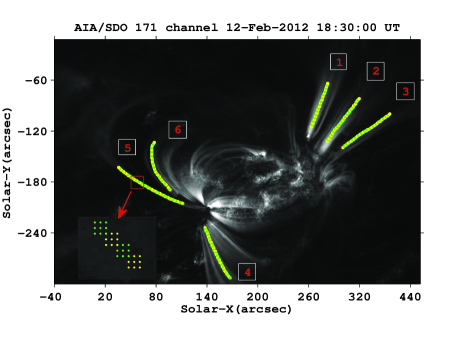
Fig. 1 : A snapshot of the active region (AR11416), observed by AIA/SDO in 171$\rm{\AA}$ on 2012-Feb-12, 18:30 UT. Locations of the selected coronal loop paths that are situated above this active region, are also marked. The coronal loop structures display intensity propagation signal. In order to obtain the intensity as function of distance along loop segments, these paths also are subdivided by successive macropixels with 3$\times$3 pixels wide along the paths. A zoomed in view of a partial segment on loop 1 is shown in the bottom left corner of the Figure.

3 Data Analysis

In order to investigate the oscillatory nature of the intensity propagations along the coronal loop system, the marked regions along the path of the loops are joined by successive macropixels, 3$\times$3 pixels wide along the loop strands. The intensity of each macropixel along the loop system is integrated and divided into the number of pixels at each macropixel. A quasi-static background must be removed from original intensity for enhancing the contrast of intensity variation. Following Yuan and Nakariakov (2012), a background intensity of the form

$$I_{b}(s,t_{n})=\sum_{h=-N/2}^{+N/2-1}I(s,t_{n+h})/N,$$ (1)

is subtracted from time series of intensities, where N is the number of time frames, $t_{n}$ represent the time frame index of the image series ($n=1,~{}t_{1}=0$ corresponds to the first image, $n=2,~{}t_{2}=24s$ corresponds to the second image, …) and $s$ determines the location of macropixels along the indicated paths in Fig. 1 (starting at first sector). An appropriate background constructed from the 100 time frames (48 min) running average in time is subtracted from the original intensities, because a sufficient enhanced time-distance maps is found by setting the $N=100$. It is worth noting that the periods greater than 48 minutes will be suppressed from power spectra of intensities time series by choosing $N=100$.

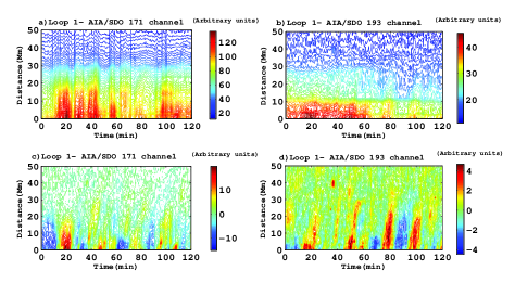
Fig. 2 : Time-distance maps of loop 1 for original intensity (top row), and for background-subtracted intensity (bottom row) are shown in 171 (a) and c) panels) and 193 (b) and d) panels) channels of AIA.

For example, time-distance maps of intensity along the loop 1 for 171$\rm{{\AA}}$ and 193 $\rm{{\AA}}$ before (top panels a) and b)) and after (bottom panels c) and d)) removal of the background intensity are shown in Fig. 2. Intensity as a function of time at each macropixels of six different loop segments which are shown in Fig. 1 is calculated. Also, variation of background-subtracted intensities with time at the 5th macropixel along the loop 1 are shown in the top row panels (a) and b)) of Fig. 3 and, their FFT power spectral densities in the middle row(c) and d)). Also, the period-distance maps are shown in the bottom row panels (e) and f)) for 171$\rm{\AA}$ (left panels), and 193$\rm{\AA}$ (right panels). The Fourier power spectra and period-distance maps of background-subtracted intensity reveal periods in the range of $\rm{P}$ = 8-40 minutes (Fig. 3, middle and bottom row panels). The period-distance maps of intensities show that significance levels ($>0.5$) are in the $\rm{P}=12-35\rm{(min)}$ oscillation periods range. Furthermore, the spectral power densities factor of intensities are dominated at some periods between 12 min and 35 min.

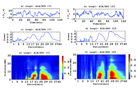
Fig. 3 : The variation of background-subtracted intensities with time at the 5th macropixel along the loop 1 are shown in the top row panels (a) and b)) and, their FFT power spectral densities in the middle row(c) and d)). The Period-distance maps are shown in the bottom row panels for 171$\rm{\AA}$ (left panels), and 193$\rm{\AA}$ (right panels) passbands of AIA/SDO.

4 The method of the physical parameters calculation

Here, the physical parameters of propagating disturbances that are important tools for MHD coronal seismology are extracted with a new method. So, the Fourier components of the intensity time series at each macropixel along the loop structure are multiplied with a Gaussian function of the form

$$a^{{}^{\prime}}_{j}=\sum_{i=1}^{N_{f}}a_{i}\exp[-\frac{(\nu_{i}-\nu_{j})^{2}}{2\sigma^{2}}],$$ (2)

where $N_{f}$ is the number of the Fourier components, $a_{i}$ one of the Fourier components, $a^{{}^{\prime}}_{j}$ one of the interesting dominant component, $\sigma$ standard deviation and $a^{{}^{\prime}}_{i}$ transformed coefficients, respectively (subscript index i and j represent the rank of the harmonics). Also, $\nu_{i}$ and $\nu_{j}$ represent the frequency of the ith and jth harmonics. In the Fourier transformation, the component proportional to the dominant oscillation period is selected by using a Gaussian filter with standard deviation $\sigma\simeq(\nu_{i+1}-\nu_{i-1})/2$ to enhance time-distance maps. For example, Fig. 4 shows the time-distance maps of the loop 1 in 171 Å (left panels) and 193Å (right panels) with the Gaussian filter centered on the dominant oscillation periods of intensity. The time-distance maps of filtered intensities clearly show evidence that acoustic waves propagate upwardly into the coronal loop 1. In the next subsections, the physical parameters of propagating disturbances (slow waves) such as phase speed, damping length, damping time and damping quality are extracted by analyzing the time series of filtered intensities and their enhanced time-distance maps. Furthermore, the results are compared with the previous studies.

4.1 The measurement of the projected phase speed

During the last years several methods are used to determine the speed of a propagating disturbances. Many authors calculated the speed of the propagating disturbances from the gradient of the lines by fitting a linear function to the points with similar amplitude fluctuation of unfiltered time-distance maps. Also, some authors measured the speed of the propagating disturbances by fitting a propagating harmonic wave function to the unfiltered propagating disturbances (see, e.g., De Moortel et al. 2000; Kiddie et al. 2012; Yuan et al. 2012; Threlfall et al. 2013). Here, the time-distance maps of filtered intensities that have periodic features, are used to estimate projected phase speeds of propagating disturbances. For example, Fig. 4 shows the time-distance of the loop 1 in 171 Å (left panels) and 193Å (right panels) with the Gaussian filter centered on the dominant oscillation periods of intensity. The points that have a maximum upward displacement are indicated with red color star signs. The solid blue lines represent a linear function that are fitted to the red star signs, and the gradient of solid lines are used to estimate average projected speeds of propagating disturbances for some particular oscillation periods, also the derived speed for a particular period have been written in the respective panels of Fig. 4. It can be seen that oscillation at a particular period propagates with an almost constant speed along the loop 1 in both passbands. The averages and ranges of observed speeds along the six different paths are compiled in Table 1. The averages and ranges of observed speeds comfortably overlap with previous finding by other authors who analyzed similar observations of propagating fluctuations (see, e.g., De Moortel et al. 2000; Marsh et al. 2003, 2009; Kiddie et al. 2012; Yuan et al. 2012; Threlfall et al. 2013; Sych and Nakariakov, 2014). This method has several advantages. (1) The time-distance maps of filtered intensities clearly show evidence that acoustic waves propagate upwardly into coronal loops (see Fig.4). (2) To distinguish the points with maximum displacement (or points with similar displacement) from these maps is very much easier than the time-distance maps of unfiltered intensities, then this method can produce reliable results. (3) Furthermore, this method reveals how the magnitude of physical parameters vary depending on the oscillation periods.

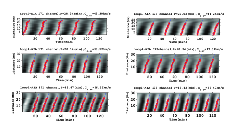
Fig. 4 : Quasi-periodic longitudinal features along the loop1 in 171 (left panels) and 193 (right panels) channels of AIA. The location of the points that have a maximum upward displacement are indicated with red color $\ast$ signs. The solid blue lines represent a linear function that are fitted to the red star signs, and the gradient of the solid lines in each panel are used to estimate average projected speed along loop 1 at a particular period.

4.2 The measurement of damping of slow waves and the dependence of damping value on its frequency

Damping of MHD waves have been studied extensively in coronal structures both theoretically and observationally since their first detection. However, studies on the dependence of damping value on its frequency are limited. Fourier power spectral densities of background-subtracted intensities show that Fourier components of the intensity time series at each macropixel along the six different paths are only significant at some specified period in the range of $\rm{P}=10-35$ minutes. For example, the period-distance maps constructed for loop 1 in the 171 (bottom left panel) and 193 Å (bottom right panel), are shown in the Fig. 3. To estimate the damping length of MHD waves and the dependence of damping length on its frequency, the amplitude at a particular period in the range of $\rm{P}=12-35$ minutes is measured by taking the square root of its power component. The amplitude decay of filtered intensities at a certain period as function of distance along the six paths of Fig. 1 is fitted with an exponential function of the form

$$A(s)=A_{0}exp(-\gamma_{d}s)+C_{0},$$ (3)

where, $\gamma_{d}$ is the damping length coefficient, $A_{0}$ and $C_{0}$ appropriate constant. The projected damping length ($\rm{L_{d}}=1/\gamma_{d}$) of filtered intensity is calculated by Matlab Statistics Toolbox  Curve Fitting and Distribution Fitting. Figure 5 shows a typical example of the amplitude decay of oscillations as a function of distance along loop 1 (blue star signs) with $\rm{P}=28.43,~{}27.03,~{}20.14,~{}20.34,~{}13.14$ and $13.42~{}\rm{min}$ that an exponential function is fitted to the data (red lines) in both passbands (171 and 193 Å). The fitting parameters are written in the top of panels. Also, in order to compare the dependence of damping length on its periodicity in Fig. 5, the amplitude at each period is normalized to the amplitude of a segment along the path that oscillate with maximum amplitude. Amplitude decay lengths of oscillation as a function of period are shown for all six different paths in Fig. 6. These results indicate that the projected damping lengths are in the range of 23 Mm to 68 Mm for periods in the rage between 12 and 35 min. The observed physical parameters such as oscillation period $\rm{P}$, phase speed $\rm{C_{s}}$, damping length ($\rm{L_{d}}$), damping time ($\rm{\tau_{d}=L_{d,est}/C_{s}}$) and damping quality ($\rm{\tau_{d}/P}$), for filtered oscillation part of intensity at a sequence of 300 images with 24 s time intervals are listed in Table1 for six different loop segments. The results of data analysis indicate that magnitude of phase speed and damping time along the six different loop segments are in the range of $38-79~{}\rm{km~{}s^{-1}}$ and $\rm{\tau_{d}}\simeq 7-21~{}\rm{min}$, respectively. The magnitudes of damping quality for dominant oscillation periods in the six loop segments are in the range of $\rm{\tau_{d}/P}\simeq 0.35-0.77$ which clearly show that damping regime is strong for dominant oscillation periods.

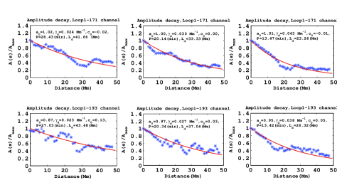
Fig. 5 : Typical examples of the normalized amplitude decay profiles $A(s)/A_{max}$ for loop 1 at $\rm{P}=28.43,~{}27.03,~{}20.14,~{}20.34,~{}13.14$ and $13.42~{}\rm{min}$ are shown as function of the projected distance. The data is fitted by an exponential function, $A(s)/A_{max}=a_{0}\exp(-\gamma_{d}s)+c_{0}$ (red lines), and fit parameters are written in the top of the panels. Top and bottom panels correspond to the data from 171 and 193 channels respectively.

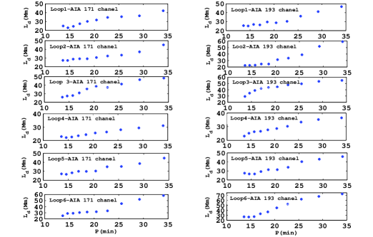
Fig. 6 : Variation of observed damping lengths $\rm{L_{d}}$ with period in 171 (left panels) and 193 (right panels) channels of AIA for 6 loop segments marked in the panel of Fig. 1.

Table 1 : Averages and ranges of physical parameters, such as periodicity, projected damping length, projected propagation speeds, damping time ($\rm{\tau_{d}=L_{d}/C_{s.av}}$), and damping quality (damping time per period, $\rm{\tau_{d}/P}$) of 6 paths along the coronal loops observed with AIA/SDO 171 and 193 Å passbands.

	Loop 1
$\rm{Band}(\rm{\AA})$	$\rm{P}(min)$	$\rm{C_{s}(km~{}s^{-1})}$			$\rm{L_{d}(Mm)}$	$\rm{\tau_{d}(min)}$	$\rm{\tau_{d}/P}$
		$\rm{.min}$	$\rm{.max}$	$\rm{.av}$
	28.43	39.88	44.95	42.30	41.55	16.37	0.58
171	20.14	54.97	64.51	58.52	33.31	9.48	0.47
	13.47	45.18	47.72	46.55	23.45	8.40	0.62
	27.03	38.48	44.99	41.25	43.65	17.63	0.65
193	20.34	47.10	49.65	47.51	36.72	12.88	0.63
	13.42	55.55	61.69	58.40	26.34	7.52	0.52
	Loop 2
	25.56	39.88	44.95	42.30	35.08	13.82	0.49
171	20.54	48.14	53.86	50.40	32.16	10.63	0.53
	15.73	46.47	50.51	48.60	27.14	9.31	0.69
	25.61	38.48	39.99	39.36	39.12	16.56	0.61
193	20.52	48.24	31.25	49.28	31.32	10.60	0.52
	15.63	45.92	50.91	48.11	23.54	8.15	0.56
	Loop 3
	29.44	37.66	46.33	42.04	46.34	18.37	0.62
171	18.59	47.15	52.40	50.33	35.58	12.77	0.69
	-	-	-	-	-	-	-
	30.21	37.6	46.30	41.90	53.05	21.10	0.69
193	18.74	47.06	53.03	50.01	43.46	14.48	0.77
	-	-	-	-	-	-	-
	Loop 4
	29.20	51.28	57.96	53.95	33.46	10.34	0.35
171	25.56	44.67	48.96	46.68	28.03	10.01	0.39
	17.04	64.36	75.02	67.57	23.60	5.82	0.34
	29.20	39.27	42.89	41.12	35.15	14.25	0.49
193	22.71	44.08	50.31	46.61	30.21	10.80	0.47
	17.04	50.12	55.48	52.63	26.56	8.41	0.49
	Loop 5
	34.07	51.12	51.86	51.52	44.61	14.43	0.42
171	25.56	59.49	70.04	64.58	35.28	9.08	0.35
	20.44	40.70	47.79	44.82	30.19	11.23	0.55
	34.07	43.43	44.72	44.29	45.91	17.28	0.50
193	25.56	40.67	53.71	43.92	40.28	15.28	0.59
	20.44	36.78	40.83	38.44	31.43	13.62	0.66
	Loop 6
	29.20	47.11	22.98	59.88	52.03	14.48	0.49
171	25.44	74.09	82.87	78.99	44.10	9.30	0.36
	20.02	60.30	64.68	62.68	31.71	8.43	0.42
	30.07	72.88	82.94	77.72	67.50	15.57	0.53
193	25.56	72.29	80.47	77.29	62.45	13.46	0.52
	20.44	58.18	72.53	63.14	27.12	7.15	0.35

5 Theoretical considerations

Theoretical studies investigating the damping of the slow wave have concentrated on the effects of thermal conduction, compressive viscosity, optically thin radiation, gravitational stratification and magnetic field divergence. Generally, thermal conduction is found to be the dominant mechanism for dissipation of slow modes in the solar corona (De Moortel and Hood, 2003, 2004a, 2009; Pandey and Dwivedi 2006; Ofman and Wang, 2002; Van Doorsselaere et al. 2011; Abedini et al. 2012). Here, the coronal loops are considered a homogeneous plasma medium in the presence of thermal conduction, compressive viscosity and optically thin radiation dissipation mechanism with constant equilibrium values $\rho_{0}$, $\rm{T_{0}}$, $p_{0}$ and no flow ($v_{0}=0$), also with a uniform background magnetic field along the loops. Assuming all disturbances in terms of Fourier components for frequency ($\omega$) and wave number ($k$) in z-direction, $\exp i(kz-\omega t)$, combining linearized MHD equations in the presence of thermal conduction $(E_{c}=\frac{\partial}{\partial z}(k_{||}\frac{\partial\rm{T_{0}}}{\partial z}))$, compressive viscosity $(E_{\eta}=\frac{4}{3}\eta_{0}(\frac{\partial v}{\partial z})^{2})$ and optically thin radiation $(E_{r}=\chi\rm{n_{e}^{2}}\rm{T_{0}}^{\alpha})$ (Sigalotti et al. 2007) leads to the following dispersion relation:

$$i{\cal A}k^{4}+i{\cal B}k^{2}+i{\cal C}=0,$$ (4)

$${\cal A}=-(\gamma-1)k_{||}[\frac{4}{3}\frac{\eta_{0}\rm{T_{0}}}{\rho_{0}p_{0}}\omega+\frac{\rm{T_{0}}}{\rho_{0}}],$$

$${\cal B}=(\gamma-1)[k_{||}\frac{\rm{T_{0}}}{p_{0}}\omega^{2}+\frac{4}{3}\frac{\eta_{0}}{\rho_{0}}+i\omega\frac{\gamma p_{0}}{\rho_{0}},$$

$$~{}~{}~{}~{}~{}+\chi(i\omega\frac{4}{3}\alpha\frac{\eta_{0}}{p_{0}}-\alpha+2)\frac{\rho_{0}\rm{T_{0}}^{\alpha}}{\overline{m}^{2}}],$$

$${\cal C}=\omega^{2}[\alpha\chi(\gamma-1)\frac{\rho_{0}^{2}\rm{T_{0}^{\alpha}}}{\overline{m}^{2}p_{0}}-i\omega],$$

Here, $\gamma=5/3$, $\overline{m}=0.6m_{H}$, $\eta_{0}=10^{-17}T_{0}^{5/2}\rm{kgm^{-1}s^{-1}}$, $k_{||}=10^{-11}\rm{T_{0}^{5/2}}~{}\rm{Wm^{-1}K^{-1}}$ are taken and $\chi$ and $\alpha$ are temperature dependent ( Braginskii, 1965; Hildner, 1974). Furthermore, the $\omega$ is assumed to be real and the wave number is imaginary ($k=k_{r}+ik_{i}$). The measured propagation speed of the intensity disturbances is a projected component of sound speed which is perpendicular to the LOS (line-of-sight). By analyzing the filtered intensity with particular periods in the range of ($8-40~{}\rm{min})$, the average value of projected sound speed along the selected paths was found in the range of $38-79~{}\rm{km~{}s^{-1}}$. So, it can be concluded that average value of real sound speed is greater than $38~{}\rm{km~{}s^{-1}}$. The temperature associated with $\rm{C_{s}}=38~{}\rm{km~{}s^{-1}}$ is found $0.1~{}\rm{MK}$ by using the theoretical relation $T_{0}=\frac{\overline{m}C_{s}^{2}}{\gamma k_{B}}$, and by inserting the Boltzmann constant $k_{B}=1.38\times 10^{-23}~{}\rm{JK^{-1}}$. In a propagating wave with a specific oscillation period $\rm{P}$ that has a damping length $\rm{L_{d}}$, it is expected to have $\rm{P}=2\pi/(k_{r}\rm{C_{s}})$, and $\rm{L_{d}}=1/k_{i}$. In order to estimate damping length, the wave number of propagation wave associated with oscillation period ($5-40\rm{min}$) at different values of temperature ($\rm{T_{0}=0.1,~{}0.5,~{}1,~{}1.5,~{}and`~{}2~{}\rm{MK}}$) is calculated based on numerical solutions of dispersion relation (4). Plot of $2\pi/(k_{r}\rm{C_{s}})$ in (min) (top panels) and the estimated damping length $\rm{L_{d,est}}=1/k_{i}$ in Mm (bottom panels), as a function of $(\rm{log(n_{e}/n_{0}),~{}n_{0}=10^{4}~{}cm^{-3}})$ due to the presence of combining dissipation mechanism are shown in Fig. 7 for different values of temperature and oscillation period. In each panel of Fig. 7, acceptable range ($2\pi/(k_{r}\rm{C_{s})=5,~{}10,~{}15,~{}20,~{}25,~{}30,~{}35~{}and~{}40}$ min) of damping length and number density are outlined with blue rectangle. An interesting prediction of this model is that the plots of $\rm{L_{d,est}}$ as a function of $(\rm{log(n_{e}/n_{0})})$ have a maximum in acceptable range. Another interesting feature visible in these plots is that both damping lengths and their maximum value increase with increasing $\rm{T_{0}}$ and $\rm{P}$. Also, the maximum point of $\rm{L_{d,est}}$ shifts toward bigger electron number density. These results reveal that treatment of estimated damping due to the presence of dissipation mechanism is complex and its value depends not only on the oscillation period but also on the electron number density and temperature. Moreover, the results based on numerical solutions of dispersion relation illustrate that, although the damping length and damping time can be increased with increasing the oscillation periods, the dependence on periodicity and value of these quantities strongly depend on the temperature and the electron number density.

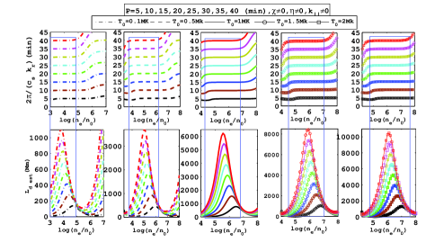
Fig. 7 : Plot of the the estimated damping length $\rm{L_{d,est}}$ in Mm (bottom), and $2\pi/(k_{r}\rm{C_{s}})$ in min as a function of the dimensionless electron number density $(\rm{log(n_{e}/n_{0}),~{}n_{0}=10^{4}cm^{-3}})$ (top) due to the presence of all three dissipation mechanisms for different temperatures $\rm{T_{0}=0.1,0.5,1,1.5~{}and~{}2}$ MK and periods $\rm{P=5,10,15,20,25,30,35~{}and~{}40}$ min in the acceptable range. The acceptable range of damping length and number density are outlined with blue rectangle in the panels.

Table 2 : Ranges of physical parameters such as estimated damping length ($\rm{L_{d,est}=1/k_{i}}$), damping time ($\rm{\tau_{d}=L_{d,est}/C_{s}}$ ), damping quality ($\rm{\tau_{d,est}/P}$) and electron number density within the acceptable regions ( $2\pi/(k_{r}\rm{C_{s})=5,10,...,35,~{}and~{}40}$ min) are calculated at dominant oscillation periods for different values of temperature ($\rm{T_{0}=0.1,0.5,1,1.5~{}and~{}2~{}\rm{MK}}$).

$\rm{T_{0}(MK)}$	$\alpha$	$\chi$	P(min)	$\chi\neq 0,\eta\neq 0,k_{||}\neq 0$
				$\rm{log(n_{e}/n_{0})}$	$\rm{L_{d,est}(Mm)}$	$\rm{\tau_{d,est}(min)}$	$\rm{\tau_{d,est}/P}$
				Range	Range	Range	Range
			5	3-5.8	$\geq 9$	$\geq 4$	$\geq 0.66$
			10	3-5.6	$\geq 19$	$\geq 8.5$	$\geq 0.72$
			15	3-5.4	$\geq 48$	$\geq 20.5$	$\geq 1.16$
0.1	0	$8\times 10^{-34}$	20	3-5.1	$\geq 80$	$\geq 35$	$\geq 1.49$
			25	3-5	$\geq 134$	$\geq 54.5$	$\geq 1.85$
			30	3-4.95	$\geq 180$	$\geq 78$	$\geq 2.22$
			35	3-4.85	$\geq 230$	$\geq 97$	$\geq 2.36$
			40	3-4.75	$\geq 332$	$\geq 138$	$\geq 2.93$
			5	3.4-7.8	$\geq 18$	$\geq 3$	$\geq 0.56$
			10	3.4-7.6	$\geq 36$	$\geq 6$	$\geq 0.58$
			15	3.4-7.4	$\geq 58$	$\geq 8.9$	$\geq 0.59$
0.5	-2.5	$3.94\times 10^{-21}$	20	3.4-7	$\geq 76$	$\geq 12$	$\geq 0.6$
			25	3.4-6.8	$\geq 150$	$\geq 24.5$	$\geq 0.93$
			30	3.4-6.6	$\geq 221$	$\geq 36$	$\geq 1.14$
			35	3.4-6.4	$\geq 332$	$\geq 54$	$\geq 1.47$
			40	3.4-6.25	$\geq 385$	$\geq 63$	$\geq 1.49$
			5	4.7-8.2	$\geq 25$	$\geq 2.75$	$\geq 0.53$
			10	4.6-8	$\geq 50$	$\geq 5.54$	$\geq 0.53$
			15	4.5-7.8	$\geq 80$	$\geq 8.86$	$\geq 0.57$
1	-1	$5.51\times 10^{-30}$	20	4.4-7.5	$\geq 130$	$\geq 14.4$	$\geq 0.69$
			25	4.3-7.3	$\geq 210$	$\geq 23.25$	$\geq 0.89$
			30	4.25-7.1	$\geq 320$	$\geq 35.43$	$\geq 1.13$
			35	4.2-6.95	$\geq 380$	$\geq 42.08$	$\geq 1.15$
			40	4.25-6.75	$\geq 540$	$\geq 59.79$	$\geq 1.43$
			5	5-8	$\geq 30$	$\geq 2.7$	$\geq 0.52$
			10	4.8-8	$\geq 62$	$\geq 5.6$	$\geq 0.54$
			15	4.6-8	$\geq 126$	$\geq 11.4$	$\geq 0.73$
1.5	-1	$5.51\times 10^{-30}$	20	4.5-7.8	$\geq 158$	$\geq 14.3$	$\geq 0.69$
			25	4.7-7.6	$\geq 240$	$\geq 21.7$	$\geq 0.83$
			30	4.6-7.4	$\geq 360$	$\geq 32.6$	$\geq 1$
			35	4.5-7.2	$\geq 406$	$\geq 36.7$	$\geq 1$
			40	4.4-7	$\geq 590$	$\geq 53.4$	$\geq 1.3$
			5	5.2-8	$\geq 37$	$\geq 2.89$	$\geq 0.55$
			10	5-8	$\geq 71$	$\geq 5.54$	$\geq 0.53$
			15	4.8-8	$\geq 112$	$\geq 8.74$	$\geq 0.56$
2	-1	$5.51\times 10^{-30}$	20	4.4-8	$\geq 180$	$\geq 14$	$\geq 0.67$
			25	4.8-8	$\geq 350$	$\geq 27.3$	$\geq 1$
			30	4.8-8	$\geq 440$	$\geq 34.32$	$\geq 1$
			35	4.8-7.8	$\geq 532$	$\geq 41.5$	$\geq 1.14$
			40	4.75-7.6	$\geq 610$	$\geq 47.58$	$\geq 1.14$

6 Discussion and Conclusions

The aim of this paper is to study the physical parameters of longitudinal intensity variations in the large active-region loop systems by AIA/SDO. So, 300 high cadence images of loop systems with an interval of 24 seconds in the 171$\rm{\AA}$ and 193 $\rm{\AA}$ are analyzed. First, the intensity as a function of distance along the six loop segments is calculated for all times. Then a background constructed from the 100 point (40 min) running average in time is subtracted from the original intensities. For example, the time-distance maps of intensity along the loop 1 before (panels a) and b )) and after (panels c) and d)) removal of the background intensity are shown in top and bottom rows of Fig. 2, respectively. The Fourier power spectra and period-distance map of fluctuating part of intensities along the loop segments reveal periods in the range of $\rm{P}\simeq 8-40$ minutes for both the AIA channels (for example, see the middle and bottom rows of Fig. 2). Moreover, the filtered fluctuating intensity of loops shows small amplitude periodic variations which are interpreted as evidence for damping of slow magneto-acoustic waves in loop systems (see bottom panels in Fig. 2 and Fig. 4). This range of oscillation period that has been estimated in this study comfortably overlaps with values quoted by other authors who analyzed similar observations of propagating fluctuations and MHD theory’s predictions for the slow wave (see, e.g., De Moortel et al. 2002, 2003, 2004; Marsh et al. 2003, 2004, 2009, 2011; Krishna et al. 2014, Yuan and Nakariakov 2012, Kiddie et al. 2012). Time-distance images formed from the integrated intensity along the loop segments show that disturbances propagate approximately with a constant speed. Accordingly, the projected speeds of filtered intensity along the 6 loop segments are estimated for some dominant oscillation period between 12 min and 35 min, by fitting a linear function to the points with maximum amplitude fluctuation of time-distance maps. Also, the damping length ($\rm{L_{d}}$) of oscillation are calculated by fitting an exponentially decreasing function to the filtered fluctuation part of intensity profiles (see Fig. 5). Other physical parameters, such as damping time ($\rm{\tau_{d}=L_{d}/C_{s.av}}$) and damping quality ($\rm{\tau_{d}/P}$), are calculated by using the speeds and damping lengths. The some results of analysis in the 171 Å and 193 Å passbands are listed in Table 1 for different loop segments. These observed results show that:

• The average values of projected speeds for dominant oscillation periods of six different loop segments are in the range of $38-79~{}\rm{km~{}s^{-1}}$.

• The average values of damping lengths and damping times are in the range of $23-68~{}\rm{Mm}$ and $7-21~{}\rm{min}$, respectively. Also, its values are sensitive to the oscillation period and increase with increasing $\rm{T_{0}}$ and $\rm{P}$.

• The magnitude value of damping qualities are obtained in the range of $<1$ for filtered intensity which correspond to strong damping regime.

Also, to compare observed results with the theoretical MHD prediction, the estimated physical parameters of the slow wave that has concentrated on the effects of thermal conduction, compressive viscosity and optically thin radiation is investigated. The damping lengths of filtered intensities as function of electron number density based on the theoretical MHD prediction are shown in Fig. 7 for different values of temperature ($\rm{T_{0}=0.1,~{}0.5,~{}1.5~{}and~{}2~{}\rm{MK}}$). The magnitudes of estimated damping lengths and other physical parameters in the acceptable range ($2\pi/(\rm{C_{s}}k_{r})\simeq\rm{5,10,...,35,~{}and~{}40~{}\rm{min}}$) are listed in Table 2. These results show that:

• In the presence of three dissipation mechanisms together damping lengths and damping times increase with increasing temperature and oscillation period but damping qualities decrease with increasing temperature (see Table 2)

• The plots of damping length as function of electron number density have a maximum in acceptable range (see Fig. 7).

• The damping lengths and their maximum value increase with increasing $\rm{T_{0}}$ and $\rm{P}$. Also, the maximum point of plots shift toward bigger electron number density.

• The dependence on periodicity and value of damping length strongly depend on the temperature and the electron number density. These theoretical results reveal that treatment of estimated damping due to the presence of all three dissipation mechanisms is complex and its value depends not only on the oscillation period but also on the electron number density and temperature.

The magnitudes of observed damping times and damping qualities are independent of the LOS. comparing the observed damping times and dependence of damping times on their periods with the theoretically predicted values, it can be seen at low periods ($\rm{P}<15~{}\rm{min}$), the damping times and the dependence of damping times on their periods of propagating slow magneto-acoustic waves in the gravitationally stratified loops that are situated above active regions may be explained by considering three dissipation mechanisms in an especial range of electron number density ($\rm{n_{e}}\simeq 10^{7}-10^{12}~{}\rm{cm^{-3}}$) but at high periods the other dissipation mechanism must be considered. Also, It can be concluded that the behavior of propagating slow magneto-acoustic waves along the corona loops, in addition to the dispersion mechanism, can depend on the other quantities such as temperature, electron number density, and so on.

References

- Abedini (2011) Abedini, A., Safari, H.: New Astron., 16, 317 (2011)
- Abedini (2012) Abedini, A., Safari, H., Nasiri, S.: Sol. Phys., 280, 137 (2012)
- Banerjee (2007) Banerjee, D., Erdélyi, R., Oliver, R., Óshea, E.: Sol. Phys., 246, 3 (2007)
- Braginskii (1965) Braginskii, S.I.: Rev, Plasma Phys., 1, 205 (1965)
- Berghmans (1999) Berghmans, D., Clette, F.: Sol. Phys., 186, 207 (1999)
- Deforest (1998) DeForest, C.E., Gurman, J.B.: Astrophys. J., 501, L217 (1998)
- DeMoortel (2000) De Moortel, I., Ireland, J., Walsh, R.W.: Astron. Astrophys., 355, L23 (2000)
- DeMoortel (2002) De Moortel, I., Ireland, J., Walsh, R.W., Hood, A.W.: Sol. Phys., 209, 61 (2002)
- DeMoortel (2003) De Moortel, I., Hood, A.W.: Astron. Astrophys., 408, 755 (2003)
- DeMoortel (2004a) De Moortel, I., Hood, A.W.: Astron. Astrophys., 415, 705 (2004a)
- DeMoortel (2004) De Moortel, I., Hood, A.W., De Pontieu, B.: ESASP, 547, 427 (2004)
- DeMoortel (2009) De Moortel, I.: Space Sci. Rev., 149, 65 (2009)
- Erdelyi (2008) Erdélyi, R., Luna-Cardozo, M., Mendoza-Briceño, C.A.: Sol. Phys., 252, 305 (2008)
- Hildner (1974) Hildner, E.: Sol. Phys., 35, 123 (1974)
- Kiddie (2012) Kiddie, G., De Moortel, I., Del Zanna, G., McIntosh, S.W., Whittaker, I.: Sol. Phys., 279, 427 (2012)
- Klime (2002) Kliem, B., Dammasch, I.E., Curdt, W., Wilhelm, K.: Astrophys. J., 568, L61 (2002)
- Klimchuk (2004) Klimchuk, J.A., Tanner, S.E.M., De Moortel, I.: Astrophys. J., 616, 1232 (2004)
- Krishna (2014) Krishna Prasad, S., Banerjee, D., Van Doorsselaere, T.: Astrophys. J., 789, 118 (2014)
- Mariska (2006) Mariska, J.T.: Astrophys. J., 639, 484 (2006)
- Mariska (2010) Mariska, J.T., Muglach, K.: Astrophys. J., 713, 573 (2010)
- Marsh (2003) Marsh, M.S., Walsh, R.W., De Moortel, I., Ireland, J.: Astron. Astrophys., 404, L37 (2003)
- Marsh (2004) Marsh, M.S., Walsh, R.W., De Moortel, I., Ireland, J.: ESASP., 547, 519 (2004)
- Marshw (2009) Marsh, M.S., Walsh, R.W., Plunkett, S.: Astrophys. J., 697, L1674 (2009)
- Marsh2011 (2011) Marsh, M.S., De Moortel, I., Walsh, R.W.: Astrophys. J., 734, 81 (2011)
- McEwan (2006) McEwan, M.P., De Moortel, I.: Astron. Astrophys., 448, 763 (2006)
- Mendoza (2004) Mendoza-Briceño, C.A., Erdélyi, R., Sigalotti, L., Di, G.: Astrophys. J., 605, 493 (2004)
- Nakariakov (2000) Nakariakov, V.M., Verwichte, E., Berghmans, D., Robbrecht, E.: Astron. Astrophys., 362, 1151 (2000)
- Nakariakov (2005) Nakariakov, V.M., Verwichte, E.: LRSP, 2, 3 (2005)
- Ofman (1997) Ofman, L., Romoli, M., Poletto, G., Noci, G., Kohl, J.L.: Astrophys. J., 491, L111 (1997)
- Ofman (1999) Ofman, L., Nakariakov, V.M., DeForest, C.E.: Astrophys. J., 514, 441 (1999)
- Ofman (2000) Ofman, L., Nakariakov, V.M., Sehgal, N.: Astrophys. J., 533, 1071 (2000)
- Ofman (2002) Ofman, L., Wang, T.J.: Astrophys. J., 580, L85 (2002)
- pendy (2006) Pandey, V.S., Dwivedi, B.N.: Sol. Phys., 236, 127 (2006)
- porter (1994) Porter, L.J., Klimchuk, J.A., Sturrock, P.A.: Astrophys. J., 435, 502 (1994)
- Roberts (2000) Roberts, B.: Sol. Phys., 193, 139 (2000)
- Roberts (2006) Roberts, B.: RSPTA., 364, 447 (2006)
- Sakurai (2002) Sakurai, T., Ichimoto, K., Raju, K.P., Singh, J.: Sol. Phys., 209, 265 (2002)
- Sigalotti (2007) Sigalotti, L., Di, G., Mendoza-Briceño, C.A., Luna-Cardozo, M.: Sol. Phys., 246, 187 (2007)
- Sych (2014) Sych, R., Nakariakov, V. M.: Astron. Astrophys., 569, A72 (2014)
- Threlfall2013 (2013) Threlfall, J., De Moortel, I., McIntosh, S.W., Bethge, C.: Astron. Astrophys., 556, A124 (2013)
- Tsiklauri (2001) Tsiklauri, D., Nakariakov, V.M.: Astron. Astrophys., 379, 1106 (2001)
- Uchida (1968) Uchida, Y.: Sol. Phys., 4, 30 (1968)
- Uchida (1970) Uchida, Y.: PASJ., 22, 341 (1970)
- Uritsky (2013) Uritsky, V.M., Davila, J.M., Viall, N.M., Ofman, L.: Astrophys. J., 778, 26 (2013)
- VanDoorsselaere (2011) Van Doorsselaere, T., Wardle, N., Del Zanna, G., Jansari, K., Verwichte, E., Nakariakov, V.M.: Astrophys. J., 727, L32 (2011)
- Verwichte (2005) Verwichte, E., Nakariakov, V.M., Cooper, F.C.: Astron. Astrophys., 430, L65 (2005)
- Verwichte (2008) Verwichte, E., Haynes, M., Arber, T.D., Brady, C.S.: Astrophys. J., 685, 1286 (2008)
- Wang (2002a) Wang, T.J., Solanki, S.K., Curdt, W., Innes, D.E., Dammasch, I.E.: Astrophys. J., 574, L101 (2002a)
- Wang (2002c) Wang, T.J., Solanki, S.K., Curdt, W., Innes, D.E., Dammasch, I.E.: ESASP., 505, 199 (2002c)
- Wang (2003a) Wang, T.J., Solanki, S.K., Innes, D.E., Curdt, W., Marsch, E.: Astron. Astrophys., 402, L17 (2003a)
- Wang (2003b) Wang, T.J., Solanki, S.K., Curdt, W., Innes, D.E., Dammasch, I.E., Kliem, B.: Astron. Astrophys., 406, 1105 (Paper I) (2003b)
- Wang (2009) Wang, T.J., Ofman, L., Davila, J.M., Mariska, J.T.: Astron. Astrophys., 503, L25 (2009)
- Wang (2011) Wang, T.J.: Space Sci. Rev., 158, 397 (2011)
- Yuan (2012) Yuan, D., Nakariakov, V.M.: Astron. Astrophys., 543, A9 (2012)