Phase transitions and ordering structures of a model of chiral helimagnet
in three dimensions

Abstract

Phase transitions in a classical Heisenberg spin model of a chiral helimagnet with the Dzyaloshinskii–Moriya (DM) interaction in three dimensions are numerically studied. By using the event-chain Monte Carlo algorithm recently developed for particle and continuous spin systems, we perform equilibrium Monte Carlo simulations for large systems up to about $10^{6}$ spins. Without magnetic fields, the system undergoes a continuous phase transition with critical exponents of the three-dimensional XY model, and a uniaxial periodic helical structure emerges in the low temperature region. In the presence of a magnetic field perpendicular to the axis of the helical structure, it is found that there exists a critical point on the temperature and magnetic-field phase diagram and that above the critical point the system exhibits a phase transition with strong divergence of the specific heat and the uniform magnetic susceptibility.

I Introduction

Frustration and competition between interactions and/or fields often induce complicated spin structures into magnetic materials such as spin ice, magnetic skyrmion, and spin liquid. Phase transitions and phase diagrams in magnetic materials driven by various interactions and fields have been extensively studied in condensed matter physics and also statistical physics. Among them, chiral magnets such as MnSi have recently attracted great interests to experimental and theoretical studies not only for its fundamental properties but also for applications Kishine et al. (2005); Togawa et al. (2012, 2013); Ghimire et al. (2013); Zhang et al. (2015); Dzyaloshinskii (1964a, b, 1965); Kishine et al. (2014). Chiral helimagnet is a magnetic system in which a uniaxial helical structure emerges in the low temperature region. The helical structure is induced by the Dzyaloshinskii–Moriya (DM) interaction Dzyaloshinsky (1958); Moriya (1960) which is an antisymmetric interaction breaking a chiral symmetry, and thus, the two same helical structures with different winding directions do not degenerate. By a variational analysis of a one-dimensional continuum model Dzyaloshinskii (1964a, b, 1965); Kishine et al. (2014), it is revealed theoretically that a chiral magnetic soliton lattice (CSL) is formed with a finite magnetic field perpendicular to the axis of the helical structure, and a continuous phase transition to forced ferromagnetic phase occurs with increasing the magnetic field. A mean-field analysis shows that a phase transition into the CSL phase occurs at a finite temperature under the magnetic field Shinozaki et al. (2015).

While recent experiments Togawa et al. (2012, 2013) have reported the existence of the CSL state at finite temperatures in three dimensions, finite-dimensional effects beyond the mean-field theory on the nature of the finite-temperature phase transitions of the system are still less clear. In the absence of magnetic fields, renormalization-group approaches Liu (1973); Klein and Aharony (1991) predict that the system undergoes a continuous phase transition with critical exponents of the ferromagnetic XY model. Another theoretical study Calvo (1981) also indicates that the system belongs to the same universality class of the ferromagnetic XY model. On the other hand, with the magnetic field perpendicular to the axis of the helical structure, the system no longer has any continuous symmetry in the spin space. Therefore, the nature of a possible phase transition in three dimensions is nontrivial and possibly different from the three-dimensional XY model.

In this paper, we study a three-dimensional classical Heisenberg spin model of a chiral helimagnet by equilibrium Monte Carlo simulations. We especially focus on its phase transitions and ordering structures in the low temperature region with and without the magnetic field. Because of the competition among the DM interaction, the symmetric exchange interaction, and the magnetic field, complicated ordering structures emerge in the low temperature region. In particular, there are many CSL states with different numbers of chiral solitons which are separated with each other by large energy barrier. Hence, a transition between the different CSL states hardly occurs by means of conventional Monte Carlo algorithms such as the Metropolis and the heat-bath algorithm. In order to reduce the difficulty of the slow relaxation, we use the event-chain Monte Carlo algorithm Bernard et al. (2009); Peters and de With (2012); Michel et al. (2014, 2015); Nishikawa et al. (2015) which is a recently proposed rejection-free and efficient algorithm for equilibrium simulations. This algorithm enables us to equilibrate quite large systems with more than $10^{6}$ spins so as to avoid suffering from its strong finite-size effects particularly in the presence of the magnetic field.

This paper is organized as follows. In Section II we define a classical Heisenberg spin model of a chiral helimagnet and various physical quantities. The details of the event-chain Monte Carlo algorithm are presented in Section III. In Section IV, results of our Monte Carlo simulations are shown, and properties of phase transitions and ordering structures of the system with and without a magnetic field are discussed. In Section V we discuss a possible phase diagram and summarize our results.

II Model and physical quantities

In this paper, we study a classical Heisenberg model of a chiral helimagnet in a three-dimensional simple cuboidal lattice. The system is defined by the Hamiltonian

$$H\left(\left\{\boldsymbol{S}_{i}\right\}\right) = -J\sum_{\left\langle i,j\right\rangle}\boldsymbol{S}_{i}\cdot\boldsymbol{S}_{j}-\boldsymbol{D}\cdot\sum_{i}\left(\boldsymbol{S}_{i}\times\boldsymbol{S}_{i+\hat{y}}\right)$$ (1)

$$\hskip 85.35826pt-\boldsymbol{h}\cdot\sum_{i}\boldsymbol{S}_{i},$$

where $\boldsymbol{S}_{i}$ is a unit vector with three components, $J$ is a positive coupling constant, $\boldsymbol{D}=D\hat{y}$ is the DM vector, and $\boldsymbol{h}=h\hat{z}$ is a magnetic field perpendicular to the DM vector $\boldsymbol{D}$. The summation in the first term runs over all the neighboring pairs of sites, and the other summations run over all the sites. The lattice on which the system is defined is a cuboid where the linear size of $y$ direction is $\alpha$ times as long as $x$ and $z$ directions. The linear size of $x$ and $z$ directions of the lattice is denoted by $L$ and the total number of sites is $N=\alpha L^{3}$. We set $\alpha=8$ in the following of this paper. Periodic boundary conditions are imposed on $x$ and $z$ directions and a free boundary condition on $y$ direction.

The second term in the Hamiltonian (1) represents the Dzyaloshinskii–Moriya interaction Dzyaloshinsky (1958); Moriya (1960) which induces a helical spin structure. In the ground state of the system without magnetic fields, all spins in each $x$-$z$ plane align ferromagnetically and the spins in each plane make a canted angle $\theta=\arctan(D/J)$ with respect to its nearest neighbor plane along the DM vector. The wave vector $\boldsymbol{q}_{\mathrm{chiral}}$ corresponding to the helical structure in the ground state is determined by $D/J$ via

$$\boldsymbol{q}_{\mathrm{chiral}}=\arctan\left(\frac{D}{J}\right)\hat{y}.$$ (2)

At a finite temperature, the system undergoes a phase transition from a paramagnetic phase to a chiral helimagnetic phase as temperature decreases. Following the work by Calvo Calvo (1981), the system without magnetic fields can be exactly mapped onto another system defined by the Hamiltonian

$$H^{\prime}\left(\left\{\boldsymbol{S}_{i}\right\}\right)=-J\sum_{\left\langle i,j\right\rangle_{\perp}}\boldsymbol{S}_{i}\cdot\boldsymbol{S}_{j}-\sum_{i}\boldsymbol{S}_{i}\cdot C\boldsymbol{S}_{i+\hat{y}},$$ (3)

where

$$C=\left(\begin{array}[]{ccc}\sqrt{J^{2}+D^{2}}&&\\ &J&\\ &&\sqrt{J^{2}+D^{2}}\end{array}\right),$$ (4)

and the summation in the first term runs over all the neighboring pairs of two sites which are in the same $x$-$z$ plane. This Hamiltonian (3) for a finite value of $D$ has the same symmetry with the XY model, and therefore, the original system is expected to belong to the same universality class of the three-dimensional ferromagnetic XY model Calvo (1981).

In the presence of the magnetic field $\boldsymbol{h}$ perpendicular to the DM vector, the structure of the ground state is modulated depending on $h=\left|\boldsymbol{h}\right|$. For $0<h<h_{\mathrm{c}}$, the CSL is formed Kishine et al. (2014), and all spins are parallel to the magnetic field for $h>h_{\mathrm{c}}$. In the CSL state at zero temperature, there are more than one local length scales such as the distance between two chiral solitons and the length of one chiral soliton, and hence, multiple wave vectors are expected to be required to characterize the CSL structure.

For the chiral helimagnetic system, we define the wave-vector-dependent magnetization which captures the helical structure of the system as

$$\boldsymbol{m}\left(\boldsymbol{q}\right)=\frac{1}{N}\sum_{i}\boldsymbol{S}_{i}\exp(\mathrm{i}\boldsymbol{q}\cdot\boldsymbol{r}_{i}),$$ (5)

where $\boldsymbol{q}$ is a three-component wave vector. The wave-vector-dependent susceptibility associated with $\boldsymbol{m}\left(\boldsymbol{q}\right)$ is defined as

$$\chi\left(\boldsymbol{q}\right)=\beta N\left(\left\langle\left|\boldsymbol{m}\left(\boldsymbol{q}\right)\right|^{2}\right\rangle-\left|\left\langle\boldsymbol{m}\left(\boldsymbol{q}\right)\right\rangle\right|^{2}\right),$$ (6)

where $\beta$ is an inverse temperature and the bracket $\left\langle\cdots\right\rangle$ denotes the thermal average. Note that $\chi\left(\boldsymbol{q}\right)$ is proportional to a Fourier component of the spin correlation function

$$C\left(\boldsymbol{r}\right)=\frac{1}{N}\sum_{i}\left(\left\langle\boldsymbol{S}_{i}\cdot\boldsymbol{S}_{i+\boldsymbol{r}}\right\rangle-\left\langle\boldsymbol{S}_{i}\right\rangle\cdot\left\langle\boldsymbol{S}_{i+\boldsymbol{r}}\right\rangle\right).$$ (7)

In particular, the susceptibility with a wave vector $\boldsymbol{q}$ parallel to the DM vector $\boldsymbol{D}$ is denoted as $\chi^{\parallel}\left(q\right)$, where $q=\left|\boldsymbol{q}\right|$. Although the ground state of the system with no magnetic fields is obviously characterized by $\boldsymbol{m}\left(\boldsymbol{q}=\boldsymbol{q}_{\mathrm{chiral}}\right)$, it is unclear that which $\boldsymbol{q}$’s characterize the structure at finite temperature with/without a magnetic field $\boldsymbol{h}\neq\boldsymbol{0}$. We thus calculate the wave-vector dependence of $\chi^{\parallel}\left(q\right)$, which yields the wave vectors $\boldsymbol{q}_{0}$ at which $\chi^{\parallel}\left(q_{0}\right)$ gives a maximum value. By using $\chi\left(\boldsymbol{q}\right)$, the wave-vector-dependent finite-size correlation length is defined as

$$\xi_{L}\left(\boldsymbol{q}\right)=\frac{1}{2\sin\left(\left|\boldsymbol{q}_{\mathrm{min}}\right|/2\right)}\sqrt{\frac{\chi\left(\boldsymbol{q}\right)}{\chi\left(\boldsymbol{q}+\boldsymbol{q}_{\mathrm{min}}\right)}-1},$$ (8)

where $\boldsymbol{q}_{\mathrm{min}}$ is the minimum wave vector parallel to $\boldsymbol{q}$. Similarly to the susceptibility, the finite-size correlation length depending on a wave vector $\boldsymbol{q}$ parallel to $\boldsymbol{D}$ is defined as $\xi_{L}^{\parallel}\left(q\right)$, where $\boldsymbol{q}_{\mathrm{min}}$ in Eq. (8) is set to $\boldsymbol{q}_{\mathrm{min}}=\left(0,2\pi/\alpha L,0\right)$.

We also define a distribution function of the energy density $e$ as

$$P\left(e\right)=\left\langle\delta\left(e-\frac{1}{N}H\left(\left\{\boldsymbol{S}_{i}\right\}\right)\right)\right\rangle,$$ (9)

which is evaluated by Monte Carlo simulations. From the distribution, the specific heat $c$ is calculated. When the system exhibits a first-order phase transition, the distribution has a double-peak structure at the transition temperature.

We study the phase transitions of the system with $D/J=1$ by equilibrium Monte Carlo (MC) simulations using the event-chain Monte Carlo (ECMC) algorithm Bernard et al. (2009); Peters and de With (2012); Michel et al. (2014, 2015); Nishikawa et al. (2015) combined with the heat-bath algorithm, the over-relaxation updates Creutz (1987); Brown and Woch (1987) and the exchange Monte Carlo method (or parallel tempering) Hukushima and Nemoto (1996). The details of the ECMC algorithm in our simulations are presented in the next section.

III Event-chain Monte Carlo algorithm

The ECMC algorithm was originally developed for particle systems Bernard et al. (2009); Peters and de With (2012); Michel et al. (2014), and recently applied to continuous spin systems Nishikawa et al. (2015); Michel et al. (2015). In every step of the algorithm, only one particle (or spin) is moved, and another interacting particle (or spin) starts to move instead of rejecting a proposal. Thus, a series of local updates called “event chain” is formed, in which many particles (or spins) are updated in a cooperative manner. This dynamics breaks the detailed balance condition, but still satisfies the global balance condition. For various systems, the ECMC algorithm outperforms conventional algorithms such as the Metropolis algorithm Metropolis et al. (1953) and the heat-bath algorithm Miyatake et al. (1986); Olive et al. (1986). In particular, it is revealed that the algorithm reduces the value of the dynamical critical exponent $z$ of the three-dimensional ferromagnetic Heisenberg model to $z\simeq 1$ from the conventional value $z\simeq 2$ Nishikawa et al. (2015). This reduction enables us to simulate systems with much larger degrees of freedom in equilibrium than those attained with the conventional algorithms previously.

In this algorithm, the state of the system is represented by $\left(\left\{\boldsymbol{S}_{i}\right\},U\right)$, where $\left\{\boldsymbol{S}_{i}\right\}$ is the spin configuration and $U$ is a “lifting parameter.” The lifting parameter $U$ specifies the current rotation site and the direction vector of the rotation axis. Explicitly, the lifting parameter is given as an $N\times 3$ matrix of the form $U=\boldsymbol{e}_{j}\boldsymbol{v}^{\mathrm{T}}$, where $\boldsymbol{e}_{j}$ is an $N$-dimensional unit vector with components $(\boldsymbol{e}_{j})_{k}=\delta_{j,k}$ and $\boldsymbol{v}$ is a three-component unit vector. For concreteness, we assume that the Hamiltonian can be written as a summation of interactions

$$H\left(\left\{\boldsymbol{S}_{i}\right\}\right)=\frac{1}{2}\sum_{i,j}\sum_{a}E_{ij}^{(a)}\left(\boldsymbol{S}_{i},\boldsymbol{S}_{j}\right)+\sum_{i,a}E_{i}^{(a)}\left(\boldsymbol{S}_{i}\right),$$ (10)

where the suffix “$a$” is the type of interaction. Note that any decompositions of the Hamiltonian in the form of Eq. (10) are allowed in the following argument. An elementary step of this algorithm is to propose an infinitesimal rotation $\mathrm{d}\phi$ of the moving spin $\boldsymbol{S}_{j}$ around the axis $\boldsymbol{v}$, and to accept the proposal with probability of the factorized Metropolis filter Michel et al. (2014)

$$W_{U}\left(\mathrm{d}\phi\right)$$

$$=\prod_{\begin{subarray}{c}k\in\partial j\\ a\end{subarray}}\exp\left(-\beta\max\left[\left.\frac{\mathrm{d}\left(\Delta E_{jk}^{(a)}\left(\varphi=0;\boldsymbol{v}\right)\right)}{\mathrm{d}\varphi}\right.,0\right]\mathrm{d}\phi\right)$$

$$\times\prod_{a}\exp\left(-\beta\max\left[\left.\frac{\mathrm{d}\left(\Delta E_{j}^{(a)}\left(\varphi=0;\boldsymbol{v}\right)\right)}{\mathrm{d}\varphi}\right.,0\right]\mathrm{d}\phi\right),$$

where $\partial j$ means the set of sites interacting with $j$-th spin,

$$\Delta E_{jk}^{(a)}\left(\varphi;\boldsymbol{v}\right) = E_{jk}^{(a)}\left(R_{\boldsymbol{v}}\left(\varphi\right)\boldsymbol{S}_{j},\boldsymbol{S}_{k}\right)-E_{jk}^{(a)}\left(\boldsymbol{S}_{j},\boldsymbol{S}_{k}\right),$$

$$\Delta E_{j}^{(a)}\left(\varphi;\boldsymbol{v}\right) = E_{j}^{(a)}\left(R_{\boldsymbol{v}}\left(\varphi\right)\boldsymbol{S}_{j}\right)-E_{j}^{(a)}\left(\boldsymbol{S}_{j}\right),$$

and $R_{\boldsymbol{v}}(\varphi)$ is a rotation matrix around $\boldsymbol{v}$ with an angle $\varphi$. Thanks to the factorization, whether the proposal is accepted can be determined by each factor independently, i.e., the proposal is accepted only if all the factorized potentials avoid the rejection. When the proposal is rejected by a factor with the potential $E_{jk}^{(a)}$ (or $E_{j}^{(a)}$), then a lifting event occurs and the lifting parameter is updated as $U\rightarrow L_{jk}^{(a)}U$ (or $U\rightarrow L_{j}^{(a)}U$), where $L_{jk}^{(a)}$ (or $L_{j}^{(a)}$) is a lifting matrix. The balance condition requires that $L_{jk}^{(a)}$ and $L_{j}^{(a)}$satisfy Peters and de With (2012)

$$L_{jk}^{(a)}\boldsymbol{g}_{jk}^{(a)} = -\boldsymbol{g}_{jk}^{(a)},$$ (11)

$$L_{j}^{(a)}\boldsymbol{g}_{j}^{(a)} = -\boldsymbol{g}_{j}^{(a)},$$ (12)

where

$$\boldsymbol{g}_{jk}^{(a)} = \frac{\mathrm{d}}{\mathrm{d}\varphi}\left.\left(\Delta E_{jk}^{(a)}\left(\varphi;\boldsymbol{v}\right)\boldsymbol{e}_{j}+\Delta E_{kj}^{(a)}\left(\varphi;\boldsymbol{v}\right)\boldsymbol{e}_{k}\right)\right|_{\varphi=0},$$

$$\boldsymbol{g}_{j}^{(a)} = \frac{\mathrm{d}}{\mathrm{d}\varphi}\left.\left(\Delta E_{j}^{(a)}\left(\varphi;\boldsymbol{v}\right)\boldsymbol{e}_{j}\right)\right|_{\varphi=0},$$

respectively. In general, $L_{jk}^{(a)}$ and $L_{j}^{(a)}$ which satisfy Eq. (11) and Eq. (12) are rewritten by using an $N\times N$ regular matrix $A$ and the identity matrix $\mathrm{I}$ as

$$L_{jk}^{(a)} = \mathrm{I}-2\frac{A\boldsymbol{g}_{jk}^{(a)}\left(\boldsymbol{g}_{jk}^{(a)}\right)^{\mathrm{T}}}{\boldsymbol{g}_{jk}^{(a)}\cdot A\boldsymbol{g}_{jk}^{(a)}},$$ (13)

$$L_{j}^{(a)} = \mathrm{I}-2\frac{A\boldsymbol{g}_{j}^{(a)}\left(\boldsymbol{g}_{j}^{(a)}\right)^{\mathrm{T}}}{\boldsymbol{g}_{j}^{(a)}\cdot A\boldsymbol{g}_{j}^{(a)}}.$$ (14)

In principle, any matrix $A$ is available but a class of $A$ leading to a simple lifting event is desired in practice. To make the algorithm into practice, an event-driven approach Bortz et al. (1975) is adopted, which allows to move the spins with a finite displacement.

In the conventional ECMC algorithm for continuous spin systems only with isotropic interactions Nishikawa et al. (2015); Michel et al. (2015) and a magnetic field, the Hamiltonian is decomposed as

$$H_{\mathrm{iso}}\left(\left\{\boldsymbol{S}_{i}\right\}\right)=\frac{1}{2}\sum_{i}\sum_{j\in\partial i}E_{ij}\left(\boldsymbol{S}_{i},\boldsymbol{S}_{j}\right)+\sum_{i}E_{i}\left(\boldsymbol{S}_{i}\right),$$ (15)

where

$$E_{ij}\left(\boldsymbol{S}_{i},\boldsymbol{S}_{j}\right) = -J_{ij}\boldsymbol{S}_{i}\cdot\boldsymbol{S}_{j},$$ (16)

$$E_{i}\left(\boldsymbol{S}_{i}\right) = -\boldsymbol{h}\cdot\boldsymbol{S}_{i}.$$ (17)

The isotropic interactions have a simple relation as

$$\left.\frac{\mathrm{d}}{\mathrm{d}\varphi}\Delta E_{jk}\left(\varphi;\boldsymbol{v}\right)\right|_{\varphi=0}=\left.-\frac{\mathrm{d}}{\mathrm{d}\varphi}\Delta E_{kj}\left(\varphi;\boldsymbol{v}\right)\right|_{\varphi=0}$$ (18)

for all $j$, $k$ and $\boldsymbol{v}$. This relation yields that by choosing the matrix $A$ in Eq. (13) and Eq. (14) as the identity $\mathrm{I}$, the lifting matrices are determined as

$$\left(L_{jk}\right)_{p,q} = \delta_{p,q}-\delta_{j,p}\delta_{k,q}+\delta_{j,q}\delta_{k,p},$$ (19)

$$\left(L_{j}\right)_{p,q} = \delta_{p,q}\left(1-2\delta_{j,p}\right),$$ (20)

respectively. These lifting matrices make the lifting parameter $U$ have one non-zero row, and thus, only a single spin moves at any time. However, for anisotropic interactions including the DM interaction, Eq. (18) does not hold in general. In these cases, $L_{jk}^{(a)}$ depends on the spin configuration, and the updated lifting parameter $L_{jk}^{(a)}U$ has more than one non-zero rows, meaning that multiple spins start to move after a lifting event. Although we could implement another Monte Carlo algorithm in which multiple spins move simultaneously Peters and de With (2012); Bouchard-Côté et al. (2015), we apply the ECMC algorithm only with the rotation axis $\boldsymbol{v}=\hat{y}$, where Eq. (18) holds for the DM interaction and thus the single spin update is still kept. Instead, the ergodicity condition is not satisfied by the ECMC algorithm only with a single rotation axis. In order to recover the ergodicity condition in the Markov chain, the over-relaxation and the heat-bath algorithms are combined with this ECMC algorithm. The ECMC algorithm enables us to sample different structures of the system efficiently by inducing cooperative spin updates of the same $x$-$z$ plane in each event chain.

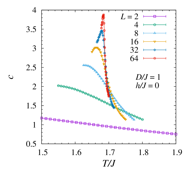
Figure 1: (Color online) Temperature dependence of the specific heat $c$ of the chiral helimagnetic model in three dimensions without magnetic fields.

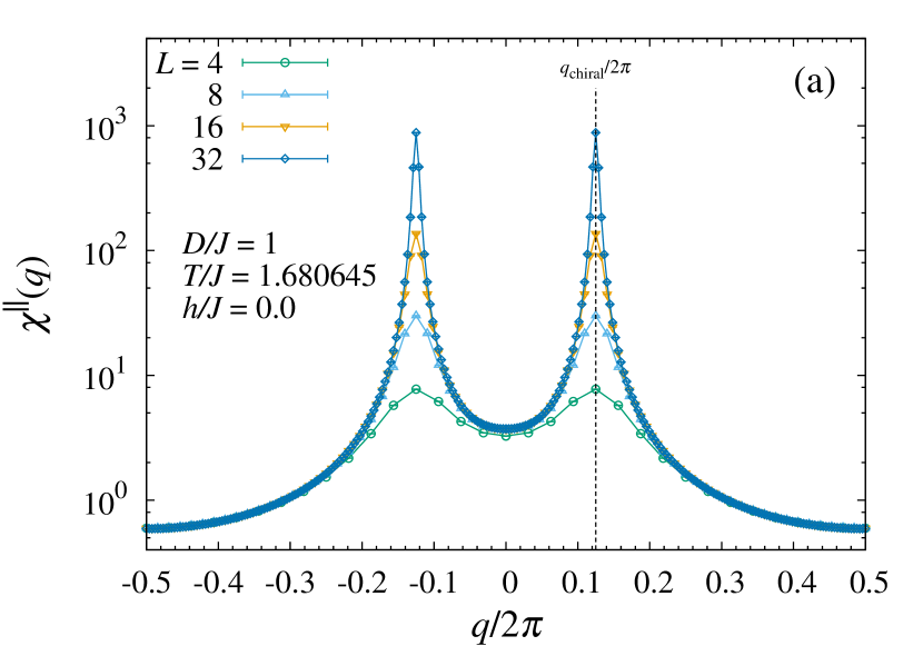
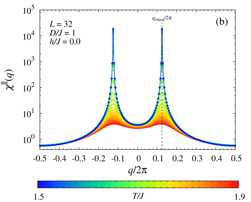
Figure 2: (Color online) Wave-number dependence of $\chi^{\parallel}\left(q\right)$ of the three-dimensional chiral helimagnetic model without magnetic fields (a) for various system sizes at $T/J=1.680645$, which is close to the critical temperature, and (b) with $L=32$ at various temperatures above and below the critical temperature.

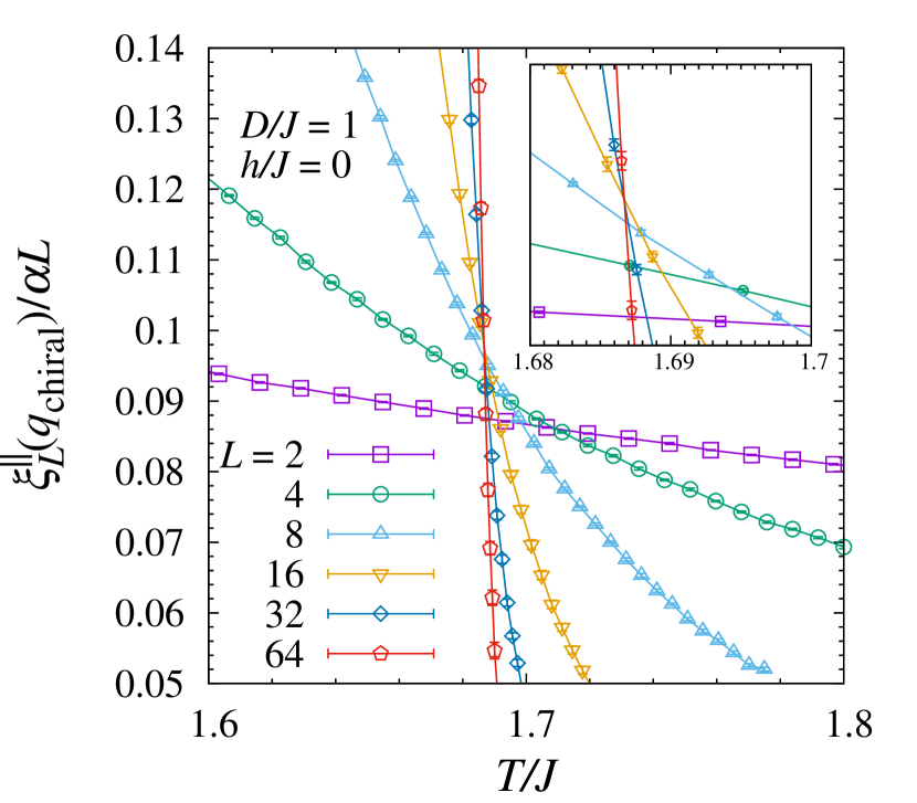
Figure 3: (Color online) Temperature dependence of the finite-size correlation length $\xi_{L}(q_{\mathrm{chiral}})$ divided by $\alpha L$ of the three-dimensional chiral helimagnetic model without magnetic fields. The inset presents an enlarged view around the critical temperature.

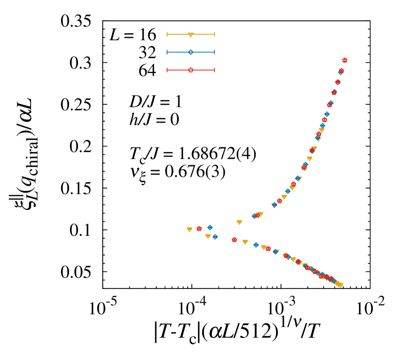
Figure 4: (Color online) A finite-size scaling plot of the finite-size correlation length $\xi^{\parallel}_{L}\left(q_{\mathrm{chiral}}\right)$ divided by $\alpha L$ of the three-dimensional chiral helimagnetic model without magnetic fields. The smallest system size of this FSS plot is $L_{\mathrm{min}}=16$. The critical temperature $T_{\mathrm{c}}$ and the critical exponent $\nu$ are estimated as $T_{\mathrm{c}}/J=1.68672(4)$ and $\nu=0.676(3)$, respectively.

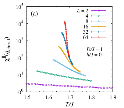
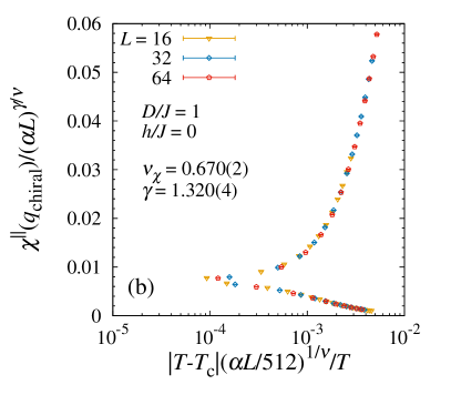
Figure 5: (Color online) (a): Temperature dependence of the wave-vector-dependent magnetic susceptibility $\chi^{\parallel}\left(q_{\mathrm{chiral}}\right)$ of the chiral helimagnetic model in three dimensions without magnetic fields. (b): A finite-size scaling plot of $\chi^{\parallel}\left(q_{\mathrm{chiral}}\right)$ of the chiral helimagnetic model in three dimensions without magnetic fields. The value of the critical temperature $T_{\mathrm{c}}$ estimated by the finite-size scaling analysis of the finite-size correlation length ratio $\xi^{\parallel}_{L}\left(q_{\mathrm{chiral}}\right)/\alpha L$ is used.

IV Result

In this section, we present results of our Monte Carlo simulations of the system with and without the magnetic field. The linear size of the system in the simulations ranges from $L=2$ (the total number of spins $N=2\times 16\times 2$) to $L=64$ ($N=64\times 512\times 64$). The total number of Monte Carlo steps (MCS) in our simulations is $5\times 10^{4}$ – $5\times 10^{5}$ depending on the system size, where one MCS is defined as $N$ lifting events with $5$ over-relaxation sweeps per spin. One heat-bath update per spin is performed for every $10$ MCS. We checked the equilibration by confirming that the average values of physical quantities measured during an interval coincide with those measured during another interval twice longer within statistical uncertainty. Error bars are evaluated by results of multiple independent simulations.

IV.1 Universality class of the system without magnetic fields

First, we present the specific heat $c$ of the system for various system sizes in Fig. 1. One can see in the figure that the specific heat shows a sharp peak at about $T/J\simeq 1.68$, and thus, a phase transition is expected to occur at around this temperature. Around and below this temperature, the wave-vector-dependent susceptibility $\chi^{\parallel}\left(q\right)$ has two peaks at $q=\pm q_{\mathrm{chiral}}$, see Fig. 2. This fact is insensitive to the system size in our simulations. Therefore, the wave vector $\boldsymbol{q}_{\mathrm{chiral}}$ also characterizes the ordering structure of the system at finite temperature and $\boldsymbol{m}\left(\boldsymbol{q}_{\mathrm{chiral}}\right)$ can be considered as an order parameter of the system.

We show the wave-vector-dependent finite-size correlation length $\xi^{\parallel}_{L}\left(q_{\mathrm{chiral}}\right)$ divided by $\alpha L$ in Fig. 3. One can see in the figure that each pair of curves for $\xi_{L}^{\parallel}\left(q_{\mathrm{chiral}}\right)/\alpha L$ and $\xi_{2L}^{\parallel}\left(q_{\mathrm{chiral}}\right)/2\alpha L$ intersects at a temperature and that the intersection converges to a certain temperature point for larger sizes while it slightly shifts for smaller sizes. This implies that the correlation length with the wave vector $\boldsymbol{q}_{\mathrm{chiral}}$ diverges at a finite temperature in the thermodynamic limit. Here, we assume that $\xi_{L}^{\parallel}\left(q_{\mathrm{chiral}}\right)/\alpha L$ follows a finite-size scaling (FSS) form

$$\frac{\xi_{L}^{\parallel}\left(q_{\mathrm{chiral}}\right)}{\alpha L}=F\left[\left(T-T_{\mathrm{c}}\right)\left(\alpha L\right)^{1/\nu}\right],$$ (21)

where $F$ is a scaling function and $\nu$ is the critical exponent of the correlation length. By using a recently proposed method based on Bayesian inference Harada (2011, 2015), FSS analyses are performed for four sets of the data consisting of three successive system sizes $L_{\mathrm{min}}$, $2L_{\mathrm{min}}$ and $4L_{\mathrm{min}}$. As shown in Fig. 4, the FSS plot for the data set with $L_{\mathrm{min}}=16$ works well, yielding that the critical temperature $T_{\mathrm{c}}$ and the critical exponent $\nu$ are estimated as $T_{\mathrm{c}}/J=1.68672(4)$ and $\nu=0.676(3)$, respectively.

Using the value of the critical temperature estimated by FSS of the finite-size correlation length ratio $\xi_{L}^{\parallel}\left(q_{\mathrm{chiral}}\right)/\alpha L$, we also perform FSS analyses of the wave-vector-dependent susceptibility $\chi^{\parallel}\left(q_{\mathrm{chiral}}\right)$ for the same data sets. The susceptibility is assumed to follow a scaling form

$$\chi^{\parallel}\left(q_{\mathrm{chiral}}\right)=\left(\alpha L\right)^{\gamma/\nu}G\left[\left(T-T_{\mathrm{c}}\right)\left(\alpha L\right)^{1/\nu}\right],$$ (22)

where $G$ is a scaling function and $\gamma$ is the critical exponent of the susceptibility. One can see in Fig. 5 temperature dependence of the susceptibility $\chi^{\parallel}\left(q_{\mathrm{chiral}}\right)$ and the resultant FSS plot. The exponents are estimated as $\nu=0.670(2)$ and $\gamma=1.320(4)$, respectively. The estimated values of the critical temperature and exponents are shown in Table 1. As seen in the table, the values of the critical exponents approach those of the three-dimensional ferromagnetic XY model Campostrini et al. (2001) as $L_{\mathrm{min}}$ increases. We conclude that the system without magnetic fields undergoes a phase transition from a paramagnetic phase to a chiral helimagnetic phase as temperature decreases with critical exponents of the three-dimensional XY model, as predicted in Ref. Liu, 1973; Klein and Aharony, 1991; Calvo, 1981.

$L_{\mathrm{min}}$	$T_{\mathrm{c}}/J$	$\nu_{\xi}$	$\nu_{\chi}$	$\gamma$
2	1.688(1)	0.72(2)	0.711(5)	1.45(1)
4	1.6871(2)	0.696(5)	0.682(2)	1.314(4)
8	1.68683(5)	0.681(4)	0.671(1)	1.303(3)
16	1.68672(4)	0.676(3)	0.670(2)	1.320(4)

Table 1: The estimated values of the critical temperature and the critical exponents of the correlation length and the susceptibility by finite-size scaling analyses. The values of the critical temperature $T_{\mathrm{c}}$ and the exponent of the correlation length denoted as $\nu_{\xi}$ are estimated using the data of the finite-size correlation length $\xi^{\parallel}_{L}\left(q_{\mathrm{chiral}}\right)/\alpha L$. Using the estimated value of $T_{\mathrm{c}}$, the value of critical exponents of the susceptibility $\gamma$ and that of the correlation length denoted as $\nu_{\chi}$ are estimated by FSS analyses of the susceptibility $\chi^{\parallel}\left(q_{\mathrm{chiral}}\right)$.

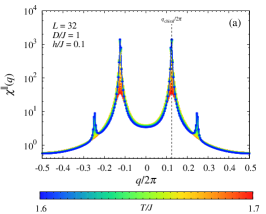
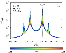
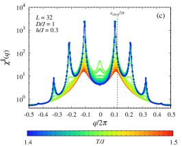
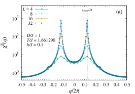
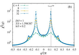
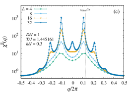
Figure 6: (Color online) Wave-number dependence of $\chi^{\parallel}\left(\boldsymbol{q}\right)$ of the chiral helimagnetic model in three dimensions for various temperatures with $L=32$. The values of the magnetic fields perpendicular to the DM vector are (a) $h/J=0.1$, (b) $h/J=0.2$, and (c) $h/J=0.3$. The vertical line represents $q_{\mathrm{chiral}}/2\pi$.

Figure 7: (Color online) Wave-number dependence of $\chi^{\parallel}\left(\boldsymbol{q}\right)$ of the chiral helimagnetic model in three dimensions for various system sizes near the estimated transition temperature depending on the magnetic field. The values of the magnetic fields perpendicular to the DM vector are (a) $h/J=0.1$, (b) $h/J=0.2$, and (c) $h/J=0.3$.

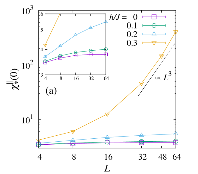
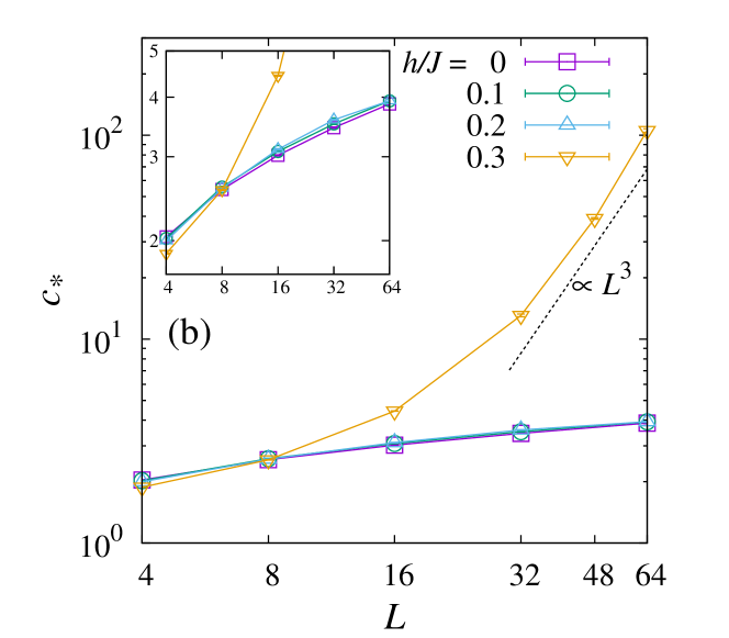
Figure 8: (Color online) System-size dependence of the peak value of the susceptibility $\chi^{\parallel}_{*}\left(0\right)$ (a) and the specific heat $c_{*}$ (b) of the chiral helimagnetic model in three dimensions with a magnetic field perpendicular to the DM vector $h/J=0$, $0.1$, $0.2$, and $0.3$. The black dotted lines are proportional to $L^{3}$. The insets show enlarged views.

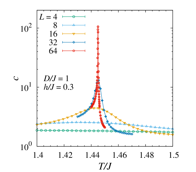
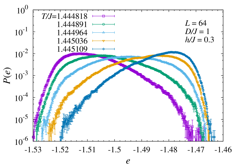
Figure 9: (Color online) Temperature dependence of specific heat $c$ of the chiral helimagnetic model in three dimensions with a magnetic field perpendicular to the DM vector $h/J=0.3$.

Figure 10: (Color online) The energy-density distribution function $P\left(e\right)$ of the chiral helimagnetic model in three dimensions with a magnetic field perpendicular to the DM vector $h/J=0.3$. The system size $L=64$ is the largest size in our simulations and the temperatures are close to the transition temperature.

IV.2 Phase transition under a magnetic field perpendicular to the DM vector

In this subsection, we focus on the effect of a magnetic field perpendicular to the DM vector. The wave-number dependence of the susceptibility $\chi^{\parallel}\left(q\right)$ at $h/J=0.1$, $0.2$, and $0.3$ for various temperatures and various sizes is shown in Fig. 7 and Fig. 7, respectively. In contrast to the case without the magnetic field shown in Fig. 2, $\chi^{\parallel}\left(q\right)$ has several peaks at $\pm q_{0}$ and integral multiples of $q_{0}$ in the presence of the magnetic field in the low temperature region with $q_{0}$ being the positive wave number which gives the largest value of the susceptibility. The value of $q_{0}$ for finite magnetic fields is significantly smaller than that of $q_{\mathrm{chiral}}$, although the difference is tiny for small fields as shown in Fig. 7 and Fig. 7. Furthermore, not only the largest peaks but also other small peaks are enhanced with increasing the system size, as seen in Fig. 7. These indicate that a periodic order, e.g., chiral soliton lattice (CSL) which cannot be characterized by a single wave vector emerges at low temperatures in the thermodynamic limit. The distance between two chiral solitons in the low temperature region is characterized by the value of the wave number $q_{0}$ as $\sim 2\pi/\left|q_{0}\right|$. In Fig. 7(c), for instance, one can see that $\left|q_{0}\right|/2\pi\sim 0.1$ at a sufficiently low temperature for $h/J=0.3$, and hence, the distance between two chiral solitons along the DM vector is about $10$ lattice spacings. Other wave numbers of the peak in $\chi^{\parallel}\left(q\right)$ in the low temperature region are considered to characterize shorter length scales within one chiral soliton.

One may consider naively the order parameter of the CSL order to be $\boldsymbol{m}\left(\boldsymbol{q}_{0}\right)$. The value of $q_{0}$ weakly depends on temperature and also the values of the wave numbers of the peaks in finite systems with the magnetic field slightly deviate from those in the thermodynamic limit. The latter is due to the fact that the wave number in finite-size lattices can take only discrete values. As discussed above, the existence of the CSL phase characterized by the multiple wave vectors is strongly suggested at low temperatures. It is, however, difficult to identify the precise value of $q_{0}$ in numerical simulations and the order parameter in the CSL phase.

While the CSL emerges in the presence of the magnetic field, qualitatively different behavior is observed in thermodynamic quantities at a relatively large magnetic field, particularly at $h/J=0.3$ in our study. One of the striking features is the existence of the sharp peak of $\chi^{\parallel}\left(0\right)$ at a certain temperature which is not the intrinsic susceptibility conjugated with the CSL order and also the chiral helimagnetic order parameter. At the temperature, the specific heat has a diverging peak simultaneously. We show in Fig. 8 the system-size dependence of the peak values of the magnetic susceptibility $\chi^{\parallel}_{*}\left(0\right)$ and the specific heat $c_{*}$. For $h/J=0.1$ and $0.2$, the peak values of $\chi^{\parallel}_{*}\left(0\right)$ and $c_{*}$ do not seem to diverge even in the thermodynamic limit. This is compatible with the result of $h/J=0$, where the system belongs to the universality class of the three-dimensional XY model and hence the critical exponent $\alpha$ is negative. Without the magnetic field, the specific heat $c$ does not diverge, but shows a cusp singularity at the critical temperature in the thermodynamic limit as the three-dimensional XY model. When a cusp singularity exists in the specific heat, its peak value $c_{*}$ scales as Peczak et al. (1991); Holm and Janke (1993)

$$c_{*}\simeq c_{*}^{\infty}-sL^{\alpha/\nu},$$ (23)

where $c_{*}^{\infty}$ is the peak value of the specific heat in the thermodynamic limit and $s$ is a constant. We can see in the inset of Fig. 8(b) that the peak values $c_{*}$ of the system with $h/J=0$, $0.1$ and $0.2$ have very similar system size dependence. This fact suggests that the system under the magnetic fields also belongs to the universality class of the three-dimensional ferromagnetic XY model.

On the other hand, for $h/J=0.3$, the peak values $\chi^{\parallel}_{*}\left(0\right)$ and $c_{*}$ show very strong tendencies to diverge in the thermodynamic limit. In particular, $\chi^{\parallel}_{*}\left(0\right)$ and $c_{*}$ at $h/J=0.3$ seem to diverge as a power law with $L^{3}$ or even faster than a power low in larger system sizes. These indicate the existence of a critical point $\left(T_{\mathrm{d}},h_{\mathrm{d}}\right)$ where $0.2<h_{\mathrm{d}}/J<0.3$ on the phase boundary between the paramagnetic phase and the CSL phase in the magnetic phase diagram of the system. In other words, the system is expected to have finite values of the specific heat $c$ and the susceptibility $\chi^{\parallel}\left(0\right)$ at the transition temperature for $h<h_{\mathrm{d}}$, and presumably belongs to the same universality class of the system without the magnetic field, while the system undergoes a phase transition at a finite temperature with the diverging specific heat $c$ and diverging magnetic susceptibility $\chi^{\parallel}\left(0\right)$ for $h>h_{\mathrm{d}}$.

A possible explanation of the strong divergence of the specific heat found at $h/J=0.3$ might be an occurrence of the first-order phase transition. Then, the specific heat has a delta-function type divergence at the transition temperature and the peak value of the specific heat is expected to diverge as $L^{d}$ where $d=3$ is the spatial dimension Fisher and Berker (1982). Also the energy-density distribution has two peaks at the transition temperature. In Fig. 10, we present temperature dependence of the specific heat $c$ of the system with $h/J=0.3$. One can see in the phase diagram that the specific heat $c$ shows a very sharp peak at about $T/J\simeq 1.445$, and the width of the peak becomes narrower as the system size increases. This is consistent with the occurrence of the first-order transition and the size dependence of $c_{*}$ shown in Fig. 8(b) is marginally compatible with $L^{3}$. However, as seen in Fig. 10, the energy-density distribution function $P\left(e\right)$ does not have a double-peak structure near the transition temperature. No clear evidence of the first-order transition is found in our numerical results. We could not completely rule out the possibility of a weak first-order transition with a finite correlation length at the transition temperature larger than the largest system size in our simulations. Therefore, we tentatively conclude that this phase transition found at $h/J=0.3$ is a continuous one. Our results suggest that the expected universality class has a ratio of the critical exponents of the specific heat and the correlation length $\alpha/\nu>3$, assuming that $c_{*}$ of the system diverges faster than $L^{3}$ also in larger systems. Unfortunately, we could not determine the critical exponents of the transition and the precise location of the critical point $\left(T_{\mathrm{d}},h_{\mathrm{d}}\right)$, which requires larger scale simulations of the system.

V Discussion and Summary

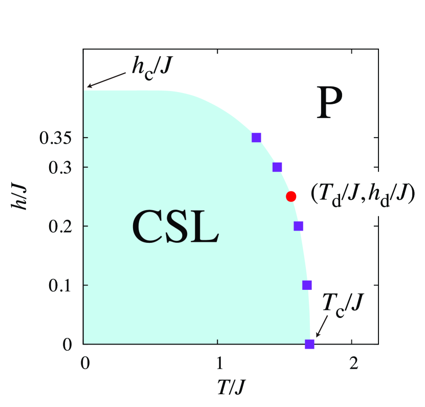
Figure 11: (Color online) A possible magnetic phase diagram of the chiral helimagnetic model in three dimensions. In the phase diagram, “CSL” and “P” denote the chiral soliton lattice phase and paramagnetic phase, respectively. The filled squares are estimated transition temperature in this work and the circle represents an expected critical point whose precise location is not determined.

A possible phase diagram of the system is presented in Fig. 11, where we denote the paramagnetic phase and the CSL phase as “P” and “CSL”, respectively. The filled square at $h/J=0$ is estimated by the FSS analysis in Sec. IV.1, and other squares are estimated by the peak temperature of $\chi^{\parallel}\left(0\right)$ at $h/J=0.1$, $0.2$ and $0.3$ for $L=64$ and at $h/J=0.35$ for $L=16$. The circle represents an expected location of the critical point $\left(T_{\mathrm{d}}/J,h_{\mathrm{d}}/J\right)$.

One can see in the phase diagram that the phase boundary $h_{\partial\mathrm{CSL}}\left(T\right)$ between the paramagnetic phase and the CSL phase has a finite slope, which is compatible with the experimental phase diagram of a chiral helimagnet Togawa et al. (2013). Imposing differentiability on the free-energy density of the infinite system at a point $\left(T_{0},h_{\partial\mathrm{CSL}}\left(T_{0}\right)\right)$ where a second-order phase transition occurs, the finite tangent of the phase boundary yields the relation

$$\Delta\chi\Delta c-T\left(\Delta\omega\right)^{2}=0,$$ (24)

where $\omega$ and $\chi$ are the temperature derivative and the magnetic-field derivative of the magnetization parallel to the field, and $\Delta X=X_{\rm CLS}-X_{\rm P}$ for any $X\in\{c,\chi,\omega\}$ at $\left(T_{0},h_{\partial\mathrm{CSL}}\left(T_{0}\right)\right)$, respectively. If the system under the magnetic field with $0<h<h_{\mathrm{d}}$ belongs to the universality class of the three-dimensional ferromagnetic XY model as discussed above, the specific heat is continuous on the phase boundary. In this system for a fixed $h<h_{\mathrm{d}}$, the uniform susceptibility has a finite value. Therefore, Eq. (24) requires $\Delta\omega=0$, meaning that the magnetization parallel to the magnetic field is smooth at the transition temperature.

For $h>h_{\mathrm{d}}$, however, the strong divergence is found in the specific heat. The difference $\Delta c$ is infinitely large unless the critical amplitude ratio is accidentally 1 with the same critical exponent above and below the critical temperature which may unlikely occur in finite dimensions. Then, the relation of Eq. (24) allows typically two cases: (i) $\Delta\chi=0$ and $\Delta\omega$ is finite and (ii) $\Delta\chi=\infty$ and $\Delta\omega=\infty$. Our result of the divergence of $\chi^{\parallel}\left(0\right)$ indicates the latter case. Precisely speaking, $\chi$ is not identical with $\chi^{\parallel}\left(0\right)$ but $\Delta\chi$ likely diverges when $\chi^{\parallel}\left(0\right)=\infty$. This implies that the exponent of the divergence of $\chi^{\parallel}\left(0\right)$ coincides with that of the specific heat. Furthermore, the temperature dependence of the magnetization is also described by the same singularity at least either above or below the critical temperature. Thus, the critical singularity of the specific heat appears in other observables unrelated to the critical nature through the relation of Eq. (24), while in a conventional system where $\chi$ is an order-parameter susceptibility, the relation yields the scaling relation $\alpha+2\beta+\gamma=2$ among the critical indices.

We should note here that Dzyaloshinskii predicts by analyzing the one-dimensional continuum model of the chiral helimagnet in the presence of the magnetic field that a continuous phase transition occurs at a finite temperature Dzyaloshinskii (1965). It is also shown that the specific heat diverges from below the transition temperature with a logarithmic correction as

$$c\propto\frac{1}{\left(T_{*}-T\right)\log^{2}\left(T_{*}-T\right)},$$ (25)

where $T_{*}$ is the transition temperature, while no divergence of $c$ displays from above $T_{*}$. In this case, $\Delta c$ is infinity at $T_{*}$ and the critical exponent of the specific heat $\alpha^{\prime}=1$ below $T_{*}$ and $\alpha=0$ above $T_{*}$. Although no definite conclusion can be drawn on the validity of this peculiar prediction, our numerical data of the specific heat is not inconsistent with the asymmetric behavior between above and below the critical temperature. One of the main difficulties in determining the critical indices is due to the logarithmic-correction term, which makes the critical region narrow. Assuming the hyperscaling relation $d\nu=2-\alpha$ and $\alpha=1$, the critical exponent of the correlation length is $\nu=1/3$, and hence, the peak value of the specific heat is expected to diverge as $\sim L^{\alpha/\nu}=L^{3}$. It also coincides with that in the system with the first-order transition. As discussed in IV.2, the power-law divergence of $c_{*}$ with $L^{3}$ is marginally consistent with our numerical result. Further investigations are required to clarify the nature of the phase transition of the system with $h>h_{\mathrm{d}}$ and examine the validity of Dzyaloshinskii’s theory Dzyaloshinskii (1965).

In summary, we have numerically studied the classical Heisenberg spin model of a chiral helimagnet in three dimensions by equilibrium Monte Carlo simulations using the event-chain algorithm. We have particularly focused on its finite-temperature phase transitions with and without a magnetic field perpendicular to the axis of the helical structure. Without the magnetic field, it is shown by the FSS analysis that the system undergoes a continuous phase transition with critical exponents of the three-dimensional ferromagnetic XY model as predicted by some theoretical studies. It is found that the nature of phase transitions changes in the presence of the magnetic field, although we speculate that the phase transition is continuous irrespectively with the value of the magnetic field $h$. While the specific heat $c$ and the magnetic susceptibility $\chi^{\parallel}\left(0\right)$ have finite values at the transition temperature for $h/J=0.1$ and $0.2$, they diverge at the transition temperature for $h/J=0.3$. Consequently, it is suggested that the critical point $\left(T_{\mathrm{d}},h_{\mathrm{d}}\right)$ exists in the region where $0.2<h_{\mathrm{d}}/J<0.3$ in the phase diagram of the system. The critical exponents of the phase transitions at and above $h_{\mathrm{d}}$ remain unclear, and thus it would be interesting to reveal the universality class of the phase transition in high fields by determining the critical exponents. A promising way for studying the phase structure might be the method of renormalization group. Our results suggest that the phase transition, distinct from the transition at the low fields, can be detected as a strong singularity in the specific heat, uniform susceptibility and also magnetization curve, which are measurable in experiments. However, the amplitude of the DM interaction studied in this paper is rather large from viewpoint of experiments. Thus, the dependence of the critical point is to be clarified in comparison with the experiments.