Constant slope maps on the extended real line

Abstract.

For a transitive countably piecewise monotone Markov interval map we consider the question whether there exists a conjugate map of constant slope. The answer varies depending on whether the map is continuous or only piecewise continuous, whether it is mixing or not, what slope we consider, and whether the conjugate map is defined on a bounded interval, half-line or the whole real line (with the infinities included).

1. Introduction

Among piecewise monotone interval maps, the simplest to understand are the piecewise linear maps with the same absolute value of slope on every piece; such maps are said to have constant slope (and we will usually say “slope” in the meaning “absolute value of slope”). These maps offer the dynamicist many advantages. For example, if we wish to compute the topological entropy, we just take the larger of zero and the logarithm of the slope. If we wish to study the symbolic dynamics and the slope is larger than one, then no two points can share the same itinerary; this already rules out wandering intervals.

There are two classic results by which constant slope maps provide a good model for understanding more general piecewise monotone maps. Nearly fifty years ago, Parry proved that every topologically transitive, piecewise monotone (and even piecewise continuous) interval map is conjugate to a map of constant slope [8]. Then, in the 1980’s, Milnor and Thurston showed how to modify Parry’s theorem to remove the hypothesis of topological transitivity [5]. As long as a piecewise monotone map has positive topological entropy $\log\lambda$, there exists a semiconjugacy to a map of constant slope $\lambda$. The semiconjugating map is nondecreasing, preserving the order of points in the interval, but perhaps collapsing some subintervals down to single points.

It is natural to ask how well the theory extends to countably piecewise monotone maps, when we no longer require the set of turning points to be finite, but still require it to have a countable closure. The theory has to be modified in several ways. In contrast to Parry’s result, it is possible to construct transitive examples which are not conjugate to any interval map of constant slope. Such examples are contained in the authors’ prior publication [7]. However, those particular examples are conjugate to constant slope maps on the extended real line $[-\infty,\infty]$, which we may choose to regard as an interval of infinite length. In response, Bobok and Bruin posed the following problem: Under what conditions does a countably piecewise monotone interval map admit a conjugacy to a map of constant slope on the extended real line?

The present paper answers this problem, focusing on the Markov case. Section 2 gives the necessary definitions, then closes with a theorem due to Bobok [2], that there exists a nondecreasing semiconjugacy to a map of constant slope $\lambda>1$ on the finite length interval $[0,1]$ if and only if the relevant transition matrix admits a nonnegative eigenvector with eigenvalue $\lambda$ and summable entries.

We investigate whether eliminating the summability requirement on the eigenvector might allow for the construction of constant slope models on the extended real line. We find two new obstructions, not present in previous works. We present one example which is topologically transitive but not mixing (Section 12), and one example which is mixing but only piecewise continuous (Section 11), and we show for both of these examples that although the transition matrix admits a nonnegative eigenvector with some eigenvalue $\lambda$, nevertheless there is no conjugacy to any map of constant slope $\lambda$. These are the only two obstructions; under the assumptions of continuity and topological mixing, we state in Section 3 our main theorem, Theorem 3.1, that a countably piecewise monotone and Markov map which is continuous and mixing admits a conjugacy to a map of constant slope $\lambda$ on some non-empty, compact (sub)interval of the extended real line $[-\infty,\infty]$ if and only if the associated Markov transition matrix admits a nonnegative eigenvector of eigenvalue $\lambda$. Sections 4 through 7 are dedicated to the proof of Theorem 3.1.

Sections 8 through 10 apply Theorem 3.1 to three explicit examples of continuous countably piecewise monotone Markov maps. The first admits conjugate maps of constant slope on the unit interval. The second admits conjugate maps of constant slope on the extended real line and the extended half line. The third does not admit any conjugate map of constant slope. These sections illustrate a variety of novel techniques for calculating the nonnegative eigenvectors of a countable 0-1 matrix and for calculating the topological entropy of a countably piecewise monotone map.

2. Definitions and Background

The extended real line $[-\infty,\infty]$ is the ordered set $\mathbb{R}\cup\{\infty,-\infty\}$ equipped with the order topology; this topological space is a two-point compactification of the real line and is homeomorphic to the closed unit interval $[0,1]$.

There is an exceedingly simple example which illustrates how the extended real line behaves differently than the unit interval with respect to constant slope maps. Consider the map $f:[0,1]\to[0,1]$ given by $f(x)=x^{2}$. A conjugate map on the unit interval must be monotone with fixed points at $0$ and $1$, and the only constant slope map with those properties is the identity map. On the other hand, the map $g:[-\infty,\infty]\to[-\infty,\infty]$ given by $g(x)=x-1$ has constant slope $1$ and is conjugate to $f$ by the homeomorphism $h:[0,1]\to[-\infty,\infty]$, $h(x)=-\log_{2}(-\log_{2}(x))$. Thus, we achieve constant slope by taking advantage of the infinite length of the extended real line and pushing our fixed points out to $\pm\infty$, see Figure 1.

.

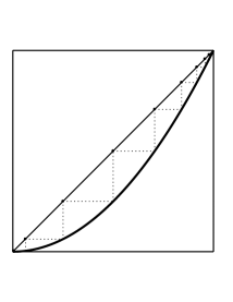
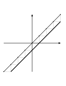
Figure 1. A conjugacy which moves the fixed points to $\pm\infty$.

Suppose $f$ is a continuous self-map of some interval $[a,b]$, $-\infty\leq a<b\leq\infty$, and suppose there exists a closed, countable set $P\subset[a,b]$, $a,b\in P$, such that $f(P)\subset P$ and $f$ is monotone on each component of $[a,b]\setminus P$. Such a map is said to be countably piecewise monotone and Markov with respect to the partition set $P$; the components of $[a,b]\setminus P$ are called $P$-basic intervals, and the set of all $P$-basic intervals is denoted $\mathcal{B}(P)$. If additionally the restriction of $f$ to each $P$-basic interval is affine with slope of absolute value $\lambda$, then we say that $f$ has constant slope $\lambda$. This is a geometric, rather than a topological property, and it is the reason we must distinguish finite from infinite length intervals. The class of all continuous countably piecewise monotone and Markov maps is denoted $\mathcal{CPMM}$. The subclass of those maps which act on the closed unit interval $[0,1]$ is denoted $\mathcal{CPMM}_{[0,1]}$.

Let us draw the reader’s attention to three properties of the class $\mathcal{CPMM}$. First, the underlying interval $[a,b]$ depends on the map $f$ and is permitted to be infinite in length. Second, the map $f$ is required to be globally (rather than piecewise) continuous; this is essential for our use of the intermediate value theorem. And third, the set $P$ is required to be forward-invariant. This is the Markov condition; it means that if $I$, $J$ are $P$-basic intervals and $f(I)\cap J\neq\emptyset$, then $f(I)\supseteq J$.

If $f$ is countably piecewise monotone and Markov with respect to $P$, then we define the binary transition matrix $T=T(f,P)$ with rows and columns indexed by $\mathcal{B}(P)$ and entries

(1) $$T(I,J)=\begin{cases}1,&\textnormal{ if }f(I)\supseteq J\\ 0,&\textnormal{ otherwise.}\end{cases}$$

This transition matrix represents a linear operator on the linear space $\mathbb{R}^{\mathcal{B}(P)}$ without any reference to topology. In particular, in Theorem 2.1 below, $T$ is not required to represent a bounded operator on $\ell^{1}(\mathbb{R}^{\mathcal{B}(P)})$, nor even to preserve the subspace $\ell^{1}(\mathbb{R}^{\mathcal{B}(P)})\subset\mathbb{R}^{\mathcal{B}(P)}$.

We wish also to study maps which are only piecewise continuous. To that end, we define the class $\mathcal{CPMM}^{pc}$ which contains any self-map $f$ of any closed, nonempty interval $[a,b]\subset[-\infty,\infty]$, such that $f$ has the following properties with respect to some closed, countable set $P\subset[a,b]$, $a,b\in P$, namely, that $f(P)\subset P$, that the restriction $f|_{I}$ is strictly monotone and continuous for each $P$-basic interval $I\in\mathcal{B}(P)$, and that for each pair $I,J\in\mathcal{B}(P)$, either $f(I)\cap J=\emptyset$ or else $f(I)\supseteq J$. Note that this definition places no continuity requirements on the map $f$ at the points of $P$. Studies on finitely piecewise continuous maps often require one-sided continuity at the endpoints of the basic intervals (allowing the map to take 2 values at a single point), but our countable set $P$ may have accumulation points which are not the endpoint of any $P$-basic interval, so such an approach makes no sense here. We define also the subclass $\mathcal{CPMM}^{pc}_{[0,1]}$ for those maps which act on the closed unit interval $[0,1]$, and we define the binary transition matrix $T=T(f,P)$ by the same formula (1) as before.

We will also have cause to consider the properties of topological transitivity and topological mixing. We use the standard definitions, that a map $f$ is topologically transitive (respectively, topologically mixing) provided that for every pair of nonempty open sets $U,V$ there exists $n_{0}\in\mathbb{N}$ such that $f^{n_{0}}(U)\cap V\neq\emptyset$ (respectively, for all $n\geq n_{0}$, $f^{n}(U)\cap V\neq\emptyset$).

If we ignore the extended real line $[-\infty,\infty]$ and allow only for maps on the unit interval $[0,1]$, then there is already an established necessary and sufficient condition to determine when a map is semiconjugate to a map of constant slope.

Theorem 2.1.

(Bobok, [2]) Let $f\in\mathcal{CPMM}^{pc}_{[0,1]}$ be a map with partition set $P$ and transition matrix $T$, and fix $\lambda>1$. Then $f$ is semiconjugate via a continuous nondecreasing map $\psi$ to some map $g\in\mathcal{CPMM}^{pc}_{[0,1]}$ of constant slope $\lambda$ if and only if $T$ has a nonnegative eigenvector $v=\left(v_{I}\right)\in\ell^{1}(\mathbb{R}^{\mathcal{B}(P)})$ with eigenvalue $\lambda$.

Remark 2.2.

The statement of Theorem 2.1 in [2] is for the class $\mathcal{CPMM}_{[0,1]}$ of globally continuous maps, but the proof applies equally well in the piecewise continuous setting.

We draw the reader’s attention to the requirement $v\in\ell^{1}(\mathbb{R}^{\mathcal{B}(P)})$ that the eigenvector should be summable. If we read the proof in [2], the reason for this is clear. If we are given the semiconjugacy $\psi$ to the constant slope map, then we construct the eigenvector $v$ by setting $v_{I}=|\psi(I)|$ for each $P$-basic interval $I$, where $|\cdot|$ denotes the length of an interval, and therefore the sum of the entries $v_{I}$ is just the length of the unit interval $[0,1]$. Conversely, if we are given an eigenvector $v$, then we rescale it so that the sum of entries is $1$ and then construct the semiconjugacy in such a way that $|\psi(I)|=v_{I}$ for all $I$, obtaining a map $g$ of an interval of length $1$.

3. Statement of Main Results

We return now to the question, when does a map $f\in\mathcal{CPMM}$ admit a nondecreasing semiconjugacy $\psi$ to a map $g$ of constant slope on some compact subinterval of $[-\infty,\infty]$, whether finite or infinite in length? It is clear that $g$ must belong to the class $\mathcal{CPMM}$, because $g$ will necessarily be piecewise monotone and Markov with respect to $\psi(P)$ – see [1, Lemma 4.6.1]. Here are the statements of our main results:

Theorem 3.1.

Let $f\in\mathcal{CPMM}$ be a map with partition set $P$ and transition matrix $T$, and fix $\lambda>1$. Assume that $f$ is topologically mixing. Then $f$ is conjugate via a homeomorphism $\psi$ to some map $g\in\mathcal{CPMM}$ of constant slope $\lambda$ if and only if

(2) $$T\textnormal{{ has a nonnegative eigenvector }}v=(v_{I})\in\mathbb{R}^{\mathcal{B}(P)}\textnormal{{ with eigenvalue }}\lambda.$$

Theorem 3.2.

In the piecewise continuous case (replacing $\mathcal{CPMM}$ by $\mathcal{CPMM}^{pc}$), condition (2) is necessary but not sufficient.

Theorem 3.3.

If we replace the hypothesis of topological mixing with the weaker condition of topological transitivity, then condition (2) is necessary but not sufficient.

Remark 3.4.

Since the map $f$ in Theorem 3.1 defines a topological dynamical system without regard to geometry, there is no loss of generality if we assume that $f\in\mathcal{CPMM}_{[0,1]}$. We will make this assumption from now on.

We will start by showing the necessity of condition (2). The same proof applies in all cases (continuous or piecewise continuous, mixing or transitive). Showing the sufficiency of condition (2) in Theorem 3.1 requires much more work. We give an explicit construction of the conjugating map $\psi$ in several stages. Our construction begins very much like the proofs of [2, Theorem 2.5] and [1, Theorem 4.6.8], but the unsummability of $v$ introduces some additional difficulties not present in these previous works. It is the strength of global continuity and topological mixing which allows us to overcome these difficulties. The insufficiency of condition (2) in Theorems 3.2 and 3.3 is proved by example in Sections 11 and 12.

4. The Proof Begins

Lemma 4.1.

(Bobok) In Theorems 3.1, 3.2, and 3.3, condition (2) is necessary.

Proof.

This proof is due to private communication with Jozef Bobok. As mentioned before, we may suppose that $f$ is defined on the finite interval $[0,1]$. Let $\psi$ be the conjugating map, $\psi\circ f=g\circ\psi$. Define $v$ by $v_{I}=|\psi(I)|$, $I\in\mathcal{B}(P)$, where $|\cdot|$ denotes the length of an interval. A priori, we may have $|\psi(I)|=\infty$; this happens if and only if $I$ contains one of the endpoints $0,1$ and $\psi$ maps this endpoint to one of $\pm\infty$. (Recall that if $0,1$ are accumulation points of $P$, then they are not endpoints of any $P$-basic interval). We want to show that all the entries of $v$ are finite. Since $g$ is monotone with slope of absolute value $\lambda$ on each $\psi(P)$-basic interval, we have

(3) $$|g(\psi(I))|=\lambda|\psi(I)|,\qquad I\in\mathcal{B}(P),$$

where if one side of the equality is infinite then so is the other. Let $\mathcal{F}$ denote the collection of all $P$-basic intervals $I$ such that $|\psi(I)|=\infty$. If $I\in\mathcal{F}$ and if $f(J)\supseteq I$, then by the conjugacy of $f$, $g$ and by equation (3), it follows that $J\in\mathcal{F}$. Now invoke topological transitivity and the Markov condition, and it follows that either $\mathcal{F}=\emptyset$ or $\mathcal{F}=\mathcal{B}(P)$.

Suppose toward contradiction that $\mathcal{F}=\mathcal{B}(P)$. Then there are neighborhoods of $\pm\infty$ on which $g$ is affine with constant slope $\lambda>1$. It follows that at least one of the points $\pm\infty$ is an attracting fixed point, or else they form an attracting two-cycle (slope larger than 1 in a neighborhood of infinity means that the images of points close to infinity are even closer to infinity). This contradicts transitivity. We may conclude that $\mathcal{F}=\emptyset$ and all entries of $v$ are finite.

We still need to show that $v$ is an eigenvector for $T$. Applying equation (3) we have

$$\lambda v_{I}=\lambda|\psi(I)|=|g(\psi(I))|=|\psi(f(I))|=\sum_{J\subset f(I)}|\psi(J)|=\sum_{J\in\mathcal{B}(P)}T_{IJ}v_{J}.$$

∎

Now we begin the long work of proving the sufficiency of condition (2) in Theorem 3.1. Let $f$, $T$, be as in the statement of the theorem, fix $\lambda>1$, and suppose $Tv=\lambda v$ for some nonzero vector $v=\left(v_{I}\right)\in\mathbb{R}^{\mathcal{B}(P)}$ with nonnegative entries. We will assume (by Remark 3.4) that $f\in\mathcal{CPMM}_{[0,1]}$. We will construct a map $\psi:[0,1]\to[-\infty,\infty]$ which is a homeomorphism onto its image in such a way that $g:=\psi\circ f\circ\psi^{-1}$ has constant slope $\lambda$. Define the sets

$$P_{n}=\bigcup_{i=0}^{n}f^{-i}(P),\,n\in\mathbb{N},\quad Q=\bigcup_{i=0}^{\infty}f^{-i}(P)$$

The set $Q$ is backward invariant by construction and forward invariant because $P$ is forward invariant. $Q$ is a dense subset of $[0,1]$ because $f$ is mixing. Choose a basepoint $p_{0}\in P$ and define $\psi$ on $Q$ by the formula

(4) $$\psi(x)=\left\{\begin{array}[]{c@{\hskip 1em}l}0,\hfil\hskip 10.00002pt&\textnormal{ if }x=p_{0}\\ \lambda^{-n}\sum\limits_{\begin{subarray}{c}J\in B(P^{n})\\ p_{0}<J<x\end{subarray}}v_{f^{n}(J)},\hfil\hskip 10.00002pt&\textnormal{ if }x\in P_{n},x>p_{0}\\ -\lambda^{-n}\sum\limits_{\begin{subarray}{c}J\in B(P^{n})\\ x<J<p_{0}\end{subarray}}v_{f^{n}(J)},\hfil\hskip 10.00002pt&\textnormal{ if }x\in P_{n},x<p_{0}\end{array}\right.$$

The choice of $p_{0}$ is somewhat arbitrary, but to simplify the proof of Lemma 4.3 (v), we insist that $0<p_{0}<1$ and that $p_{0}$ is an endpoint of some $P$-basic interval (i.e., $p_{0}$ is not a 2-sided accumulation point of $P$). This is possible because $P$ is a closed, countable subset of $[0,1]$ and hence cannot be perfect.

Remark 4.2.

In light of equation (4), we find that we are constructing a map $g$ on

• a finite interval $[a,b]$, if $\sum v_{I}<\infty$,

• an extended half-line $[a,\infty]$, if $\sum_{I<p_{0}}<\infty$ and $\sum_{I>p_{0}}=\infty$,

• an extended half-line $[-\infty,b]$, if $\sum_{l<p_{0}}=\infty$ and $\sum_{l>p_{0}}<\infty$, and

• the extended real line $[-\infty,\infty]$, if $\sum_{l<p_{0}}=\infty$ and $\sum_{l>p_{0}}=\infty$.

Lemma 4.3.

The function $\psi:Q\to[-\infty,\infty]$ has the following properties:

1. $\psi$ is well-defined; i.e. when $x\in P_{n_{1}}$ and $x\in P_{n_{2}}$, the sums agree.

2. $\psi$ is strictly monotone increasing.

3. If $x,x^{\prime}\in Q$ belong to an interval of monotonicity of $f$, then

   $$|\psi(f(x))-\psi(f(x^{\prime}))|=\lambda|\psi(x)-\psi(x^{\prime})|,$$

   where if one side of the equality is infinite, then so is the other.

4. For arbitrary $x,x^{\prime}\in Q$ we have

   $$|\psi(f(x))-\psi(f(x^{\prime}))|\leq\lambda|\psi(x)-\psi(x^{\prime})|,$$

   and we allow for the possibility that one or both sides of this inequality are infinite.

5. For $0<x<1$, $\psi(x)$ is finite.

Proof.

1. Suppose $K\in\mathcal{B}(P_{n})$. Then $f^{n}|K$ is monotone and $f^{n}(K)\in\mathcal{B}(P)$. Therefore

   $$\qquad\lambda^{-n-1}\sum\limits_{\begin{subarray}{c}J\in\mathcal{B}(P_{n+1})\\ J\subset K\end{subarray}}v_{f^{n+1}(J)}=\lambda^{-n-1}\sum\limits_{\begin{subarray}{c}J\in\mathcal{B}(P_{1})\\ J\subset f^{n}(K)\end{subarray}}v_{f(J)}=\\ =\lambda^{-n-1}\sum\limits_{J\in\mathcal{B}(P_{0})}T_{f^{n}(K)J}v_{J}=\lambda^{-n-1}\lambda v_{f^{n}(K)}=\lambda^{-n}v_{f^{n}(K)}$$

   This shows that $\psi$ is well-defined.

2. We will use the nonnegativity of the eigenvector $v$ together with the mixing hypothesis to show that the entries of $v$ must be strictly positive. Strict monotonicity of $\psi$ then follows from the definition. Since $v$ is not the zero vector, there must be some $P$-basic interval $I_{0}$ with $v_{I_{0}}\neq 0$. Let $I\in\mathcal{B}(P)$. By the mixing hypothesis, there is $n\in\mathbb{N}$ such that $(T^{n})_{II_{0}}\neq 0$. Then $v_{I}=\lambda^{-n}\sum_{J}(T^{n})_{IJ}v_{J}\geq\lambda^{-n}v_{I_{0}}>0$.

3. For $x,x^{\prime}\in Q$ there exists a common value $n\geq 1$ such that $x,x^{\prime}\in P_{n}$ (since $P_{0}\subset P_{1}\subset P_{2}\subset\cdots$). Then $f(x),f(x^{\prime})\in P_{n-1}$. By the monotonicity of $f$ between $x,x^{\prime}$, the assignment $K=f(J)$ defines a bijective correspondence

   $$\qquad\left\{J\in\mathcal{B}(P_{n}):J\mbox{ between }x,x^{\prime}\right\}\quad\longleftrightarrow\quad\left\{K\in\mathcal{B}(P_{n-1}):K\mbox{ between }f(x),f(x^{\prime})\right\}.$$

   By the definition of $\psi$ we may sum over those sets and obtain

   $$\qquad|\psi(f(x))-\psi(f(x^{\prime}))|=\sum_{K}\lambda^{-(n-1)}v_{f^{n-1}(K)}=\\ =\sum_{J}\lambda^{-(n-1)}v_{f^{n-1}(f(J))}=\lambda|\psi(x)-\psi(x^{\prime})|.$$

4. This is the inequality that survives from (iii) when we allow for folding between $x$ and $x^{\prime}$. To see it, we imitate the proof of (iii), noticing that by the intermediate value theorem the assignment $K=f(J)$ attains every interval $K$ between $f(x),f(x^{\prime})$ at least once.

5. Let $x$ be given, $0<x<1$. Assume $x<p_{0}$; the proof when $x>p_{0}$ is similar. Fix a $P$-basic interval $J_{0}$ with $p_{0}$ at one endpoint. Because $f$ is mixing, there exists $n$ such that $J_{0}\cap f^{-n}((p_{0},1))\neq\emptyset$ and $J_{0}\cap f^{-n}((0,x))\neq\emptyset$. By the intermediate value theorem there exist $x_{1},x_{2}\in J_{0}$ with $f^{n}(x_{1})=x$ and $f^{n}(x_{2})=p_{0}$. By  (iv) applied $n$ times, $|\psi(x)|\leq\lambda^{n}|\psi(x_{2})-\psi(x_{1})|$. But by (ii), $|\psi(x_{2})-\psi(x_{1})|\leq|\psi(\sup J_{0})-\psi(\inf J_{0})|$. At the two endpoints of $J_{0}$, $\psi$ takes the finite values $0$ and $v_{J_{0}}$ (or possibly $-v_{J_{0}}$).

∎

The main problem to tackle before we can extend $\psi$ to the desired homeomorphism is to show that the map we have defined so far has no jump discontinuities.

Problem 4.4.

Show that for each $x\in[0,1]$,

$$\inf\psi(Q\cap(x,1])=\sup\psi(Q\cap[0,x)),$$

except that for $x=0$ we write $\psi(0)$ in place of the supremum and for $x=1$ we write $\psi(1)$ in place of the infimum.

The resolution of this problem makes essential use of the global continuity of $f$ as well as the order structure of the interval $[0,1]$. Moreover, special treatment is required for the points $x\in Q$ – we must show the continuity of $\psi$ from each side separately. We do this by introducing a notion of “half-points.”

5. Half-Points

Construct the sets

$$\tilde{Q}=\left(Q\times\{+,-\}\right)\setminus\{(0,-),(1,+)\},\quad S=\left([0,1]\setminus Q\right)\cup\tilde{Q}$$

The way to think of this definition is that we are splitting each point $x\in Q$ into the two half-points $(x,+)$ and $(x,-)$. $S$ is the interval $[0,1]$ with each point of $Q$ replaced by half-points. We use boldface notation to represent points in $S$, whether half or whole. Thus, $\boldsymbol{x}$ may mean $x$ or $(x,+)$ or $(x,-)$, depending on the context.

Let us extend the dynamics of $f$ from $[0,1]$ to $S$. Recall that $Q$ is both forward and backward invariant. On $S\setminus\tilde{Q}=[0,1]\setminus Q$ we keep the map $f$ without change. To extend $f$ from $Q$ to $\tilde{Q}$ we define a notion of the orientation of the map at half-points. We say that $f$ is orientation-preserving (resp. orientation-reversing) at the half-point $(x,+)$ if some half-neighborhood $[x,x+\varepsilon)$ is contained in some $J\in\mathcal{B}(P)$ with $f|_{J}$ increasing (resp. decreasing). For a half-point $(x,-)$, the definition is the same, except that we look at a half-neighborhood of the form $(x-\varepsilon,x]$. It is not clear how to decide if $f$ is orientation-preserving or orientation-reversing at the accumulation points of $P$. It may happen that every half-neighborhood of $x$ contains $f(x)$ in the interior of its image, so that neither definition is appropriate. Nevertheless, we define the extended map $f$ on $\tilde{Q}$ by the following formula:

(5) $$f(x,+) =\begin{cases}(f(x),+),&\textnormal{ if }f\textnormal{ is orientation-preserving at }(x,+)\\ (f(x),-),&\textnormal{ if }f\textnormal{ is orientation-reversing at }(x,+)\\ (f(x),+),&\textnormal{ if }\forall_{\varepsilon>0}\;\exists_{x^{\prime}\in P\cap[x,x+\varepsilon)}\;f(x^{\prime})>f(x)\\ (f(x),-),&\textnormal{ otherwise}\end{cases}$$

$$f(x,-) =\begin{cases}(f(x),+),&\textnormal{ if }f\textnormal{ is orientation-reversing at }(x,-)\\ (f(x),-),&\textnormal{ if }f\textnormal{ is orientation-preserving at }(x,-)\\ (f(x),+),&\textnormal{ if }\forall_{\varepsilon>0}\;\exists_{x^{\prime}\in P\cap(x-\varepsilon,x]}\;f(x^{\prime})>f(x)\\ (f(x),-),&\textnormal{ otherwise}\end{cases}$$

Let us say a few words about the “otherwise” cases. Consider a half-point $(x,+)$ which does not fit into any of the first three cases. We claim that for such a point, $\forall_{\varepsilon>0}\;\exists_{x^{\prime}\in P\cap[x,x+\varepsilon)}\;f(x^{\prime})<f(x)$. If not, we would have to conclude that $\exists_{\varepsilon>0}\;\forall_{x^{\prime}\in P\cap[x,x+\varepsilon)}\;f(x^{\prime})=f(x)$. But this is impossible, because the half-neighborhood $[x,x+\varepsilon)$ must contain some $P$-basic interval $J$, and by the strict monotonicity of $f|_{J}$ the two endpoints of this interval have distinct images. Similarly, if a half-point $(x,-)$ falls into the “otherwise” case, then $\forall_{\varepsilon>0}\;\exists_{x^{\prime}\in P\cap(x-\varepsilon,x]}\;f(x^{\prime})<f(x)$. This is relevant in the proofs of Lemmas 5.1 and 5.2.

Now we define a real-valued function $\Delta_{\psi}$ on $S$ by the formula

$$\Delta_{\psi}(\boldsymbol{x})=\begin{cases}\inf\psi(Q\cap(x,1])-\psi(x)&\textnormal{ if }\boldsymbol{x}=(x,+)\in\tilde{Q}\\ \psi(x)-\sup\psi(Q\cap[0,x))&\textnormal{ if }\boldsymbol{x}=(x,-)\in\tilde{Q}\\ \inf\psi(Q\cap(x,1])-\sup\psi(Q\cap[0,x))&\textnormal{ if }\boldsymbol{x}=x\in S\setminus\tilde{Q}\end{cases}$$

If $\Delta_{\psi}(\boldsymbol{x})>0$, then we say that $\boldsymbol{x}$ is an atom for $\psi$ and $\Delta_{\psi}(\boldsymbol{x})$ is its mass. In this language, Problem 4.4 asks us to show that $\psi$ has no atoms.

The next lemma is an analog of Lemma 4.3 (iii) for a single point (or half-point) $\boldsymbol{x}$. We introduced half-points for the purpose of proving this lemma even at the folding points of $f$.

Lemma 5.1.

Let $\boldsymbol{x}\in S$. Then $\Delta_{\psi}(f(\boldsymbol{x}))=\lambda\Delta_{\psi}(\boldsymbol{x})$.

Proof.

Consider first the case when $\boldsymbol{x}=x$ is a whole-point, i.e. $\boldsymbol{x}\in S\setminus\tilde{Q}$. Then $x$ belongs to the interior of some $P$-basic interval $J$. We may choose a sequence $y_{i}$ in $Q\cap J$ converging to $x$ from the left-hand side, and a sequence $z_{i}$ in $Q\cap J$ converging to $x$ from the right-hand side. Then $f(y_{i})$ and $f(z_{i})$ are sequences in $Q$ converging to $f(x)$ from opposite sides. By the monotonicity of $\psi$ and the definition of $\Delta_{\psi}$ we have $|\psi(z_{i})-\psi(y_{i})|\to\Delta_{\psi}(\boldsymbol{x})$ and $|\psi(f(z_{i}))-\psi(f(y_{i}))|\to\Delta_{\psi}(f(\boldsymbol{x}))$. Since $J$ is an interval of monotonicity of $f$, the result follows from Lemma 4.3 (iii).

Now consider the case when $\boldsymbol{x}=(x,+)$ or $\boldsymbol{x}=(x,-)$, and suppose an appropriate half-neighborhood of $\boldsymbol{x}$ is contained in a single $P$-basic interval $J$ so that $f$ is either orientation-preserving or orientation-reversing at $\boldsymbol{x}$. We may repeat the proof from the previous case, with one modification. If $\boldsymbol{x}=(x,+)$, then we take $y_{i}$ to be instead the constant sequence with each member equal to $x$. If $\boldsymbol{x}=(x,-)$, then we take $z_{i}$ to be instead the constant sequence with each member equal to $x$. Then the rest of the proof holds as written.

Now consider the case when $\boldsymbol{x}=(x,+)$ and $f(\boldsymbol{x})=(f(x),+)$, but every half-neighborhood $[x,x+\varepsilon)$ meets $P$. We will show in this case that $\Delta_{\psi}(\boldsymbol{x})$ and $\Delta_{\psi}(f(\boldsymbol{x}))$ are both zero. Choose points $z_{i}\in P$ which converge monotonically to $x$ from the right and such that each $f(z_{i})>f(x)$. By continuity, $f(z_{i})\to f(x)$, and after passing to a subsequence, we may assume that this convergence is also monotone. Now we calculate $\Delta_{\psi}(\boldsymbol{x})$ using the sequence $z_{i}$ and appealing back to the definition of $\psi$.

$$\Delta_{\psi}(\boldsymbol{x})=\lim_{i\to\infty}(\psi(z_{i})-\psi(x))=\lim_{i\to\infty}\sum_{\begin{subarray}{c}J\in B(P)\\ x<J<z_{i}\end{subarray}}v_{J}=\lim_{i\to\infty}\sum_{j=i}^{\infty}\sum_{\begin{subarray}{c}J\in B(P)\\ z_{j+1}<J<z_{j}\end{subarray}}v_{J}=0$$

The rearrangement of the sum is justified because for each $P$-basic interval $J$ between $x$ and $z_{i}$ there is exactly one $j\geq i$ such that $J$ lies between $z_{j+1}$ and $z_{j}$. But by Lemma 4.3 (v), when $i=1$ we have already a convergent series. Thus, when we sum smaller and smaller tails of the series, we obtain $0$ in the limit. We may apply exactly the same argument to compute $\Delta_{\psi}(f(\boldsymbol{x}))$ along the sequence $f(z_{i})$, because these points also belong to the invariant set $P$ and decrease monotonically to $f(x)$.

There are three other cases in which every appropriate half-neighborhood of $\boldsymbol{x}$ meets $P$; again in each of these cases $\Delta_{\psi}(\boldsymbol{x})=0$ and $\Delta_{\psi}(f(\boldsymbol{x}))=0$ by similar arguments. ∎

The next lemma shows that the intermediate value theorem respects our definition of half-points.

Lemma 5.2.

Let $x_{1}<x_{2}$ be any two points in $[0,1]$, not necessarily in $Q$, and let $k\in\mathbb{N}$. Suppose that there exists a point $\boldsymbol{y}\in S$ with $y$ strictly between $f^{k}(x_{1})$ and $f^{k}(x_{2})$. Then there exists $\boldsymbol{x}\in S$ with $x$ between $x_{1}$ and $x_{2}$ such that $f^{k}(\boldsymbol{x})=(\boldsymbol{y})$.

Proof.

If $\boldsymbol{y}=y\in S\setminus\tilde{Q}$, we just apply the invariance of $Q$ and the usual intermediate value theorem. If $\boldsymbol{y}\in\tilde{Q}$, then we consider the set $A=[x_{1},x_{2}]\cap f^{-k}(y)$. It is nonempty by the usual intermediate value theorem, compact by the continuity of $f^{k}$, and contained in $Q$ by the invariance of $Q$. Suppose first that $f^{k}(x_{1})<f^{k}(x_{2})$. If $x^{\prime}$ satisfies $x_{1}<x^{\prime}<\min A$, then $f^{k}(x^{\prime})<y$ by the usual intermediate value theorem and the minimality of $\min A$. It follows that $f^{k}(\min A,-)=(y,-)$. Similarly, $f^{k}(\max A,+)=(y,+)$. Thus $\boldsymbol{x}$ may be taken as one of the points $(\min A,-),(\max A,+)$. The proof when $f^{k}(x_{1})>f^{k}(x_{2})$ is similar, except that $f^{k}(\min A,-)=(y,+)$ and $f^{k}(\max A,+)=(y,-)$. ∎

6. No Atoms

Now we are ready to solve Problem 4.4.

Lemma 6.1.

$\psi$ has no atoms; that is, $\Delta_{\psi}$ is identically zero.

Proof.

Assume toward contradiction that there is a point $\boldsymbol{b}\in S$ such that $\Delta_{\psi}(\boldsymbol{b})>0$. For $n=0,1,2,\ldots,$ let $\boldsymbol{b}_{n}:=f^{n}(\boldsymbol{b})\in S$ and denote the corresponding point in $[0,1]$ by $b_{n}$. We denote the orbit of $b$ by $Orb(b)=\{b_{0},b_{1},b_{2},\ldots\}$. By Lemma 5.1,

(6) $$\Delta_{\psi}(\boldsymbol{b}_{n})=\lambda^{n}\Delta_{\psi}(\boldsymbol{b}),\quad n\in\mathbb{N}$$

and this grows to $\infty$ because $\lambda>1$. If $Orb(b)$ has an accumulation point in the open interval $(0,1)$, then the increment of $\psi$ across a small neighborhood of this accumulation point is $\infty$, contradicting Lemma 4.3 (v) and we are done. Henceforth, we may assume that the orbit of $b$ only accumulates at (one or both) endpoints of $[0,1]$. Consider first the case when $Orb(b)$ accumulates at only one endpoint of $[0,1]$, and assume without loss of generality that $\lim_{n\to\infty}b_{n}=1$.

Since $f$ is mixing, it must have a fixed point $w$ with $0<w<1$. Since $b_{n}\to 1$, it follows that $b_{n}>w$ for all sufficiently large $n$. Thus, after replacing $\boldsymbol{b}$ and $b$ with their appropriate images, we may assume that $b_{n}>w$ for all $n\in\mathbb{N}$. Equation (6) continues to hold, and it follows that $b$ is not a fixed point for $f$, so $b\neq 1$.

Now consider the following claim:

(6) $$\textnormal{For all }N\in\mathbb{N}\textnormal{ there exist }n>N\textnormal{ and }\boldsymbol{a}\in S\\ \textnormal{ such that }a\notin Orb(b),\ f(\boldsymbol{a})=\boldsymbol{b}_{n},\textnormal{ and }w<a<b_{n+1}.$$

The proof of claim (6) proceeds in two cases. First, assume that $b_{N}<b_{N+1}<b_{N+2}<\ldots$; i.e., starting from time $N$, the orbit of $b$ moves monotonically to the right. Since $f$ is mixing, the interval $[b_{N+1},1]$ cannot be invariant, so there must exist $c>b_{N+1}$ with $f(c)<b_{N+1}$. Take $n=\max\{i:b_{i}<c\}$. Clearly $n>N$. The relevant ordering of points is $b_{n-1}<b_{n}<c<b_{n+1}$. Since $f(b_{n})>b_{n}$ and $f(c)<b_{n}$, it follows by Lemma 5.2 that there exists $\boldsymbol{a}$ with $a$ between $b_{n}$ and $c$ such that $f(\boldsymbol{a})=\boldsymbol{b}_{n}$. Clearly, $a\neq b_{n-1}$. It follows that $a\notin Orb(b)$. Moreover, $w<a<b_{n+1}$.

The remaining case is that there exists $i\geq N$ such that $b_{i+1}<b_{i}$; i.e., at some time later than $N$, the orbit moves to the left. But our orbit is converging to the right-hand endpoint of $[0,1]$, so it cannot go on moving to the left forever. Let $n=\min\{j>i:b_{j+1}>b_{j}\}$. We have $n>N$, and the relevant ordering of points is $b_{n-1}>b_{n}$ and $b_{n+1}>b_{n}$. Since $f(w)<b_{n}$ and $f(b_{n})>b_{n}$, it follows by Lemma 5.2 that there exists $\boldsymbol{a}$ with $a$ between $w$ and $b_{n}$ such that $f(\boldsymbol{a})=\boldsymbol{b}_{n}$. Again, we see that $a\neq b_{n-1}$, so $a\notin Orb(b)$. Finally, $a<b_{n+1}$. This concludes the proof of claim (6).

Now we apply claim (6) recursively to find infinitely many distinct atoms between $w$ and $b$, each with the same positive mass. At stage 1, find $n_{1}$ and $\boldsymbol{a}_{1}$ with $a_{1}\notin Orb(b)$ such that $f(\boldsymbol{a}_{1})=\boldsymbol{b}_{n_{1}}$ and $w<a_{1}<b_{n_{1}+1}$. Now we apply Lemma (5.2) to $f^{n_{1}+1}$ to find $\boldsymbol{x}_{1}$ with $x_{1}$ between $w$ and $b$ such that $f^{n_{1}+1}(\boldsymbol{x}_{1})=\boldsymbol{a}_{1}$. Then $f^{n_{1}+2}(\boldsymbol{x}_{1})=\boldsymbol{b}_{n_{1}}$, so by applying Lemma 5.1 and equation (6) we have $\Delta_{\psi}(\boldsymbol{x}_{1})=\lambda^{-(n_{1}+2)}\Delta_{\psi}(\boldsymbol{b}_{n_{1}})=\lambda^{-2}\Delta_{\psi}(\boldsymbol{b})$. The point $\boldsymbol{x}_{1}$ will serve as the first of infinitely many points between $w$ and $b$ at which $\psi$ has this particular increment. At stage $i$, set $N=n_{i-1}$ and apply claim (6) to find $n_{i}$ and $\boldsymbol{a}_{i}$ with $n_{i}>n_{i-1}$. Again, we can find $\boldsymbol{x}_{i}$ with $x_{i}$ between $w$ and $b$ and $f^{n_{i}+1}(\boldsymbol{x}_{i})=\boldsymbol{a}_{i}$, whence $\Delta_{\psi}(\boldsymbol{x}_{i})=\lambda^{-2}\Delta_{\psi}(\boldsymbol{b})$ as before. It remains to check that the points $\{x_{i}\}$ are distinct. Observe that $f^{n_{i}+1}(x_{i})=a_{i}$ does not belong to the invariant set $Orb(b)$, whereas $f^{n_{i}+2}(x_{i})=b_{n_{i}}\in Orb(b)$. By construction, the numbers $\{n_{i}\}$ are all distinct. Thus, the points $\{x_{i}\}$ are distinguished from one another by the time required to make first entrance into $Orb(b)$.

Now we use our atoms to produce a contradiction. By Lemma 4.3 (v), the increment $\psi(b)-\psi(w)$ is finite. Choose an integer $n$ large enough that $n\lambda^{-2}\Delta_{\psi}(\boldsymbol{b})>\psi(b)-\psi(w)$. Consider the points $\boldsymbol{x}_{1},\boldsymbol{x}_{2},\ldots,\boldsymbol{x}_{n}$, and let $\delta$ be the minimum distance between two adjacent points of the set $\{w,b\}\cup\{x_{1},x_{2},\ldots,x_{n}\}$. For each $i=1,\ldots,n$ there exist $y_{i},z_{i}\in Q$ with $y_{i}<x_{i}<z_{i}$ and $\max\{z_{i}-x_{i},x_{i}-y_{i}\}<\delta/2$. Then $\psi(z_{i})-\psi(y_{i})\geq\lambda^{-2}\Delta_{\psi}(\boldsymbol{b})$. By the monotonicity of $\psi$,

$$\psi(b)-\psi(w)\geq\sum_{i=1}^{n}\psi(z_{i})-\psi(y_{i})>n\lambda^{-2}\Delta_{\psi}(\boldsymbol{b})>\psi(b)-\psi(w).$$

This is a contradiction; in words, we cannot have infinitely many atoms between $w$ and $b$ all having the same positive mass when the total increment of $\psi$ between $w$ and $b$ is finite. This completes the proof in the case that $Orb(b)$ accumulates at only one endpoint of $[0,1]$.

Finally, let us say a few words about the case when $Orb(b)$ accumulates at both endpoints of $[0,1]$. In this case, $f(0)=1$ and $f(1)=0$ by continuity. Again by continuity, for sufficiently large $n$ the points $b_{n}$ belong alternately to a small neighborhood of $0$ and a small neighborhood of $1$. Thus, the subsequence $b_{2n}$ accumulates only on a single endpoint of $[0,1]$. The map $f^{2}$ is again topologically mixing. It is straightforward, then, to modify the above proof to deal with this case, by working along the subsequence $b_{2n}$ and writing $f^{2}$ and $\lambda^{2}$ in place of $f$ and $\lambda$. ∎

7. The Rest of the Proof of Theorem  3.1

Having resolved Problem 4.4, we are ready to finish the proof of Theorem 3.1.

Proof.

It remains to show that condition (2) is sufficient. We have defined on the dense subset $Q\subset[0,1]$ a strictly monotone map $\psi:Q\to[-\infty,\infty]$. In light of Lemma 6.1, the formula $\psi(x)=\sup\psi(Q\cap[0,x))=\inf\psi(Q\cap(x,1])$ gives a well-defined extension $\psi:[0,1]\to[-\infty,\infty]$. Strict monotonicity of the extension follows from the strict monotonicity of $\psi|_{Q}$ and the density of $Q$. We claim that the extended function $\psi$ is continuous. It suffices to verify for each $x$ that $\psi(x)=\lim_{y\to x^{-}}\psi(y)=\lim_{z\to x^{+}}\psi(z)$. By monotonicity of $\psi$ and the density of $Q$ we may evaluate these one-sided limits using points $y,z\in Q$, and by our definition of the extended map $\psi$ the claim follows. Finally, from strict monotonicity and continuity, it follows that $\psi:[0,1]\to[-\infty,\infty]$ is a homeomorphism onto its image.

Define a map $g:\psi([0,1])\to\psi([0,1])$ by the composition $g:=\psi\circ f\circ\psi^{-1}$. It is countably piecewise monotone and Markov with respect to $\psi(P)$. If $y=\psi(x)$ and $y^{\prime}=\psi(x^{\prime})$ belong to a single $\psi(P)$-basic interval, then $x$ and $x^{\prime}$ belong to an interval of monotonicity of $f$. By Lemma 4.3 (iii) and the density of $Q$ we may conclude that $|g(y)-g(y^{\prime})|=\lambda|y-y^{\prime}|$. This shows that $g$ has constant slope $\lambda$. ∎

8. Constant Slope on the Interval

We present now a map $f:[0,1]\to[0,1]$, $f\in\mathcal{CPMM}$, with the following linearizability properties. For any $\lambda\geq\lambda_{min}$, where $\lambda_{min}$ is the positive real root of $\lambda^{3}-2\lambda^{2}-\lambda-2$ (approximately 2.66), there is a map $g:[0,1]\to[0,1]$ of constant slope $\lambda$ conjugate to $f$. Moreover, the topological entropy of $f$ is equal to $\log\lambda_{min}$. However, $f$ is not conjugate to any map of constant slope on the extended real line or the extended half line. This sharply illustrates the point that for countably piecewise monotone maps, constant slope gives only an upper bound for topological entropy.

Bobok and Soukenka [4] have constructed a map with similar linearizability properties, that is, with entropy $\log 9$ and with conjugate maps of every constant slope $\lambda\geq 9$. However, their example exhibits transient Markov dynamics [3], whereas our map $f$ exhibits strongly positive recurrent Markov dynamics (in the sense of the Vere-Jones recurrence hierarchy for countable Markov chains, see [10, 12]). We regard this as evidence that the existence of constant slope models for a given map is in some part independent of the recurrence properties of the associated Markov dynamics (but see the discussion at the beginning of section 10).

To construct the map $f$, we subdivide the interval $[0,1]$ into countably many subintervals $\{A_{i}\}_{i=0}^{\infty}$, $\{B_{i}\}_{i=0}^{\infty}$, $\{C_{i}\}_{i=0}^{\infty}$, and $D$, ordered from left to right as follows:

$$D<C_{0}<C_{1}<C_{2}<\ldots<x_{fixed}<\ldots<B_{2}<A_{2}<B_{1}<A_{1}<B_{0}<A_{0}.$$

We specify the lengths of the intervals $A_{i}$, $B_{i}$, $C_{i}$, $D$ to be equal (respectively) to the numbers $a_{i}$, $b_{i}$, $c_{i}$, $d$ given in equation (12) below, taking $\lambda=\lambda_{min}$. The partition $P$ consists of the endpoints of these intervals together with their (unique) accumulation point, which we denote $x_{fixed}$ and set as a fixed point for $f$. We prescribe for $f$ the following Markov dynamics:

$$f(D)=[0,1],\quad f(C_{0})=D,\quad f(C_{i})=C_{i-1},i\geq 1,$$

$$f(A_{i})=\left(\bigcup_{j=i+1}^{\infty}A_{j}\right)\cup\left(\bigcup_{j=i+1}^{\infty}B_{j}\right)\cup\left(\bigcup_{j=i}^{\infty}C_{j}\right)$$

$$f(B_{i})=\left(\bigcup_{j=i+2}^{\infty}A_{j}\right)\cup\left(\bigcup_{j=i+2}^{\infty}B_{j}\right)\cup\left(\bigcup_{j=i}^{\infty}C_{j}\right)$$

Moreover, we prescribe that our map will increase linearly on each of the intervals $A_{i}$, $C_{i}$, and decrease linearly on each of the intervals $B_{i}$, $D$. This completes the definition of $f$; we present its graph in Figure 2. As we will see, the lengths we chose for the $P$-basic intervals comprise an eigenvector for the Markov transition matrix with eigenvalue $\lambda_{min}$. Thus, by construction, $f$ has constant slope $\lambda=\lambda_{min}>2$. This allows us to verify that $f$ is topologically mixing. Indeed, let $U,V$ be a pair of arbitrary open intervals. The iterated images $f^{n}(U)$ grow in size until some image contains an entire $P$-basic interval (any interval which does not contain an entire $P$-basic interval is folded by $f$ in at most one place, so that its image grows by a factor of at least $\lambda_{min}/2>1$, and such growth cannot continue indefinitely in a finite length state space). Consulting the Markov transition diagram in Figure 3, we see that the union of images of any given $P$-basic interval includes all $P$-basic intervals and therefore intersects the open set $V$.

Figure 2. A map conjugate to maps of any constant slope $\lambda\geq\lambda_{min}$.

Next we consider the nonnegative eigenvalues and eigenvectors corresponding to our Markov partition. That is, we solve the system of equations

(7) $$\left\{\begin{array}[]{lcl}\lambda a_{i}&=&\sum_{j=i+1}^{\infty}a_{j}+\sum_{j=i+1}^{\infty}b_{j}+\sum_{j=i}^{\infty}c_{j}\\ \lambda b_{i}&=&\sum_{j=i+2}^{\infty}a_{j}+\sum_{j=i+2}^{\infty}b_{j}+\sum_{j=i}^{\infty}c_{j}\\ \lambda c_{i}&=&c_{i-1}\\ \lambda c_{0}&=&d\\ \lambda d&=&\sum_{j=0}^{\infty}a_{j}+\sum_{j=0}^{\infty}b_{j}+\sum_{j=0}^{\infty}c_{j}+d\end{array}\right.$$

where $a_{i}$, $b_{i}$, $c_{i}$, and $d$ represent the entries corresponding to the intervals $A_{i}$, $B_{i}$, $C_{i}$, and $D$, respectively, and $\lambda$ represents the eigenvalue. We subtract the first equation of (7) with index $i+1$ from the first equation with index $i$ to obtain

(8) $$\lambda(a_{i}-a_{i+1})=a_{i+1}+b_{i+1}+c_{i}.$$

Then we subtract the first equation of (7) with index $i+2$ from the second equation with index $i+1$ to obtain

(9) $$b_{i+1}=a_{i+2}+\lambda^{-1}c_{i+1}.$$

Substituting (9) into (8), applying the third equation from (7) to express all $c_{i}$’s in terms of $c_{0}$, and rearranging terms, we obtain

(10) $$0=a_{i+2}+(\lambda+1)a_{i+1}-\lambda a_{i}+\lambda^{-i}(1+\lambda^{-2})c_{0}$$

This equation defines a nonhomogeneous, constant-coefficient linear recurrence relation on the terms $a_{i}$. The theory of linear recurrence equations tells us that the general solution to (10) is

(11) $$a_{i}=\alpha x_{+}^{i}+\beta x_{-}^{i}+\frac{(\lambda^{2}+1)c_{0}}{\lambda^{3}-\lambda^{2}-\lambda-1}\lambda^{-i},$$

where $\alpha$ and $\beta$ are arbitrary constants and $x_{+}$, $x_{-}$ are the positive and negative solutions of the characteristic equation $x^{2}+(\lambda+1)x-\lambda=0$ (they are real because $\lambda>0$). Observe that the terms $c_{i}$ grow exponentially with rate $\lambda^{-1}$, and from the first equation of (7) we have $\sum_{i=0}^{\infty}c_{i}<\lambda a_{0}<\infty$. It follows that $\lambda>1$. Now of the three exponential terms in (11), the base with the greatest modulus is $x_{-}<-1$. It follows that we must take $\beta=0$ to achieve nonnegativity of the terms $a_{i}$. For $\lambda$ between $1$ and the real root of $\lambda^{3}-\lambda^{2}-\lambda-1$ we have simultaneously (miracle) that $\lambda^{-1}>x_{+}$ and that the coefficient of the $\lambda^{-i}$ term is negative. Nonnegativity of the terms $a_{i}$ forces us to consider only $\lambda$ greater than the real root of $\lambda^{3}-\lambda^{2}-\lambda-1$, and henceforward we may assume that $\lambda^{3}-\lambda^{2}-\lambda-1>0$ and (what is equivalent) that $x_{+}>\lambda^{-1}$. Now that we are equipped with equations (9), (11), and the third equation of (7), we are able to sum the geometric series in the fifth equation of (7), which gives us that $\alpha=\frac{x_{+}\lambda(\lambda^{3}-2\lambda^{2}-\lambda-2)}{\lambda^{3}-\lambda^{2}-\lambda-1}c_{0}$. Again, we invoke nonnegativity of the terms $a_{i}$ to conclude that $\lambda$ must be greater than or equal to the real root of $\lambda^{3}-2\lambda^{2}-\lambda-2$, which is approximately $2.66$. Combining all of our results so far, using the equality $\frac{x_{+}+1}{x_{+}-1}=\frac{\lambda}{x_{+}}$, and choosing a scaling constant to clear all denominators, we have that any solution to the system (7) must be of the form

(12) $$\left\{\begin{array}[]{l}\lambda\in[\lambda_{min},\infty),\quad\lambda_{min}=\textnormal{the real solution of }\lambda^{3}-2\lambda^{2}-\lambda-2=0\\ x=\textnormal{the positive solution of }x^{2}+(\lambda+1)x-\lambda=0\\ \alpha=x\lambda(\lambda^{3}-2\lambda^{2}-\lambda-2)\\ a_{i}=\alpha x^{i}+(\lambda^{2}+1)\lambda^{-i}\\ b_{i}=\alpha x^{i+1}+(\lambda^{2}-1)\lambda^{-i}\\ c_{i}=(\lambda^{3}-\lambda^{2}-\lambda-1)\lambda^{-i}\\ d=(\lambda^{3}-\lambda^{2}-\lambda-1)\lambda\end{array}\right.$$

Conversely, we can verify that equation (12) does indeed define a nonnegative solution to (7). This completes our eigenvector analysis. In light of Theorem 3.1 this establishes our claims about the existence of constant slope maps conjugate to $f$ for each $\lambda\geq\lambda_{min}$.

It is worth noting that the transition matrix $T$ cannot have unsummable nonnegative eigenvectors for the simple reason that the $P$-basic interval $D$ contains in its image all $P$-basic intervals, so that the sum of the entries of any eigenvector must be $\lambda\cdot d<\infty$.

Next, we wish to argue that the topological entropy of $f$ is equal to $\log\lambda_{min}$. We begin by recalling the necessary facts from the theory of transitive countable Markov chains. The Perron value $\lambda_{M}$ of a transitive, countable state Markov chain is defined [11] by $\lambda_{M}=\lim(p_{uu}^{(n)})^{1/n},$ where $p_{uu}^{(n)}$ denotes the number of length $n$ loops in the chain’s transition graph which start and end at a fixed, arbitrary vertex $u$; the limit is independent of the choice of $u$. In contrast, the numbers $f_{uu}^{(n)}$ count only the length $n$ first-return loops, which start and end at the vertex $u$ but do not visit $u$ at any intermediate time. It may happen that $\Phi_{u}:=\limsup(f_{uu}^{(n)})^{1/n}<\lambda_{M}$ for some vertex $u$; then the same inequality holds for every vertex $u$ and the chain is called strongly positive recurrent [10, Definition 2.3 and Theorem 2.7]. Moreover, [10, Proposition 2.4] gives the following equivalence, which allows us to detect strongly positive recurrence:

(13) $$\Phi_{u}<\lambda_{M}\mbox{ if and only if }\sum_{n\geq 1}f_{uu}^{(n)}\Phi_{u}^{-n}>1.$$

Strongly positive recurrent chains are a special case of recurrent chains, for which the Perron value is known to be equal to the minimum of the set of eigenvalues for nonnegative eigenvectors [9, Theorem 2]. The connection to interval maps is given by [3, Proposition 7], which says that the entropy of a topologically mixing countably piecewise monotone and Markov map is given by the logarithm of the Perron value of the corresponding Markov chain.

Consider now the countable state topological Markov chain associated to our particular map $f$ with its given Markov partition. The transition diagram of this chain is shown in Figure 3. Denoting its Perron value by $\lambda_{M}$ and applying the results of the preceding paragraph, we have $h_{top}(f)=\log\lambda_{M}$. To show that $\lambda_{M}=\lambda_{min}$, it suffices to count first return paths and prove that the chain is strongly positive recurrent.

Figure 3. The transition diagram.

Let $f^{(n)}$ denote the number of first return paths of length $n$ from the vertex $D$ to itself. To compute these numbers, we organize the collection of all first return paths from $D$ to itself as follows. Using the convention $D=C_{-1}$, we find (see Figure 3) that each first return path may be written uniquely in the form $DxC_{n}C_{n-1}\cdots C_{0}D$, where $x$ is a string (perhaps empty) consisting only of $A$’s and $B$’s and $n\geq-1$. If the final symbol in the string $x$ is not $B_{n}$, then we declare that $DxC_{n}C_{n-1}\cdots C_{0}D$ has three descendants, namely, $DxC_{n+1}C_{n}\cdots C_{0}D$, $DxA_{n+1}C_{n+1}C_{n}\cdots C_{0}D$, and $DxB_{n+1}C_{n+1}C_{n}\cdots C_{0}D$. But if the final symbol in the string $x$ is $B_{n}$, then we declare that $DxC_{n}C_{n-1}\cdots C_{0}D$ has only one descendant, namely, $DxC_{n+1}C_{n}\cdots C_{0}D$. This relationship organizes the set of first return paths into a tree (Figure 4), in which each first return path traces a unique ancestry back to the shortest first return path $DD$. Moreover, we may organize this tree into levels, corresponding to the lengths of the first return paths.

Figure 4. The tree of first return paths.

Looking again at Figure 4, we see that the problem of computing the growth rate of the numbers $f^{(n)}$ is the same as computing the growth rate of a population of white and black rabbits, reproducing according to the rules that each white rabbit gives birth to a white rabbit on its first birthday and to twin white and black rabbits on its second birthday, whereas a black rabbit gives birth to a white rabbit on its first birthday and no additional rabbits. Thus, the sub-population of white rabbits is growing according to the recurrence relation $w^{(n+3)}=w^{(n+2)}+w^{(n+1)}+w^{(n)}$, while the total population at generation $n$ is $f^{(n)}=w^{(n)}+w^{(n-2)}$. This yields the closed form expressions

$$\begin{gathered}w^{(n)}=\alpha x_{1}^{n}+\beta x_{2}^{n}+\gamma x_{3}^{n},\\ f^{(n)}=\alpha(1+x_{1}^{-2})x_{1}^{n}+\beta(1+x_{2}^{-2})x_{2}^{n}+\gamma(1+x_{3}^{-2})x_{3}^{n},\end{gathered}$$

where $x_{1},x_{2},x_{3}$ are the three roots of the characteristic polynomial $x^{3}-x^{2}-x-1=0$ and the coefficients $\alpha$, $\beta$, $\gamma$ can be determined by fitting the initial data $w^{(1)}=1$, $w^{(2)}=1$, $w^{(3)}=2$. Of these three roots we have $x_{1}\approx 1.84$ real and $x_{2}$, $x_{3}$ complex conjugates with modulus less than $1$. Now the simple observation that $w^{(3)}>w^{(2)}$ gives us that $\alpha\neq 0$, and therefore we obtain the limit $(f^{(n)})^{1/n}\to x_{1}$. However, the sum $\sum f^{(n)}x_{1}^{-n}$ diverges, because the terms $f^{(n)}x_{1}^{-n}$ are converging to the nonzero constant $\alpha(1+x_{1}^{-2})$. Comparing with equation (13), we see that our chain is strongly positive recurrent, which is what we wanted to show.

9. Constant Slope on the Extended Real Line and Half Line

We present now a map $f:[0,1]\to[0,1],f\in\mathcal{CPMM}$, with the following linearizability properties. It is conjugate to maps of constant slope $\lambda$ on the extended real line (respectively, extended half line) for every $\lambda\geq 2+\sqrt{5}$ (respectively, $\lambda>2+\sqrt{5}$).

First, define a map $F:\mathbb{R}\to\mathbb{R}$ as the piecewise affine “connect-the-dots” map with “dots” at $(k,k-1)$, $(k+b,k+b+1)$, $k\in\mathbb{Z}$, where $b=(\sqrt{5}-1)/2$; it is piecewise monotone and Markov with respect to the set $\{k,k+b:k\in\mathbb{Z}\}$, and it has constant slope $2+\sqrt{5}$. Moreover, fix a homeomorphism $h:(0,1)\to\mathbb{R}$; if we wish to be concrete, we may take $h(x)=\ln(x/(1-x))$. Let $f:[0,1]\to[0,1]$ be the map $h^{-1}\circ F\circ h$ with additional fixed points at $0$, $1$. Then $f$ is piecewise monotone and Markov with respect to the set $P=\{0,1\}\cup\{h^{-1}(k),h^{-1}(k+b):k\in\mathbb{Z}\}$. Figure 5 shows the graphs of $F$ and $f$ together with their Markov partitions.

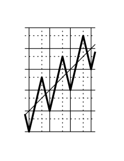
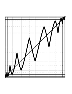
Figure 5. The constant slope map $F:\mathbb{R}\to\mathbb{R}$ and the conjugate map $f:[0,1]\to[0,1]$ with fixed points at $0,1$.

We enumerate the $P$-basic intervals as follows:

(14) $$I_{2k}=[h^{-1}(k),h^{-1}(k+b)],\quad I_{2k+1}=[h^{-1}(k+b),h^{-1}(k+1)],\quad k\in\mathbb{Z}.$$

The Markov transitions are given by

(15) $$f(I_{2k})=\bigcup\limits_{i=2k-2}^{2k+2}I_{i},\quad f(I_{2k+1})=\bigcup\limits_{i=2k}^{2k+2}I_{i},\quad k\in\mathbb{Z}.$$

We must verify that $f$ is mixing. Let $U,V$ be any pair of nonempty open intervals. We may assume that the points $0,1$ do not belong to $U$ or $V$. Passing through the conjugacy, we may work instead with the map $F$ and the intervals $h(U),h(V)$. Each iterated image of $h(U)$ that contains at most one folding point of $F$ is expanded in length by a factor of at least $\frac{1}{2}(2+\sqrt{5})>1$. Therefore some iterated image of $h(U)$ contains an entire $h(P)$-basic interval. The Markov transitions are such that the iterated images of an arbitrary basic interval eventually include any other given basic interval. This establishes the mixing property.

Let $T$ be the 0-1 transition matrix for the map $f$ and the partition set $P$. In light of Theorem 3.1, we wish to find all nonnegative solutions $v\in\mathbb{R}^{\mathcal{B}(P)},\lambda>1$ to the equation $Tv=\lambda v$. Comparing equation (15) with the definition of $T$, we are looking for all nonnegative solutions to the infinite system of equations

(16) $$\left\{\begin{array}[]{lcl}\lambda\,v_{I_{2k}}&=&\sum_{i=2k-2}^{2k+2}v_{I_{i}}\\ \lambda\,v_{I_{2k+1}}&=&\sum_{i=2k}^{2k+2}v_{I_{i}}\\ \end{array}\right.\qquad\qquad k\in\mathbb{Z}$$

Adding and subtracting equations, we obtain

$$\left\{\begin{array}[]{l}\lambda(v_{I_{2k+1}}+v_{I_{2k-1}}-v_{I_{2k}})=v_{I_{2k}}\\ \lambda v_{I_{2k+1}}=v_{I_{2k}}+v_{I_{2k+1}}+v_{I_{2k+2}}\end{array}\right.\qquad\qquad k\in\mathbb{Z}.$$

Solving for later variables in terms of earlier ones, we obtain

(17) $$\left[\begin{array}[]{c}v_{I_{2k+1}}\\ v_{I_{2k+2}}\end{array}\right]=\underbrace{\left[\begin{array}[]{cc}-1&1+\frac{1}{\lambda}\\ -\lambda+1&\lambda-1-\frac{1}{\lambda}\end{array}\right]}_{M_{\lambda}}\left[\begin{array}[]{c}v_{I_{2k-1}}\\ v_{I_{2k}}\end{array}\right]\qquad\qquad k\in\mathbb{Z}.$$

Equation (17) should be regarded as a linear recurrence relation on $v$. Notice (miracle) that $\det M_{\lambda}=1$ is independent of $\lambda$. Using the invertibility of $M_{\lambda}$, we may conclude inductively that

$$\left[\begin{array}[]{c}v_{I_{2k+1}}\\ v_{I_{2k+2}}\end{array}\right]=M_{\lambda}^{k}\left[\begin{array}[]{c}v_{I_{1}}\\ v_{I_{2}}\end{array}\right],\quad k\in\mathbb{Z}.$$

We may regard the matrix $M_{\lambda}$ as defining a dynamical system on $\mathbb{R}^{2}$. Then the entries of $v$ are the orbit of the initial point $(v_{I_{1}},v_{I_{2}})$. To obtain nonnegative entries for $v$, we must choose the initial point so that the whole orbit (both forward and backward) remains in the first quadrant. We can solve this problem using the elementary theory of linear transformations on $\mathbb{R}^{2}$. There are 3 cases we must consider – they are pictured in Figure 6 and explained in the following three paragraphs.

Figure 6. The action of $M_{\lambda}$ on $\mathbb{R}^{2}$

.

If $1<\lambda<2+\sqrt{5}$, then the eigenvalues of $M_{\lambda}$ are complex conjugates and $M_{\lambda}$ “rotates” $\mathbb{R}^{2}$ about the origin. In this case, no orbit stays in the first quadrant. The diligent reader may verify the implications $v_{I_{1}}\geq v_{I_{2}}\geq 0\implies v_{I_{4}}<0$ and $v_{I_{2}}\geq v_{I_{1}}\geq 0\implies v_{I_{-1}}<0$.

If $\lambda=2+\sqrt{5}$, then $M_{\lambda}$ has unique real eigenvalue $1$ with algebraic multiplicity 2 and geometric multiplicity 1. Thus, $M_{\lambda}$ acts as a shear on $\mathbb{R}^{2}$ parallel to a line of fixed points (corresponding to the unique eigenvector of $M_{\lambda}$). The only way to obtain a whole orbit in the first quadrant is to choose the initial point $(v_{I_{1}},v_{I_{2}})$ from the line of fixed points. This yields (up to a scalar multiple) the unique nonnegative solution

(18) $$v_{I_{2k}}=2,\quad v_{I_{2k+1}}=\sqrt{5}-1,\quad k\in\mathbb{Z}$$

Applying Theorem 3.1, we recover (up to scaling, and with fixed points at $\pm\infty$) the constant slope map $F$ which started our whole discussion.

If $\lambda>2+\sqrt{5}$, then $M_{\lambda}$ has distinct positive, real eigenvalues whose product is $1$. There are distinct eigenvectors in the first quadrant and the origin is a saddle fixed point. Any initial point $(v_{I_{1}},v_{I_{2}})$ chosen between these eigendirections in the first quadrant yields an unsummable, nonnegative $v$. We can achieve unsummability of $v$ on one side or on both sides, according as we choose the initial point to lie on one of these eigendirections or strictly between them. Accordingly, Theorem 3.1 yields a constant slope map either on an extended half line or on the extended real line, (see Remark 4.2).

10. No Constant Slope

We construct now a topologically mixing map $f\in\mathcal{CPMM}$ whose transition matrix does not admit any nonnegative eigenvectors, summable or otherwise. That means that $f$ is not conjugate to any map of any constant slope, even allowing for maps on the extended real line. In terms of the Vere-Jones recurrence hierarchy, our map $f$ has transient Markov dynamics. Indeed it must, since for recurrent Markov chains there always exists a nonnegative eigenvector (see [12]). For transient Markov chains, Pruitt [9] offers a nice criterion for the existence or nonexistence of a nonnegative eigenvector; our example was inspired by Pruitt’s paper. Other examples of this type are considered in the forthcoming article [3].

We construct $f$ as follows. Fix a subset $N\subset\mathbb{N}$, $1\notin N$, such that $\frac{\pi(n)}{n}\to 0$, and $\sum_{n=0}^{\infty}3^{-\pi(n)}<3$, where $\pi(n)=\#N\cap\{1,2,\ldots,n\}$, $\pi(0)=0$. If we wish to be explicit, we may take $N$ such that $\{\pi(n)\}_{n=0}^{\infty}$ is the sequence 0, 0, 1, 2, 2, 3, 3, 3, 4, 4, 4, 4, …. Subdivide $[0,1]$ into adjacent intervals $I_{n}=\left[\frac{1}{2^{n+1}},\frac{1}{2^{n}}\right]$, $n\geq 0$. Let $f:[0,1]\to[0,1]$ be the continuous, piecewise affine map with the following properties. For $n\in N$, $f$ maps $I_{n}$ onto $I_{n-1}$ once with slope $+2$. For $n\in\mathbb{N}\setminus N$ $f$ maps $I_{n}$ onto $I_{n-1}$ three times with alternating slopes $\pm 6$. Finally, $f$ maps $I_{0}$ onto the whole space $[0,1]$ with slope $-2$. The idea is illustrated in Figure 7; the choice of $N$ controls which windows contain only one branch of monotonicity.

Figure 7. A map not conjugate to any constant slope map.

If we further subdivide each of the intervals $I_{n}$, $n\geq 1$, into three subintervals $I_{n}^{k}=[\frac{1}{2^{n+1}}+\frac{k}{3\cdot 2^{n+1}},\frac{1}{2^{n+1}}+\frac{k+1}{3\cdot 2^{n+1}}]$, $k\in\{0,1,2\}$, then our map $f$ is countably piecewise monotone and Markov with respect to this refined partition.

We wish to use Theorem 3.1, and therefore we must verify that $f$ is topologically mixing. Let $U$ be an arbitrary open interval. If an interval is mapped forward monotonically by $f$, then its image is an interval of at least twice the length. Therefore, there is some minimal $n_{0}$ such that $f^{n_{0}}(U)$ contains a folding point of $f$. Then $f^{n_{0}+1}(U)$ contains a point of the form $2^{-n_{1}}$. Thus, $f^{n_{0}+n_{1}+2}(U)$ contains a neighborhood of zero, and hence a whole interval $I_{n_{2}}$. Then $f^{n_{0}+n_{1}+n_{2}+3}(U)=[0,1]$. This shows that $f$ is topologically mixing (and even locally eventually onto).

We investigate now the existence of nonnegative eigenvectors for the corresponding transition matrix. Suppose that there is an eigenvector with some eigenvalue $\lambda>0$. Let $v_{n}$ denote the sum of the entries corresponding to $I_{n}^{1}$, $I_{n}^{2}$, and $I_{n}^{3}$, and let $v_{0}$ denote the entry corresponding to the undivided interval $I_{0}$. Then the eigenvector condition implies that

(19) $$\lambda v_{n}=\begin{cases}v_{n-1},&\textnormal{if }n\in N\\ 3v_{n-1},&\textnormal{if }n\notin N\end{cases},\qquad\lambda v_{0}=\sum_{n=0}^{\infty}v_{n}.$$

By rescaling our vector if necessary, we may suppose that $v_{0}=1$. It follows inductively that $v_{n}=\frac{3^{n-\pi(n)}}{\lambda^{n}}$. If $\lambda\geq 3$, then $\sum_{n=0}^{\infty}v_{n}\leq\sum_{n=0}^{\infty}3^{-\pi(n)}<3$ by the choice of $N$, which contradicts the last equation of (19). If $\lambda<3$, then $v_{n}\to\infty$ by the choice of $N$, so that $\sum_{n}v_{n}$ diverges, which again contradicts (19). It follows that our transition matrix has no nonnegative eigenvectors. In light of Theorem 3.1, this means that there does not exist any conjugate map of any constant slope, even allowing for maps on the extended real line.

11. Piecewise Continuous Case

We turn our attention now to piecewise continuous maps. We finish the proof of Theorem 3.2, showing by example the insufficiency of condition (2). We begin by defining two maps $f$, $g$ on the extended half-line $[0,\infty]$ with the same Markov structure. The $P$-basic intervals are the intervals $A_{i}=\left(2^{i}+2i-3,2^{i+1}+2i-2\right)$, $B_{i}=\left(2^{i+1}+2i-2,2^{i+1}+2i-1\right)$, $i=0,1,2,\ldots$; thus $P$ is the set of endpoints of these intervals together with the point at infinity. Notice that these intervals have lengths $|A_{i}|=2^{i}+1$, $|B_{i}|=1$ and are arranged from left to right in the order $A_{0}<B_{0}<A_{1}<B_{1}<A_{2}<B_{2}<\ldots$. Both maps $f$, $g$ will exhibit Markov transitions as indicated in Figure 8, where an arrow $I\to J$ indicates that the image of interval $I$ includes interval $J$.

Figure 8. Transition diagram for the maps $f$ and $g$.

For each $i$, both $g|_{A_{i}}$ and $g|_{B_{i}}$ are affine with slope $2$; this completes the definition of $g$. Moreover, for all $i$, $f|_{B_{i}}$ is affine with slope $2$. However, the definition of $f|_{A_{i}}$ is different. For each $i$, $f$ carries $\left(2^{i}+2i-3,2^{i+1}+2i-3\right)$ (all but the right-most unit of $A_{i}$) affinely onto $B_{i}$ with slope $2^{-i}$, and carries $\left(2^{i+1}+2i-3,2^{i+1}+2i-2\right)$ (the right-most unit of $A_{i}$) affinely onto $A_{i+1}$ with slope $2^{i+1}+1$. This completes the definition of $f$. The graphs of both maps are shown below.

Figure 9. The graphs of the maps $f$ and $g$.

We claim that the map $f$ is topologically mixing. Indeed, let $U,V\subset[0,\infty]$ be any open intervals. If for each $i$, $f^{i}(U)$ is contained in a single $P$-basic interval, then either there are infinitely many indices $i_{j}$ for which $f^{i_{j}}(U)\subset A_{0}$ or there are only finitely many (perhaps zero). The first case is impossible because the length $|f^{i_{j+1}}(U)|$ must be greater than the length $|f^{i_{j}}(U)|$ by a factor of at least $2$ (consider all possible loops from $A_{0}$ to itself in Figure 8 and multiply slopes along the loop). The second case is impossible because then some image of $U$ must be contained in a set of the form $\bigcap_{k=0}^{\infty}f^{-k}(A_{n+k})$ for some $n$ (look again at Figure 8). But the length of the finite intersection $\bigcap_{k=0}^{K}f^{-k}(A_{n+k})$ is equal to the length of $A_{n}$ times the proportion of $A_{n}$ mapped onto $A_{n+1}$, times the proportion of $A_{n+1}$ mapped onto $A_{n+2}$, and so on, up to the proportion of $A_{n+K-1}$ mapped onto $A_{n+K}$, that is,

(20) $$\left|\bigcap_{k=0}^{K}f^{-k}A_{n+k}\right|=|A_{n}|\times\frac{1}{|A_{n}|}\times\frac{1}{|A_{n+1}|}\times\cdots\times\frac{1}{|A_{n+K-1}|}=\\ =\frac{2^{n}+1}{\left(2^{n}+1\right)\left(2^{n+1}+1\right)\cdots\left(2^{n+K-1}+1\right)}$$

which decreases to zero as $K\to\infty$. We conclude that there exists $i$ such that $f^{i}(U)$ is not contained in a single $P$-basic interval. Looking now at the graph of $f$, we can see that either $f^{i+1}(U)$ or else $f^{i+2}(U)$ contains some interval $(0,\varepsilon)$, and in particular, contains some interval $(0,2^{-i^{\prime}})$. Observe that $f^{2i^{\prime}}(0,2^{-i^{\prime}})=A_{0}$. Let $i^{\prime\prime}$ be such that $V\cap(A_{i^{\prime\prime}}\cup B_{i^{\prime\prime}})\neq\emptyset$. For all $n\geq i^{\prime\prime}+3$ we have $f^{n}(A_{0})\supset(A_{i^{\prime\prime}}\cup B_{i^{\prime\prime}})$ (look again for paths in Figure 8). Therefore, for all $n\geq i+2+2i^{\prime}+i^{\prime\prime}+3$ we have $f^{n}(U)\cap V\neq\emptyset$. This concludes the proof that $f$ is topologically mixing.

Next we consider eigenvectors associated with the Markov structure of the map $f$. We single out the eigenvalue $\lambda=2$, and we denote by $a_{i},b_{i}$, $i=0,1,2,\ldots$, the entries of an eigenvector corresponding to the intervals $A_{i},B_{i}$, $i=0,1,2,\ldots$, respectively. In particular, we must find nonnegative solutions to the infinite system of equations

$$\left\{\begin{array}[]{l}2a_{i}=b_{i}+a_{i+1}\\ 2b_{i}=a_{0}\end{array}\right.,\qquad i\in\mathbb{N}.$$

Since eigenvectors are defined only up to a scaling constant, we are free to fix $b_{0}=1$. It follows that $a_{0}=2$ and that $b_{i}=1$ for all $i$. Then the entries $a_{i}$ can be computed inductively as $a_{i}=2^{i}+1$. Up to scaling, this is the only eigenvector for the eigenvalue $\lambda=2$.

Despite the existence of this eigenvector, $f$ is not conjugate to any map of constant slope $2$. Indeed, let $\varphi$ be a homeomorphism of $[0,\infty]$ onto a closed (sub)interval of the extended real line; without loss of generality we may assume that $\varphi$ is orientation-preserving. Suppose that the conjugate map $\varphi\circ f\circ\varphi^{-1}$ has constant slope $2$. By Lemma 4.1 the lengths of the $\varphi(P)$-basic intervals must be given by an eigenvector with eigenvalue $2$. Therefore, after rescaling and translating $\varphi$ if necessary, the map $\varphi\circ f\circ\varphi^{-1}$ is equal to the map $g$ which we have already defined, so that $\varphi(A_{i})=A_{i}$ and $\varphi(B_{i})=B_{i}$ for all $i$. In other words, $\varphi$ fixes the entire set $P$. Let $x_{k}$ denote the left-hand endpoint of the interval $A_{0}\cap f^{-1}(A_{1})\cap\ldots\cap f^{-k}(A_{k})$, and let $y_{k}$ denote the left-hand endpoint of the interval $A_{0}\cap g^{-1}(A_{1})\cap\ldots\cap g^{-k}(A_{k})$. Since $\varphi$ conjugates $f$ with $g$, we must have $\varphi(x_{k})=y_{k}$ for all $k$. By the same reasoning as we used to derive equation (20), we have

$$\begin{array}[]{l}x_{k}=2-2\times\frac{1}{2}\times\frac{1}{3}\times\cdots\times\frac{1}{2^{k-1}+1},\\ y_{k}=2-2\times\frac{3}{4}\times\frac{5}{6}\times\cdots\times\frac{2^{k}+1}{2^{k}+2}.\end{array}$$

Inductively, $y_{k}=2-\frac{2^{k}+1}{2^{k}}$. We have $x_{k}\to 2$ and $y_{k}\to 1$. Since $\varphi(2)=2$, this contradicts the continuity of $\varphi$. We conclude that $f$ is not conjugate to any map of constant slope $2$.

Remark 11.1.

We can also interpret this example from the point of view of wandering intervals. The map $g$ has a wandering interval $A_{0}\cap g^{-1}(A_{1})\cap g^{-2}(A_{2})\cap\cdots$. Thus, even though it has constant slope $2$ and the right Markov structure, it cannot be conjugate to the topologically mixing map $f$.

12. The Mixing Hypothesis

We turn our attention now to maps which are topologically transitive but not topologically mixing. We finish the proof of Theorem 3.3, showing the insufficiency of condition (2). We construct a map $\tilde{f}$ in $\mathcal{CPMM}$ which is topologically transitive but not mixing. We give a nonnegative eigenvector $v$ for the transition matrix $T$, but prove that $\tilde{f}$ is not conjugate to any map on any subinterval $[a,b]\subset[-\infty,\infty]$ with constant slope equal to the eigenvalue of $v$.

Let $f$ and $P$ be as defined in Section 9. We define $\tilde{f}:[-1,1]\to[-1,1]$ by the formula

$$\tilde{f}(x)=\begin{cases}-f(x),&\textnormal{ if }x\in[0,1]\\ -x&\textnormal{ if }x\in[-1,0]\end{cases}$$

This map $\tilde{f}$ is piecewise monotone and Markov with respect to the set $\tilde{P}=P\cup-P$. Figure 10 shows the graph of $\tilde{f}$ (in bold). Superimposed is the graph of the second iterate $\tilde{f}^{2}$. By construction, $\tilde{f}^{2}|_{[0,1]}$ and $\tilde{f}^{2}|_{[-1,0]}$ are both isomorphic copies of the map $f$. In this sense, $\tilde{f}$ is a kind of dynamical square root of $f$.

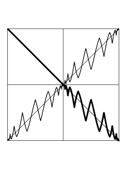
Figure 10. The map $\tilde{f}$ (shown in bold) is transitive but not mixing. It’s second iterate (superimposed) consists of two copies of the map $f$ from Section 9 (compare with Figure 5).

We claim that $\tilde{f}$ is topologically transitive, but not topologically mixing. To see the transitivity, take arbitrary nonempty open subsets $U$, $V$ of $[-1,1]$. After shrinking these sets, we may assume that $U,V$ are open intervals not containing $0$. Consider first the case when $U,V\subset[0,1]$. By the transitivity of $f$ there exists $n$ such that $U\cap f^{-n}(V)\neq\emptyset$, but then $U\cap\tilde{f}^{-2n}(V)\neq\emptyset$. The case when $U,V\subset[-1,0]$ is similar. Now consider the case when $U\subset[0,1]$ and $V\subset[-1,0]$. Using the reflected set $-V$ and the transitivity of $f$, find $n$ such that $U\cap f^{-n}(-V)\neq\emptyset$. Then $U\cap\tilde{f}^{2n-1}(V)\neq\emptyset$. The case when $U\subset[-1,0]$ and $V\subset[0,1]$ is similar. This shows topological transitivity of $\tilde{f}$. To see that $\tilde{f}$ is not topologically mixing, notice that the set $\{n\in\mathbb{N}:(0,1)\cap\tilde{f}^{-n}(0,1)\neq\emptyset\}$ consists of only the even natural numbers.

Let $\tilde{T}$ be the 0-1 transition matrix for the map $\tilde{f}$ with respect to the Markov partition by $\tilde{P}$. We label the $\tilde{P}$-basic intervals $I_{k},J_{k},k\in\mathbb{Z}$, where the intervals $I_{k}$ are given by equation (14) and the intervals $J_{k}$ are their reflections, $J_{k}=-I_{k}$. Fix $\lambda=2+\sqrt{5}$. We find all nonnegative solutions $v\in\mathbb{R}^{\mathcal{B}(\tilde{P})}$ to the equation $\tilde{T}v=\sqrt{\lambda}v$. In light of the Markov transitions, this is the infinite system of equations

(21) $$\left\{\begin{array}[]{lcl}\sqrt{\lambda}\,v_{I_{2k}}&=&\sum_{i=2k-2}^{2k+2}v_{J_{i}}\\ \sqrt{\lambda}\,v_{I_{2k+1}}&=&\sum_{i=2k}^{2k+2}v_{J_{i}}\\ \sqrt{\lambda}\,v_{J_{k}}&=&v_{I_{k}}\end{array}\right.\qquad\qquad k\in\mathbb{Z}$$

If we substitute the last line in equation (21) into the first two lines, we recover equation (16), which for $\lambda=2+\sqrt{5}$ has (up to scalar multiples) the unique nonnegative solution (18). Therefore (21) has (up to scalar multiples) the unique nonnegative solution

(22) $$v_{I_{2k}}=2,\quad v_{I_{2k+1}}=\sqrt{5}-1,\quad v_{J_{2k}}=\frac{2}{\sqrt{\lambda}},\quad v_{J_{2k+1}}=\frac{\sqrt{5}-1}{\sqrt{\lambda}},\qquad k\in\mathbb{Z}.$$

Now we show that despite the existence of this eigenvector $v$, there does not exist any conjugacy $\psi$ of the map $\tilde{f}$ to a map of constant slope $\sqrt{\lambda}$. Assume the contrary. Then by the uniqueness of $v$ and by Lemma 4.1, we have

$$|\psi(I_{2k})|=2c,\quad|\psi(I_{2k+1})|=(\sqrt{5}-1)c,\\ |\psi(J_{2k})|=\frac{2c}{\sqrt{\lambda}},\quad|\psi(J_{2k+1})|=\frac{(\sqrt{5}-1)c}{\sqrt{\lambda}},\qquad k\in\mathbb{Z},$$

for some positive real scalar $c$. But the $P$-basic intervals accumulate at the center of $[-1,1]$ so that a small open interval $(-\varepsilon,\varepsilon)$ contains infinitely many $P$-basic intervals. Thus, $\psi(-\varepsilon,\varepsilon)$ has infinite length. On the other hand, a nondecreasing homeomorphism $\psi:[-1,1]\to[-\infty,\infty]$ must take finite values at every interior point of the interval $[-1,1]$. This is a contradiction.

References

- [1] Ll. Alsedà, J. Llibre and M. Misiurewicz, Combinatorial Dynamics and Entropy in Dimension One, 2nd edition, Advanced Series in Nonlinear Dynamics 5, World Scientific, Singapore, 2000.
- [2] J. Bobok, Semiconjugacy to a map of a constant slope, Studia Math. 208 (2012), 213–228.
- [3] J. Bobok and H. Bruin, Conjugacy to a map of constant slope II, Preprint: arXiv:1602.06905.
- [4] J. Bobok and M. Soukenka, On piecewise affine interval maps with countably many laps, Discrete Cont. Dyn. Syst. 31(3) (2011), 753–762
- [5] J. Milnor and W. Thurston, On iterated maps of the interval, in Dynamical Systems, Lecture Notes in Math. 1342, Springer, Berlin, 1988, 465–563.
- [6] M. Misiurewicz, Absolutely continuous measures for certain maps of an interval, Publ. Math. IHES 53 (1981), 17–51.
- [7] M. Misiurewicz and S. Roth, No semiconjugacy to a map of constant slope, Ergodic Theory Dynam. Systems, available on CJO2014. doi:10.1017/etds.2014.81.
- [8] W. Parry, Symbolic dynamics and transformations of the unit interval, Trans. Amer. Math. Soc. 122 (1966), 368–378.
- [9] W. Pruitt, Eigenvalues of nonnegative matrices, Ann. Math. Statist. 35 (1964) 1797–1800.
- [10] S. Ruette, On the Vere-Jones classification and existence of maximal measures for countable topological Markov chains Pacific J. Math. 209(2) (2003), 366–380.
- [11] D. Vere-Jones, Ergodic properties of nonnegative matrices-I, Pacific J. Math. 22(2) (1967), 361–386.
- [12] D. Vere-Jones, Geometric ergodicity in denumerable Markov chains, Quart. J. Math. Oxford Ser. (2), 13 (1962), 7–28.