Effective cosmological constant induced by stochastic fluctuations of Newton’s constant

Abstract

We consider implications of the microscopic dynamics of spacetime for the evolution of cosmological models. We argue that quantum geometry effects may lead to stochastic fluctuations of the gravitational constant, which is thus considered as a macroscopic effective dynamical quantity. Consistency with Riemannian geometry entails the presence of a time-dependent dark energy term in the modified field equations, which can be expressed in terms of the dynamical gravitational constant. We suggest that the late-time accelerated expansion of the Universe may be ascribed to quantum fluctuations in the geometry of spacetime rather than the vacuum energy from the matter sector.

It is unlikely that the geometry of spacetime remains unchanged all the way to microscopical scales, smaller than the Panck’s length $l_{\rm Pl}=\sqrt{\hbar G_{\rm N}/c^{3}}$, where quantum effects can no longer be neglected and geometry may altogether lose the meaning we are familiar with. The spacetime structure at microscopic scales is of course not known, although some indications from Noncommutative Geometry Connes ; WSS , String Theory String , or Loop Quantum Gravity LQG are available. Even though a full theory of quantum spacetime is not yet available, it is reasonable to assume that Einstein’s equations (as well as the ones of quantum field theory) will be substituted by a new set of relations. We may in the meantime try to surmise some sort of effects which could be the outcome of the quantum substructure. The aim of this paper is to investigate the possibility that the coupling between matter and the gravitational field varies in a random way, possibly due to quantum gravitational effects.

The variability of fundamental constants is an old idea which goes back to Dirac Dirac , and it would be a clear indication of new physics. In fact, the variation of fundamental constants would entail a violation of the Equivalence Principle Uzan ; Will and could not find an explanation within the same framework where those constants belong. In the language of effective field theories, such constants would be replaced by new (scalar) fields obeying their own dynamics Uzan , as for instance in the framework of Brans-Dicke theory BransDicke (or more general scalar-tensor theories of gravity), where the gravitational constant is determined by the vacuum expectation value of the dilaton. Clearly, in this framework the variation of fundamental constants must be slow enough, both in space and time, so as to guarantee the reproducibility of the experiments performed so far. The possibility of measuring such variations, as well as the theoretical reasons for introducing such dimensionful quantities in first place, are actually delicate issues that have generated debate in the community. Interested readers are referred to e.g. Refs. Duff ; Trialogue . We will see in the following that the variability of the coupling, which can be expressed in a unit independent fashion in terms of dimensionless quantities, is the physically relevant (and measurable) quantity. While most of the theoretical work on variable constants has been on a more or less regular variability on cosmological scales, the motivations of this work point to a stochastic variability on very short scales, typically Planckian. Thus, it is in general conceivable that $G_{\rm N}$ could not be a constant at the outset but instead it must be determined from the microscopic dynamics, hence in principle it can be affected by the collective behaviour of spacetime quanta. Analogous considerations apply to $\hbar$ ManganoLizziPorzio for the effects induced by its stochastic fluctuations on nonrelativistic quantum systems. In fact, it is a general property of quantum systems that fast degrees of freedom can be approximated by stochastic noise, see Ref. book noise . In the following, we assume that the effects of the underlying microscopic dynamics of spacetime can be given an effective classical description by means of a stochastic gravitational constant. The fluctuations and the typical time scale of the stochastic process must be suitably small, e.g. ${\cal{O}}(t_{\rm Pl})$, to ensure that there is no contradiction with observations. A fluctuating gravitational background can induce the Higgs mass term as well Kurkov .

Newton’s gravitational constant appears in the fundamental equation of Einstein’s theory of General Relativity

$$G_{ab}=8\pi G_{\rm N}\;T_{ab}~{}.$$ (1)

We take Eq. (1) as a starting point and work out the consequences of having a dynamical $G_{\rm N}$. Turning $G_{\rm N}$ naively into a dynamical variable, while keeping $T_{ab}$ covariantly conserved, would result into a violation of the Bianchi identities, as pointed out already in Ref. Fritzsch .

$$0=\nabla^{a}G_{ab}=8\pi\nabla^{a}(G_{\rm N}T_{ab})~{}.$$ (2)

The solution to the impasse is to split the energy-momentum tensor into a matter term, which satisfies the usual conservation law, and a correction term such that Eq. (2) is satisfied:

$$T_{ab}=T^{\rm matter}_{ab}+\tau_{ab}~{}.$$ (3)

In a isotropic and homogeneous cosmological model, we have

$$T^{\rm matter}_{ab}=(\rho+p)u_{a}u_{b}+pg_{ab}~{},$$ (4)

where $u_{a}$ is tangent to the geodesic of a isotropic observer and the fluid satisfies the equation of state $p=w\rho$. A similar ansatz could be made for the extra term. However, since it represents the only part of the energy-momentum tensor that does not arise from the matter sector, it is quite natural to connect it to the only such form of energy there is evidence for, namely to dark energy. We therefore write

$$\tau_{ab}=-\lambda g_{ab}~{}.$$ (5)

In this way dark energy is naturally connected to the dynamics of $G_{\rm N}$, stemming from quantum gravitational effects. There is no need for other physical fields to be introduced in the theory. In contrast to Ref. Fritzsch , we are not trying to establish a connection with the matter sector in order to explain such variations. Rather, we argue that their origin is entirely due to quantum geometry effects. At the macroscopic level, these must be such that general covariance and the Bianchi identities are preserved. An extra constraint on the form of $\tau_{ab}$ comes from observations, which tell us that it has to satisfy Eq. (5). In the following we will consider just variation over time. This is to be considered a toy model of a full treatment for which variations are, always at Planckian scales, in both space and time.

The physical fluid satisfies the continuity equation

$$\dot{\rho}+3H(\rho+p)=0~{}.$$ (6)

The evolution of the time-dependent “cosmological constant” $\lambda$ is obtained from the Bianchi identities

$$\dot{G}_{\rm N}(\rho+\lambda)+G_{\rm N}\dot{\lambda}=0~{}.$$ (7)

The solution to this equation is

$$\lambda(t)=\frac{G_{\rm N}(t_{i})}{G_{\rm N}(t)}\left(\lambda(t_{i})-\int_{t_{i}}^{t}\mbox{d}t^{\prime}\;\frac{\dot{G}_{\rm N}(t^{\prime})}{G_{\rm N}(t_{i})}\rho(t^{\prime})\right)~{}.$$ (8)

By substituting Eq. (8) in the sources of the Friedmann equation we get

$$H^{2}(t)=\frac{8\pi}{3}\left(G_{N}(t_{i})\left(\rho(t_{i})+\lambda(t_{i})\right)+\int_{t_{i}}^{t}G_{N}\dot{\rho}\right)~{}.$$ (9)

Considering $t_{i}$ in the matter- or radiation-dominated era, $\lambda(t_{i})\ll\rho(t_{i})$ and we can safely neglect the second term in the r.h.s. of the above equation. Notice that in this case, Eq. (9) does not make any reference to $\lambda$, but all dark energy contributions are instead included in the time evolution of $G_{\rm N}$ via an integral operator.

By differentiating Eq. (9) and using Eq. (6), in the case of a Universe filled with non-relativistic matter ($w=0$), we get

$$\dot{H}=-4\pi G_{\rm N}\rho~{},$$ (10)

which together with Eq. (6) and the constraint on the initial conditions for $\rho$ and $H$, namely

$$H^{2}(t_{i})=\frac{8\pi}{3}G_{\rm N}(t_{i})\rho(t_{i})~{},$$ (11)

fully determines the dynamics. We can express

$$G_{\rm N}(t)=\overline{G}_{\rm N}(1+\sigma\xi(t))$$ (12)

as the sum of a constant background value and a perturbation. Note that the last equation still makes sense even if one assumes the point of view of Ref. Duff . In fact, once we introduce a units system, e.g. one such that $\overline{G}_{\rm N}=1$, Eq. (12) is equivalent to the statement that the r.h.s. of Einstein’s equations (1) has a nonstandard form, with new terms that can be expressed in terms of dimensionless quantities.

Let us rewrite Eq. (10) in a differential form, namely

$$\mbox{d}H=-4\pi\overline{G}_{\rm N}\rho(1+\sigma\xi(t))\mbox{d}t~{}.$$ (13)

Assuming that $\xi(t)$ has a white noise distribution, the last equation reads

$$\mbox{d}H=-4\pi\overline{G}_{\rm N}\rho(\mbox{d}t+\sigma\mbox{d}W_{t})~{},$$ (14)

where $W_{t}$ is a Wiener process. Loosely speaking the white noise is the derivative of the Wiener process and satisfies the properties

$$\langle\xi(t)\rangle = 0,$$ (15)

$$\langle\xi(t)\xi(t^{\prime})\rangle = \delta(t-t^{\prime})~{},$$ (16)

where $\langle~{}\rangle$ denotes an ensemble average. A mathematically more precise description of a stochastic process is given by considering a discrete time evolution and using the theory of stochastic integration Oksendal . Thus, Eq. (14) is interepreted as a Îto process. For the sake of simplicity we consider a partition of the interval $t_{i}\equiv t_{0}<t_{1}<\dots<t_{k}<\dots<t_{N}\equiv t$ with uniform time step $h$.

The Wiener process $W_{t}$ has the following properties:

• $W_{t_{i}}=0$ with probability $1$;

• The increments $W_{t_{k+1}}-W_{t_{k}}$ are statistically independent Gaussian variables with mean $0$ and variance $t_{k+1}-t_{k}=h$.

It plays the rôle of a stochastic driving term in Eq. (14).

We have investigated numerically the behaviour of the solutions for such a model with parameters $0\leq\sigma\leq 1$, $10^{-6}\leq h\leq 10^{-2}$, in units such that $\overline{G}_{N}=1$, for different choices of the initial condition $\rho(t_{i})$. Qualitatively the behaviour of the solutions is the same and is represented in Fig. 1 for a given path $W_{t}$, where the plot of the energy density $\rho(t)$ and the Hubble rate $H(t)$ is shown.

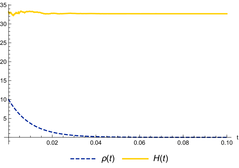
Figure 1: Plot of the solution of the model (6), (11), (14), for the particular choice of parameters $\sigma=0.1$, $\rho_{0}=10$ and time step $h=10^{-4}$, in units such that $\overline{G}_{\rm N}=1$. The horizontal asymptote of $H(t)$ for $t\to\infty$ corresponds to a late era of accelerated expansion, when the Universe is dominated by a “cosmological constant”. Stochastic noise has an effect which is relevant at early times, whereas it is negligible at late times since it is suppressed by the small value of the energy density, as one can also see from (14). The qualitative behaviour of the solutions is a general feature, which does not depend on the particular choice of parameters.

As $t\to\infty$, $\rho$ decays as in standard cosmology, while $H$ attains a nonvanishing positive limit. The value of the asymptotic limit does not vary much with the random sequence, and is not particularly sensitive to the parameters. Since we are dealing with a simplified model this semi qualitative analysis is sufficient. This implies an exponential expansion at late times without the need to introduce a cosmological constant by hand or to originate it from the matter sector, e.g. as vacuum energy. Note that this is a general feature of the model that does not depend on the particular values chosen for $\rho_{0}$ or the noise strength $\sigma$. Furthermore, when $\sigma=0$ one recovers the standard cosmology in the matter-dominated era, namely $\rho\propto 1/t^{2}$ and $H\propto 1/t$.

The effective cosmological constant in the r.h.s. of Eq. (9) is given by the formula

$$\Lambda_{\rm eff}(t)=\sigma\left(\xi(t_{i})\rho(t_{i})+\int_{t_{i}}^{t}\dot{\rho}\;\mbox{d}W_{t}\right)~{},$$ (17)

where the second term is a stochastic integral. The first term dominates over the second with probability close to $1$, as shown in the following. Hence, when the first step of the random walk is positive, the Universe is exponentially expanding at late times, whereas for a negative initial step $H$ takes large negative values. We are therefore led to assume the initial condition

$$\xi(t_{i})>0~{},$$ (18)

which guarantees the stability of the Universe and is compatible with the observed accelerated expansion.

We compute the probability to observe a negative value of the effective cosmological constant given the initial condition on the noise (18). This actually forces the first step of the random walk to follow a half-normal distribution, whereas all the other steps of the random walk are normally distributed, as it is customary. Using the statistical properties of the increments of the Wiener process $W_{t}$ one finds

$$\left\langle\frac{\Lambda(t)}{\sigma}\right\rangle = \left\langle\frac{W_{t_{i}}}{h}\right\rangle\rho(t_{i})=\sqrt{\frac{2}{\pi h}}\rho(t_{i})$$ (19)

$$\left\langle\frac{\Lambda^{2}(t)}{\sigma^{2}}\right\rangle = \left\langle\left(\frac{W_{t_{i}}}{h}\right)^{2}\right\rangle\rho^{2}(t_{i})+\sum_{k}(\rho^{\prime}(t_{k}))^{2}h+2\rho(t_{i})\rho^{\prime}(t_{i})$$ (20)

$$\approx \left\langle\left(\frac{W_{t_{i}}}{h}\right)^{2}\right\rangle\rho^{2}(t_{i})=\frac{\rho^{2}(t_{i})}{h}$$

Therefore the value $\Lambda=0$ is $x$ standard deviations away from its mean value, with

$$x=\sqrt{\frac{2\pi}{\pi-2}}.$$ (21)

Hence, the probability of observing a non-positive value of $\Lambda$ (leading to a collapsing Universe) is $\lesssim 0.0095$, regardless of the initial condition, the noise strength $\sigma$ and the time step. In a more complete treatment which may take also space variation into account, these unstable cases will anyway not be a problem, since the instabilities will be just covered by the expanding areas.

Considering a Universe with more than one matter component, the effective cosmological constant receives contribution from each of them, with the dominant contribution still coming from the initial value of the white noise $\xi(t_{i})$ multiplied by the total energy density as in (17). In other words, the effective cosmological constant depends on the initial value of the total energy density, but not on the species populating the Universe. It seems natural to fix the initial data at a time where all species where equally dominating, i.e. $t_{i}\approx t_{\rm Pl}$. This conclusion, if correct, due to the limits of our effective approach at Planckian times, implies that the final stage of evolution of the Universe is entirely determined by quantum fluctuations of the spacetime geometry at early times. Furthermore, being determined only by the initial value of the total energy density, it treats all fields on the same level and it is insensitive to further details of the Universe’s history. In this sense Eq. (18) can be interpreted as a constraint on the underlying quantum theory, at the time when the dynamics of the fast degrees of freedom of the gravitational field approach their stochastic limit.

I Outlook and conclusions

Within an effective macroscopic description of the dynamics of the gravitational field, we have considered a stochastically fluctuating gravitational constant as a possible phenomenological feature of a theory of quantum gravity. Consistency with the Bianchi identities requires the addition of an extra source term, which does not communicate with the matter sector and may be interpreted as dark energy. We built a simple model where the latter is seen to be responsible for the present acceleration in the expansion of the Universe, which is thus seen to have a purely quantum geometrical origin. The simplifications introduced in the model and the sensitivity of the effective cosmological constant to the value of the total energy density at the Planck time prevent us from using such model to extract quantitative predictions for the present value of the cosmological constant and its probability. It is our hope that this preliminary work could open new ways towards a solution to the cosmological constant problem.

If the picture obtained from our model could be consistently obtained from a fundamental theory of quantum gravity, it would show that quantum gravitational phenomena are already being observed in the Universe today when looking at the acceleration of its expansion rate. Moreover, it would provide indirect evidence for the variation over time of the gravitational constant. More work has to be done in order to gain a better understanding of the rôle played by the initial conditions on the energy content of the Universe, since the cosmological constant obtained from our toy model seems to have a strong dependence on them.

Acknowledgments This article is based upon work from COST Action MP1405 QSPACE, supported by COST (European Cooperation in Science and Technology). M.d.C. would like to thank Tobias Hartung for helpful discussions. M.d.C. and F.L. also thank G.Mangano for useful discussions. F.L. is supported by INFN, I.S.’s GEOSYMQFT and received partial support by CUR Generalitat de Catalunya under projects FPA2013-46570 and 2014 SGR 104, MDM-2014-0369 of ICCUB (Unidad de Excelencia ‘Maria de Maeztu’).

References

- (1) A. Connes, “Noncommutative geometry year 2000”, Birkh user Basel (2000).
- (2) P. Aschieri, M. Dimitrijevic, P. Kulish, F. Lizzi and J. Wess, “Noncommutative spacetimes: Symmetries in noncommutative geometry and field theory,” Lect. Notes Phys. 774 (2009) 1.
- (3) J. Polchinski, “String theory: Volume 2, superstring theory and beyond”, Cambridge university press (1998)
- (4) C. Rovelli, Loop quantum gravity: the first twenty five years. Class. Quant. Grav. 28, 153002 (2011). [arXiv:1012.4707 [gr-qc]].
- (5) P.A.M. Dirac, “The Cosmological Constants.” Nature 139 , 323 (1937).
- (6) J. P. Uzan, “Varying Constants, Gravitation and Cosmology,” Living Rev. Rel. 14, 2 (2011) doi:10.12942/lrr-2011-2 [arXiv:1009.5514 [astro-ph.CO]].
- (7) C. M. Will, “Theory and experiment in gravitational physics,” Cambridge University Press (1993).
- (8) C. Brans and R. H. Dicke, “Mach’s principle and a relativistic theory of gravitation,” Phys. Rev. 124, 925 (1961). doi:10.1103/PhysRev.124.925
- (9) M. Duff, “How fundamental are fundamental constants?” Contemporary Physics 56, 35 (2015).
- (10) M. J. Duff, L. B. Okun and G. Veneziano, “Trialogue on the number of fundamental constants,” JHEP 0203, 023 (2002) doi:10.1088/1126-6708/2002/03/023 [physics/0110060].
- (11) G. Mangano, F. Lizzi and A. Porzio, “Inconstant Planck’s constant,” Int. J. Mod. Phys. A 30 (2015) 34, 1550209 doi:10.1142/S0217751X15502097 [arXiv:1509.02107 [quant-ph]].
- (12) L. Accardi, Y. G. Lu and I. Volovich, “Quantum theory and its stochastic limit,” Springer Science & Business Media (2013).
- (13) M. Kurkov, “Emergent spontaneous symmetry breaking and emergent symmetry restoration in rippling gravitational background,” arXiv:1601.00622 [hep-th].
- (14) H. Fritzsch and J. Sola, “Fundamental constants and cosmic vacuum: the micro and macro connection,” Mod. Phys. Lett. A 30, no. 22, 1540034 (2015) doi:10.1142/S0217732315400349 [arXiv:1502.01411 [gr-qc]].
- (15) B. Øksendal, “Stochastic differential equations: an introduction with applications,” Springer Science & Business Media (2013).