Analysis of Schwarz methods for a hybridizable discontinuous Galerkin discretization: the many subdomain case

Abstract.

Schwarz methods are attractive parallel solution techniques for solving large-scale linear systems obtained from discretizations of partial differential equations (PDEs). Due to the iterative nature of Schwarz methods, convergence rates are an important criterion to quantify their performance. Optimized Schwarz methods (OSM) form a class of Schwarz methods that are designed to achieve faster convergence rates by employing optimized transmission conditions between subdomains. It has been shown recently that for a two-subdomain case, OSM is a natural solver for hybridizable discontinuous Galerkin (HDG) discretizations of elliptic PDEs. In this paper, we generalize the preceding result to the many-subdomain case and obtain sharp convergence rates with respect to the mesh size and polynomial degree, the subdomain diameter, and the zeroth-order term of the underlying PDE, which allows us for the first time to give precise convergence estimates for OSM used to solve parabolic problems by implicit time stepping. We illustrate our theoretical results with numerical experiments.

1. Introduction

For the numerical treatment of a parabolic equation, e.g.,

(1.1) $$\begin{array}[]{rcll}\displaystyle\frac{\partial{u}}{\partial{t}}-\nabla\cdot(a(x)\nabla u)&=&f(x,t)&\textrm{in $\Omega\times(0,T]$},\\ u(x,t)&=&0&\textrm{on $\partial\Omega\times(0,T]$},\\ u(x,0)&=&g(x)&\textrm{on $\Omega$},\end{array}$$

one often first discretizes the spatial dimension using a finite difference (FD), finite element (FE) or discontinuous Galerkin (DG) method. This approach, called method of lines, results in a semi-discrete system where the unknown $u(x,t)$ is approximated by a finite dimensional vector ${\boldsymbol{u}}_{h}(t)$ and the differential operator $-\nabla\cdot(a(x)\nabla)$ by a stiffness matrix which we denote by $A_{h}$. More precisely we then have

(1.2) $$\frac{\partial{{\boldsymbol{u}}_{h}(t)}}{\partial{t}}+A_{h}{\boldsymbol{u}}_{h}(t)={\boldsymbol{f}}(t),$$

and ${\boldsymbol{u}}_{h}(t=0)={\boldsymbol{g}}_{h}$. We then discretize in time using for example a backward Euler method with time step $\tau$, i.e.,

(1.3) $$\Big{(}\frac{1}{\tau}M_{h}+A_{h}\Big{)}{\boldsymbol{u}}_{n}=\frac{1}{\tau}M_{h}{\boldsymbol{u}}_{n-1}+{\boldsymbol{f}}(t_{n}),$$

where $M_{h}$ is called the mass matrix and ${\boldsymbol{u}}_{n}$ is an approximation of ${\boldsymbol{u}}_{h}(t_{n})$. Therefore, at each time-step, a linear system has to be solved.

One approach for solving (1.3) efficiently is to use a domain decomposition method where we decompose the original spatial domain $\Omega$ into overlapping or non-overlapping subdomains and then solve smaller linear systems in parallel. In this paper we choose the spatial discretization to be a DG method, more precisely a hybridizable interior penalty (IPH) method.

It has been shown that optimized Schwarz methods are attractive and natural solvers for hybridizable DG discretizations, see [11, 16]. This is due to the fact that hybridizable DG methods impose continuity across elements and subdomains using a Robin transmission condition, see [10]. Robin transmission conditions and a suitable choice of the Robin parameter are the core of OSM to achieve fast convergence [9]. Special care is needed when OSM is used as a solver for classical FEM when cross-points are present, see, e.g., [20, 12, 13, 14]. Those are points which are shared by more than two subdomains. This is not the case when we apply OSM to a hybridizable DG method, e.g., IPH, since subdomains only communicate if they have a non-zero measure interface with each other.

We generalize here our previous results for a two subdomain configuration in [11] to the case of many subdomains, perform an analysis with respect to the polynomial degree of the IPH, and study for the first time the influence of the time-step $\tau$ on the performance and scalability of the OSM. However we do not make an attempt to optimize the solver with respect to the jumps in $a(x)$ coefficient and therefore we work, without loss of generality in this context, with

$$(\eta-\Delta)u=f\quad\text{in }\Omega,$$

where $\eta={\tau}^{-1}$ is a constant. In Section 2 we recall the definition of IPH in a hybridizable formulation and introduce the domain decomposition settings. In Section 3 we introduce an OSM for IPH and analyze its convergence properties. The main contributions of the paper are Theorem 3.4, Corollary 3.5 and the refined analysis in Section 3.3. We validate our theoretical findings by performing numerical experiments in Section 4.

2. The IPH method

IPH was first introduced in [7] as a stabilized discontinuous finite element method and later was studied as a member of the class of hybridizable DG methods in [6]. It has been shown that it is equivalent to a method called Ultra Weak Variational Formulation (UWVF) for the Helmholtz equation; see [15]. IPH also fits into the framework developed in [2] for a unified analysis of DG methods.

In this section we recall the IPH method and its properties. We can define many DG methods by two equivalent formulations, namely the primal and flux formulation, see for instance [2]. However there is also a third equivalent formulation for a class of hybridizable DG methods introduced in [6]. For the sake of simplicity we use only the hybridized formulation for IPH and refer the reader to [16, 18] for its primal and flux formulations.

2.1. Notation

We now define the necessary operators and function spaces needed to analyze DG methods. We follow the notation in [2]. Let $\mathcal{T}_{h}=\{K\}$ be a shape-regular and quasi-uniform triangulation of the domain $\Omega$. We denote the diameter of an element of the triangulation by $h_{K}:=\max_{x,y\in K}|x-y|$ and define $h:=\max_{K\in\mathcal{T}_{h}}h_{K}$. If $e$ is an edge of an element, we denote the length of that edge by $h_{e}$. The quasi-uniformity of the mesh implies $h\approx h_{K}\approx h_{e}$. Let us denote the set of interior edges shared by two elements in $\mathcal{T}_{h}$ by $\mathcal{E}^{0}$, i.e., $\mathcal{E}^{0}:=\{e=\partial K_{1}\cap\partial K_{2},\forall K_{1},K_{2}\in\mathcal{T}_{h}\}$. Similarly we define the set of boundary edges by $\mathcal{E}^{\partial}$ and all edges by $\mathcal{E}:=\mathcal{E}^{\partial}\cup\mathcal{E}^{0}$.

We seek a DG approximation which belongs to the finite dimensional space

(2.1) $$V_{h}:=\left\{v\in\textrm{L}^{2}(\Omega):\left.v\right|_{K}\in\mathbb{P}^{k}(K),\forall K\in\mathcal{T}_{h}\right\},$$

where $\mathbb{P}^{k}(K)$ is the space of polynomials of degree less than $k$ in the simplex $K\in\mathcal{T}_{h}$. Note that a function in $V_{h}$ is not necessarily continuous. More precisely $V_{h}$ is a finite dimensional subspace of a broken Sobolev space $\textrm{H}^{l}(\mathcal{T}_{h}):=\prod_{K\in\mathcal{T}_{h}}\textrm{H}^{l}(K)$, where $\textrm{H}^{l}(K)$ is the usual Sobolev space in $K\in\mathcal{T}_{h}$ and $l$ is a positive integer. Since $\textrm{H}^{l}(\mathcal{T}_{h})$ contains discontinuous functions, its trace space along $\mathcal{E}^{0}$ can be double-valued. We define the trace space of functions in $\textrm{H}^{l}(\mathcal{T}_{h})$ by $\textrm{T}(\mathcal{E}):=\prod_{K\in\mathcal{T}_{h}}\textrm{L}^{2}(\partial K)$. Observe that $q\in\textrm{T}(\mathcal{E})$ can be double-valued on $\mathcal{E}^{0}$ but it is single-valued on $\mathcal{E}^{\partial}$.

We now define two trace operators: let $q\in\textrm{T}(\mathcal{E})$ and $q_{i}:=q|_{\partial K_{i}}$. Then on $e=\partial K_{1}\cap\partial K_{2}$ we define the average and jump operators

$$\begin{array}[]{lrlr}\{\!\!\{q\}\!\!\}:=\frac{1}{2}(q_{1}+q_{2}),&&[\![q]\!]:=q_{1}\,{\boldsymbol{n}}_{1}+q_{2}\,{\boldsymbol{n}}_{2},&\end{array}$$

where ${\boldsymbol{n}}_{i}$ is the unit outward normal from $K_{i}$ on $e\in\mathcal{E}^{0}$. Note that the jump and average definition is independent of the element enumeration. Similarly for a vector-valued function ${\boldsymbol{\sigma}}\in\left[\textrm{T}(\mathcal{E})\right]^{2}$ we define on interior edges

$$\begin{array}[]{lrlr}\{\!\!\{{\boldsymbol{\sigma}}\}\!\!\}:=\frac{1}{2}({\boldsymbol{\sigma}}_{1}+{\boldsymbol{\sigma}}_{2}),&&[\![{\boldsymbol{\sigma}}]\!]:={\boldsymbol{\sigma}}_{1}\cdot{\boldsymbol{n}}_{1}+{\boldsymbol{\sigma}}_{2}\cdot{\boldsymbol{n}}_{2}.&\end{array}$$

On the boundary, we set the average and jump operators to $\{\!\!\{{\boldsymbol{\sigma}}\}\!\!\}:={\boldsymbol{\sigma}}$ and $[\![q]\!]=q\,{\boldsymbol{n}}$ and we do not need to define $\{\!\!\{q\}\!\!\}$ and $[\![{\boldsymbol{\sigma}}]\!]$ on $e\in\mathcal{E}^{\partial}$ since they do not appear in the discrete formulation.

Since $\textrm{H}^{l}(\mathcal{T}_{h})$ contains discontinuous functions, we need to define some piecewise gradient operators. For all $u,v\in\textrm{H}^{l}(\mathcal{T}_{h})$ we define

$$\int_{\mathcal{T}_{h}}\nabla u\cdot\nabla v:=\sum_{K\in\mathcal{T}_{h}}\int_{K}\nabla u\cdot\nabla v.$$

For $a,b\in\textrm{T}(\mathcal{E})$ and single-valued on $\mathcal{E}^{0}$ we define the edge integrals by

$$\int_{\mathcal{E}}a\,b:=\sum_{e\in\mathcal{E}}\int_{e}a\,b.$$

2.2. Domain decomposition setting

In order to define IPH in a hybridizable form we first decompose the domain into $N_{s}$ non-overlapping subdomains $\{\Omega_{i}\}_{i=1}^{N_{s}}$. We denote the interface between subdomains by $\Gamma$ and assume the interface is a subset of internal edges, $\mathcal{E}^{0}$. More precisely, we denote the interface between two subdomains by $\Gamma_{ij}:=\partial\Omega_{i}\cap\partial\Omega_{j}$ for $i\not=j$ and the global interface by $\Gamma:=\cup_{i\not=j}\Gamma_{ij}\subset\mathcal{E}^{0}$. In other words the domain decomposition does not go through any element of the triangulation. For convenience we denote the interface belonging to subdomain $\Omega_{i}$ by $\Gamma_{i}:=\cup_{j\in N(i)}\Gamma_{ij}$ where $N(i)$ is a set containing neighbors of the subdomain $\Omega_{i}$, for an example see Figure 1.

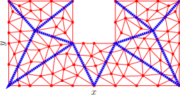
Figure 1. An unstructured mesh with the interface $\Gamma$ (blue-dashed) and cross-points.

This domain decomposition induces a set of non-overlapping triangulations $\{\mathcal{T}_{i}\}_{i=1}^{N_{s}}$. Moreover we can define local DG spaces on each subdomain and represent each function in $V_{h}$ as a direct sum,

$$V_{h}=V_{h,1}\oplus V_{h,2}\oplus\ldots\oplus V_{h,N_{s}},$$

where $V_{h,i}$ for $i=1,\ldots,N_{s}$ is a local space defined as

$$V_{h,i}:=\big{\{}v\in\textrm{L}^{2}(\Omega_{i}):v|_{K\in\mathcal{T}_{i}}\in\mathbb{P}^{k}(K)\big{\}}.$$

We also need a finite dimensional space on the interface which we denote by $\Lambda_{h}$,

$$\Lambda_{h}:=\big{\{}\varphi\in\textrm{L}^{2}(\Gamma):\left.\varphi\right|_{e\in\Gamma}\in\mathbb{P}^{k}(e)\big{\}}.$$

For the analysis of our Schwarz methods we also need to define local spaces on $\Gamma_{i}$ for all $i=1,...,N_{s}$,

$$\Lambda_{i}:=\big{\{}\varphi\in\textrm{L}^{2}(\Gamma_{i}):\left.\varphi\right|_{e\in\Gamma_{i}}\in\mathbb{P}^{k}(e)\big{\}},$$

and its global counterpart $\prod_{i=1}^{N_{s}}\Lambda_{i}$. Note that $\Lambda_{h}$ is single-valued across $\Gamma$ while $\prod_{i=1}^{N_{s}}\Lambda_{i}$ is double-valued. We denote the maximum diameter of the subdomains by $H$ and the diameter of the mono-domain $\Omega$ by $H_{\Omega}$. We assume $0<h\leq H<H_{\Omega}$. For convenience we define a function for the set of neighboring subdomains of $\Omega_{i}$ and denote it by $N(i)$.

2.3. Hybridizable formulation

We now present IPH in a hybridizable form. A DG method is hybridizable if one can eliminate the degrees of freedom inside each element and obtain a linear system in terms of a single-valued function along edges. Not all DG methods can be written in a hybridized form, for instance the classical IP method is not hybridizable. A hybridization procedure for DG methods has been developed and studied in [6] where IPH is also included.

In a DG context the continuity of the exact solution is imposed weakly through a Nitsche penalization technique. Penalization is regulated through a parameter, $\mu\in\textrm{T}(\mathcal{E})$ and scaled like $\mu=\alpha k^{2}/h$ for $\alpha>0$, independent of $h$ and $k$ and sufficiently large. This choice of $\mu$ guarantees coercivity of the DG bilinear form and optimal approximation. Let $(u,\lambda),(v,\varphi)\in V_{h}\times\Lambda_{h}$ and $u_{i},v_{i}\in V_{h,i}$ be the restriction of $u$ and $v$ to $\Omega_{i}$. Then the IPH bilinear form reads

(2.2) $$a((u,\lambda),(v,\varphi)):=a_{\Gamma}(\lambda,\varphi)+\sum_{i=1}^{N_{s}}\Big{(}a_{i}(u_{i},v_{i})+a_{i\Gamma}(v_{i},\lambda)+a_{i\Gamma}(u_{i},\varphi)\Big{)},$$

where

(2.3) $$a_{\Gamma}(\lambda,\varphi):=\mu\sum_{i=1}^{N_{s}}\int_{\Gamma_{i}}\lambda\,\varphi,\quad{a}_{i\Gamma}(v_{i},\varphi):=\int_{\Gamma_{i}}\Big{(}\frac{\partial{v_{i}}}{\partial{{\boldsymbol{n}}_{i}}}-\mu v_{i}\Big{)}\varphi,$$

and the local solvers $a_{i}(\cdot,\cdot)$ are defined as

(2.4) $$\begin{array}[]{rcl}a_{i}(u_{i},v_{i})&:=&\displaystyle\int_{\mathcal{T}_{i}}\eta\,u_{i}\,v_{i}+\nabla u_{i}\cdot\nabla v_{i}-\int_{\mathcal{E}_{i}^{0}}\{\!\!\{\nabla u_{i}\}\!\!\}\cdot[\![v_{i}]\!]+\{\!\!\{\nabla v_{i}\}\!\!\}\cdot[\![u_{i}]\!]\\ &&\displaystyle+\int_{\mathcal{E}^{0}_{i}}\frac{\mu}{2}[\![u_{i}]\!]\cdot[\![v_{i}]\!]-\frac{1}{2\mu}[\![\nabla u_{i}]\!][\![\nabla v_{i}]\!]\displaystyle+\int_{\partial\Omega_{i}}\mu\,u_{i}\,v_{i}-\frac{\partial{u_{i}}}{\partial{{\boldsymbol{n}}_{i}}}v_{i}-\frac{\partial{v_{i}}}{\partial{{\boldsymbol{n}}_{i}}}u_{i}.\end{array}$$

This is an IPH discretization of the model problem in $\Omega_{i}$, and $\partial\Omega_{i}$ is treated as a Dirichlet boundary. Observe that $a_{i}(\cdot,\cdot)$ and $a_{\Gamma}(\cdot,\cdot)$ are symmetric and therefore $a(\cdot,\cdot)$ is symmetric too.

The global bilinear form $a(\cdot,\cdot)$ is coercive at the discrete level. In order to show coercivity we first introduce a semi-norm on each subdomain for all $(v_{i},\varphi)\in V_{h,i}\times\Lambda_{h}$,

(2.5) $$\|{(v_{i},\varphi)}\|_{i}^{2}:=\eta{\|v_{i}\|}_{\mathcal{T}_{i}}^{2}+{\|\nabla v_{i}\|}_{\mathcal{T}_{i}}^{2}+\mu{\|[\![v_{i}]\!]\|}_{\mathcal{E}_{i}\setminus\Gamma_{i}}^{2}+\mu{\|v_{i}-\varphi\|}_{\Gamma_{i}}^{2},$$

for $i=1,..,N_{s}$. Note that if a subdomain is floating, that is it does not touch the Dirichlet boundary condition, and $\eta=0$, then $\|{(v_{i},\varphi)}\|_{i}=0$ implies $v_{i}$ and $\varphi$ are constants and not necessarily zero. The energy norm over the whole domain is defined by

(2.6) $$\|{(v,\varphi)}\|^{2}:=\sum_{i=1}^{N_{s}}\|{(v_{i},\varphi)}\|_{i}^{2}.$$

In order to verify that this is actually a norm, we just need to check its kernel: if $\|{(v,\varphi)}\|=0$ then $v$ and $\varphi$ are both constants and $v|_{\Gamma}=\varphi$. Moreover there are subdomains that touch the Dirichlet boundary condition and therefore $v|_{\partial\Omega}=0$. Hence $(v,\varphi)=0$.

The proof of coercivity for IPH is done subdomain by subdomain: we first collect the contribution of each subdomain

(2.7) $$\begin{array}[]{rcl}{a}((v,\varphi),(v,\varphi))&=&{a}_{\Gamma}(\varphi,\varphi)+\sum_{i=1}^{N_{s}}\big{(}{a}_{i}(v_{i},v_{i})+2{a}_{i\Gamma}(v_{i},\varphi)\big{)},\\ &=&\sum_{i=1}^{N_{s}}\big{(}{a}_{i}(v_{i},v_{i})+2{a}_{i\Gamma}(v_{i},\varphi)+\mu{\|\varphi\|}_{\Gamma_{i}}^{2}\big{)}.\end{array}$$

Each right-hand side can be bounded from below by semi-norms $\|{(v_{i},\varphi)}\|_{i}$ for $i=1,..,N_{s}$; for details see [11, 18]. Then we obtain

$${a}((v,\varphi),(v,\varphi))\geq c\sum_{i=1}^{N_{s}}\|{(v_{i},\varphi)}\|_{i}^{2}=c\|{(v,\varphi)}\|^{2},\quad\forall(v,\varphi)\in V_{h}\times\Lambda_{h},$$

where $0<c<1$ and $c$ does not depend on $h$ and $k$.

An IPH approximation of the exact solution is obtained by solving the following problem: find $(u_{h},\lambda_{h})\in V_{h}\times\Lambda_{h}$ such that

(2.8) $$a((u_{h},\lambda_{h}),(v,\varphi))=\int_{\Omega}f\,v,\quad\forall(v,\varphi)\in V_{h}\times\Lambda_{h},$$

which has a unique solution since $a(\cdot,\cdot)$ is coercive on $V_{h}\times\Lambda_{h}$. We can also show that IPH has optimal approximation properties, i.e., if the weak solution $u$ is regular enough then

$${\|u_{h}-u\|}_{0}\leq c\,h^{k+1}|u|_{k+1,\Omega},$$

see details in [2, 18].

We now describe how subdomains in the discrete problem (2.8) communicate. If we test (2.8) with $\varphi=0$ and $v=0$ in all subdomains except $\Omega_{i}$ we obtain

(2.9) $$a_{i}(u_{i},v_{i})+a_{i\Gamma}(v_{i},\lambda_{h})=\int_{\Omega_{i}}f\,v_{i},\quad\forall v_{i}\in V_{h,i},\text{ for }i=1,\ldots,N_{s},$$

where $u_{i}:=u_{h}|_{\Omega_{i}}$. This shows that $u_{i}$ is determined if $\lambda_{h}$ is known. More precisely $\lambda_{h}$ is used as a Dirichlet boundary data on $\partial\Omega_{i}$ in a weak sense using a Nitsche penalization technique. Now if we test (2.8) with $v=0$ and $\varphi\not=0$, we obtain an equation for $\lambda_{h}$:

(2.10) $$a_{\Gamma}(\lambda_{h},\varphi)+\sum_{i=1}^{N_{s}}a_{i\Gamma}(u_{i},\varphi)=0,\quad\forall\varphi\in\Lambda_{h}.$$

If we further let $\varphi$ be non-zero only on $\Gamma_{ij}$, a segment shared by $\Omega_{i}$ and $\Omega_{j}$, then (2.10) reads

(2.11) $$\lambda_{h}=\frac{1}{2\mu}\Big{(}\mu u_{i}-\frac{\partial{u_{i}}}{\partial{{\boldsymbol{n}}_{i}}}\Big{)}+\frac{1}{2\mu}\Big{(}\mu u_{j}-\frac{\partial{u_{j}}}{\partial{{\boldsymbol{n}}_{j}}}\Big{)},\quad\text{on}\,\Gamma_{ij}.$$

In the language of HDG methods, equation (2.11) is called continuity condition. The continuity condition (2.11) is the core of the optimized Schwarz method that we will describe in Section 3. We have shown in [11] for the case of two subdomains how to exploit (2.11) to design a fast solver which we extend to many subdomains in this paper.

2.4. Schur complement and matrix formulation

The discrete problem (2.8) can be written in an equivalent matrix form. We first choose nodal basis functions for $\mathbb{P}^{k}(K)$ and denote the space of degrees of freedoms (DOFs) of $V_{h}$ by $V$ and similarly for subspaces, denoted by $\{V_{i}\}$. Then the discrete problem (2.8) is equivalent to

(2.12) $$\underbrace{\left[\begin{array}[]{cc}{A_{I}}&{A_{I\Gamma}}\\ {A_{I\Gamma}^{\top}}&{A_{\Gamma}}\end{array}\right]}_{A:=}\left(\begin{array}[]{c}{{\boldsymbol{u}}}\\ {{\boldsymbol{\lambda}}}\end{array}\right)=\left(\begin{array}[]{c}{{\boldsymbol{f}}}\\ {0}\end{array}\right),$$

where ${\boldsymbol{u}}$ and ${\boldsymbol{\lambda}}$ are DOFs corresponding to $u_{h}$ and $\lambda_{h}$, respectively. Here $A_{I}$ corresponds to the bilinear form $\sum_{i=1}^{N_{s}}a_{i}(\cdot,\cdot)$, $A_{I\Gamma}$ corresponds to $\sum_{i=1}^{N_{s}}a_{i\Gamma}(\cdot,\cdot)$ and $A_{\Gamma}$ corresponds to $a_{\Gamma}(\cdot,\cdot)$.

Since the bilinear form (2.2) is symmetric and positive definite we can conclude that $A$ is s.p.d. Hence its diagonal blocks, $A_{I}$ and $A_{\Gamma}$, are also s.p.d. If we eliminate the interface unknown, ${\boldsymbol{\lambda}}$, we arrive at a linear system in terms of primal variables ${\boldsymbol{u}}$ only. This coincides with the primal formulation of IPH, see [11, 18] for details. On the other hand we can eliminate ${\boldsymbol{u}}$ and obtain a Schur complement formulation

(2.13) $$S_{\Gamma}{\boldsymbol{\lambda}}={\boldsymbol{g}},$$

where

(2.14) $$S_{\Gamma}:=A_{\Gamma}-A_{I\Gamma}^{\top}A_{I}^{-1}A_{I\Gamma},\quad{\boldsymbol{g}}:=-A_{I\Gamma}^{\top}A_{I}^{-1}{\boldsymbol{f}}.$$

The Schur complement matrix has smaller dimension compared to (2.12) and is also s.p.d. Therefore one approach in solving (2.13) is to use the conjugate gradient (CG) method. However the convergence of CG is affected by the condition number of $S_{\Gamma}$, which is similar to the condition number of classical FEM Schur complement systems:

Proposition 1.

Let $S_{\Gamma}$ be the Schur complement of the IPH discretization. Then for all $\varphi\in\Lambda_{h}$ we have

(2.15) $$c\frac{H}{H_{\Omega}^{2}}{\|\varphi\|}_{\Gamma}^{2}\leq{\boldsymbol{\varphi}}^{\top}{S}_{\Gamma}{\boldsymbol{\varphi}}\leq C\alpha\frac{k^{2}}{h}{\|\varphi\|}_{\Gamma}^{2},$$

and therefore the condition number $\kappa(S_{\Gamma})$ is bounded by

(2.16) $$\kappa(S_{\Gamma})\leq C\,\alpha\,\frac{H_{\Omega}^{2}k^{2}}{Hh}\kappa(M_{\Gamma}),$$

where $M_{\Gamma}$ is the mass matrix along the interface. Moreover all constants are independent of $\alpha$, $k$, $h$ and $H$.

Proof.

See [17, Appendix 3]. ∎

3. Optimized Schwarz method for IPH

In this section we define and analyze an optimized Schwarz method (OSM) for IPH discretizations. Since an IPH discretization is s.p.d. we can use an additive Schwarz preconditioner in conjunction with CG. However it was first observed in [10] that the convergence mechanism of the additive Schwarz method for IPH is different from classical FEM. For a FEM discretization, the overlap between subdomains makes the additive Schwarz method converge, while for IPH convergence is due to a Robin transmission condition in a non-overlapping setting, and the Robin parameter is exactly the penalty parameter of IPH, $\mu=\alpha\,k^{2}/h$.

Robin transmission conditions are the core of OSM to obtain faster convergence compared to the additive Schwarz method. It was shown in [9] that OSM’s best performance is achieved if the Robin parameter is scaled like $1/\sqrt{h}$. This however poses a contradiction with the IPH discretization penalty parameter since the scaling of $\mu$ cannot be weakened otherwise coercivity and optimal approximation properties are lost. In [11], the authors modified and analyzed an OSM while not changing the scaling of $\mu$. They showed that for the two subdomain case the OSM’s contraction factor is $\rho\leq 1-O(\sqrt{h})$. This is a superior convergence factor compared to additive Schwarz with $\rho\leq 1-O(h)$. If OSM is used as preconditioner for a Krylov subspace method, then a contraction factor of $\rho\leq 1-O(h^{1/4})$ is observed.

We will now define a many subdomain OSM for IPH with this property and then analyze the solver and optimize the performance with respect to the mesh parameter $h$ and the polynomial degree $k$.

3.1. Definition of OSM

We now construct an OSM for the IPH discretization. Observe that from (2.9), we can conclude that $u_{i}\in V_{h,i}$ is determined provided $\lambda_{h}$ is known. Recall also from (2.11) that two subdomains, say $\Omega_{i}$ and $\Omega_{j}$ for $i\not=j$, are communicating using

$$\lambda_{h}=\frac{1}{2\mu}\Big{(}\mu u_{i}-\frac{\partial{u_{i}}}{\partial{{\boldsymbol{n}}_{i}}}\Big{)}+\frac{1}{2\mu}\Big{(}\mu u_{j}-\frac{\partial{u_{j}}}{\partial{{\boldsymbol{n}}_{j}}}\Big{)},\quad\text{on}\,\Gamma_{ij}.$$

Let us now assume that $\lambda_{h}$ is double-valued across the interface $\Gamma$. Then we can assign an interface unknown to each subdomain which we call $\lambda_{i}$ for $i=1,\ldots,N_{s}$, as illustrated in Figure 2.

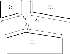
Figure 2. A many subdomain configuration with unknown duplication along interfaces.

Therefore on each interface between two subdomains, say $\Gamma_{ij}$, we should introduce two conditions. We do so by splitting the continuity condition in the following fashion:

(3.1) $$\begin{array}[]{rcr c l}\gamma\lambda_{i}&+&(1-\gamma)\lambda_{j}&=&\frac{1}{2\mu}\Big{(}\mu u_{i}-\frac{\partial{u_{i}}}{\partial{{\boldsymbol{n}}_{i}}}\Big{)}+\frac{1}{2\mu}\Big{(}\mu u_{j}-\frac{\partial{u_{j}}}{\partial{{\boldsymbol{n}}_{j}}}\Big{)},\\ (1-\gamma)\lambda_{i}&+&\gamma\lambda_{j}&=&\frac{1}{2\mu}\Big{(}\mu u_{i}-\frac{\partial{u_{i}}}{\partial{{\boldsymbol{n}}_{i}}}\Big{)}+\frac{1}{2\mu}\Big{(}\mu u_{j}-\frac{\partial{u_{j}}}{\partial{{\boldsymbol{n}}_{j}}}\Big{)},\end{array}$$

where $\gamma\in\mathbb{R}^{+}$ is a “suitable” parameter that we will use to optimize the iterative method. Observe that if we subtract the two conditions in (3.1), we arrive at $(1-2\gamma)(\lambda_{i}-\lambda_{j})=0$. If $\gamma\not=\frac{1}{2}$ then we have $\lambda_{i}=\lambda_{j}=\lambda_{h}$ on all $\Gamma_{ij}$, i.e., we recover the single-valued $\lambda_{h}$ and therefore the solution to the augmented system coincides with the original IPH approximation.

The conditions in (3.1) can be written in an equivalent variational form by multiplying them with appropriate test functions with support on $\partial\Omega_{i}\setminus\partial\Omega$. The advantage is that we can then use the original blocks of the IPH linear system. For a subdomain, e.g., $\Omega_{i}$, we obtain

(3.2) $$\gamma\,a_{\Gamma}^{(i)}(\lambda_{i},\varphi_{i})+a_{i\Gamma}(u_{i},\varphi_{i})+\sum_{j\in N(i)}2\mu(1-\gamma)\int_{\Gamma_{ij}}\lambda_{j}\varphi_{i}+\int_{\Gamma_{ij}}\Big{(}\frac{\partial{u_{j}}}{\partial{{\boldsymbol{n}}_{j}}}-\mu u_{j}\Big{)}\varphi_{i}=0.$$

In order to clarify the definition of the new linear system we provide an example in the case of two subdomains.

Example 3.1 (two subdomain case).

Suppose we have two subdomains and we call the interface between them $\Gamma$. Then an IPH discretization with this configuration looks like

(3.3) $$\left[\begin{array}[]{ccc}{A_{1}}&{}\hfil&{A_{1\Gamma}}\\ {}\hfil&{A_{2}}&{A_{2\Gamma}}\\ {A_{1\Gamma}^{\top}}&{A_{2\Gamma}^{\top}}&{A_{\Gamma}}\end{array}\right]\left(\begin{array}[]{c}{{\boldsymbol{u}}_{1}}\\ {{\boldsymbol{u}}_{2}}\\ {{\boldsymbol{\lambda}}}\end{array}\right)=\left(\begin{array}[]{c}{{\boldsymbol{f}}_{1}}\\ {{\boldsymbol{f}}_{2}}\\ {0}\end{array}\right).$$

Observe that continuity between the two subdomains is imposed through the last row of (3.3). We now suppose ${\boldsymbol{\lambda}}$ is double-valued across the interface, ${\boldsymbol{\lambda}}_{1},{\boldsymbol{\lambda}}_{2}$. Then we introduce two conditions for the two interface unknowns, ${\boldsymbol{\lambda}}_{1}$ and ${\boldsymbol{\lambda}}_{2}$,

$$\begin{array}[]{rcrcccccc}\gamma A_{\Gamma}{\boldsymbol{\lambda}}_{1}&+&(1-\gamma)A_{\Gamma}{\boldsymbol{\lambda}}_{2}&+&A_{1\Gamma}^{\top}{\boldsymbol{u}}_{1}&+&A_{2\Gamma}^{\top}{\boldsymbol{u}}_{2}&=&0,\\ (1-\gamma)A_{\Gamma}{\boldsymbol{\lambda}}_{1}&+&\gamma A_{\Gamma}{\boldsymbol{\lambda}}_{2}&+&A_{1\Gamma}^{\top}{\boldsymbol{u}}_{1}&+&A_{2\Gamma}^{\top}{\boldsymbol{u}}_{2}&=&0,\end{array}$$

where $\gamma\not=\frac{1}{2}$. If we regroup the unknowns according to the subdomain enumeration, then the “augmented” linear system looks like

(3.4) $$\left[\begin{array}[]{cc|cc}A_{1}&A_{1\Gamma}&&\\ A_{1\Gamma}^{\top}&\gamma A_{\Gamma}&A_{2\Gamma}^{\top}&(1-\gamma)A_{\Gamma}\\ \hline\cr&&A_{2}&A_{2\Gamma}\\ A_{1\Gamma}^{\top}&(1-\gamma)A_{\Gamma}&A_{2\Gamma}^{\top}&\gamma A_{\Gamma}\end{array}\right]\left(\begin{array}[]{c}{\boldsymbol{v}}_{1}\\ {\boldsymbol{\lambda}}_{1}\\ {\boldsymbol{v}}_{2}\\ {\boldsymbol{\lambda}}_{2}\end{array}\right)=\left(\begin{array}[]{c}{\boldsymbol{f}}_{1}\\ 0\\ {\boldsymbol{f}}_{2}\\ 0\end{array}\right).$$

Note that provided $\gamma\not=\frac{1}{2}$, the linear systems (3.3) and (3.4) are equivalent in the sense that ${\boldsymbol{v}}_{1}={\boldsymbol{u}}_{1}$ and ${\boldsymbol{u}}_{2}={\boldsymbol{v}}_{2}$ and ${\boldsymbol{\lambda}}_{1}={\boldsymbol{\lambda}}_{2}={\boldsymbol{\lambda}}$.

The authors showed in [11] that for the convergence analysis of a block Jacobi method applied to (3.4) we need to obtain sharp bounds on the eigenvalues of $A_{\Gamma}^{-1}B_{i}$ where

(3.5) $$B_{i}:=A_{i\Gamma}^{\top}A_{i}^{-1}A_{i\Gamma},\quad i=1,2.$$

Such bounds were obtained in [11, Lemma 3.7]. We will further improve the eigenvalue bounds and also obtain sharp estimates with respect to the time step $\tau$, $\eta=\tau^{-1}$.

We are now in the position to define the OSM for an IPH discretization. Formally we first construct the augmented system with double-valued interface unknowns along the interfaces, i.e., (3.4). Then we rearrange the unknowns subdomain by subdomain, i.e., collect $\{({\boldsymbol{u}}_{i},{\boldsymbol{\lambda}}_{i})\}_{i=1}^{N_{s}}$ and finally we perform a block Jacobi method on the augmented linear system with a suitable optimization parameter $\gamma$.

Algorithm 3.2.

Let $\big{\{}(u_{i}^{(0)},\lambda_{i}^{(0)})\big{\}}_{i=1}^{N_{s}}$ be a set of initial guesses for all subdomains. Then for $n=1,2,\ldots$ find $\big{\{}(u_{i}^{(n)},\lambda_{i}^{(n)})\big{\}}_{i=1}^{N_{s}}$ such that

(3.6) $${a}_{i}(u_{i}^{(n)},v_{i})+{a}_{i\Gamma}(v_{i},\lambda_{i}^{(n)})=\int_{\Omega_{i}}f\,v_{i},\quad\forall v_{i}\in V_{h,i},$$

and the continuity condition on $\Gamma_{ij}$ reads

(3.7) $$\gamma\lambda_{i}^{(n)}-\frac{1}{2\mu}\Big{(}\mu u_{i}-\frac{\partial{u_{i}}}{\partial{{\boldsymbol{n}}_{i}}}\Big{)}^{(n)}=-(1-\gamma)\lambda_{j}^{(n-1)}+\frac{1}{2\mu}\Big{(}\mu u_{j}-\frac{\partial{u_{j}}}{\partial{{\boldsymbol{n}}_{j}}}\Big{)}^{(n-1)}.$$

Since the solution of the augmented system coincides with the original IPH linear system, we can conclude that Algorithm 3.2 has the same fixed point as the solution of the IPH discretization.

We call $u_{i}^{(n)}$ satisfying (3.6) with $f=0$ a discrete harmonic extension of $\lambda_{i}$ in $\Omega_{i}$. This definition helps us in analyzing OSM.

Definition 3.3 (Discrete harmonic extension).

For all $\varphi_{i}\in\Lambda_{i}$, we denote by $\mathcal{H}_{i}(\varphi_{i})\in V_{h,i}$ the discrete harmonic extension into $\Omega_{i}$,

(3.8) $$\mathcal{H}_{i}(\varphi)\equiv-A_{i}^{-1}A_{i\Gamma}{\boldsymbol{\varphi}}_{i},$$

where $A_{i}$ and $A_{i\Gamma}$ correspond to the bilinear forms $a_{i}(\cdot,\cdot)$ and $a_{i\Gamma}(\cdot,\cdot)$. The corresponding $\varphi_{i}$ is called generator. In other words $u_{i}:=\mathcal{H}_{i}(\varphi_{i})$ is an approximation obtained from the IPH discretization in $\Omega_{i}$ using $\varphi_{i}$ as Dirichlet data, i.e., $A_{i}{\boldsymbol{u}}_{i}+A_{i\Gamma}{\boldsymbol{\varphi}}_{i}=0$.

There are some questions to be addressed concerning Algorithm 3.2, e.g.,

1. Is Algorithm 3.2 well-posed?

2. Does Algorithm 3.2 converge? If yes, then can we obtain a contraction factor?

3. How to use the optimization parameter $\gamma$ to improve the contraction factor?

4. How do different choice of $\eta$ affect the algorithm and its scalability?

We will answer these questions now in Section 3.2.

3.2. Analysis of OSM

The main goal of this section is to analyze Algorithm 3.2 and answer the questions regarding its well-posedness and convergence. Our analysis is inspired by a similar result for FEM in [21, 22, 23], and we refer the reader to the original work of Lions in [19] for an analysis at the continuous level. Our analysis is however substantially different since DG methods impose continuity across elements weakly. We will first prove

Theorem 3.4 (Convergence estimate).

Let the optimization parameter satisfy $\frac{1}{2}<\gamma\leq 1$. Then Algorithm 3.2 is well-posed and converges. More precisely the following contraction estimate holds

$${\|\mathcal{R}(\varphi^{(n)})\|}^{2}\leq\rho\,{\|\mathcal{R}(\varphi^{(n-1)})\|}^{2},$$

where ${\|\mathcal{R}(\varphi)\|}^{2}:=\sum_{i=1}^{N_{s}}{\|\mathcal{R}_{i}(\varphi_{i})\|}_{\Gamma_{i}}^{2}$ and $\mathcal{R}_{i}(\varphi_{i}):=\gamma\varphi_{i}-\frac{1}{2\mu}\Big{(}\mu-\frac{\partial{}}{\partial{{\boldsymbol{n}}_{i}}}\Big{)}\mathcal{H}_{i}(\varphi_{i})$. Here the contraction factor, i.e., $\rho$, is

(3.9) $$\rho=1-\min\frac{(2\gamma-1)}{\mu(2\gamma-1)^{2}\,C(H,\eta)+1},$$

where $\mu=\alpha{k^{2}}/{h}$ is the penalization parameter and

$$C(H,\eta):=\left\{\begin{array}[]{ll}H&\text{in the case of no floating subdomains},\\ \frac{1}{H\eta}&\text{in the case of floating subdomains}.\end{array}\right.$$

The choice $\gamma=1$ is a special case. It is shown in [11, 16] that in this case Algorithm 3.2 is equivalent to a non-overlapping additive Schwarz method applied to the primal formulation of IPH. The theory for s.p.d. preconditioners, i.e., the abstract Schwarz framework, shows that the condition number of the one-level additive Schwarz method for IPH is bounded by $k^{2}h^{-1}H^{-1}$. This is equivalent to a contraction factor $\rho\leq 1-O(\frac{hH}{k^{2}})$. More precisely, suppose $A$ is the original system matrix in primal form and $A_{\text{add}}$ is the corresponding additive Schwarz preconditioner (see for instance [24, Section 1.5]) then the block Jacobi method converges with the aforementioned contraction factor in the $A$-norm. It is easy to see that our analysis also reveals the same contraction factor (in the ${\|\mathcal{R}(\cdot)\|}$ norm) in this special case: let $\gamma=1$ in (3.9) and recall that $\mu=\alpha{k^{2}}/{h}$. Then, we have

(3.10) $$\rho\leq 1-O\Big{(}\frac{hH}{k^{2}}\Big{)},$$

as $h$ and $H$ go to zero or $k$ goes to infinity.

Our second objective of this section is to minimize the contraction factor through a suitable choice of the optimization parameter $\gamma$. This is stated in

Corollary 3.5 (Optimized contraction factor).

Let $\eta=\tau^{-1}$ where $\tau$ is the time-step which is chosen to be $O(1)$ or $O(H)$ or $O(H^{2})$. Then the optimized contraction factor for Algorithm 3.2 for the different choices of $\tau$ is

(3.11) $$\rho_{\text{opt}}\leq\left\{\begin{array}[]{lll}1-O(\frac{\sqrt{hH}}{k})&\text{for }\tau=O(1),&\text{if }\gamma_{\text{opt}}=\frac{1}{2}(1+\frac{\sqrt{hH}}{k}),\\ 1-O(\frac{\sqrt{h}}{k})&\text{for }\tau=O(H),&\text{if }\gamma_{\text{opt}}=\frac{1}{2}(1+\frac{\sqrt{h}}{k}),\\ 1-O(\sqrt{\frac{h}{H}}\frac{1}{k})&\text{for }\tau=O(H^{2}),&\text{if }\gamma_{\text{opt}}=\frac{1}{2}(1+\sqrt{\frac{h}{H}}\frac{1}{k}).\end{array}\right.$$

Observe that the $h$-dependency and $k$-dependency is weakened by a square-root compared to (3.10). Moreover if the time-step is chosen to scale like a forward Euler time-step, i.e., $O(H^{2})$, then Algorithm 3.2 is scalable.

Proof of Theorem 3.4. We first show that Algorithm 3.2 is well-posed, i.e., we can actually iterate. By linearity we assume that $f=0$. We proceed by eliminating $u_{i}^{(n)}$ for all subdomains and simplify Algorithm 3.2 to: for all subdomains, find $\lambda_{i}^{(n)}$ such that

(3.12) $$\gamma\lambda_{i}^{(n)}-\frac{1}{2\mu}\Big{(}\mu-\frac{\partial{}}{\partial{{\boldsymbol{n}}_{i}}}\Big{)}\mathcal{H}_{i}(\lambda_{i}^{(n)})=-(1-\gamma)\lambda_{j}^{(n-1)}+\frac{1}{2\mu}\Big{(}\mu-\frac{\partial{}}{\partial{{\boldsymbol{n}}_{j}}}\Big{)}\mathcal{H}_{j}(\lambda_{j}^{(n-1)}),$$

on $\Gamma_{ij}$ for all $j\in N(i)$, where $N(i)$ is the set of neighboring subdomains of $\Omega_{i}$. Let us denote the linear operator on the left-hand side by $\mathcal{R}_{i}:\Lambda_{i}\rightarrow\Lambda_{i}$, that is

(3.13) $$\mathcal{R}_{i}(\varphi_{i}):=\gamma\varphi_{i}-\frac{1}{2\mu}\Big{(}\mu-\frac{\partial{}}{\partial{{\boldsymbol{n}}_{i}}}\Big{)}\mathcal{H}_{i}(\varphi_{i}).$$

If we show that $\mathcal{R}_{i}(\cdot)$ is an invertible operator, then Algorithm 3.2 is well-posed. We show $\mathcal{R}_{i}(\cdot)$ is invertible by showing that it is injective:

Lemma 3.6.

If $\gamma>\frac{1}{2}$ then the operator $\mathcal{R}_{i}(\cdot)$ is injective for all $i=1,\ldots,N_{s}$. More precisely we have the estimate

(3.14) $${\|\mathcal{R}_{i}(\varphi_{i})\|}_{\Gamma_{i}}\geq\Big{(}\gamma-\frac{1}{2}+c(h,H,k)\Big{)}{\|\varphi_{i}\|}_{\Gamma_{i}},\quad\forall\varphi_{i}\in\Lambda_{i},$$

where

$$c(h,H,k):=\left\{\begin{array}[]{ll}c\frac{h}{H}\frac{1}{k^{2}}&\text{for non-floating subdomains},\\ 0&\text{for floating subdomains}.\end{array}\right.$$

Proof.

We multiply $\mathcal{R}_{i}(\varphi_{i})$ by $\varphi_{i}$ and integrate over $\Gamma_{i}$,

$$\int_{\Gamma_{i}}\mathcal{R}_{i}(\varphi_{i})\,\varphi_{i}=\gamma{\|\varphi_{i}\|}_{\Gamma_{i}}^{2}+\frac{1}{2\mu}a_{i\Gamma}(u_{i},\varphi_{i}),$$

where $u_{i}:=\mathcal{H}_{i}(\varphi_{i})$. Recall that if $u_{i}$ is the harmonic extension of $\varphi_{i}$ then $a_{i}(u_{i},u_{i})+a_{i\Gamma}(u_{i},\varphi_{i})=0$. Therefore we have $\int_{\Gamma_{i}}\mathcal{R}_{i}(\varphi_{i})\,\varphi_{i}=\gamma{\|\varphi_{i}\|}_{\Gamma_{i}}^{2}-\frac{1}{2\mu}a_{i}(u_{i},u_{i}).$ We can show that $a(u_{i},u_{i})\leq\big{(}1-c(h,H,k)\big{)}\mu{\|\varphi_{i}\|}_{\Gamma_{i}}^{2}$, see Appendix A, and obtain

$$\int_{\Gamma_{i}}\mathcal{R}_{i}(\varphi_{i})\,\varphi_{i}\geq\big{(}\gamma-\frac{1}{2}+c(h,H,k)\big{)}{\|\varphi_{i}\|}_{\Gamma_{i}}^{2}.$$

If $\gamma>\frac{1}{2}$, then the right-hand side is positive. Now we apply the Cauchy-Schwarz inequality to the left-hand side and obtain ${\|\mathcal{R}_{i}(\varphi_{i})\|}_{\Gamma_{i}}\geq\big{(}\gamma-\frac{1}{2}+c(h,H,k)\big{)}{\|\varphi_{i}\|}_{\Gamma_{i}}$ which completes the proof. ∎

Note that Lemma 3.6 provides a lower bound for the norm-equivalence between ${\|\mathcal{R}_{i}(\cdot)\|}_{\Gamma_{i}}$ and the $\textrm{L}^{2}$-norm, i.e., ${\|\cdot\|}_{\Gamma_{i}}$. The upper bound in the norm-equivalence can be also obtained, as we show in the following proposition.

Proposition 2 (Norm equivalence).

The two norms ${\|\mathcal{R}_{i}(\cdot)\|}_{\Gamma_{i}}$ and ${\|\cdot\|}_{\Gamma_{i}}$ are equivalent,

$$C{\|\varphi_{i}\|}_{\Gamma_{i}}\geq{\|\mathcal{R}_{i}(\varphi_{i})\|}_{\Gamma_{i}}\geq\Big{(}\gamma-\frac{1}{2}+c(h,H,k)\Big{)}{\|\varphi_{i}\|}_{\Gamma_{i}},\quad\forall\varphi_{i}\in\Lambda_{i},$$

where $C>0$ is independent of $h,H,\alpha$ and $\eta$. Here $c(h,H,k)$ is the constant defined in Lemma 3.6.

Proof.

The lower bound estimate is from Lemma 3.6. For the upper bound we use the estimate from Lemma 3.10 (which will appear in Section 3.3). More precisely we have

$${\boldsymbol{\varphi}}_{i}^{\top}B_{i}{\boldsymbol{\varphi}}_{i}\geq c\mu{\|\mathcal{R}_{i}(\varphi_{i})\|}_{\Gamma_{i}}^{2},$$

where $B_{i}:=A_{i\Gamma}^{\top}A_{i}^{-1}A_{i\Gamma}$ (see Example 3.1). We then use the estimate for the eigenvalues of $B_{i}$, i.e., [11, Lemma 3.7] to obtain

$$\mu{\|\varphi_{i}\|}_{\Gamma_{i}}^{2}\geq{\boldsymbol{\varphi}}_{i}^{\top}B_{i}{\boldsymbol{\varphi}}_{i}\geq c\mu{\|\mathcal{R}_{i}(\varphi_{i})\|}_{\Gamma_{i}}^{2}.$$

This completes the proof. ∎

Since $\mathcal{R}_{i}(\cdot)$ is linear and injective we conclude that it induces a local norm on $\Lambda_{i}$. We can also define a global norm on the space of $\prod_{i=1}^{N_{s}}\Lambda_{i}$ by

(3.15) $${\|\mathcal{R}({\varphi})\|}^{2}:=\sum_{i=1}^{N_{s}}{\|\mathcal{R}_{i}(\varphi_{i})\|}_{\Gamma_{i}}^{2},\quad\forall{\varphi}\in\prod_{i=1}^{N_{s}}\Lambda_{i},$$

where ${\varphi}:=(\varphi_{1},\varphi_{2},\ldots,\varphi_{N_{s}})$. This turns out to be the right norm for the convergence analysis of Algorithm 3.2.

We can now show that Algorithm 3.2 converges with a concrete contraction factor estimate. The right-hand side of the iteration equation (3.12) can be simplified to

(3.16) $$\mathcal{R}_{i}(\varphi_{i}^{(n)})=(2\gamma-1)\varphi_{j}^{(n-1)}-\mathcal{R}_{j}(\varphi_{j}^{(n-1)}),$$

on $\Gamma_{ij}$ for all $j\in N(i)$. Note that $2\gamma-1$ is strictly-positive with our condition $\gamma>\frac{1}{2}$. For a given subdomain, say $\Omega_{i}$, we take the $\textrm{L}^{2}$-norm on both sides. To simplify the presentation, we suppress the iteration index for the moment, but terms on the left-hand side are evaluated at iteration $(n)$ while on the right-hand side they are evaluated at iteration index $(n-1)$:

$$\begin{array}[]{rcl}{\|\mathcal{R}_{i}(\varphi_{i})\|}_{\Gamma_{ij}}^{2}&=&{\|\mathcal{R}_{j}(\varphi_{j})-(2\gamma-1)\varphi_{j}\|}_{\Gamma_{ij}}^{2}\\ &=&{\|\mathcal{R}_{j}(\varphi_{j})\|}_{\Gamma_{ij}}^{2}+{\|(2\gamma-1)\varphi_{j}\|}_{\Gamma_{ij}}^{2}-2(2\gamma-1)\int_{\Gamma_{ij}}\mathcal{R}_{j}(\varphi_{j})\,\varphi_{j}\\ &=&{\|\mathcal{R}_{j}(\varphi_{j})\|}_{\Gamma_{ij}}^{2}+\big{[}(2\gamma-1)^{2}-2(2\gamma-1)\gamma\big{]}{\|\varphi_{j}\|}_{\Gamma_{ij}}^{2}\\ &&\qquad\qquad\quad+\frac{1}{\mu}(2\gamma-1)\int_{\Gamma_{ij}}\big{(}\mu u_{j}-\frac{\partial{u_{j}}}{\partial{{\boldsymbol{n}}_{j}}}\big{)}\varphi_{j}\\ &=&{\|\mathcal{R}_{j}(\varphi_{j})\|}_{\Gamma_{ij}}^{2}-(2\gamma-1)\Big{[}{\|\varphi_{j}\|}_{\Gamma_{ij}}^{2}-\frac{1}{\mu}\int_{\Gamma_{ij}}\big{(}\mu u_{j}-\frac{\partial{u_{j}}}{\partial{{\boldsymbol{n}}_{j}}}\big{)}\varphi_{j}\Big{]}.\end{array}$$

Then we sum over all interfaces of $\Omega_{i}$ and all subdomains to obtain

(3.17) $$\begin{array}[]{rcl}{\|\mathcal{R}(\varphi)\|}^{2}&=&\sum_{i=1}^{N_{s}}\sum_{j\in N(i)}{\|\mathcal{R}_{j}(\varphi_{j})\|}_{\Gamma_{ij}}^{2}\\ &&\qquad\qquad\quad-(2\gamma-1)\mu^{-1}\Big{[}\mu{\|\varphi_{j}\|}_{\Gamma_{ij}}^{2}-\int_{\Gamma_{ij}}\big{(}\mu u_{j}-\frac{\partial{u_{j}}}{\partial{{\boldsymbol{n}}_{j}}}\big{)}\varphi_{j}\Big{]}\\ &=&{\|\mathcal{R}(\varphi)\|}^{2}\\ &&\qquad-(2\gamma-1)\mu^{-1}\sum_{m=1}^{N_{s}}\Big{[}\mu{\|\varphi_{m}\|}_{\Gamma_{m}}^{2}+a_{m\Gamma}(u_{m},\varphi_{m})\Big{]}\\ &=&{\|\mathcal{R}(\varphi)\|}^{2}\\ &&\qquad-(2\gamma-1)\mu^{-1}\sum_{m=1}^{N_{s}}\Big{[}\mu{\|\varphi_{m}\|}_{\Gamma_{m}}^{2}-a_{m}(u_{m},u_{m})\Big{]}\\ &\leq&{\|\mathcal{R}(\varphi)\|}^{2}-c(2\gamma-1)\mu^{-1}\sum_{m=1}^{N_{s}}{\|(u_{m},\varphi_{m})\|}_{m}^{2},\end{array}$$

where for the left-hand side we used

$$\sum_{i=1}^{N_{s}}\sum_{j\in N(i)}{\|\mathcal{R}_{i}(\varphi_{i})\|}_{\Gamma_{ij}}^{2}=\sum_{i=1}^{N_{s}}{\|\mathcal{R}_{i}(\varphi_{i})\|}_{\Gamma_{i}}^{2}=:{\|\mathcal{R}(\varphi)\|}^{2},$$

and for the right-hand side we used the coercivity inequality

$$\mu{\|\varphi_{m}\|}_{\Gamma_{m}}^{2}-a_{m}(u_{m},u_{m})\geq c{\|(u_{m},\varphi_{m})\|}_{m}^{2},$$

see Appendix A for details. Note that ${\|(u_{m},\varphi_{m})\|}_{m}$ is subdomain-wise positive definite if $\eta>0$. More precisely we can show that if $\eta>0$ then for all subdomains, even floating ones, we have the estimate

(3.18) $${\|\mathcal{R}_{m}(\varphi_{m})\|}_{\Gamma_{m}}^{2}\leq\Big{(}(2\gamma-1)^{2}C(H,\eta)+\mu^{-1}\Big{)}{\|(u_{m},\varphi_{m})\|}_{m}^{2},$$

where

(3.19) $$C(H,\eta):=\left\{\begin{array}[]{ll}H&\text{for non-floating subdomain},\\ \frac{1}{H\eta}&\text{for floating subdomain}.\end{array}\right.$$

Note that (3.18) makes sense only if $\eta>0$ since ${\|(\cdot,\cdot)\|}_{m}$ is only a semi-norm for floating subdomains if $\eta=0$ while ${\|\mathcal{R}_{m}(\cdot)\|}_{\Gamma_{m}}$ is a norm, see Appendix A, in particular (A.9) and (A.7). We have ignored the $\eta{\|u_{i}\|}_{\Omega_{i}}$ term in (A.7) for simplicity of the exposition; the $\eta{\|u_{i}\|}_{\Omega_{i}}$ term in (A.7) will be exploited in Section 3.3.

We then insert the norm estimate (3.18) into the last inequality of (3.17) and reintroduce the iteration index to obtain

(3.20) $${\|\mathcal{R}(\varphi^{(n)})\|}^{2}\leq\Big{(}1-\min\Big{\{}\frac{2\gamma-1}{\mu(2\gamma-1)^{2}H+1},\frac{2\gamma-1}{\mu(2\gamma-1)^{2}(H\eta)^{-1}+1}\Big{\}}\Big{)}{\|\mathcal{R}(\varphi^{(n-1)})\|}^{2},$$

which shows convergence and proves Theorem 3.4.

Proof of Corollary 3.5. We need to choose a suitable $\gamma>\frac{1}{2}$ to achieve the best possible contraction factor. In order to weaken dependencies on the mesh parameter, subdomain diameter and polynomial degree, we make for the optimization parameter the ansatz

(3.21) $$\gamma=\frac{1}{2}\Big{(}1+\frac{h^{\xi}H^{\zeta}}{k^{\psi}}\Big{)},$$

with $\xi,\zeta,\psi\in\mathbb{R}$ to be chosen. We would like to minimize the contraction factor, i.e.,

(3.22) $$\rho_{\text{opt}}\leq 1-\max_{\xi,\zeta,\psi}\,\min\Big{\{}\frac{{h^{\xi}H^{\zeta}}}{k^{2-\psi}h^{2\xi-1}H^{2\zeta+1}+k^{\psi}},\frac{{h^{\xi}H^{\zeta}}}{k^{2-\psi}h^{2\xi-1}H^{2\zeta-1}\eta^{-1}+k^{\psi}}\Big{\}}.$$

Remark 3.7 (On the choice of $\gamma$).

It has been shown in [16] and [17, Section 3.2] that the transmission condition between two subdomains in Algorithm 3.2 is equivalent at the continuous level to

$$\Big{(}(2\gamma-1)\mu\,u_{1}+\frac{\partial{u_{1}}}{\partial{{\boldsymbol{n}}_{1}}}\Big{)}^{(n)}=\Big{(}(2\gamma-1)\mu\,u_{2}+\frac{\partial{u_{2}}}{\partial{{\boldsymbol{n}}_{1}}}\Big{)}^{(n-1)}.$$

It has been shown (at the continuous level [9]) that the optimal choice of the Robin parameter is $(2\gamma-1)\mu=O(h^{-1/2})$. This translates to choosing $\gamma=\frac{1}{2}(1+\sqrt{h})$. We will show that this is also the optimal scaling at the discrete level. In [9], it has been shown that the optimal scaling of the Robin parameter is $O((hL)^{-1/2})$ where $L$ is the length of the interface and it can be viewed as a measure of the diameter of a subdomain, i.e., $H$. This motivates our choice of optimization parameter, i.e., $\gamma$.

When dealing with parabolic problems, $\eta={\tau^{-1}}$ and $\tau$ is the time-step. Therefore it is reasonable to optimize $\gamma$ for different choices of the time-step.

• $\tau=O(1)$: we start with the dependence on the polynomial degree. Observe that the weakest dependence is achieved if we let $\psi=1$. This leads to $\rho\leq 1-O(\frac{1}{k})$, which compares very favorably to (3.10). Now we consider the case where $H$ is fixed and we refine the mesh, $h\rightarrow 0$. Then $\xi=\frac{1}{2}$ is the optimal choice which yields $\rho\leq 1-O(\frac{\sqrt{h}}{k})$. This leads to a simplified bound for $\rho_{\text{opt}}$, namely

  $$\rho_{\text{opt}}\leq 1-\max_{\zeta}\,\min\Big{\{}\frac{H^{\zeta}}{H^{2\zeta+1}+1},\frac{H^{\zeta}}{H^{2\zeta-1}+1}\Big{\}}O(\frac{\sqrt{h}}{k}).$$

  The optimal value for $\zeta$ is therefore $\frac{1}{2}$. We thus obtain the optimal parameter and corresponding contraction factor

  (3.23) $$\gamma_{\text{opt}}:=\frac{1}{2}\Big{(}1+\frac{\sqrt{hH}}{k}\Big{)},\quad\rho_{\text{opt}}\leq 1-O\big{(}\frac{\sqrt{hH}}{k}\big{)},\quad\text{if }\tau=O(1).$$

• $\tau=O(H)$: The best parameters with respect to $k$ and $h$ follow the same argument as before. For optimization with respect to $H$ we have now

  $$\rho_{\text{opt}}\leq 1-\max_{\zeta}\,\min\Big{\{}\frac{H^{\zeta}}{H^{2\zeta+1}+1},\frac{H^{\zeta}}{H^{2\zeta}+1}\Big{\}}O(\frac{\sqrt{h}}{k}).$$

  In this case we can eliminate the $H$-dependence by choosing $\zeta=0$. Hence we have

  (3.24) $$\gamma_{\text{opt}}:=\frac{1}{2}\Big{(}1+\frac{\sqrt{h}}{k}\Big{)},\quad\rho_{\text{opt}}\leq 1-O\big{(}\frac{\sqrt{h}}{k}\big{)},\quad\text{if }\tau=O(H).$$

• $\tau=O(H^{2})$: This case is comparable to using a forward Euler method where $\tau$ is required to be proportional to $h^{2}$. This is a typical constraint when dealing with parabolic problems and accurate trajectories in time are needed, but one could still take larger time steps in our setting than with forward Euler due to a larger constant. We proceed as before by choosing the same parameters with respect to $k$ and $h$. For the $H$-dependence we have

  $$\rho_{\text{opt}}\leq 1-\max_{\zeta}\,\min\Big{\{}\frac{H^{\zeta}}{H^{2\zeta+1}+1},\frac{H^{\zeta}}{H^{2\zeta+1}+1}\Big{\}}O(\frac{\sqrt{h}}{k}).$$

  The optimal parameter hence is $\zeta=-\frac{1}{2}$ which yields

  (3.25) $$\gamma_{\text{opt}}:=\frac{1}{2}\Big{(}1+\sqrt{\frac{h}{H}}\frac{1}{k}\Big{)},\quad\rho_{\text{opt}}\leq 1-O\big{(}\sqrt{\frac{h}{H}}\frac{1}{k}\big{)},\quad\text{if }\tau=O(H^{2}).$$

  Note that this choice of $\gamma_{\text{opt}}$ is still feasible since $h\leq H$ and therefore $\gamma_{\text{opt}}\leq 1$. This shows that the method is weakly scalable if we choose a small enough time-step, without the need of a coarse solver. A similar result for the additive Schwarz method and FEM exists, see [4, Theorem 4].

This completes the proof of Corollary 3.5.

3.3. A refined contraction factor with respect to the time-step

In this section we would like to investigate the effect of the time-step, $\tau=\eta^{-1}$, on the contraction factor while the number of subdomains is fixed, e.g., in the case of two subdomains. This has so far not been addressed, neither in [21] nor in the authors’ paper [11] which deals with two subdomains only.

Suppose for the moment that we have two subdomains. Then as mentioned in Example 3.1 and proved in [11] the convergence of the OSM is governed by the eigenvalues of $A_{\Gamma}^{-1}B_{i}$ where $B_{i}:=A_{i\Gamma}^{\top}A_{i}^{-1}A_{i\Gamma}$. We would like to obtain eigenvalue estimates that depend on $\eta$. This is stated in the following lemma which improves the estimate in [11, Lemma 3.7].

Lemma 3.8.

Let $B_{i}:=A_{i\Gamma}^{\top}A_{i}^{-1}A_{i\Gamma}$ for $i=1,2$ where $A_{i}$ and $A_{i\Gamma}$ correspond to the bilinear forms defined in (2.4) and (2.3), respectively. Then for $\eta\geq 0$ we have the estimate

$${\boldsymbol{\varphi}}^{\top}B_{i}{\boldsymbol{\varphi}}\leq\bigg{(}\frac{1}{1+\frac{C\eta\,h^{2}}{1+C\eta\,h^{2}}}\bigg{)}\Big{(}1-{c}\frac{h}{H\alpha}\Big{)}\mu{\|\varphi\|}_{\Gamma}^{2},$$

where $c$ and $C$ are positive constants which are independent of $h,H,\alpha$ and $\eta$.

Proof.

Recall the definition of $A_{i}$ from (2.4), and let us decompose $A_{i}$ into the mass matrix $M_{i}$ and the stiffness matrix $K_{i}$,

$$A_{i}:=\eta M_{i}+K_{i},$$

where ${\boldsymbol{v}}_{i}^{\top}M_{i}{\boldsymbol{u}}_{i}:=\int_{\Omega_{i}}u_{i}\,v_{i}$ and $K_{i}$ is defined as ${\boldsymbol{v}}_{i}^{\top}K_{i}{\boldsymbol{u}}_{i}:=a_{i}(u_{i},v_{i})-\eta\,{\boldsymbol{v}}_{i}^{\top}M_{i}{\boldsymbol{u}}_{i}$. Consider now

$$\hat{A}:=\left[\begin{array}[]{cc}{K_{i}+\eta M_{i}}&{A_{i\Gamma}}\\ {A_{i\Gamma}^{\top}}&{\frac{1}{2}A_{\Gamma}}\end{array}\right],$$

which is coercive, i.e., for all ${\boldsymbol{w}}:=({\boldsymbol{u}}_{i},{\boldsymbol{\varphi}})$ we have (see [11, Equation 3.6]),

(3.26) $${\boldsymbol{w}}^{\top}\hat{A}{\boldsymbol{w}}\geq c\,\|{(u_{i},\varphi)}\|_{i}^{2}\geq\eta\,{\boldsymbol{u}}_{i}^{\top}M_{i}{\boldsymbol{u}}_{i}+\frac{c}{H}{\|\varphi\|}_{\Gamma}^{2},$$

where the last inequality is Lemma A.1. On the other hand we can easily verify that for $u_{i}:=\mathcal{H}_{i}(\varphi)$ we have

(3.27) $${\boldsymbol{\varphi}}^{\top}B_{i}{\boldsymbol{\varphi}}={\boldsymbol{u}}_{i}^{\top}\big{(}K_{i}+\eta M_{i}\big{)}{\boldsymbol{u}}_{i}\leq\big{(}Ch^{-2}+\eta\big{)}{\boldsymbol{u}}_{i}^{\top}M_{i}{\boldsymbol{u}}_{i},$$

where we have used the fact that $\sigma(M_{i}^{-1}K_{i})\in[c_{1},c_{2}\,h^{-2}]$, which is usual for elliptic operators, see for instance [5, Theorem 3.4]. For ${\boldsymbol{w}}:=(\mathcal{H}_{i}(\varphi),\varphi)$, observing that

$$\frac{1}{2}{\boldsymbol{\varphi}}^{\top}A_{\Gamma}{\boldsymbol{\varphi}}-{\boldsymbol{\varphi}}^{\top}B_{i}{\boldsymbol{\varphi}}={\boldsymbol{w}}^{\top}\hat{A}{\boldsymbol{w}},$$

and using (3.26) we have

$$\frac{1}{2}{\boldsymbol{\varphi}}^{\top}A_{\Gamma}{\boldsymbol{\varphi}}-{\boldsymbol{\varphi}}^{\top}B_{i}{\boldsymbol{\varphi}}\geq\frac{\eta}{Ch^{-2}+\eta}{\boldsymbol{\varphi}}^{\top}B_{i}{\boldsymbol{\varphi}}+\frac{c}{H}{\|\varphi\|}_{\Gamma}^{2}.$$

Recalling that $\frac{1}{2}{\boldsymbol{\varphi}}^{\top}A_{\Gamma}{\boldsymbol{\varphi}}=\mu{\|\varphi\|}_{\Gamma}^{2}$ we can conclude

(3.28) $$\bigg{(}\frac{1}{1+\frac{C\eta\,h^{2}}{1+C\eta\,h^{2}}}\bigg{)}\Big{(}1-{c}\frac{h}{H\alpha}\Big{)}\mu{\|\varphi\|}_{\Gamma}^{2}\geq{\boldsymbol{\varphi}}^{\top}B_{i}{\boldsymbol{\varphi}}.$$

This completes the proof. ∎

We can use Lemma 3.8 to obtain a sharper contraction factor for the two subdomain case with respect to $\eta$. In the following corollary, we study the effect of $\eta$ on the contraction factor. We consider only the case when $\gamma=1$ for clarity of the presentation. However it is possible to use a combination of $\gamma$ and the time-step $\tau=\eta^{-1}$ to optimize the contraction factor. Observe that in the following corollary, if $\eta=O(h^{-2})$ then the contraction factor is independent of the mesh-size.

Theorem 3.9.

Consider the two-subdomain case and let $\gamma=1$. Then the error of the interface variable satisfies the contraction estimate

$${\|\mathbf{e}_{i}^{(n)}\|}_{E_{i}^{\top}E_{i}}\leq\rho(h,H,\eta)\,{\|\mathbf{e}_{i}^{(n-1)}\|}_{E_{i}^{\top}E_{i}}\quad\text{for }i=1,2,$$

where $E_{i}:=A_{\Gamma}^{1/2}(1-A_{\Gamma}^{-1}B_{i})$ and

$$\rho(h,H,\eta):=\begin{cases}1-c\frac{h}{H\alpha}&\text{for }\eta=O(1)\text{ and }O(h^{-1}),\\ 1-C&\text{for }\eta=O(h^{-2}).\end{cases}$$

Proof.

The proof relies on the proof given in [11, Section 4.1]. In the case of the two-subdomain case with $\gamma=1$ we have from [11, Section 4.1] that

$${\|\mathbf{e}_{i}^{(n)}\|}_{E_{i}^{\top}E_{i}}\leq\rho(h,H,\eta)\,{\|\mathbf{e}_{i}^{(n-1)}\|}_{E_{i}^{\top}E_{i}}\quad\text{for }i=1,2,$$

where

$$\rho(h,H,\eta):=\left[\bigg{(}\frac{1}{1+\frac{C\eta\,h^{2}}{1+C\eta\,h^{2}}}\bigg{)}\Big{(}1-{c}\frac{h}{H\alpha}\Big{)}\right]^{2},$$

which is the square of the upper bound constant in (3.28) divided by $\mu$. Choosing $\eta=O(1),O(h^{-1})$ and $O(h^{-2})$ completes the proof. In particular, observe that for $\eta=O(h^{-2})$ we have

$$\bigg{(}\frac{1}{1+\frac{C\eta\,h^{2}}{1+C\eta\,h^{2}}}\bigg{)}\Big{(}1-{c}\frac{h}{H\alpha}\Big{)}\leq\Big{(}\frac{1-C_{2}\,h}{1+C_{3}}\Big{)}\leq\Big{(}\frac{1}{1+C_{3}}\Big{)}.$$

This shows that with a time-step of the size of a forward Euler method, the algorithm converges in a fixed number of iterations since $\frac{1}{1+C_{3}}<1$ uniformly in $h$. ∎

Let us now extend the above result to the case of many non-floating subdomains. In order to do so, we first need the following lemma that relates the $\mathcal{R}_{i}(\cdot)$ operator to $B_{i}$.

Lemma 3.10.

Let $B_{i}:=A_{i\Gamma}^{\top}A_{i}^{-1}A_{i\Gamma}$ and $\mathcal{R}_{i}(\varphi_{i}):=\gamma\varphi_{i}-\frac{1}{2\mu}\Big{(}\mu-\frac{\partial{}}{\partial{{\boldsymbol{n}}_{i}}}\Big{)}\mathcal{H}_{i}(\varphi_{i})$ for $\Omega_{i}$ which is a non-floating subdomain. Then the following estimate holds

(3.29) $$c\,\mu\,{\|\mathcal{R}_{i}(\varphi_{i})\|}_{\Gamma_{i}}^{2}\leq{\boldsymbol{\varphi}}_{i}^{\top}B_{i}{\boldsymbol{\varphi}}_{i},$$

where $c$ is independent of $h,\alpha$ and $\eta$. Moreover let $u_{i}=\mathcal{H}_{i}(\varphi_{i})$, then we have

(3.30) $$\Big{(}\frac{\eta}{\eta+C\,h^{-2}}\Big{)}\cdot c\,\mu\,{\|\mathcal{R}_{i}(\varphi_{i})\|}_{\Gamma_{i}}^{2}\leq\eta{\|u_{i}\|}_{\Omega_{i}}^{2}.$$

Proof.

We take the $\textrm{L}^{2}$-norm of $\mathcal{R}_{i}(\varphi_{i})$ and use the triangle and Young’s inequality to obtain

$${\|\mathcal{R}_{i}(\varphi_{i})\|}_{\Gamma_{i}}^{2}\leq 2\gamma^{2}{\|\varphi_{i}\|}_{\Gamma_{i}}^{2}+\frac{1}{2\mu^{2}}{\|z_{i}\|}_{\Gamma_{i}}^{2},$$

where $z_{i}:=(\mu-\partial_{{\boldsymbol{n}}_{i}})u_{i}\in\Lambda_{i}$. We know from [11, Proposition 2.4] that ${\boldsymbol{z}}_{i}=M_{\Gamma_{i}}^{-1}B_{i}{\boldsymbol{\varphi}}_{i}$. Then we have

$${\|z_{i}\|}_{\Gamma_{i}}^{2}={\boldsymbol{\varphi}}_{i}^{\top}B_{i}M_{\Gamma_{i}}^{-1}M_{\Gamma_{i}}M_{\Gamma_{i}}^{-1}B_{i}{\boldsymbol{\varphi}}={\boldsymbol{\varphi}}_{i}^{\top}B_{i}M_{\Gamma_{i}}^{-1}B_{i}{\boldsymbol{\varphi}}_{i}={\boldsymbol{\varphi}}_{i}^{\top}B_{i}^{1/2}(B_{i}^{1/2}M_{\Gamma_{i}}^{-1}B_{i}^{1/2})B_{i}^{1/2}{\boldsymbol{\varphi}}_{i},$$

since $B_{i}$ is s.p.d. A simple calculation shows that $\sigma(B_{i}^{1/2}M_{\Gamma_{i}}^{-1}B_{i}^{1/2})=\sigma(M_{\Gamma_{i}}^{-1}B_{i})$. Recall that $A_{\Gamma_{i}}=2\mu M_{\Gamma_{i}}$. Then for $z_{i}$ we have from the eigenvalues of $A_{\Gamma_{i}}^{-1}B_{i}$, see [11, Equation 3.1],

$${\|z_{i}\|}_{\Gamma_{i}}^{2}\leq{2\mu}\cdot\sigma_{\max}(A_{\Gamma_{i}}^{-1}B_{i})\cdot{\boldsymbol{\varphi}}_{i}^{\top}B_{i}{\boldsymbol{\varphi}}_{i}\leq 2\mu\cdot{\boldsymbol{\varphi}}_{i}^{\top}B_{i}{\boldsymbol{\varphi}}_{i}.$$

This yields

$${\|\mathcal{R}_{i}(\varphi_{i})\|}_{\Gamma_{i}}^{2}\leq 2\gamma^{2}{\|\varphi_{i}\|}_{\Gamma_{i}}^{2}+\mu^{-1}{\boldsymbol{\varphi}}_{i}^{\top}B_{i}{\boldsymbol{\varphi}}_{i}\leq 2{\|\varphi_{i}\|}_{\Gamma_{i}}^{2}+\mu^{-1}{\boldsymbol{\varphi}}_{i}^{\top}B_{i}{\boldsymbol{\varphi}}_{i},$$

since $\gamma\leq 1$. The last step is to use ${\|\varphi_{i}\|}_{\Gamma_{i}}^{2}\leq c_{B}^{-1}\mu^{-1}{\boldsymbol{\varphi}}_{i}^{\top}B_{i}{\boldsymbol{\varphi}}_{i}$, i.e., the lower bound for the eigenvalues of $A_{\Gamma_{i}}^{-1}B_{i}$, see [11, Equation 3.1] where $c_{B}$ is independent of $\eta$. Hence we proved (3.29). Using (3.27), we obtain for $u_{i}=\mathcal{H}_{i}(\varphi_{i})$

$$\Big{(}\frac{\eta}{\eta+C\,h^{-2}}\Big{)}\cdot c\,\mu\,{\|\mathcal{R}_{i}(\varphi_{i})\|}_{\Gamma_{i}}^{2}\leq\eta{\|u_{i}\|}_{\Omega_{i}}^{2}.$$

This completes the proof. ∎

Lemma 3.10 enables us to prove the following theorem. Note that similar to the two-subdomain case, one can obtain a contraction factor independent of $h$ by choosing $\eta=O(h^{-2})$.

Theorem 3.11.

Suppose the number of subdomains is fixed and they consist of only non-floating subdomains. Moreover let $\gamma=1$ and $\eta\geq 0$, then OSM converges, and we have the refined contraction estimate

$${\|\mathcal{R}(\varphi^{(n)})\|}^{2}\leq\Big{(}1-C_{1}\frac{\eta}{\eta+C_{2}h^{-2}}-c\frac{h}{H\alpha}\Big{)}{\|\mathcal{R}(\varphi^{(n-1)})\|}^{2},$$

where ${\|\mathcal{R}(\varphi)\|}^{2}:=\sum_{i=1}^{N_{s}}{\|\mathcal{R}_{i}(\varphi_{i})\|}_{\Gamma_{i}}^{2}$.

Proof.

We consider the case when $\gamma=1$. Inserting (3.30) into (A.7) and then into (3.17) gives

$${\|\mathcal{R}(\varphi^{(n)})\|}^{2}\leq\Big{(}1-C_{1}\frac{\eta}{\eta+C_{2}h^{-2}}-c\frac{h}{H\alpha}\Big{)}{\|\mathcal{R}(\varphi^{(n-1)})\|}^{2}.$$

Note that for $\eta=O(h^{-2})$ the above estimate provides a contraction factor independent of the mesh parameter. This completes the proof. ∎

4. Numerical experiments

We now illustrate our theoretical results by performing some numerical experiments for the model problem

(4.1) $$\begin{array}[]{rcll}(\eta-\Delta)u&=&f,&\textrm{in $\Omega$},\\ u&=&0,&\textrm{on $\partial\Omega$},\end{array}$$

where $\Omega$ is either the unit square, i.e. $\Omega=(0,1)^{2}$, or the domain presented in Figure 1. The interface is such that it does not cut through any element, therefore $\Gamma\subset\mathcal{E}$. We use $\mathbb{P}^{k}$ elements and $\alpha=c{(k+1)(k+2)}$ where $c>0$ is a constant independent of $h$ and $k$. We choose also a randomized initial guess for Algorithm 3.2.

4.1. Dependence on the mesh size

In [11, Section 6.3], we have already investigated numerically the convergence behavior of OSM for IPH for a many subdomain configuration, and we show in Table 1 that indeed for a unit square domain decomposed into 110 subdomains (see Figure 3 left)

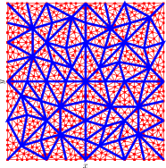
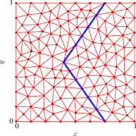
Figure 3. An unstructured mesh with the interface $\Gamma$ (blue-dashed).

the number of iterations grows like ${h}^{-1/2}$ when we refine the mesh, provided that $\gamma=\frac{1}{2}(1+\sqrt{h})$, as our new theoretical analysis predicts.

Mesh size	$h_{0}$	$h_{0}/2$	$h_{0}/4$	$h_{0}/8$
# iterations	1057	1297	1951	2734

Table 1. Convergence of OSM for 110 subdomains ($h$-dependence).

4.2. Dependence on the polynomial degree

We next illustrate how the contraction factor of Algorithm 3.2 depends on the polynomial degree. First, we choose a two subdomain configuration with a non-straight interface (see Figure 3 right) for $\Omega=(0,1)^{2}$. Then we choose $\gamma=\frac{1}{2}(1+\frac{1}{k})$, $\eta=1$ and run Algorithm 3.2. We expect from our analysis to obtain $\rho\leq 1-O(\frac{1}{k})$, which is indeed observed in Figure 4.

Then we choose $\Omega$ to be the domain in Figure 1 with seven subdomains (including floating ones). We observe in Figure 4 that the number of iterations grows like $O(k^{-1})$, which is expected from our analysis.

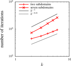
Figure 4. Convergence of the OSM with respect to polynomial degree.

4.3. Effect of the time-step on convergence

In Section 3.3 we showed how the convergence of the two subdomain algorithm is affected by the choice of $\eta$. In Table 2 we see the number of iterations required to reach a given accuracy for different choices of $\eta$. The domain decomposition setting is same as Figure 3 (right).

	$h_{0}$	$h_{0}/2$	$h_{0}/4$	$h_{0}/8$
case $\eta=O(1)$	103	214	405	820
case $\eta=O(h^{-1})$	41	60	83	115
case $\eta=O(h^{-2})$	16	16	15	14

Table 2. Convergence of Algorithm 3.2 with $\gamma=1$ and different choices of $\eta$.

Observe that for $\eta=O(1)$, the number of iterations grows like $O(h^{-1})$ while for $\eta=O(h^{-1})$ we observe $O(h^{-1/2})$ for the growth of the number of iterations. If we choose $\eta=O(h^{-2})$, we obtain an optimal solver since the number of iterations does not depend on the mesh parameter.

In Table 3 we compare the theoretical estimate in (3.28) with the numerical experiments of Table 2.

	experiments	theoretical
case $\eta=O(1)$	$1-h$	$1-h$	(sharp)
case $\eta=O(h^{-1})$	$1-\sqrt{h}$	$1-h$	(not sharp)
case $\eta=O(h^{-2})$	$1-c$	$1-c$	(sharp)

Table 3. Comparison of contraction factors between the theoretical estimates of Section 3.3 and the numerical experiments.

Note that the estimates of Section 3.3 can capture the optimality of the solver when $\eta=O(h^{-2})$. However it is not sharp when $\eta=O(h^{-1})$.

We perform the same experiment with four subdomains on $\Omega=(0,1)^{2}$ and we choose $\eta=O(h^{-2})$. We see in Table 4 that the number of iterations remains constant as we refine the mesh.

Mesh size	$h_{0}$	$h_{0}/2$	$h_{0}/4$	$h_{0}/8$
# iterations	144	157	168	164

Table 4. Convergence of OSM for four subdomains with $\eta=O(h^{-2})$.

Finally we perform numerical experiments on the weak scaling of the algorithm. According to Corollary 3.5, when $\tau=O(H^{2})$ and the ratio $H/h$ is constant, i.e., we refine the mesh and the subdomain at the same time, one obtains a contraction factor independent of the mesh size. This can be achieved also using ASM applied to FEM. In Table 5, we illustrate the convergence of the OSM on a sequence of fine and coarse meshes such that the ratio $H/h$ remains constant.

Mesh size	$h_{0}$	$h_{0}/2$	$h_{0}/4$	$h_{0}/8$
# iterations	105	95	99	104

Table 5. Convergence of OSM while the ratio $H/h$ is constant with $\eta=O(H^{-2})$.

5. Conclusion

We designed and analyzed an optimized Schwarz method (OSM) for the solution of elliptic problems discretized by hybridizable interior penalty (IPH) discontinuous Galerkin methods. Our results are a generalization of the two subdomain analysis in [11] to the case of many subdomains, and we also study theoretically for the first time the influence of the polynomial degree of IPH discretizations, and the effect of the time-step on the convergence of OSM when solving parabolic problems. We derived the optimized parameter and corresponding contraction factor for various asymptotic regimes of the mesh and subdomain size and the time-step, and obtained scalability without a coarse space and also mesh independent solvers in certain specific regimes. We validated our theoretical results by numerical experiments. The optimized contraction factor shows a clear advantage of OSM compared to the additive Schwarz method applied to the primal formulation, e.g., see the one-level ASM version of [8] or [1]. The next step is to design and analyze a coarse correction for these OSM solvers applied to IPH in the regimes where Algorithm 3.2 is not scalable.

Appendix A Proof of some estimates

We now prove several technical estimates we used in the analysis of the OSM for IPH. For all subdomains when $\eta\geq 0$ we have the inequalites

(A.1) $$\mu{\|\varphi_{i}\|}_{\Gamma_{i}}^{2}-a_{i}(v_{i},v_{i}) \geq c\,{\|(v_{i},\varphi_{i})\|}_{i}^{2}, \forall\varphi_{i}\in\Lambda_{i},v_{i}=\mathcal{H}_{i}(\varphi_{i}),$$

(A.2) $$\big{(}1-c(h,H,k)\big{)}\mu{\|\varphi_{i}\|}_{\Gamma_{i}}^{2} \geq a_{i}(v_{i},v_{i}), \forall\varphi_{i}\in\Lambda_{i},v_{i}=\mathcal{H}_{i}(\varphi_{i}),$$

where

$$c(h,H,k):=\left\{\begin{array}[]{ll}\frac{h}{H}\frac{1}{k^{2}}&\text{for non-floating subdomains},\\ 0&\text{for floating subdomains}.\end{array}\right.$$

We also have for all subdomains when $\eta>0$ the estimate

(A.3) $${\|\mathcal{R}_{i}(\varphi_{i})\|}_{\Gamma_{i}}^{2}\leq\Big{(}(2\gamma-1)^{2}C(H,\eta)+\mu^{-1}\Big{)}{\|(u_{i},\varphi_{i})\|}_{i}^{2},$$

where

$$C(H,\eta):=\left\{\begin{array}[]{ll}H&\text{for non-floating subdomain},\\ \frac{1}{H\eta}&\text{for floating subdomain}.\end{array}\right.$$

We first recall an inequiality related to the coercivity of the IPH method, that is

(A.4) $$a_{i}(v_{i},v_{i})+2a_{i\Gamma}(v_{i},\varphi_{i})+\mu{\|\varphi_{i}\|}_{\Gamma_{i}}^{2}\geq c{\|(v_{i},\varphi_{i})\|}_{i}^{2},\quad\forall\varphi_{i}\in\Lambda_{i},v_{i}\in V_{h,i}.$$

For a proof see [18, 11]. The proof of (A.1) is obtained by choosing $v_{i}:=\mathcal{H}_{i}(\varphi_{i})$ in (A.4) and recalling the definition of the harmonic extension which leads to $a_{i}(v_{i},v_{i})+a_{i\Gamma}(v_{i},\varphi_{i})=0$. Substituting this into (A.4) proves (A.1).

In order to prove (A.2) we decompose the proof into two parts: floating subdomains and non-floating ones. Recall that ${\|(\cdot,\cdot)\|}_{i}$ is a semi-norm for floating subdomains if $\eta=0$, i.e., the kernel consists of constant functions. This concludes the proof for floating subdomains with $c(h,H,k)=0$. For non-floating subdomains we recall a trace inequality for totally discontinuous functions, see [11, Lemma 3.6] and [3]:

Lemma A.1.

Let $\varphi_{i}\in\Lambda_{i}$ and $u_{i}\in V_{h,i}$. Let $H_{i}$ be the diameter of a non-floating subdomain. Then we have

(A.5) $$\frac{c}{H_{i}}{\|\varphi_{i}\|}_{\Gamma_{i}}^{2}\leq{\|\nabla u_{i}\|}_{\Omega_{i}}^{2}+\mu{\|[\![u_{i}]\!]\|}_{\mathcal{E}_{i}\setminus\Gamma_{i}}^{2}+\mu{\|u_{i}-\varphi_{i}\|}_{\Gamma_{i}}^{2}.$$

We then substitute (A.5) into (A.1) and recalling the definition of ${\|(u_{i},\varphi_{i})\|}_{i}$ proves (A.2) for non-floating subdomains with $c(h,H,k)=\frac{h}{H}\frac{1}{k^{2}}$.

We now prove (A.3). Recall that the $\textrm{L}^{2}$-norm of the $\mathcal{R}_{i}(\cdot)$ is a norm while ${\|(\cdot,\cdot)\|}_{i}$ is only a semi-norm for floating subdomains if $\eta=0$. Therefore (A.3) makes sense for $\eta>0$. Recall the definition of the $\mathcal{R}_{i}(\cdot)$ operator,

$$\mathcal{R}_{i}(\varphi_{i}):=\gamma\varphi_{i}-\frac{1}{2\mu}\Big{(}\mu-\frac{\partial{}}{\partial{{\boldsymbol{n}}_{i}}}\Big{)}u_{i}=\big{(}\gamma-\frac{1}{2}\big{)}\varphi_{i}+\frac{1}{2}\big{(}\varphi_{i}-u_{i}\big{)}+\frac{1}{2\mu}\frac{\partial{u_{i}}}{\partial{{\boldsymbol{n}}_{i}}},$$

where $u_{i}=\mathcal{H}_{i}(\varphi_{i})$. We then take the $\textrm{L}^{2}$-norm over $\Gamma_{i}$ and apply the triangle inequality,

(A.6) $$\begin{array}[]{rcl}{\|\mathcal{R}_{i}(\varphi_{i})\|}_{\Gamma_{i}}^{2}&\leq&4\big{(}\gamma-\frac{1}{2}\big{)}^{2}{\|\varphi_{i}\|}_{\Gamma_{i}}^{2}+4(\frac{1}{2})^{2}{\|\varphi_{i}-u_{i}\|}_{\Gamma_{i}}^{2}+4\big{(}\frac{1}{2\mu}\big{)}^{2}{\|\frac{\partial{u_{i}}}{\partial{{\boldsymbol{n}}_{i}}}\|}_{\Gamma_{i}}^{2},\\ &\leq&4\big{(}\gamma-\frac{1}{2}\big{)}^{2}{\|\varphi_{i}\|}_{\Gamma_{i}}^{2}+{\|\varphi_{i}-u_{i}\|}_{\Gamma_{i}}^{2}+c\mu^{-1}{\|\nabla u_{i}\|}_{\Omega_{i}}^{2},\\ &\leq&4\big{(}\gamma-\frac{1}{2}\big{)}^{2}{\|\varphi_{i}\|}_{\Gamma_{i}}^{2}+c\mu^{-1}\big{(}\mu{\|\varphi_{i}-u_{i}\|}_{\Gamma_{i}}^{2}+{\|\nabla u_{i}\|}_{\Omega_{i}}^{2}\big{)}.\end{array}$$

For non-floating subdomains we use Lemma A.1 for the first term on the right-hand side and obtain

(A.7) $$\Big{(}(2\gamma-1)^{2}H_{i}+c\mu^{-1}\Big{)}\eta{\|u_{i}\|}_{\Omega_{i}}^{2}+{\|\mathcal{R}_{i}(\varphi_{i})\|}_{\Gamma_{i}}^{2}\leq\Big{(}(2\gamma-1)^{2}H_{i}+c\mu^{-1}\Big{)}{\|(u_{i},\varphi_{i})\|}_{i}^{2}.$$

For floating subdomains we use a trace inequality by Feng and Karakashian [8, Lemma 3.1],

(A.8) $${\|u_{i}\|}_{\Gamma_{i}}^{2}\leq c\Big{[}H_{i}^{-1}{\|u_{i}\|}_{\Omega_{i}}^{2}+H_{i}\big{(}{\|\nabla u_{i}\|}_{\Omega_{i}}^{2}+h^{-1}{\|[\![u_{i}]\!]\|}_{\mathcal{E}_{i}\setminus\Gamma_{i}}^{2}\big{)}\Big{]}.$$

We then invoke ${\|\varphi_{i}\|}_{\Gamma_{i}}^{2}\leq 2{\|u_{i}\|}_{\Gamma_{i}}^{2}+2{\|u_{i}-\varphi_{i}\|}_{\Gamma_{i}}^{2}$, use (A.8) and recall the definition of ${\|(u_{i},\varphi_{i})\|}$ to obtain

$${\|\varphi_{i}\|}_{\Gamma_{i}}^{2}\leq\frac{C}{H_{i}\eta}{\|(u_{i},\varphi_{i})\|}_{i}^{2}.$$

Substituting this estimate back into (A.6) yields

(A.9) $${\|\mathcal{R}_{i}(\varphi_{i})\|}_{\Gamma_{i}}^{2}\leq\Big{(}(2\gamma-1)^{2}\cdot C\cdot(H_{i}\eta)^{-1}+c\mu^{-1}\Big{)}{\|(u_{i},\varphi_{i})\|}_{i}^{2}.$$

References

• [1] Paola F. Antonietti and Blanca Ayuso, Schwarz domain decomposition preconditioners for discontinuous galerkin approximations of elliptic problems: non-overlapping case, ESAIM: Mathematical Modelling and Numerical Analysis 41 (2007), 21–54.
• [2] Douglas N. Arnold, Franco Brezzi, Bernardo Cockburn, and L. Donatella Marini, Unified analysis of discontinuous Galerkin methods for elliptic problems, SIAM J. Numer. Anal. 39 (2001/02), no. 5, 1749–1779. MR 1885715 (2002k:65183)
• [3] Susanne C. Brenner, Poincaré-Friedrichs inequalities for piecewise $H^{1}$ functions, SIAM J. Numer. Anal. 41 (2003), no. 1, 306–324. MR 1974504 (2004d:65140)
• [4] Xiao-Chuan Cai, Additive Schwarz algorithms for parabolic convection-diffusion equations, Numerische Mathematik 60 (1991), no. 1, 41–61 (English).
• [5] Paul Castillo, Performance of discontinuous Galerkin methods for elliptic PDEs, SIAM J. Sci. Comput. 24 (2002), no. 2, 524–547. MR 1951054 (2003m:65200)
• [6] Bernardo Cockburn, Jayadeep Gopalakrishnan, and Raytcho Lazarov, Unified hybridization of discontinuous Galerkin, mixed, and continuous Galerkin methods for second order elliptic problems, SIAM J. Numer. Anal. 47 (2009), no. 2, 1319–1365. MR 2485455 (2010b:65251)
• [7] Richard E. Ewing, Junping Wang, and Yongjun Yang, A stabilized discontinuous finite element method for elliptic problems, Numer. Linear Algebra Appl. 10 (2003), no. 1-2, 83–104, Dedicated to the 60th birthday of Raytcho Lazarov. MR 1964287 (2004b:65181)
• [8] Xiaobing Feng and Ohannes A. Karakashian, Two-level additive Schwarz methods for a discontinuous Galerkin approximation of second order elliptic problems, SIAM J. Numer. Anal. 39 (2001), no. 4, 1343–1365 (electronic). MR 1870847 (2003a:65113)
• [9] Martin J. Gander, Optimized Schwarz methods, SIAM J. Numer. Anal. 44 (2006), no. 2, 699–731 (electronic). MR 2218966 (2007d:65121)
• [10] Martin J. Gander and Soheil Hajian, Block Jacobi for discontinuous Galerkin discretizations: no ordinary Schwarz methods, Domain Decomposition Methods in Science and Engineering XXI, Lect. Notes Comput. Sci. Eng. Springer (2013).
• [11] Martin J. Gander and Soheil Hajian, Analysis of Schwarz methods for a hybridizable discontinuous Galerkin discretization, SIAM Journal on Numerical Analysis 53 (2015), no. 1, 573–597.
• [12] Martin J Gander and Felix Kwok, Best Robin parameters for optimized Schwarz methods at cross points, SIAM Journal on Scientific Computing 34 (2012), no. 4, A1849–A1879.
• [13] by same author, On the applicability of Lions’ energy estimates in the analysis of discrete optimized Schwarz methods with cross points, Domain Decomposition Methods in Science and Engineering XX, Springer, 2013, pp. 475–483.
• [14] Martin J. Gander and Kévin Santugini, Cross-points in domain decomposition methods with a finite element discretization, revised (2015).
• [15] Claude J. Gittelson, Ralf Hiptmair, and Ilaria Perugia, Plane wave discontinuous galerkin methods: Analysis of the h-version, ESAIM: Mathematical Modelling and Numerical Analysis 43 (2009), 297–331.
• [16] Soheil Hajian, An optimized Schwarz algorithm for discontinuous Galerkin methods, Domain Decomposition Methods in Science and Engineering XXII (2014).
• [17] Soheil Hajian, Analysis of Schwarz methods for discontinuous Galerkin discretizations, Ph.D. thesis, 06/04 2015, ID: unige:75225.
• [18] Christoph Lehrenfeld, Hybrid discontinuous Galerkin methods for incompressible flow problems, Master’s thesis, RWTH Aachen, 2010.
• [19] P.-L. Lions, On the Schwarz alternating method. III. A variant for nonoverlapping subdomains, Third International Symposium on Domain Decomposition Methods for Partial Differential Equations (Houston, TX, 1989), SIAM, Philadelphia, PA, 1990, pp. 202–223. MR 1064345 (91g:65226)
• [20] Sébastien Loisel, Condition number estimates for the nonoverlapping optimized Schwarz method and the 2-Lagrange multiplier method for general domains and cross points, SIAM Journal on Numerical Analysis 51 (2013), no. 6, 3062–3083.
• [21] LiZhen Qin, ZhongCi Shi, and XueJun Xu, On the convergence rate of a parallel nonoverlapping domain decomposition method, Sci. China Ser. A 51 (2008), no. 8, 1461–1478. MR 2426076 (2010d:65364)
• [22] Lizhen Qin and Xuejun Xu, On a parallel Robin-type nonoverlapping domain decomposition method, SIAM Journal on Numerical Analysis 44 (2006), no. 6, pp. 2539–2558 (English).
• [23] Lizhen Qin and Xuejun Xu, Optimized Schwarz methods with Robin transmission conditions for parabolic problems, SIAM Journal on Scientific Computing 31 (2008), no. 1, 608–623.
• [24] Andrea Toselli and Olof Widlund, Domain decomposition methods—algorithms and theory, Springer Series in Computational Mathematics, vol. 34, Springer-Verlag, Berlin, 2005. MR 2104179 (2005g:65006)