Entanglement-assisted quantum metrology

Abstract

Entanglement-assisted quantum communication employs pre-shared entanglement between sender and receiver as a resource. We apply the same framework to quantum metrology, introducing shared entanglement between the preparation and the measurement stage, namely using some entangled ancillary system that does not interact with the system to be sampled. This is known to be useless in the noiseless case, but was recently shown to be useful in the presence of noise. Here we detail how and when it can be of use. For example, surprisingly it is useful when randomly time sharing two channels where ancillas do not help (depolarizing). We show that it is useful for all levels of noise for many noise models and propose a simple optical experiment to test these results.

Entanglement-assisted communication sd ; shor ; shor1 employs pre-shared entanglement between sender and receiver in addition to the signals sent through the channel. This doubles the capacity of a noiseless channel, as illustrated in the well known superdense coding protocol sd , and is even more beneficial in the presence of noise shor1 ; dc-noise . Here we apply the same framework to quantum metrology qmetr ; rev1 ; phase-comp ; rev2 ; dowling2008quantum , which studies how quantum effects may aid parameter estimation.

A quantum parameter estimation is composed of three stages (Fig. 1a): the preparation stage, where some probe systems are initialized; the sampling stage, where the probes interact with the system to be sampled (this interaction encodes the parameter on the probes); the measurement stage, where the probes are measured and the outcome is processed to yield the parameter estimate. Entanglement-assisted quantum metrology (Fig. 1b) refers to the scenario in which the probes are entangled with an ancilla that does not participate to the sampling stage (similar ideas have also been studied in the context of noisy channel estimation fujiwara ; fujiwara2 ). Then at the measurement stage a joint measurement is performed between probes and ancilla. It was recently realized that this is useful in the presence of noise rafal ; qeckraus ; qecarrad ; qeckessler ; haine ; kolodynski2013efficient , although it was known to be useless in the noiseless case qmetr . Here we detail how entangled ancillas can be used, what are the gains one can achieve and which explicit measurement strategies can achieve such gains, analyzing the most important qubit channels. We also propose a simple experiment that can test our results.

The entanglement-assisted scenario should not be confused with the generic use of entanglement in quantum estimation, that has been extensively studied previously, e.g. caves ; caves1 ; qmetr ; nph ; dinani ; shaji ; chiara ; ian ; chavez ; cillis , showing how entangled probes achieve better precision than unentangled ones. It is also different from the application of quantum error correction to metrology qeckraus ; qecarrad ; qeckessler ; qecozeri where all the systems are involved in the interaction (Fig. 1c), although some scenarios analyzed in Refs. qeckraus ; qecarrad ; qeckessler ; qecozeri go beyond this conventional quantum error correction scheme. Instead, in the entanglement-assisted scenario, the ancilla does not interact and can be considered as noiseless, if we suppose (as is often the case) that the noise is relevant especially during the interaction stage. This translates into a reduced noise acting on the global state and a reduced resource count: indeed in quantum metrology the resource count refers to the number of times that the probed system is sampled rev2 . So, the entangled ancillas should be accounted for as separate resources, as is done in quantum communication sd ; shor ; shor1 .

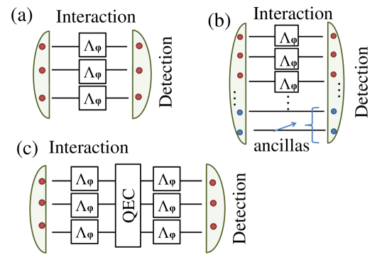
Figure 1: (a) Conventional quantum parameter estimation: probes are prepared in a joint entangled state, they interact (independently) with the probed system through a noisy map $\Lambda_{\varphi}$, and they are jointly measured. (b) Entanglement-assisted parameter estimation: ancillary systems are employed that do not interact with the probed system. (c) QEC schemes: after the interaction the errors are corrected and, possibly, the probes interact again.

We will detail the increase in achievable precision in the presence of an entangled ancilla with respect to the one achievable in its absence, instead of dealing with the issue of whether one can beat the standard quantum limit or achieve the Heisenberg bound. Indeed, it is known that the Heisenberg scaling cannot be achieved asymptotically for many of these noise models guta ; davidovich ; jarzna ; durkin ; alipour , although it can often be achieved in the non-asymptotic regime brauns ; alipour1 ; geo600 . Interestingly, it has been pointed out qeckraus ; qecarrad ; qeckessler that the Heisenberg scaling can be recovered through entanglement-assisted metrology even asymptotically in the very special case of orthogonal noise, even though only a lower scaling is achieved in the absence of ancillas chavez . However a general analysis of entanglement-assisted metrology was lacking up to now: our results show the attainable precision enhancement for the case of the Pauli channels (including the fully depolarizing case) and of the amplitude damping. Moreover, dephasing and erasure noise do not allow for any enhancement in the entanglement-assisted scenario, although entanglement among the probes is helpful rafal . Our analysis then concludes the study of entanglement-assisted estimation for all relevant qubit channels.

Most previous literature studies the precision through the quantum Cramer-Rao (QCR) bound, with the promise that such a lower bound to precision is significant because it is asymptotically achievable. However, since we want achieveability in the non-asymptotic regime, we must provide estimation strategies and prove that they achieve the QCR, at least in a feedback scenario feedb1 ; feedb2 . Indeed, both the QCR and the error in the employed strategy may depend on the unknown parameter to be estimated gdurkin , but a feedback strategy converges exponentially to the “sweet spot” dowling1 , so that it has only a logarithmic cost in terms of resources feedb1 . Even though the rigorous way to determine phase errors is the Holevo variance holevo ; ph-gen , as is usually done in the literature we will use the customary variance, since the two match for sufficiently precise estimation strategies.

The QCR holevo ; helstrom ; caves ; caves1 is a lower bound to the precision $\Delta\varphi$ of the estimation of a parameter $\varphi$: under reasonable hypotheses, $\Delta\varphi\geqslant 1/\sqrt{\nu J(\rho_{\varphi})}$ where $\nu$ is the number of times the estimation is repeated, and $J$ is the quantum Fisher information (QFI) associated to the global state $\rho_{\varphi}$ of probes and ancillas (after the interaction $\Lambda_{\varphi}$ with the probed system). The QFI is

$$J(\rho_{\varphi})=\sum_{j,k:\lambda_{j}+\lambda_{k}\neq 0}{2|\langle j|\rho^{\prime}_{\varphi}|k\rangle|^{2}}/({\lambda_{j}+\lambda_{k}})\;,$$ (1)

where $\rho^{\prime}_{\varphi}=\partial\rho_{\varphi}/\partial\varphi$, $\lambda_{j}$ and $|j\rangle$ are the eigenvalues and eigenvectors of $\rho_{\varphi}$. The map $\Lambda_{\varphi}$ encodes the phase parameter $\varphi$ onto the probes: $\rho_{\varphi}=\Lambda_{\varphi}[\rho]$, where $\rho$ is the initial state. Without loss of generality, for qubit channels we suppose that the phase is encoded onto the computational basis by the unitary $U_{\varphi}=|0\rangle\langle 0|+e^{i\varphi}|1\rangle\langle 1|$. For the sake of simplicity we will consider situations where the noise maps ${\cal E}$ acts after $U_{\varphi}$, namely $\Lambda_{\varphi}={\cal E}\circ U_{\varphi}$. If the noise map and $U_{\varphi}$ do not commute, this is an important restriction of our analysis (required to make the problem tractable, as nontrivial effects arise otherwise chavez ), but it is not a restriction for the erasure, amplitude damping and depolarizing noise models which commute with $U_{\varphi}$.

To find the best bound, one must maximize the QFI, which in general depends both on the input state $\rho$ and on the unknown parameter $\varphi$. The former optimization depends on the noise map, the latter can be taken care of using feedback mechanisms feedb1 ; feedb2 ; gdurkin ; dowling1 . For all noise maps, we can use the convexity of QFI fujiwara to choose a pure input state $\rho=|\psi\rangle\langle\psi|$. Indeed, supposing that $\rho=\sum_{j}\lambda_{j}|j\rangle\langle j|$, we have $J(\rho_{\varphi})=J(\sum_{j}\lambda_{j}\Lambda_{\varphi}[|j\rangle\langle j|])\leqslant\sum_{j}\lambda_{j}J(\Lambda_{\varphi}[|j\rangle\langle j|])$. (The QFI is not convex if $\lambda_{j}$ depended on $\varphi$, but an extended convexity still holds alipour1 .)

I Amplitude damping

We start by analyzing the amplitude damping channel with Kraus operators

$$A_{0}=\left(\begin{array}[]{cc}1&0\\ 0&\sqrt{1-\eta}\\ \end{array}\right),\ A_{1}=\left(\begin{array}[]{cc}0&\sqrt{\eta}\\ 0&0\\ \end{array}\right),$$ (2)

where $\eta$ is the probability of decay $|1\rangle\to|0\rangle$. This map is agnostic on the direction of the $x$ and $y$ axis of the Bloch sphere: a rotation around the $z$ axis leaves $A_{0}$ unchanged and adds an inconsequential phase factor to $A_{1}$. Thus we can optimize the single-probe input state among the family $\epsilon|0\rangle+\sqrt{1-\epsilon^{2}}|1\rangle$. The optimal state has $\epsilon=1/\sqrt{2}$, and its QFI is $1-\eta$. To show that entanglement-assisted strategies perform better, we compare this QFI with the one of an entangled state of probe and ancilla $|\psi_{\gamma}\rangle=\gamma|00\rangle+\sqrt{1-\gamma^{2}}|11\rangle$. This state might not be the optimal state for the entanglement-assisted strategy, but it outperforms the previous one. Indeed its corresponding output state $(\Lambda_{\varphi}\otimes\openone)[|\psi_{\gamma}\rangle\langle\psi_{\gamma}|]$ (where the map acts only on the probe qubit and not on the ancilla) has a QFI of ${4(1-\eta)}/{(\sqrt{1-\eta}+1)^{2}}$ (also shown by kolodynski2013efficient ), if one optimizes over $\gamma$ for each $\eta$. Even the simple choice $\gamma=1/\sqrt{2}$ is advantageous for all $\eta$ as its QFI is ${2(1-\eta)}/({2-\eta})$. These QFIs are compared in Fig. 2a.

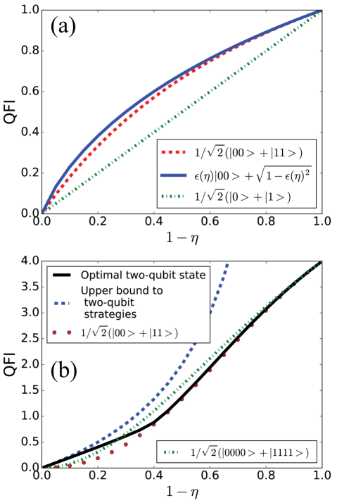
Figure 2: Amplitude damping channel. (a) Single qubit probe: QFI of the optimal ancilla-assisted state $|\psi_{\gamma}\rangle$ (continuous), the maximally entangled state of probe and ancilla (dashed) and single qubit state (dotted). For all $\eta$ the ancilla-assisted strategies have better QFI. (b) Two-qubit probes: the optimal two-qubit state (continuous line) and the “noon” state (which is optimal only in the noiseless case, red circles) are compared to a genuinely entangled four-qubit state (two probe and two ancilla qubits, dot-dashed line). We also plot the upper bound to the ancilla-less estimation with two probes from durkin (dashed), which is achievable in the high noise regime (where the dashed and continuous lines superimpose). The ancilla-assisted strategy beats any entangled-probe strategies for $\eta<0.7$. The state can be further optimized.

One observable that achieves the QCR bound for the last QFI is ${O}=\Pi_{\psi}+2\ket{\Phi^{+}}\bra{\Phi^{+}}$, with $\ket{\Phi^{+}}=\frac{1}{\sqrt{2}}(\ket{00}+\ket{11})$ and $\Pi_{\psi}=(\ket{01}\bra{01}+\ket{10}\bra{10})$. Indeed, measuring the observable $O$, the error on $\varphi$ is

$$\Delta\varphi^{2}=\frac{\Delta O^{2}}{(d\braket{O}/d\varphi)^{2}}=\frac{1-\eta/2-(1-\eta)\cos^{2}{\varphi}}{(1-\eta)\sin^{2}{\varphi}}.$$ (3)

This expression is optimized for $\varphi=\pi/2$, where the Cramer-Rao bound of the optimal single-probe state is beaten performing Bell measurements between probe and ancilla. As discussed above, we can perform the optimization $\varphi\to\pi/2$ using a feedback strategy feedb1 ; feedb2 ; gdurkin ; dowling1 that uses an additional phase factor feedb1 in the interferometer to drive the global phase to this “sweet spot”.

The ancilla-assisted advantage persists also when we use entangled probes. The case without ancillas was analyzed in durkin where an upper bound $N(1-\eta)/\eta$ to the Fisher information was given, which is achievable in the high-noise regime $N\eta/(1-\eta)\gg 1$.

In the case of two qubit probes, one can also perform a numerical optimization of the QFI on generic two-qubit states (presented in Fig. 2b, solid line).

Interestingly, the performance of the optimal state is similar to the “noon” state $|\Phi^{+}\rangle$, which is known to be optimal in the noiseless case. However, all these strategies can be beaten by using ancillas (as was noted also in rafal , although no explicit example was presented there). In Fig. 2b, dotted-dashed line, we show the performance of a the four-qubit NOON state $(|0000\rangle+|1111\rangle)/\sqrt{2}$ of two probes and two ancillas: it beats the optimal state of two probes for noise levels $\eta\approx 0.7$, where its QFI is $\frac{8(\eta-1)^{2}\left(2(\eta-1)^{2}\cos(8\varphi)+(\eta-2)\eta((\eta-2)\eta+2)+2\right)}{((\eta-2)\eta+2)^{3}}$, which is optimal for $\varphi=\frac{2\pi{n}}{8}$, where $n$ is an integer. One observable that achieves the QCR for the single-qubit probe is $O=2\ket{N}\bra{N}+\Sigma$, where $\ket{N}=1/\sqrt{2}(\ket{0000}-\ket{1111})$ and $\Sigma=\ket{0011}\bra{0011}+\ket{0111}\bra{0111}+\ket{1011}\bra{1011}$. Note that this particular four-qubit state is not necessary optimal.

II General Pauli

The generalized Pauli channel is described by

$$\Lambda[\rho]=(1-{p_{1}-p_{2}-p_{3}})\rho+{p_{1}}\sigma_{x}\rho\sigma_{x}^{\dagger}+{p_{2}}\sigma_{y}\rho\sigma_{y}^{\dagger}+{p_{3}}\sigma_{z}\rho\sigma_{z}^{\dagger},$$ (4)

with $\sigma_{x}$, $\sigma_{y}$, $\sigma_{z}$ Pauli matrices, and $p_{1}$, $p_{2}$ and $p_{3}$ probabilities. Two special Pauli channels are the dephasing and the depolarizing noise. Dephasing noise corresponds to $p_{1}=p_{2}=0$ in (4) and it was proved that ancillas offer no advantage over the unentangled probe rafal : for both cases the optimal QFI of a single-qubit probe is $(1-2p_{3})^{2}$. Depolarising noise corresponds to having $p_{1}=p_{2}=p_{3}\equiv p/4$ in (4): it describes an isotropic loss of coherence . As was also shown in kolodynski2013efficient , in this case ancillas do help: indeed for a single-qubit probe, the optimal state is $1/\sqrt{2}(\ket{0}+\ket{1})$ where the QFI is $(1-p)^{2}$, whereas the QFI for a probe maximally entangled with an ancilla is $2(1-p)^{2}/(2-p)$, which is always greater .

This result is very surprising since the depolarizing channel can be seen as a time-sharing (with probability $1-p$) of a noiseless channel and a channel where the state of the probe is replaced by a maximally mixed state $\openone/2$ (useless for estimation). For both of these channels the use of an ancilla gives no advantage: the ancilla becomes important only when they are randomly time-shared.

One observable that achieves the QCR for the single-qubit probe is $O=\ket{+}\bra{+},\ket{+}=1/\sqrt{2}(\ket{0}+\ket{1})$, and for the ancilla-assisted case, $O=\Pi_{\psi}+2\ket{\Phi^{+}}\bra{\Phi^{+}}$ (identical with the one for the ADC).

Even though dephasing and depolarizing channels commute with the unitary $U_{\varphi}$, in general the Pauli channel does not: we will consider the case where the noise acts only after $U_{\varphi}$. For a single qubit probe in the generic initial state $\epsilon|0\rangle+\sqrt{1-\epsilon^{2}}e^{i\alpha}|1\rangle$, the QFI is

$$J^{(na)}_{\varphi} = 4\epsilon^{2}\left(\epsilon^{2}-1\right)[{p_{1}}(2-4{p_{3}})+4{p_{3}}-4{p_{3}}({p_{2}}+{p_{3}})$$

$$-1-2{p_{1}}^{2}-2(-1+{p_{2}}){p_{2}}\;$$

$$+2({{p_{1}}}-{{p_{2}}})\cos(2(\alpha+\varphi))({{p_{1}}}+{{p_{2}}}+2{{p_{3}}}-1)]$$

($na$ stands for “no ancilla”), which is maximized for $\epsilon=1/\sqrt{2}$ for all $\varphi$, and (as before) one can optimize over $\varphi$ (or, equivalently, $\alpha$) using a feedback strategy. To prove that the presence of an ancilla is beneficial, we consider a maximally entangled state $\frac{1}{\sqrt{2}}(\ket{00}+\ket{11})$ of probe and ancilla. In this case the QFI is

$$J^{(a)}_{\varphi}=\frac{({p_{1}}-{p_{2}})^{2}}{{p_{1}}+{p_{2}}}+\frac{({p_{1}}+{p_{2}}+2{p_{3}}-1)^{2}}{1-{p_{1}}-{p_{2}}}.$$ (6)

We performed a numerical search over the parameter space ${p_{1}},{p_{2}},{p_{3}}$. For all possible values of ${p_{1}}+{p_{2}}+{p_{3}}\leq 1$, the expression in Eq.(6) is larger than that of Eq. (II) for all $\alpha$.

To illustrate this, the comparison between (II) and (6) is shown in Fig. 3, for the case when ${p_{1}}=0$ and $\alpha+\varphi=0$. The probe-ancilla observable $\hat{O}=\ket{\Phi^{-}}\bra{\Phi^{-}}+\ket{\Psi^{-}}\bra{\Psi^{-}}$ achieves the QCR bound relative to the QFI of (6), with $\ket{\Phi^{-}}=\frac{1}{\sqrt{2}}(\ket{00}-\ket{11})$, $\ket{\Psi^{-}}=\frac{1}{\sqrt{2}}(\ket{01}-\ket{10})$.

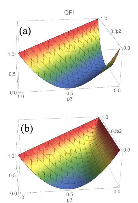
Figure 3: General Pauli channel (for the case $p_{1}=0$). (a) The optimized QFI for a single-probe in Eq(II), $\epsilon=1/\sqrt{2},\alpha+\varphi=0$ and (b) the QFI of the ancilla strategy in Eq. (6).

Note that when $p_{1}({p_{2}})=0$ and $p_{1}(p_{2})+p_{3}=1$, the QFI is unity: this represents the case of orthogonal noise when the ancilla strategy can recover the full information on the phase even in the presence of noise, as was pointed out in qeckraus ; qecarrad ; qeckessler .

III Experiment proposal

We propose here an experimental scheme to implement our proposal, based on the use of a single photon, where two qubits are encoded in the path and polarisation degrees of freedom.

Such a scheme, that can simulate the ancilla-assisted strategy, is shown in Fig.4. The experiment uses a single photon which is prepared in a polarization-path entangled state as follows and the noise acts on the polarization degree of freedom. The initial polarisation state of the photon in this scheme is $\frac{1}{\sqrt{2}}(\ket{H}+\ket{V})$. A polarizing beam splitter (PBS) then transmits $\ket{H}$ and reflects $\ket{V}$. Therefore, PBS1 acts as an effective CNOT gate and puts into a polarization-path entangled state $1/\sqrt{2}(\ket{Ha}+\ket{Vb})$ (red solid = a, blue dashed = b). The state is then transformed according to the unitary $U_{\varphi}$ and the noisy channel. Different noise models can be added, e.g. using the techniques implemented in exps . If the bit is flipped, the flipped component is directed by PBS2 and PBS3 onto another path, which interfere at BS2. The half wave plate (HWP) rotates V polarization to H so that they interfere at the 50:50 beam splitter (BS). The which-arm statistics after the BS are effective projective Bell measurements in this basis. That is, at BS1, the outputs correspond to projecting onto $1/\sqrt{2}(\ket{Ha}\pm\ket{Vb})$, and at BS2, $1/\sqrt{2}(\ket{Va}\pm\ket{Hb})$. This scheme is easily implementable with present-day technologies, e.g. in exps similar schemes were experimentally realized and controlled noise was introduced in an ancilla-assisted scenario for different purposes.

IV Conclusions

In conclusion, we have studied the role of entangled ancillas in metrology for the important classes of qubit noise models. We have shown that, for a single probe, in the presence of amplitude damping, depolarizing noise as well as general Pauli noise, an entanglement-assisted scheme provides an advantage in the efficiency of phase measurement over the unentangled case for all ranges of noise regimes. We also derived the optimal measurement procedures which achieve the Cramer-Rao bound.

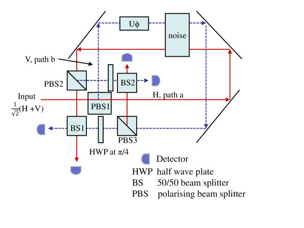
Figure 4: An experimental scheme to perform phase estimation using the ancilla-assisted scheme. See text for details.

We acknowledge useful feedback from Rafal Demkowicz-Dobrzanski.

References

- (1) C.H. Bennett, S.J. Wiesner, Phys. Rev. Lett. 69, 2881 (1992).
- (2) C. H. Bennett, P. W. Shor, J. A. Smolin, and A. V. Thapliyal, Phys. Rev. Lett. 83, 3081 (1999).
- (3) C. H. Bennett, P. W. Shor, J. A. Smolin, and A. V. Thapliyal, IEEE Trans. Inform. Theory 48, 2637 (2002), Eprint quant-ph/0106052.
- (4) Z. Shadman, H. Kampermann, C. Macchiavello and D. Bruss, New J. Phys. 12, 073042 (2010).
- (5) V. Giovannetti, S. Lloyd, and L. Maccone, Phys. Rev. Lett. 96, 010401 (2006).
- (6) V. Giovannetti, S. Lloyd, and L. Maccone, Science 306, 1330 (2004).
- (7) W. van Dam, G. M. D’Ariano, A. Ekert, C. Macchiavello and M. Mosca, Phys. Rev. Lett. 98, 090501 (2007).
- (8) V. Giovannetti, S. Lloyd, and L. Maccone, Nature Photonics 5, 222 (2011).
- (9) J. P. Dowling, Contemporary physics 49, 125 (2008).
- (10) A. Fujiwara, Phys. Rev. A 63, 042304 (2001); A. Fujiwara, Phys. Rev. A 70 012317 (2004).
- (11) A. Fujiwara, H. Imai , J. Phys. A: Math. Gen. 36 8093 (2003)
- (12) R. Demkowicz-Dobrzanski, L. Maccone, Phys. Rev. Lett. 113, 250801 (2014).
- (13) W. Dür, M. Skotiniotis, F. Fröwis, B. Kraus, Phys. v. Lett. 112, 080801 (2014).
- (14) G. Arrad, Y. Vinkler, D. Aharonov, and A. Retzker, Phys. Rev. Lett. 112, 150801 (2014).
- (15) E. M. Kessler, I. Lovchinsky, A. O. Sushkov, and M. D. Lukin, Phys. Rev. Lett. 112, 150802 (2014).
- (16) S. A. Haine,S. S. Szigeti, Phys. Rev. A 92, 032317 (2015), S A. Haine, S S. Szigeti, M. D. Lang,C. M. Caves, Phys. Rev. A 91 041802, (2015)
- (17) R. Demkowicz-Dobrzański, J. Kolodynski New Journal of Physics, 15, 073043 (2013).
- (18) S. L. Braunstein and C. M. Caves, Phys. Rev. Lett. 72, 3439 (1994).
- (19) S. L. Braunstein, C. M. Caves, and G. Milburn, Annals Phys. 247, 135 (1996).
- (20) G. Y. Xiang, B. L. Higgins, D. W. Berry, H. M. Wiseman, G. J. Pryde, Nature Photonics 5, 43 (2011).
- (21) H. T. Dinani and D. W. Berry, Phys. Rev. A 90, 023856 (2014).
- (22) A. Shaji and C. M. Caves, Phys. Rev. A 76, 032111 (2007).
- (23) S. F. Huelga, C. Macchiavello, T. Pellizzari, A.K. Ekert, M.B. Plenio, J.I. Cirac, Phys. Rev. Lett. 79, 3865 (1997).
- (24) M. Kacprowicz, R. Demkowicz-Dobrzanski, W. Wasilewski, K. Banaszek, I. A. Walmsley, Nature Photonics 4, 357 (2010).
- (25) R. Chaves, J. B. Brask, M. Markiewicz, J. Kolodyński, A. Acín, Phys. Rev. Lett. 111, 120401 (2013).
- (26) L. Maccone and G. De Cillis, Phys. Rev. A 79, 023812 (2009).
- (27) R. Ozeri arXiv:1310.3432 (2013).
- (28) R. Demkowicz-Dobrzanski, J. Kolodynski, M. Guta, Nature communications 3, 1063 (2012).
- (29) B. Escher, R. de Matos Filho, and L. Davidovich, Nature Physics 7, 406 (2011).
- (30) M. Jarzyna, R. Demkowicz-Dobrzanski, New J. Phys. 17, 013010 (2015).
- (31) S.I. Knysh, E.H. Chen, G.A. Durkin, arXiv:1402.0495 (2014).
- (32) S. Alipour, M. Mehboudi, A.T. Rezakhani Phys. Rev. Lett. 112, 120405 (2014).
- (33) S. L. Braunstein Phys. Rev. Lett. 69, 3598 (1992).
- (34) S. Alipour, A. T. Rezakhani Phys. Rev. A 91, 042104 (2015).
- (35) R. Demkowicz-Dobrzanski, K. Banaszek, R. Schnabel Phys. Rev. A 88, 041802(R) (2013).
- (36) D. W. Berry, H. M. Wiseman Phys. Rev. Lett. 85, 5098 (2000); D. W. Berry, H. M. Wiseman, J. K. Breslin Phys. Rev. A 63, 053804 (2001); D. Berry, arXiv quant-ph/0202136 (2002).
- (37) A. Hentschel, B.C. Sanders Phys. Rev. Lett. 104, 063603 (2010); A. Hentschel, B.C. Sanders Phys. Rev. Lett. 107, 233601 (2011).
- (38) G.A. Durkin, J.P. Dowling Phys. Rev. Lett. 99, 070801 (2007).
- (39) K.P. Seshadreesan, S. Kim, J. P. Dowling, H. Lee Phys. Rev. A 87, 043833 (2013).
- (40) A.S. Holevo, Probabilistic and statistical aspects of quantum theory (North Holland pub. co., Amsterdam, 1982).
- (41) For the general case see also: G.M. D’Ariano, C. Macchiavello and M.F. Sacchi, Phys. Lett. A 248, 103 (1998).
- (42) C. W. Helstrom, “Quantum Detection and Estimation Theory,” (Academic Press, New York, 1976).
- (43) A. Chiuri et al, Phys. Rev. Lett. 107, 253602 (2011); A. Orieux et al, Phys. Rev. Lett. 111, 220501 (2013); A. Orieux et al, Phys. Rev. Lett. 115, 160503 (2015).