An efficient Exact-PGA algorithm for constant curvature manifolds

Abstract

Manifold-valued datasets are widely encountered in many computer vision tasks. A non-linear analog of the PCA, called the Principal Geodesic Analysis (PGA) suited for data lying on Riemannian manifolds was reported in literature a decade ago. Since the objective function in PGA is highly non-linear and hard to solve efficiently in general, researchers have proposed a linear approximation. Though this linear approximation is easy to compute, it lacks accuracy especially when the data exhibits a large variance. Recently, an alternative called exact PGA was proposed which tries to solve the optimization without any linearization. For general Riemannian manifolds, though it gives better accuracy than the original (linearized) PGA, for data that exhibit large variance, the optimization is not computationally efficient. In this paper, we propose an efficient exact PGA for constant curvature Riemannian manifolds (CCM-EPGA). CCM-EPGA differs significantly from existing PGA algorithms in two aspects, (i) the distance between a given manifold-valued data point and the principal submanifold is computed analytically and thus no optimization is required as in existing methods. (ii) Unlike the existing PGA algorithms, the descent into codimension-1 submanifolds does not require any optimization but is accomplished through the use of the Rimeannian inverse Exponential map and the parallel transport operations. We present theoretical and experimental results for constant curvature Riemannian manifolds depicting favorable performance of CCM-EPGA compared to existing PGA algorithms. We also present data reconstruction from principal components and directions which hasn’t been presented in literature in this setting.

1 Introduction

Principal Component Analysis (PCA) is a widely used dimensionality reduction technique in Science and Engineering. PCA however requires the input data to lie in a vector space. With the advent of new technologies and wide spread use of sophisticated feature extraction methods, manifold-valued data have become ubiquitous in many fields including Computer Vision, Medical Imaging and Machine Learning. A nonlinear version of PCA, called Principal Geodesic Analysis (PGA), for data lying on Riemannian manifolds was introduced in [8].

Since the objective function of PGA is highly nonlinear and hard to solve in general, researchers proposed a linearized version of PGA [8]. Though this linearized PGA, hereafter referred to as PGA, is computationally efficient, it lacks accuracy for data with large spread/variance. In order to solve the objective function exactly, some researchers proposed to solve the original objective function (not the approximation) and called it exact PGA [24]. While exact PGA attempts to solve this complex nonlinear optimization problem, it is however computationally inefficient. Though it is not possible to efficiently and accurately solve this optimization problem for a general manifold, however, for manifolds with constant sectional curvature, we formulate an efficient and exact PGA algorithm, dubbed CCM-EPGA. It is well known in geometry, by virtue of Killing-Hopf theorem, [4] that any non-zero constant curvature manifold is isomorphic to either the hypersphere ($\mathbf{S}^{N}$) or the hyperbolic space ($\mathbf{H}^{N}$), hence in this work, we present the CCM-EPGA formulation for ($\mathbf{S}^{N}$) and ($\mathbf{H}^{N}$). Our formulation has several applications to Computer Vision and Statistics including directional data [20] and color spaces [18]. Several other applications of hyperbolic geometry are, shape analysis [29], electrical Impedence Tomography, Geoscience imaging [27], brain morphometry [28], catadiaoptric vision [3] etc.

In order to depict the effectiveness of our proposed CCM-EPGA, we use the average projection error as defined in [24]. We also report the computational time comparison of the CCM-EPGA with the PGA [8] and the exact PGA [24]. Several variants of PGA exist in literature and we briefly mention a few here. In [22], authors computed the principal geodesics without approximation only for a special Lie group, $SO(3)$. Geodesic PCA (GPCA) [13, 12] solves a different optimization function namely, optimizing the projection error along geodesics. The authors in [12] minimize the projection error instead of maximizing variance in geodesic subspaces (defined later in the paper). GPCA does not use a linear approximation, but it is restricted to manifolds where a closed form expression for the geodesics exists. More recently, a probabilistic version of PGA called PPGA was presented in [30], which is a nonlinear version of PPCA [26]. None of these methods attempt to compute the solution to the exact PGA problem defined in [24].

The rest of the paper is organized as follows. In Section 2, we present the formulation of PGA. We also discuss the details of the linearized version of PGA [8] and exact PGA [24]. Our formulation of CCM-EPGA is presented in Section 2. We present experimental results of CCM-EPGA algorithm along with comparisons to exact PGA and PGA in Section 3. In addition to synthetic data experiments, we present the comparative performance of CCM-EPGA on two real data applications. In Section 4, we present the formulation for reconstruction of data from principal directions and components in this nonlinear setting. Finally, in section 5, we draw conclusions.

2 Principal Geodesic Analysis

Principal Component Analysis (PCA) [16] is a well known and widely used statistical method for dimensionality reduction. Given a vector valued dataset, it returns a sequence of linear subspaces that maximize the variance of the projected data. The $k^{th}$ subspace is spanned by the principal vectors $\{\mathbf{v}_{1},\mathbf{v}_{2},\cdots,\mathbf{v}_{k}\}$ which are mutually orthogonal. PCA is well suited for vector-valued data sets but not for manifold-valued inputs. A decade ago, the nonlinear version called the Principal Geodesic Analysis (PGA) was developed to cope with manifold-valued inputs [8]. In this section, first, we briefly describe this PGA algorithm, then, we show the key modification performed in [24] to arrive at what they termed as the exact PGA algorithm. We then motivate and present our approach which leads to an efficient and novel algorithm for exact PGA on constant curvature manifolds (CCM-EPGA).

Let $M$ be a Riemannian manifold. Let’s suppose we are given a dataset, $X=\{x_{1},\cdots,x_{n}\}$, where $x_{j}\in M$. Let us assume that the finite sample Fréchet mean [9] of the data set exists and be denoted by $\mu$. Let $V_{k}$ be the space spanned by mutually orthogonal vectors (principal directions) $\{\mathbf{v}_{1},\cdots,\mathbf{v}_{k}\}$, $\mathbf{v}_{j}\in T_{\mu}M,\forall j$. Let $S_{k}$ be the $k^{th}$ geodesic subspace of $T_{\mu}M$, i.e., $S_{k}=Exp_{\mu}(V_{k})$, where $Exp$ is the Riemannian exponential map (see [4] for definition). Then, the principal directions, $\mathbf{v}_{i}$ are defined recursively by

$$\mathbf{v}_{i} = \displaystyle\operatorname*{arg\,max}_{\|\mathbf{v}\|=1,\mathbf{v}\in V_{i-1}^{\bot}}\frac{1}{n}\displaystyle\sum_{j=1}^{n}d^{2}(\mu,\Pi_{S_{i}}(x_{j}))$$ (1)

$$S_{i} = Exp_{\mu}(span{V_{i-1},\mathbf{v}_{i}})$$ (2)

where $d(x,y)$ is the geodesic distance between $x\in M$ and $y\in M$, $\Pi_{S}(x)$ is the point in $S$ closest to $x\in M$.

The PGA algorithm on $M$ is summarized in Alg. 1.

Algorithm 1 The PGA algorithm on manifold $M$

1:Given dataset $X=\{x_{1},\cdots,x_{n}\}\in M$, and $1\leq L\leq dim(M)$

2:Compute the FM, $\mu$, of $X$ [1]

3:Set $k\leftarrow 1$

4:Set $\{\bar{x}_{1}^{0},\cdots,\bar{x}_{n}^{0}\}$ $\leftarrow$ $\{x_{1},\cdots,x_{n}\}$

5:while  $k\leq L$  do

6:     Solve $\mathbf{v}_{k}=\displaystyle\operatorname*{arg\,max}_{\|\mathbf{v}\|=1,\mathbf{v}\in T_{\mu}M,\mathbf{v}\in V_{k-1}^{\bot}}\frac{1}{n}\displaystyle\sum_{j=1}^{n}d^{2}(\mu,\Pi_{S_{k}}(x_{j}))$ as in Eq. (1).

7:     Project $\{\bar{x}_{1}^{k-1},\cdots,\bar{x}_{n}^{k-1}\}$ to a $k$ co-dimension one submanifold $Z$ of $M$, which is orthogonal to the current geodesic subspace.

8:     Set the projected points to $\{\bar{x}_{1}^{k},\cdots,\bar{x}_{n}^{k}\}$

9:     $k\leftarrow k+1$

10:end while

2.1 PGA and exact PGA

In Alg. 1 (lines $6-7$), as the projection operator $\Pi$ is hard to compute, hence a common alternative is to locally linearize the manifold. This approach [8] maps all data points on the tangent space at $\mu$, and as tangent plane is a vector space, one can use PCA to get the principal directions. This simple scheme is an approximation of the PGA. This motivated the researchers to ask the following question: Is it possible to do PGA, i.e., solve Eq. (1) without any linearization? The answer is yes. But, computation of the projection operator, $\Pi_{S}(x)$, i.e., the closest point of $x$ in $S$ is computationally expensive. In [24], Sommer et al. give an alternative definition of PGA, i.e., they minimize the average squared reconstruction error, i.e., $d^{2}(x_{j},\Pi_{S_{i}}(x_{j}))$ instead of $d^{2}(\mu,\Pi_{S_{i}}(x_{j}))$ in eqns. (1). They use an optimization scheme to compute this projection. Further, they termed their algorithm, exact PGA, as it does not require any linearization. However, their optimization scheme is in general computationally expensive and for a data set with large variance, convergence is not guaranteed. Hence, for large variance data, their exact PGA is still an approximation as it might not converge. This motivates us to formulate an accurate and computationally efficient exact PGA.

2.2 Efficient and accurate exact PGA

In this paper, we present an analytic expression for the projected point and design an effective way to project data points on to the co-dimension $k$ submanifold (as in 1, line $7$). An analytic expression is in general not possible to derive for arbitrary Riemannian manifolds. However, for constant curvature Riemannian manifolds, i.e., $\mathbf{S}^{N}$ (positive constant curvature) and $\mathbf{H}^{N}$ (negative constant curvature), we derive an analytic expression for the projected point and devise an efficient algorithm to project data points on to a co-dimension $k$ submanifold. Both these manifolds are quite commonly encountered in Computer Vision [10, 19, 3, 28, 29] as well as many other fields of Science and Engineering. The former more so than the latter. Eventhough, there are applications that can be naturally posed in hyperbolic spaces (e.g., color spaces in Vision [18], catadiaoptric images [3] etc.), their full potential has not yet been exploited in Computer Vision research as much as in the former case.

We first present some background material for the $N$-dimensional spherical and hyperbolic manifolds and then derive an analytical expression of the projected point.

2.2.1 Basic Riemannian Geometry of $\mathbf{S}^{N}$

• Geodesic distance: The geodesic distance between $\psi,\bar{\psi}\in\mathbf{S}^{N}$ is given by, $d(\psi,\bar{\psi})=\arccos(\psi^{t}\bar{\psi})$.

• Exponential Map: Given a vector $\mathbf{v}\in T_{\psi}\mathbf{S}^{N}$, the Riemannian Exponential map on $\mathbf{S}^{N}$ is defined as $Exp_{\psi}(\mathbf{v})=\cos(|\mathbf{v}|)\psi+\sin(|\mathbf{v}|)\mathbf{v}/|\mathbf{v}|$. The Exponential map gives the point which is located on the great circle along the direction defined by the tangent vector $\mathbf{v}$ at a distance $|\mathbf{v}|$ from $\psi$.

• Inverse Exponential Map: The tangent vector $\mathbf{v}\in T_{\psi}\mathbf{S}^{N}$ directed from $\psi$ to $\bar{\psi}$ is given by, $Exp^{-1}_{\psi}(\bar{\psi})=\frac{\theta}{\sin(\theta)}(\bar{\psi}-\psi\cos(\theta))$ where, $\theta=d(\psi,\bar{\psi})$. Note that, the inverse exponential map is defined everywhere on the hypersphere except at the antipodal points.

2.2.2 Basic Riemannian Geometry of $\mathbf{H}^{N}$

The hyperbolic $N$-dimensional manifold can be embedded in $\mathbf{R}^{N+1}$ using three different models. In this discussion, we have used the hyperboloid model [14]. In this model, $\mathbf{H}^{N}$ is defined as $\mathbf{H}^{N}=\{\mathbf{x}=(x_{1},\cdots,x_{N+1})^{t}\in\mathbf{R}^{N+1}|<x,x>_{H}=-1,x_{1}>0\}$, where the inner product on $\mathbf{H}^{N}$, denoted by $<x,y>_{H}$ is defined as $<x,y>_{H}=-x_{1}*y_{1}+\sum_{i=2}^{N+1}(x_{i}*y_{i})$.

• Geodesic distance: The geodesic distance between $\psi,\bar{\psi}\in\mathbf{H}^{N}$ is given by, $d(\psi,\bar{\psi})=\cosh^{-1}(-<\psi,\bar{\psi}>_{H})$.

• Exponential Map: Given a vector $\mathbf{v}\in T_{\psi}\mathbf{H}^{N}$, the Riemannian Exponential map on $\mathbf{H}^{N}$ is defined as, $Exp_{\psi}(\mathbf{v})=\cosh(|\mathbf{v}|)\psi+\sinh(|\mathbf{v}|)\mathbf{v}/|\mathbf{v}|$.

• Inverse Exponential Map: The tangent vector $\mathbf{v}\in T_{\psi}\mathbf{H}^{N}$ directed from $\psi$ to $\bar{\psi}$ is given by $Exp^{-1}_{\psi}(\bar{\psi})=\frac{\theta}{\sinh(\theta)}(\bar{\psi}-\psi\cosh(\theta))$ where, $\theta=d(\psi,\bar{\psi})$.

For the rest of this paper, we consider the underlying manifold, $M$, as a constant curvature Riemannian manifold, i.e., $M$ is diffeomorphic to either $\mathbf{S}^{N}$ or $\mathbf{H}^{N}$, where $N=dim(M)$ [4]. Let $\psi,\bar{\psi}\in M$, $\mathbf{v}\in T_{\bar{\psi}}M$. Further, let $y(\mathbf{v},\psi)$ be defined as the projection of $\psi$ on the geodesic submanifold defined by $\bar{\psi}$ and $\mathbf{v}$. Now, we will derive a closed form expression for $y(\mathbf{v},\psi)$ in the case of $\mathbf{S}^{N}$ and $\mathbf{H}^{N}$.

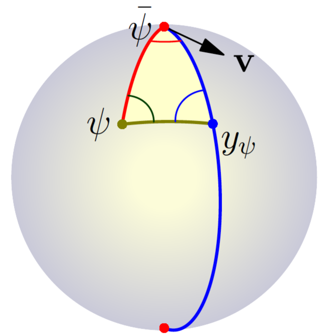
Figure 1: Analytic expression for the projected point on the Sphere.

2.3 Analytic expression for $y(\mathbf{v},\psi)$ on $\mathbf{S}^{N}$

Theorem 1.

Let $\psi\in\mathbf{S}^{N}$ and $\mathbf{v}\in T_{\bar{\psi}}\mathbf{S}^{N}$. Then the projection of $\psi$ on the geodesic submanifold defined by $\bar{\psi}$ and $\mathbf{v}$, i.e., $y(\mathbf{v},\psi)$ is given by:

$$y(\mathbf{v},\psi)=\cos(\arctan\Bigg{(}\frac{(<\mathbf{v},\psi>)/(<\psi,\bar{\psi}>)}{|\mathbf{v}|}\Bigg{)})\bar{\psi}$$

$$+\sin(\arctan\Bigg{(}\frac{(<\mathbf{v},\psi>)/(<\psi,\bar{\psi}>)}{|\mathbf{v}|}\Bigg{)})\mathbf{v}/|\mathbf{v}|$$ (3)

Proof.

Consider the spherical triangle shown in Fig. 1, $\bigtriangleup\bar{\psi}\psi y_{\psi}$, where $y_{\psi}=y(\mathbf{v},\psi)$. Let, $a=d(\bar{\psi},y_{\psi})$, $b=d(y_{\psi},\psi)$ and $c=d(\psi,\bar{\psi})$. Also, let $A=\angle\bar{\psi}\psi y_{\psi}$, $B=\angle\psi\bar{\psi}y_{\psi}$, $C=\angle\bar{\psi}y_{\psi}\psi$. Clearly, since $y_{\psi}$ is the projected point , $C=\pi/2$. So,

$$\cos B=\frac{<\frac{c}{\sin c}(\psi-\bar{\psi}\cos c),\mathbf{v}>}{c|\mathbf{v}|}$$

$$=\frac{\frac{<\mathbf{v},\psi>}{\sin c}-\cot c<\mathbf{v},\bar{\psi}>}{|\mathbf{v}|}$$ (4)

Here, $<.,.>$ denotes the Euclidean inner product, where both $\psi$ and $\mathbf{v}$ are viewed as points in $\mathbf{R}^{N+1}$, i.e., the ambient space. Note that, $<\mathbf{v},\bar{\psi}>=0$, as $\mathbf{v}\in T_{\bar{\psi}}\mathbf{S}^{N}$. From spherical trigonometry, we know that $\tan a=\cos B\tan c$.

$$\therefore\cos B\tan c = \frac{\frac{<\mathbf{v},\psi>}{\cos c}}{|\mathbf{v}|}$$

$$= \frac{(<\mathbf{v},\psi>)/(<\psi,\bar{\psi}>)}{|\mathbf{v}|}$$

$$\therefore a=\arctan\Bigg{(}\frac{(<\mathbf{v},\psi>)/(<\psi,\bar{\psi}>)}{|\mathbf{v}|}\Bigg{)}$$ (5)

Hence, using the Exponential map, we can show that $y_{\psi}$ is given by,

$$y_{\psi}=\cos(a)\bar{\psi}+\sin(a)\mathbf{v}/|\mathbf{v}|$$ (6)

∎

Analogously, we can derive the formula for $y(\mathbf{v},\psi)$ on $\mathbf{H}^{N}$, $\mathbf{v}\in T_{\bar{\psi}}\mathbf{H}^{N}$.

Theorem 2.

Let $\psi\in\mathbf{H}^{N}$ and $\mathbf{v}\in T_{\bar{\psi}}\mathbf{H}^{N}$. Then the projection of $\psi$ on the geodesic submanifold defined by $\bar{\psi}$ and $\mathbf{v}$, i.e., $y(\mathbf{v},\psi)$ is given by:

$$y_{\psi}=\cosh(a)\bar{\psi}+\sinh(a)\mathbf{v}/|\mathbf{v}|$$ (7)

where,

$$a=\tanh^{-1}\Bigg{(}\frac{(<\mathbf{v},\psi>_{H})/(-<\psi,\bar{\psi}>_{H})}{|\mathbf{v}|}\Bigg{)}$$

.

Proof.

As before, consider the hyperbolic triangle shown in, $\bigtriangleup\bar{\psi}\psi y_{\psi}$, where $y_{\psi}=y(\mathbf{v},\psi)$. Let, $a=d(\bar{\psi},y_{\psi})$, $b=d(y_{\psi},\psi)$ and $c=d(\psi,\bar{\psi})$. Also, let $A=\angle\bar{\psi}\psi y_{\psi}$, $B=\angle\psi\bar{\psi}y_{\psi}$, $C=\angle\bar{\psi}y_{\psi}\psi$. Clearly, since $y_{\psi}$ is the projected point , $C=\pi/2$. Then, $B$ is the angle between $Log_{\bar{\psi}}(\psi)$ and $\mathbf{v}$. Hence,

$$\cosh B = \frac{\frac{<\mathbf{v},\psi>_{H}}{\sinh c}-\coth c<\mathbf{v},\bar{\psi}>_{H}}{|\mathbf{v}|}$$ (8)

Then, from hyperbolic trigonometry, as $\tanh a=\cosh B\tanh c$, we get

$$a=\tanh^{-1}\Bigg{(}\frac{(<\mathbf{v},\psi>_{H})/(-<\psi,\bar{\psi}>_{H})}{|\mathbf{v}|}\Bigg{)}$$ (9)

Note that, as the arc length between $\bar{\psi}$ and $y_{\psi}$ is $a$, hence, using Exponential map, we can show that $y_{\psi}=\cosh(a)\bar{\psi}+\sinh(a)\mathbf{v}/|\mathbf{v}|$.

∎

Given the closed form expression of the projected point, now we are in a position to devise an efficient projection algorithm (for line $7$ in Alg. 1), which is given in Alg. 2. Note that, using Alg. 2, data points on the current submanifold are projected to a submanifold of dimension one less, which is needed by the PGA algorithm in line 6. Also note that, in order to ensure existence and uniqueness of FM, we have restricted the data points to be within a geodesic ball of convexity radius $<\pi/2$ [1].

Algorithm 2 Algorithm for projecting the data points to a co-dimension one submanifold

1:Input: a data point $x_{i}\in\mathbf{S}^{N}(\mathbf{H}^{N})$, a geodesic submanifold defined at $\mu$ and $\mathbf{v}\in T_{\mu}\mathbf{S}^{N}(T_{\mu}\mathbf{H}^{N})$, and $y(\mathbf{v},x_{i})$ which is the projection of $\psi$ on to the geodesic submanifold.

2:Output: $\bar{x}_{i}$ which is the projection of the data point $x_{i}$ to a subspace, $\mathbf{S}^{N-1}(\mathbf{H}^{N-1})$, which is orthogonal to the current geodesic submanifold.

3:Step 1. Evaluate the tangent vector, $\mathbf{v}_{i}\in T_{y(\mathbf{v},x_{i})}\mathbf{S}^{N}(T_{y(\mathbf{v},x_{i})}\mathbf{H}^{N})$ directed towards $x_{i}$ using the Inverse Exponential Map. It is clear that $\mathbf{v}_{i}$ is orthogonal to $\mathbf{v}$.

4:Step 2. Parallel transport $\mathbf{v}_{i}$ to $\mu$. Let $\mathbf{v}_{i}^{\mu}$ denote the parallel transported vector. The geodesic submanifold defined by $\mu$ and $\mathbf{v}_{i}^{\mu}$ is orthogonal to geodesic submanifolds obtained from the previous steps in Alg. 1.

5:Step 3. Set $\bar{x}_{i}\leftarrow y(\mathbf{v}_{i}^{\mu},x_{i})$

Note that in order to descend to the codimension-1 submanifolds, we use step-1 and step-2 instead of the optimization method used in the exact PGA algorithm of [24].

3 Experimental Results

In this section, we present experiments demonstrating the performance of CCM-EPGA compared to PGA [8] and exact PGA [24]. We used the average projection error, defined in [24], as a measure of performance in our experiments. The average projection error is defined as follows. Let $\{x_{i}\}_{i=1}^{n}$ be data points on a manifold $M$. Let $\mu$ be the mean of the data points. Let, $\mathbf{v}$ be the first principal direction and $S=Exp_{\mu}(\mathbf{v})$. Then the error $(E)$ is defined as follows:

$$E=\frac{1}{n}\sum_{i=1}^{n}d^{2}(x_{i},\Pi_{S}(x_{i}))$$ (10)

where $d(.,.)$ is the geodesic distance function on $M$. We also present the computation time for each of the three algorithms. All the experimental results reported here were obtained on a desktop with a single 3.33 GHz Intel-i7 CPU with 24 GB RAM.

3.1 Comparative performance of CCM-EPGA on Synthetic data

In this section, we present the comparitive performance of CCM-EPGA on several synthetic datasets. For each of the synthetic data, we have reported the average projection error and computation time for all three PGA algorithms in Table 1. All the four datasets are on $S^{2}$ and the Fréchet mean is at the ”north pole”. For all the datasets, samples are in the northern hemisphere to ensure that the Fréchet mean is unique. Data_1 and Data_2 are generated by taking samples along a geodesic with a slight perturbation. The last two datasets are constructed by drawing random samples on the northern hemisphere. In addition, data points from Data_1 are depicted in Fig. 2. The first principal direction is also shown (black for CCM-EPGA, blue for PGA and red for exact PGA). Further, we also report the data variance for these synthetic datasets. By examining the results, it’s evident that for data with low variance, the significance of CCM-EPGA in terms of projection error is marginal, while for high variance data, CCM-EPGA yields significantly better accuracy. Also, CCM-EPGA is computationally very fast in comparison to exact PGA. The results in Table 1 indicate that CCM-EPGA outperforms exact PGA in terms of efficiency and accuracy. Although, the required time for PGA is less than that of CCM-EPGA, in terms of accuracy, CCM-EPGA dominates PGA.

Data	Var.	CCM-EPGA		PGA		exact PGA
		avg. proj. err.	Time(s)	avg. proj. err.	Time(s)	avg. proj. err.	Time(s)
Data_1	2.16	$\mathbf{1.13e-04}$	0.70	0.174	$\mathbf{0.46}$	2.54e-02	14853
Data_2	0.95	$\mathbf{5.87e-02}$	0.27	0.59	$\mathbf{0.12}$	0.59	84.38
Data_3	7.1e-03	$\mathbf{2.33e-03}$	0.19	0.55	$\mathbf{0.05}$	0.55	16.87
Data_4	5.9e-02	$\mathbf{0.27}$	0.33	0.37	$\mathbf{0.14}$	0.37	71.84

Table 1: Comparison results on synthetic datasets

Figure 2: Synthetic data (Data_1) on $S^{2}$

3.2 Comparative performance on point-set data ($\mathbf{S}^{N}$ example)

In this section, we depict the performance of the proposed CCM-EPGA on 2D point-set data. The database is called GatorBait-100 dataset [21]. This dataset consists of $100$ images of shapes of different fishes. From each of these images of size $20\times 200$, we first extract boundary points, then we apply the Schrödinger distance transform [7] to map each of these point sets on a hypersphere ($S^{3999}$). Hence, this data consists of $100$ point-sets each of which lie on $S^{3999}$. As before, we have used the average projection error [24], to measure the performance of algorithms in the comparisons. Additionally, we report the computation time for each of these PGA algorithms. We used the code available online for exact PGA [23]. This online implementation is not scalable to large (even moderate) number of data points, and furhter requires the computation of the Hessian matrix in the optimization step, which is computationally expensive. Hence, for this real data application on the high dimensional hypersphere, we could not report the results for the exact PGA algorithm. Though one can use a Sparse matrix version of the exact PGA code, along with efficient parallelization to make the exact PGA algorithm suitable for moderately large data, we would like to point out that since our algorithm does not need such modifications, it clearly gives CCM-EPGA an advantage over exact PGA from a computational efficiency perspective. In terms of accuracy, it can be clearly seen that CCM-EPGA outperforms exact PGA from the results on synthetic datasets. Both average projection error and computational time on GatorBait-100 dataset are reported in Table 2. This result demonstrates accuracy of CCM-EPGA over the PGA algorithm with a marginal sacrifice in efficiency but significant gains in accuracy.

Method	avg. proj. error	Time(s)
CCM-EPGA	$\mathbf{2.83e-10}$	$0.40$
PGA	$9.68e-02$	$\mathbf{0.28}$

Table 2: Comparison results on Gator-Bait database

3.3 PGA on population of gaussian distributions ($\mathbf{H}^{N}$ example)

In this section, we propose a novel scheme to compute principal geodesic submanifolds for the manifold of gaussian densities. Here, we use concepts from information geometry presented in [2], specifically, the Fisher information matrix [17] to define a metric on this manifold [6]. Consider a normal density $f(.|\boldsymbol{\theta})$ in an $n-$dimensional space, with parameters represented by $\boldsymbol{\theta}$. Then the ${ij}^{th}$ entry of the $n\times n$ Fisher matrix, denoted by $g_{ij}$, is defined as follows:

$$g_{ij}(\boldsymbol{\theta})=\int_{\mathbf{R}}f(x|\boldsymbol{\theta})\frac{\partial lnf(x|\boldsymbol{\theta})}{\partial\theta_{i}}\frac{\partial lnf(x|\boldsymbol{\theta})}{\partial\theta_{j}}dx$$ (11)

For example, for a univariate normal density $f(.|\mu,\sigma)$, the fisher information matrix is

$$(g_{ij}(\mu,\sigma))=\begin{pmatrix}\frac{1}{\sigma^{2}}&0\\ 0&\frac{2}{\sigma^{2}}\end{pmatrix}$$ (12)

So, the metric is defined as follows:

$$<u,v>=u^{t}Gv$$ (13)

where $G=(g_{ij})$ is the Fisher information matrix. Now, consider the parameter space for the univariate normal distributions. The parameter space is $H_{F}={(\mu,\sigma)\in\mathbf{R}^{2}|\sigma>0}$, i.e., positive half space, which is the Hyperbolic space, modeled by the Poincaré half-plane, denoted by $\mathbf{P}^{2}$. We can define a bijection $F_{1}:H_{F}\rightarrow\mathbf{P}^{2}$ as $F(\mu,\sigma)=(\frac{\mu}{\sqrt{2}},\sigma)$. Hence, the univariate normal distributions can be parametrized by the $2-$dimensional hyperbolic space. Moreover, there exists a diffeomorphsim between $\mathbf{P}^{2}$ and $\mathbf{H}^{2}$ (the mapping is analogous to stereographic projection for $\mathbf{S}^{N}$), thus, we can readily use the formulation in Section 2 to compute principal geodesic submanifold on the manifold of univariate normal distributions.

Motivated by the above formulation, we ask the following question: Does there exist a similar relation for multivariate normal distributions? The answer is no in general. But if the multivariate distributions have diagonal covariance matrix, (i.e., independent uncorrelated variables in the mutivariate case), the above relation between $\mathbf{P}^{2}$ and $\mathbf{H}^{2}$ can be generalized. Consider an $N-$dimensional normal distribution parametrized by $(\boldsymbol{\mu},\Sigma)$ where $\boldsymbol{\mu}=(\mu_{1},\cdots,\mu_{N})^{t}$ and $\Sigma$ is a diagonal positive definite matrix (i.e., $\Sigma_{ij}=\sigma_{i}$, if $i=j$, else $\Sigma_{ij}=0$). Then, analogous to the univariate normal distribution case, we can define a bijection $F_{N}:H^{N}_{F}\rightarrow\mathbf{P}^{2N}$ as follows:

$$F_{N}(\boldsymbol{\mu},\Sigma)=(\frac{\mu_{1}}{\sqrt{2}},\sigma_{1},\cdots,\frac{\mu_{N}}{\sqrt{2}},\sigma_{N})$$ (14)

Hence, we can use our formulation in Section 2 since there is a diffeomorphism between $\mathbf{P}^{2N}$ and $\mathbf{H}^{2N}$. But, for general non-diagonal $N-$dimensional covariance matrix space, $SPD(N)$, the above formulation does not hold. This motivated us to go one step further to search for a parametrization of $SPD(N)$ where we can use the above formulation. In [15], authors have used the Iwasawa coordinates to parametrize $SPD(N)$. Using the Iwasawa coordinates [25], we can get a one-to-one mapping between $SPD(N)$ and the product manifold of $PD(N)$ and $U(N-1)$, where $PD(N)$ is manifold of $N-$dimensional diagonal positive definite matrix and $U(N-1)$ is the space of $(N-1)-$dimensional upper triangular matrices, which is isomorphic to $R^{N(N+1)/2}$. We have used the formulation in [25], as discussed below.

Let $Y=V_{N}\in SPD(N)$, then we can use Iwasawa decomposition to represent $V_{N}$ as a tuple $(V_{N-1},x_{N-1},w_{N-1})$. And repeating the following partial Iwasawa decomposition:

$$V_{N}=\begin{pmatrix}I&x_{N-1}\\ 0&1\end{pmatrix}^{T}\begin{pmatrix}V_{N-1}&0\\ 0&w_{N-1}\end{pmatrix}$$ (15)

where $w_{N-1}>0$ and $x_{N-1}\in\mathbf{R}^{N-1}$. We get the following vectorized expression: $V_{N}\mapsto(((w_{0},x_{1}^{t},w_{1}),x_{2}^{t},w_{2}),\cdots,x_{N-1}^{t},w_{N-1})$. Note that as each of $w_{i}$ is $>0$, we can construct a positive definite diagonal matrix with $i^{th}$ diagonal entry being $w_{i}$. And as each $x_{i}$ is in $\mathbf{R}^{i}$, we will arrange them columnwise to form a upper triangular matrix. Thus, for $PD(N)$, we can use our formulation for the hyperboloid model of the hyperbolic space given in Section 2, and the standard PCA can be applied for $R^{N(N+1)/2}$.

We now use the above formulation to compute the principal geodesic submanifolds for a covariance descriptor representation of Brodatz texture dataset [5]. Similar to our previous experiment on point-set data, in this experiment, we report the average projection error and computation time. We adopt a similar procedure as in [11] to derive the covariance descriptors for the texture images in the Brodatz database. Each $256\times 256$ texture image is first partitioned into $64$ non-overlapping $8\times 8$ blocks. Then, for each block, the covariance matrix ($FF^{T}$) is summed over the blocks. Here, the covariance matrix is computed from the feature vector $F=\bigg{(}I,|\frac{\partial I}{\partial x}|,|\frac{\partial I}{\partial y}|,|\frac{\partial^{2}I}{\partial x^{2}}|,|\frac{\partial^{2}I}{\partial y^{2}}|\bigg{)}^{t}$. We make the covariance matrix positive definite by adding a small positive diagonal matrix. Then, each image is represented as a normal distribution with zero mean and this computed covariance matrix. Then, we used the above formulation to map each normal distribution on to $\mathbf{H}^{10}$. The comparative results of CCM-EPGA with PGA and exact PGA are presented in Table 3. The results clearly indicate efficiency and accuracy of CCM-EPGA compared to PGA and exact PGA algorithms.

Method	avg. proj. error	Time(s)
CCM-EPGA	$\mathbf{7.73e-03}$	$0.09$
PGA	$0.14$	$\mathbf{0.05}$
exact PGA	$0.09$	$732$

Table 3: Comparison results on Brodatz database

4 Data Reconstruction from principal directions and coefficients

In this section, we discuss a recursive scheme to approximate an original data point with principal directions and coefficients. We discuss the reconstruction for data on $\mathbf{S}^{N}$, the reconstruction for data points on $\mathbf{H}^{N}$ can be done in an analogous manner. Let $x_{j}\in\mathbf{S}^{N}$ be the $j^{th}$ data point and $\mathbf{v}_{k}$ the $k^{th}$ principal vector. $\bar{x}_{j}^{k}$ is the $k^{th}$ principal component of $x_{j}$. Note that on $\mathbf{S}^{N}$, $k^{th}$ principal component of a data point is $y(\mathbf{v}_{k},x_{j})$. Let $x_{j}^{k}$ be the approximated $x_{j}$ from the first $k$ principal components. Let $\mathbf{w}_{j}^{k-1}$ be $Log_{\mu}{x_{j}^{k-1}}/\|Log_{\mu}{x_{j}^{k-1}}\|$. Let $\bar{\mathbf{w}}_{j}^{k-1}$ be the parallel transported vector $\mathbf{w}_{j}^{k-1}$ from $\mu$ to $\bar{x}_{j}^{k}$. Let, $\bar{\mathbf{v}_{k}}$ be the parallel transported version of $\mathbf{v}_{k}$ to $x_{j}^{k-1}$. We refer readers to Fig. 3 for a geometric interpretation.

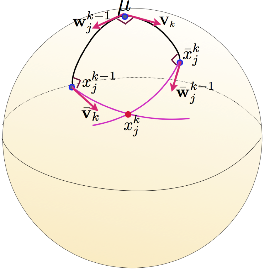
Figure 3: Approximation of $x_{j}$ from the first $k$ principal components.

Now, we will formulate a recursive scheme to reconstruct $x_{j}$. Let us reconstruct the data using the first $(k-1)$ principal components. Then, the $k^{th}$ approximated point $x_{j}^{k}$ is the intersection of two geodesics defined by $x_{j}^{k-1}$, $\bar{\mathbf{v}_{k}}$ and $\bar{x}_{j}^{k}$, $\bar{\mathbf{w}}_{j}^{k-1}$. Let these two great circles be denoted by

$$G_{1}(t)=\cos(t)x_{j}^{k-1}+\sin(t)\bar{\mathbf{v}_{k}}$$ (16)

$$G_{2}(u)=\cos(u)\bar{x}_{j}^{k}+\sin(u)\bar{\mathbf{w}}_{j}^{k-1}$$ (17)

At $t=\alpha_{1}$ and $u=\alpha_{2}$, let $G_{1}(\alpha_{1})=G_{2}(\alpha_{2})=x_{j}^{k}$. Since, $\bar{\mathbf{v}_{k}}$ and $\bar{\mathbf{w}}_{j}^{k-1}$ are mutually orthogonal, we get,

$$\tan(\alpha_{1})\tan(\alpha_{2})=<x_{j}^{k-1},\bar{\mathbf{w}}_{j}^{k-1}><\bar{x}_{j}^{k},\bar{\mathbf{v}_{k}}>$$ (18)

Note that, as our goal is to solve for $\alpha_{1}$ or $\alpha_{2}$ to get $x_{j}^{k}$, we need two equations. The second equation can be derived as follows:

$$d(\mu,G_{1}(\alpha_{1}))=d(\mu,G_{2}(\alpha_{2}))$$

This leads to,

$$\cos(\alpha_{2})=\frac{\cos(\alpha_{1})<\mu,x_{j}^{k-1}>}{<\mu,\bar{x}_{j}^{k}>}$$ (19)

Then, by solving Eqs. (18) and (19) we get,

$$a\cos^{4}(\alpha_{1})+b\cos^{2}(\alpha_{1})+d=0$$ (20)

where,

$$a=<\mu,x_{j}^{k-1}>^{2}<x_{j}^{k-1},\bar{\mathbf{w}}_{j}^{k-1}>^{2}<\bar{x}_{j}^{k},\bar{\mathbf{v}_{k}}>^{2}$$

$$-<\mu,x_{j}^{k-1}>^{2}$$

$$b=<\mu,\bar{x}_{j}^{k}>^{2}+<\mu,x_{j}^{k-1}>^{2}$$

and

$$d=-<\mu,\bar{x}_{j}^{k}>^{2}$$

By solving the equation (20), we get

$$\alpha_{1}=\arccos\bigg{(}\sqrt{\frac{-b+\sqrt{(b^{2}-4ad)}sgn(a)}{2a}}\bigg{)}$$ (21)

where, $sgn(.)$ is the signum function. Hence, $x_{j}^{k}=G_{1}(\alpha_{1})$. This completes the reconstruction algorithm. Our future efforts will be focused on using this reconstruction algorithm in a variety of applications mentioned earlier.

5 Conclusions

In this paper, we presented an efficient and accurate exact-PGA algorithm for (non-zero) constant curvature manifolds, namely the hypersphere $S^{n}$ and the hyperbolic space $H^{n}$. We presented analytic expressions for the shortest distance between the data point and the geodesic submanifolds, which is required in the PGA algorithm and in general involves solving a difficult optimization problem. Using these analytic expressions, we achieve a much more accurate and efficient solution for PGA on constant curvature manifolds, that are frequently encountered in Computer Vision, Medical Imaging and Machine Learning tasks. We presented comparison results on synthetic and real data sets demonstrating favorable performance of our algorithm in comparison to the state-of-the-art.

References

- [1] B. Afsari. Riemannian L^p center of mass: Existence, uniqueness, and convexity. Proceedings of the American Mathematical Society, 139(2):655–673, 2011.
- [2] S.-i. Amari and H. Nagaoka. Methods of information geometry, volume 191. American Mathematical Soc., 2007.
- [3] I. Bogdanova, X. Bresson, J.-P. Thiran, and P. Vandergheynst. Scale space analysis and active contours for omnidirectional images. Image Processing, IEEE Transactions on, 16(7):1888–1901, 2007.
- [4] W. M. Boothby. An introduction to differentiable manifolds and Riemannian geometry, volume 120. Academic press, 1986.
- [5] P. Brodatz. Textures: a photographic album for artists and designers. Dover Pubns, 1966.
- [6] S. I. Costa, S. A. Santos, and J. E. Strapasson. Fisher information distance: a geometrical reading. Discrete Applied Mathematics, 2014.
- [7] Y. Deng, A. Rangarajan, S. Eisenschenk, and B. C. Vemuri. A riemannian framework for matching point clouds represented by the schrödinger distance transform. In Computer Vision and Pattern Recognition (CVPR), 2014 IEEE Conference on, pages 3756–3761. IEEE, 2014.
- [8] P. T. Fletcher, C. Lu, S. M. Pizer, and S. Joshi. Principal geodesic analysis for the study of nonlinear statistics of shape. Medical Imaging, IEEE Transactions on, 23(8):995–1005, 2004.
- [9] M. Fréchet. Les éléments aléatoires de nature quelconque dans un espace distancié. In Annales de l’institut Henri Poincaré, volume 10, pages 215–310. Presses universitaires de France, 1948.
- [10] R. Hartley, J. Trumpf, Y. Dai, and H. Li. Rotation averaging. International journal of computer vision, 103(3):267–305, 2013.
- [11] J. Ho, Y. Xie, and B. Vemuri. On a nonlinear generalization of sparse coding and dictionary learning. In Proceedings of The 30th International Conference on Machine Learning, pages 1480–1488, 2013.
- [12] S. Huckemann, T. Hotz, and A. Munk. Intrinsic shape analysis: Geodesic pca for riemannian manifolds modulo isometric lie group actions. Statistica Sinica, 2010.
- [13] S. Huckemann and H. Ziezold. Principal component analysis for riemannian manifolds, with an application to triangular shape spaces. Advances in Applied Probability, pages 299–319, 2006.
- [14] B. Iversen. Hyperbolic geometry, volume 25. Cambridge University Press, 1992.
- [15] B. Jian and B. C. Vemuri. Metric learning using iwasawa decomposition. In Computer Vision, 2007. ICCV 2007. IEEE 11th International Conference on, pages 1–6. IEEE, 2007.
- [16] I. Jolliffe. Principal component analysis. Wiley Online Library, 2002.
- [17] E. L. Lehmann and G. Casella. Theory of point estimation, volume 31. Springer Science & Business Media, 1998.
- [18] R. Lenz, P. L. Carmona, and P. Meer. The hyperbolic geometry of illumination-induced chromaticity changes. In Computer Vision and Pattern Recognition, 2007. CVPR’07. IEEE Conference on, pages 1–6. IEEE, 2007.
- [19] R. Lenz and G. Granlund. If i had a fisheye i would not need so (1, n), or is hyperbolic geometry useful in image processing. In Proc. of the SSAB Symposium, Uppsala, Sweden, pages 49–52, 1998.
- [20] K. Mardia and I. Dryden. Shape distributions for landmark data. Advances in Applied Probability, pages 742–755, 1989.
- [21] A. Rangarajan. https://www.cise.ufl.edu/~anand/publications.html.
- [22] S. Said, N. Courty, N. Le Bihan, and S. J. Sangwine. Exact principal geodesic analysis for data on so (3). In 15th European Signal Processing Conference (EUSIPCO-2007), pages 1700–1705. EURASIP, 2007.
- [23] S. Sommer. https://github.com/nefan/smanifold, 2014.
- [24] S. Sommer, F. Lauze, S. Hauberg, and M. Nielsen. Manifold valued statistics, exact principal geodesic analysis and the effect of linear approximations. In Computer Vision–ECCV 2010, pages 43–56. Springer, 2010.
- [25] A. Terras. Harmonic analysis on symmetric spaces and applications. Springer, 1985.
- [26] M. E. Tipping and C. M. Bishop. Probabilistic principal component analysis. Journal of the Royal Statistical Society: Series B (Statistical Methodology), 61(3):611–622, 1999.
- [27] G. Uhlmann. Inverse Problems and Applications: Inside Out II, volume 60. Cambridge University Press, 2013.
- [28] Y. Wang, W. Dai, X. Gu, T. F. Chan, S.-T. Yau, A. W. Toga, and P. M. Thompson. Teichmüller shape space theory and its application to brain morphometry. In Medical Image Computing and Computer-Assisted Intervention–MICCAI 2009, pages 133–140. Springer, 2009.
- [29] W. Zeng, D. Samaras, and X. D. Gu. Ricci flow for 3d shape analysis. Pattern Analysis and Machine Intelligence, IEEE Transactions on, 32(4):662–677, 2010.
- [30] M. Zhang and P. T. Fletcher. Probabilistic principal geodesic analysis. In Advances in Neural Information Processing Systems, pages 1178–1186, 2013.