\corrauth

Heejin Ahn, Department of Mechanical Engineering, Massachusetts Institute of Technology, 77 Massachusetts Avenue, Cambridge, MA 02139, USA.

Robust Supervisors for Intersection Collision Avoidance in the Presence of Uncontrolled Vehicles

Heejin Ahn11affiliationmark:    Andrea Rizzi22affiliationmark:    Alessandro Colombo33affiliationmark:    and Domitilla Del Vecchio11affiliationmark: 11affiliationmark: Department of Mechanical Engineering, Massachusetts Institute of Technology, Cambridge, MA, USA
22affiliationmark: Tri-Institutional Program in Computational Biology and Medicine, Weill Cornell Medical College, New York, NY, USA
33affiliationmark: Dipartimento di Elettronica Informazione e Bioingegneria, Politecnico di Milano, Milano, Italy
hjahn@mit.edu
Abstract

We present the design and validation of a centralized controller, called a supervisor, for collision avoidance of multiple human-driven vehicles at a road intersection, considering measurement errors, unmodeled dynamics, and uncontrolled vehicles. We design the supervisor to be least restrictive, that is, to minimize its interferences with human drivers. This performance metric is given a precise mathematical form by splitting the design process into two subproblems: verification problem and supervisor-design problem. The verification problem determines whether an input signal exists that makes controlled vehicles avoid collisions at all future times. The supervisor is designed such that if the verification problem returns yes, it allows the drivers’ desired inputs; otherwise, it overrides controlled vehicles to prevent collisions. As a result, we propose exact and efficient supervisors. The exact supervisor solves the verification problem exactly but with combinatorial complexity. In contrast, the efficient supervisor solves the verification problem within a quantified approximation bound in polynomially bounded time with the number of controlled vehicles. We validate the performances of both supervisors through simulation and experimental testing.

keywords:
Class file, , SAGE Publications

1 Introduction

Autonomous robots have drawn attention in various applications, such as exploring unknown environment (Maimone et al. (2007)), moving materials in warehouses (Wurman et al. (2008)), and collecting data on ocean conditions (Smith et al. (2010)). Recently, there has been extensive research on autonomous vehicles from academic, industrial, and governmental sectors for the purpose of reducing the number of traffic accidents. Research has focused on developing fully autonomous vehicles as well as improving safety of human-driven vehicles by means of newly available automation, sensing, and communication capabilities. A major obstacle to the development of collision avoidance architecture for large traffic networks is computational complexity.

In general, there have been several approaches to reduce computational complexity in collision avoidance for multiple vehicles. In a decentralized framework, each vehicle makes its own decision to avoid collisions with its neighboring vehicles, thereby dividing a large problem into smaller local problems. To design a decentralized control law, Hoffmann and Tomlin (2008) and Gillula et al. (2011) used reachability analysis for hybrid systems, and Mastellone et al. (2008) defined a potential function. While computationally efficient, this framework is usually more conservative and unable to prevent a deadlock, where no further control input exists to terminate processes (Cassandras and Lafortune (2008)). A centralized framework considers a whole system and thus can be less conservative, but computationally demanding. Collision avoidance problems were formulated into mixed integer linear programming (MILP) by assuming discrete-time linear vehicle dynamic models (Richards et al. (2002); Borrelli et al. (2006)) and considering geometric construction of collisions with vehicle models of instantaneous speed or angle changes (Pallottino et al. (2002); Alonso-Ayuso et al. (2011)). These MILP formulations are then solved by commercially available software. In this paper, we present a centralized controller, in which the collision avoidance problem is translated into a scheduling problem and then solved by solving this scheduling problem. Moreover, we provide an approximate solution of this problem.

In collision avoidance problems at road intersections, the complexity can be mitigated to some extent by exploiting the fact that vehicles follow predefined paths, and side-impacts can be avoided by approximately scheduling their time of occupancy of the shared intersection (Peng and Akella (2005a, b)). Based on this concept, several autonomous intersection management schemes have been studied. Kowshik et al. (2011) proposed a hybrid architecture comprising an interplay between centralized coordination and distributed agents. Centralized coordination assigns time slots to agents, and distributed agents determine if they can cross an intersection within allocated time slots while avoiding rear-end collisions. Wu et al. (2012) employed an ant colony algorithm as an approximate solution for finding an optimal sequences of vehicles to improve traffic efficiency. Collision avoidance problems were formulated into nonlinear constrained optimization to eliminate overlaps of given trajectories inside an intersection (Lee and Park (2012)) and to minimize the risk of collision (Kamal et al. (2014)). These works consider fully autonomous vehicles and can solve collision avoidance problems by finding one safe input. However, when human operators drive vehicles, a controller needs to be least-restrictive, that is, override human drivers only when they can cause a collision.

To ensure least restrictiveness, all possible inputs must be taken into account, usually at expense of computational cost. Moreover, this exhaustive evaluation must be done frequently because controllers must keep monitoring vehicles’ safety and intervene only when drivers are unable to prevent collisions. In Hafner and Del Vecchio (2011); Hafner et al. (2013), a safety control was designed for two vehicles. Their controller was validated in laboratory experiments (Hafner and Del Vecchio (2011)) and field experiments (Hafner et al. (2013)). Colombo and Del Vecchio (2012) translated a collision detection problem to a scheduling problem and employed a scheduling algorithm to design a safety control for multiple vehicles. Rear-end collisions as well as intersection collisions were considered in Colombo and Del Vecchio (2014).

In this paper, we propose a least-restrictive controller, called a supervisor, that prevents intersection collisions among human-driven vehicles. Our work extends the result of Colombo and Del Vecchio (2012) in that 1) we consider sources of uncertainty, including measurement errors, unmodeled dynamics, and uncontrolled vehicles, and 2) we perform a lab-based experiment to validate the supervisor in a setting subject to many sources of uncertainty. Here, controlled vehicles communicate with and are controlled by the supervisor, whereas uncontrolled vehicles are not. The inclusion of uncontrolled vehicles accounts for a realistic mixed-traffic scenario where unequipped vehicles still travel on roads.

To design a supervisor, we formulate two problems: verification problem and supervisor-design problem. The verification problem determines the existence of an input signal that makes controlled vehicles avoid all future collisions. We prove that this problem is equivalent to an Inserted Idle-Time (IIT) scheduling problem, where an inserted idle-time represents a set of time intervals during which uncontrolled vehicles can occupy the intersection. This formulation was introduced in Ahn et al. (2014) to account for uncontrolled vehicles under perfect measurement and dynamic models. The supervisor is designed to override the drivers of controlled vehicles only when the verification problem determines that there will be no input signal to avoid collisions.

In order to study the trade-off between exactness and computational efficiency, we propose exact and efficient supervisors. The exact supervisor solves the verification problem exactly, and thus, overrides drivers only when strictly necessary. However, since the verification problem has combinatorial complexity, this supervisor is not scalable with the number of controlled vehicles. To improve the computational efficiency, the efficient supervisor is designed to solve the verification problem within a quantified approximation bound in polynomially bounded time. We validate the supervisors by performing computer simulations and lab-based experimental testing. Some of these experimental results were presented in Ahn et al. (2015).

This paper is organized as follows. In Section 2, we define an intersection model and a vehicle dynamic model. In Section 3, we formulate two problems: verification problem and supervisor-design problem, which are solved exactly in Section 4 and approximately in Section 5. The simulation results are given in Section 6, and the experimental results in Section 7.

2 System Definition

In this section, we introduce an intersection model and the vehicle dynamics.

2.1 Intersection model
Refer to caption
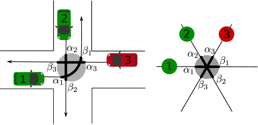
Figure 1: Road intersection (left) and its simplified model (right). We assume that the vehicles follow the prescribed paths, which intersect at one point. An intersection is modeled as an area containing this point (the shaded area), and its location is denoted by an open interval (αi,βi)subscript𝛼𝑖subscript𝛽𝑖(\alpha_{i},\beta_{i}) along the path of vehicle i𝑖i.

Consider n𝑛n human-driven vehicles approaching an intersection along n𝑛n different paths. As shown in Figure 1, the intersection is modeled as an area containing the points at which these paths intersect. An open interval (αi,βi)subscript𝛼𝑖subscript𝛽𝑖(\alpha_{i},\beta_{i})\subset\mathbb{R} denotes the location of this conflict area on the longitudinal path of vehicle i𝑖i. Among n𝑛n vehicles, ncsubscript𝑛𝑐n_{c} vehicles are communicating with a supervisor, which takes control of these vehicles when potential crashes are detected and returns control back to the drivers when there is no more threat. The other nc¯=nncsubscript𝑛¯𝑐𝑛subscript𝑛𝑐n_{\bar{c}}=n-n_{c} vehicles are not communicating with, and can never be controlled by the supervisor. The supervisor however can measure their positions and speeds and use these measurements to predict their possible future behaviors. We define a controlled set 𝒞𝒞\mathcal{C} as a set of controlled vehicles and an uncontrolled set 𝒞¯¯𝒞\bar{\mathcal{C}} as a set of uncontrolled vehicles. For notational simplicity, we number the vehicles such that 𝒞={1,2,,nc}𝒞12subscript𝑛𝑐\mathcal{C}=\{1,2,\ldots,n_{c}\} and 𝒞¯={nc+1,nc+2,,n}¯𝒞subscript𝑛𝑐1subscript𝑛𝑐2𝑛\bar{\mathcal{C}}=\{n_{c}+1,n_{c}+2,\ldots,n\}.

2.2 Vehicle model

To describe the longitudinal dynamics of vehicle i𝒞𝒞¯𝑖𝒞¯𝒞i\in\mathcal{C}\cup\bar{\mathcal{C}}, we introduce a state xi(t)=(yi(t),vi(t))Xi2subscript𝑥𝑖𝑡subscript𝑦𝑖𝑡subscript𝑣𝑖𝑡subscript𝑋𝑖superscript2x_{i}(t)=(y_{i}(t),v_{i}(t))\in X_{i}\subset\mathbb{R}^{2}, where yi(t)Yisubscript𝑦𝑖𝑡subscript𝑌𝑖y_{i}(t)\in Y_{i}\subseteq\mathbb{R} and vi(t)[vi,min,vi,max]subscript𝑣𝑖𝑡subscript𝑣𝑖𝑚𝑖𝑛subscript𝑣𝑖𝑚𝑎𝑥v_{i}(t)\in[v_{i,min},v_{i,max}]\subset\mathbb{R} are the position and the speed along the longitudinal path. Let di(t)=(dy,i(t),dv,i(t))2subscript𝑑𝑖𝑡subscript𝑑𝑦𝑖𝑡subscript𝑑𝑣𝑖𝑡superscript2d_{i}(t)=(d_{y,i}(t),d_{v,i}(t))\in\mathbb{R}^{2} denote a disturbance, where dy,i(t)[dy,i,min,dy,i,max]subscript𝑑𝑦𝑖𝑡subscript𝑑𝑦𝑖𝑚𝑖𝑛subscript𝑑𝑦𝑖𝑚𝑎𝑥d_{y,i}(t)\in[d_{y,i,min},d_{y,i,max}] and dv,i(t)[dv,i,min,dv,i,max]subscript𝑑𝑣𝑖𝑡subscript𝑑𝑣𝑖𝑚𝑖𝑛subscript𝑑𝑣𝑖𝑚𝑎𝑥d_{v,i}(t)\in[d_{v,i,min},d_{v,i,max}] account for unmodeled dynamics of yi(t)subscript𝑦𝑖𝑡y_{i}(t) and vi(t)subscript𝑣𝑖𝑡v_{i}(t), respectively. The longitudinal dynamics of controlled vehicle j𝒞𝑗𝒞j\in\mathcal{C} and uncontrolled vehicle γ𝒞¯𝛾¯𝒞\gamma\in\bar{\mathcal{C}} are modeled as

x˙j=Fj(xj,uj,dj),subscript˙𝑥𝑗subscript𝐹𝑗subscript𝑥𝑗subscript𝑢𝑗subscript𝑑𝑗\displaystyle\dot{x}_{j}=F_{j}(x_{j},u_{j},d_{j}), x˙γ=Fγ(xγ,wγ,dγ),subscript˙𝑥𝛾subscript𝐹𝛾subscript𝑥𝛾subscript𝑤𝛾subscript𝑑𝛾\displaystyle\dot{x}_{\gamma}=F_{\gamma}(x_{\gamma},w_{\gamma},d_{\gamma}), (1)

where ujUj:=[uj,min,uj,max]subscript𝑢𝑗subscript𝑈𝑗assignsubscript𝑢𝑗𝑚𝑖𝑛subscript𝑢𝑗𝑚𝑎𝑥u_{j}\in U_{j}:=[u_{j,min},u_{j,max}]\subset\mathbb{R} is a throttle or brake input to controlled vehicle j𝑗j applied by a supervisor, and wγ[wγ,min,wγ,max]subscript𝑤𝛾subscript𝑤𝛾𝑚𝑖𝑛subscript𝑤𝛾𝑚𝑎𝑥w_{\gamma}\in[w_{\gamma,min},w_{\gamma,max}]\subset\mathbb{R} is a driver-input to uncontrolled vehicle γ𝛾\gamma.

The parallel composition of (1) is denoted as follows:

𝐱˙=𝐅(𝐱,𝐮,𝐰,𝐝),˙𝐱𝐅𝐱𝐮𝐰𝐝\dot{\mathbf{x}}=\mathbf{F(x,u,w,d)},

where 𝐱=(x1,,xnc,xnc+1,,xn)𝐗𝐱subscript𝑥1subscript𝑥subscript𝑛𝑐subscript𝑥subscript𝑛𝑐1subscript𝑥𝑛𝐗\mathbf{x}=(x_{1},\ldots,x_{n_{c}},x_{n_{c}+1},\ldots,x_{n})\in\mathbf{X}, 𝐮=(u1,u2,,unc)𝐔𝐮subscript𝑢1subscript𝑢2subscript𝑢subscript𝑛𝑐𝐔\mathbf{u}=(u_{1},u_{2},\ldots,u_{n_{c}})\in\mathbf{U}, 𝐰=(wnc+1,wnc+2,,wn)𝐰subscript𝑤subscript𝑛𝑐1subscript𝑤subscript𝑛𝑐2subscript𝑤𝑛\mathbf{w}=(w_{n_{c}+1},w_{n_{c}+2},\ldots,w_{n}), and 𝐝=(d1,,dnc,dnc+1,,dn)𝐝subscript𝑑1subscript𝑑subscript𝑛𝑐subscript𝑑subscript𝑛𝑐1subscript𝑑𝑛\mathbf{d}=(d_{1},\ldots,d_{n_{c}},d_{n_{c}+1},\ldots,d_{n}). The output of the system is the position of all vehicles, denoted by 𝐲=(y1,,ync,ync+1,,yn)𝐘𝐲subscript𝑦1subscript𝑦subscript𝑛𝑐subscript𝑦subscript𝑛𝑐1subscript𝑦𝑛𝐘\mathbf{y}=(y_{1},\ldots,y_{n_{c}},y_{n_{c}+1},\ldots,y_{n})\in\mathbf{Y}.

Let uj()𝒰jsubscript𝑢𝑗subscript𝒰𝑗{u}_{j}(\cdot)\in\mathcal{U}_{j} and wγ()𝒲γsubscript𝑤𝛾subscript𝒲𝛾{w}_{\gamma}(\cdot)\in\mathcal{W}_{\gamma} denote an input signal to controlled vehicle j𝒞𝑗𝒞j\in\mathcal{C} and a driver-input signal to uncontrolled vehicle γ𝒞¯𝛾¯𝒞\gamma\in\bar{\mathcal{C}}, respectively. Let di()=(dy,i(),dv,i())𝒟isubscript𝑑𝑖subscript𝑑𝑦𝑖subscript𝑑𝑣𝑖subscript𝒟𝑖{d}_{i}(\cdot)=({d}_{y,i}(\cdot),{d}_{v,i}(\cdot))\in\mathcal{D}_{i} denote a disturbance signal of vehicle i𝒞𝒞¯𝑖𝒞¯𝒞i\in\mathcal{C}\cup\bar{\mathcal{C}}. We say uj()uj()subscript𝑢𝑗subscriptsuperscript𝑢𝑗{u}_{j}(\cdot)\leq u^{\prime}_{j}(\cdot) if uj(t)uj(t)subscript𝑢𝑗𝑡subscriptsuperscript𝑢𝑗𝑡u_{j}(t)\leq u^{\prime}_{j}(t) for all t𝑡t. Similarly, wγ()wγ()subscript𝑤𝛾subscriptsuperscript𝑤𝛾{w}_{\gamma}(\cdot)\leq w^{\prime}_{\gamma}(\cdot) if wγ(t)wγ(t)subscript𝑤𝛾𝑡subscriptsuperscript𝑤𝛾𝑡w_{\gamma}(t)\leq w^{\prime}_{\gamma}(t) for all t𝑡t, and di()di()subscript𝑑𝑖subscriptsuperscript𝑑𝑖{d}_{i}(\cdot)\leq d^{\prime}_{i}(\cdot) if dy,i(t)dy,i(t)subscript𝑑𝑦𝑖𝑡subscriptsuperscript𝑑𝑦𝑖𝑡d_{y,i}(t)\leq d^{\prime}_{y,i}(t) and dv,i(t)dv,i(t)subscript𝑑𝑣𝑖𝑡subscriptsuperscript𝑑𝑣𝑖𝑡d_{v,i}(t)\leq d^{\prime}_{v,i}(t) for all t𝑡t.

Let xj(t,uj(),dj(),xj(0))subscript𝑥𝑗𝑡subscript𝑢𝑗subscript𝑑𝑗subscript𝑥𝑗0x_{j}({t},{u}_{j}(\cdot),{d}_{j}(\cdot),x_{j}(0)) denote the state of controlled vehicle j𝑗j at time t𝑡t with an input signal uj()subscript𝑢𝑗{u}_{j}(\cdot) and a disturbance signal dj()subscript𝑑𝑗{d}_{j}(\cdot) starting at an initial state xj(0)subscript𝑥𝑗0x_{j}(0). Similarly, let xγ(t,wγ(),dγ(),xγ(0))subscript𝑥𝛾𝑡subscript𝑤𝛾subscript𝑑𝛾subscript𝑥𝛾0x_{\gamma}(t,{w}_{\gamma}(\cdot),{d}_{\gamma}(\cdot),x_{\gamma}(0)) denote the state of uncontrolled vehicle γ𝛾\gamma at time t𝑡t with a driver-input signal wγ()subscript𝑤𝛾{w}_{\gamma}(\cdot) and a disturbance signal dγ()subscript𝑑𝛾{d}_{\gamma}(\cdot) starting at xγ(0)subscript𝑥𝛾0x_{\gamma}(0). Unless the input signals and initial state are important, we write xi(t)subscript𝑥𝑖𝑡x_{i}(t) and xγ(t)subscript𝑥𝛾𝑡x_{\gamma}(t). We say xi(t)xi(t)subscript𝑥𝑖𝑡subscriptsuperscript𝑥𝑖𝑡x_{i}(t)\leq x^{\prime}_{i}(t) if yi(t)yi(t)subscript𝑦𝑖𝑡subscriptsuperscript𝑦𝑖𝑡y_{i}(t)\leq y^{\prime}_{i}(t) and vi(t)vi(t)subscript𝑣𝑖𝑡subscriptsuperscript𝑣𝑖𝑡v_{i}(t)\leq v^{\prime}_{i}(t) for all t𝑡t for i𝒞𝒞¯𝑖𝒞¯𝒞i\in\mathcal{C}\cup\bar{\mathcal{C}} and make the following assumptions.

Assumption 1.

The functions Fjsubscript𝐹𝑗F_{j} and Fγsubscript𝐹𝛾F_{\gamma} in (1) are order-preserving. That is, if uj()uj()subscript𝑢𝑗subscriptsuperscript𝑢𝑗{u}_{j}(\cdot)\leq u^{\prime}_{j}(\cdot), we have

xj(t,uj(),dj(),xj(0))xj(t,uj(),dj(),xj(0)).subscript𝑥𝑗𝑡subscript𝑢𝑗subscript𝑑𝑗subscript𝑥𝑗0subscript𝑥𝑗𝑡subscriptsuperscript𝑢𝑗subscript𝑑𝑗subscript𝑥𝑗0x_{j}({t},{u}_{j}(\cdot),{d}_{j}(\cdot),x_{j}(0))\leq x_{j}({t},u^{\prime}_{j}(\cdot),{d}_{j}(\cdot),x_{j}(0)).

Similarly, if dj()dj()subscript𝑑𝑗subscriptsuperscript𝑑𝑗{d}_{j}(\cdot)\leq d^{\prime}_{j}(\cdot), we have

xj(t,uj(),dj(),xj(0))xj(t,uj(),dj(),xj(0)).subscript𝑥𝑗𝑡subscript𝑢𝑗subscript𝑑𝑗subscript𝑥𝑗0subscript𝑥𝑗𝑡subscript𝑢𝑗subscriptsuperscript𝑑𝑗subscript𝑥𝑗0x_{j}({t},{u}_{j}(\cdot),{d}_{j}(\cdot),x_{j}(0))\leq x_{j}({t},{u}_{j}(\cdot),d^{\prime}_{j}(\cdot),x_{j}(0)).

Furthermore, if xj(0)xj(0)subscript𝑥𝑗0subscriptsuperscript𝑥𝑗0x_{j}(0)\leq x^{\prime}_{j}(0), we have

xj(t,uj(),dj(),xj(0))xj(t,uj(),dj(),xj(0)).subscript𝑥𝑗𝑡subscript𝑢𝑗subscript𝑑𝑗subscript𝑥𝑗0subscript𝑥𝑗𝑡subscript𝑢𝑗subscript𝑑𝑗subscriptsuperscript𝑥𝑗0x_{j}({t},{u}_{j}(\cdot),{d}_{j}(\cdot),x_{j}(0))\leq x_{j}({t},{u}_{j}(\cdot),{d}_{j}(\cdot),{x}^{\prime}_{j}(0)).

The same relations hold for the state of uncontrolled vehicle γ𝛾\gamma.

Assumption 2.

For all i𝒞𝒞¯𝑖𝒞¯𝒞i\in\mathcal{C}\cup\bar{\mathcal{C}}, y˙i(t)0subscript˙𝑦𝑖𝑡0\dot{y}_{i}(t)\geq 0 for all t𝑡t. Thus, the outputs yj(t,uj(),dj(),xj(0))subscript𝑦𝑗𝑡subscript𝑢𝑗subscript𝑑𝑗subscript𝑥𝑗0y_{j}({t},{u}_{j}(\cdot),{d}_{j}(\cdot),x_{j}(0)) and yγ(t,wγ(),dγ(),xγ(0))subscript𝑦𝛾𝑡subscript𝑤𝛾subscript𝑑𝛾subscript𝑥𝛾0y_{\gamma}(t,{w}_{\gamma}(\cdot),{d}_{\gamma}(\cdot),x_{\gamma}(0)) are non-decreasing in t𝑡t.

Assumption 3.

For all j𝒞𝑗𝒞j\in\mathcal{C}, xj(t,uj(),dj(),xj(0))subscript𝑥𝑗𝑡subscript𝑢𝑗subscript𝑑𝑗subscript𝑥𝑗0{x}_{j}(t,{u}_{j}(\cdot),{d}_{j}(\cdot),{x}_{j}(0)) is continuously dependent on uj()𝒰jsubscript𝑢𝑗subscript𝒰𝑗{u}_{j}(\cdot)\in\mathcal{U}_{j}, and the input signal space 𝒰jsubscript𝒰𝑗\mathcal{U}_{j} is path-connected.

Let 𝐱(t,𝐮(),𝐰(),𝐝(),𝐱(0))𝐱𝑡𝐮𝐰𝐝𝐱0\mathbf{x}(t,\mathbf{u}(\cdot),\mathbf{w}(\cdot),\mathbf{d}(\cdot),\mathbf{x}(0)) denote the aggregate state with 𝐮()𝒰,𝐰()𝒲formulae-sequence𝐮𝒰𝐰𝒲\mathbf{u}(\cdot)\in\mathcal{U},\mathbf{w}(\cdot)\in\mathcal{W}, and 𝐝()𝒟𝐝𝒟\mathbf{d}(\cdot)\in\mathcal{D}. This can also be written as 𝐱(t)𝐱𝑡\mathbf{x}(t) if the other arguments are not important.

Notice that the vehicle dynamics (1) are subject to uncertainty originated from disturbances djsubscript𝑑𝑗d_{j} and dγsubscript𝑑𝛾d_{\gamma} and an unknown driver-input wγsubscript𝑤𝛾w_{\gamma}. In addition to these, we consider a measurement noise δi:=(δy,i,δv,i)assignsubscript𝛿𝑖subscript𝛿𝑦𝑖subscript𝛿𝑣𝑖\delta_{i}:=(\delta_{y,i},\delta_{v,i}) for i𝒞𝒞¯𝑖𝒞¯𝒞i\in\mathcal{C}\cup\bar{\mathcal{C}}, where δy,isubscript𝛿𝑦𝑖\delta_{y,i}\in\mathbb{R} and δv,isubscript𝛿𝑣𝑖\delta_{v,i}\in\mathbb{R} are noises on the position measurement ym,i(t)subscript𝑦𝑚𝑖𝑡y_{m,i}(t) and the speed measurement vm,i(t)subscript𝑣𝑚𝑖𝑡v_{m,i}(t) at some time t𝑡t, respectively. Then, the actual state xi(t)=(yi(t),vi(t))subscript𝑥𝑖𝑡subscript𝑦𝑖𝑡subscript𝑣𝑖𝑡x_{i}(t)=(y_{i}(t),v_{i}(t)) satisfies the following equation:

yi(t)=ym,i(t)+δy,i,subscript𝑦𝑖𝑡subscript𝑦𝑚𝑖𝑡subscript𝛿𝑦𝑖\displaystyle y_{i}(t)=y_{m,i}(t)+\delta_{y,i}, vi(t)=vm,i(t)+δv,i.subscript𝑣𝑖𝑡subscript𝑣𝑚𝑖𝑡subscript𝛿𝑣𝑖\displaystyle v_{i}(t)=v_{m,i}(t)+\delta_{v,i}. (2)

Let xm,i(t)=(ym,i(t),vm,i(t))subscript𝑥𝑚𝑖𝑡subscript𝑦𝑚𝑖𝑡subscript𝑣𝑚𝑖𝑡x_{m,i}(t)=(y_{m,i}(t),v_{m,i}(t)) denote the state measurement. Then, (2) can be rewritten as xi(t)=xm,i(t)+δisubscript𝑥𝑖𝑡subscript𝑥𝑚𝑖𝑡subscript𝛿𝑖x_{i}(t)=x_{m,i}(t)+\delta_{i}. We make an assumption as follows.

Assumption 4.

The measurement noise is bounded, that is, δi[δi,min,δi,max]subscript𝛿𝑖subscript𝛿𝑖𝑚𝑖𝑛subscript𝛿𝑖𝑚𝑎𝑥\delta_{i}\in[\delta_{i,min},\delta_{i,max}].

The aggregate state measurement is denoted by 𝐱m(t)subscript𝐱𝑚𝑡\mathbf{x}_{m}(t), and then, 𝐱(t)=𝐱m(t)+δ𝐱𝑡subscript𝐱𝑚𝑡𝛿\mathbf{x}(t)=\mathbf{x}_{m}(t)+\delta, where δΔ:=[δmin,δmax]𝛿Δassignsubscript𝛿𝑚𝑖𝑛subscript𝛿𝑚𝑎𝑥\delta\in\Delta:=[\delta_{min},\delta_{max}] is the aggregated measurement noise.

2.3 The state estimation

We define a set of states [𝐱a(t),𝐱b(t)]superscript𝐱𝑎𝑡superscript𝐱𝑏𝑡[\mathbf{x}^{a}(t),\mathbf{x}^{b}(t)], called the state estimation, that provides a lower and upper bound of the exact state, that is, 𝐱(t)[𝐱a(t),𝐱b(t)]𝐱𝑡superscript𝐱𝑎𝑡superscript𝐱𝑏𝑡\mathbf{x}(t)\in[\mathbf{x}^{a}(t),\mathbf{x}^{b}(t)] for all t𝑡t. At t=0𝑡0t=0, the state estimation is defined as 𝐱a(0)=𝐱m(0)+δminsuperscript𝐱𝑎0subscript𝐱𝑚0subscript𝛿𝑚𝑖𝑛\mathbf{x}^{a}(0)=\mathbf{x}_{m}(0)+\delta_{min} and 𝐱b(0)=𝐱m(0)+δmaxsuperscript𝐱𝑏0subscript𝐱𝑚0subscript𝛿𝑚𝑎𝑥\mathbf{x}^{b}(0)=\mathbf{x}_{m}(0)+\delta_{max}, so that 𝐱(0)[𝐱a(0),𝐱b(0)]𝐱0superscript𝐱𝑎0superscript𝐱𝑏0\mathbf{x}(0)\in[\mathbf{x}^{a}(0),\mathbf{x}^{b}(0)] because of (2) and Assumption 4. Given the intial state estimation [𝐱a(0),𝐱b(0)]superscript𝐱𝑎0superscript𝐱𝑏0[\mathbf{x}^{a}(0),\mathbf{x}^{b}(0)] and an input signal 𝐮()𝐮\mathbf{u}(\cdot), the state estimation [𝐱a(t,𝐮(),𝐱a(0)),𝐱b(t,𝐮(),𝐱b(0))]superscript𝐱𝑎𝑡𝐮superscript𝐱𝑎0superscript𝐱𝑏𝑡𝐮superscript𝐱𝑏0[\mathbf{x}^{a}(t,\mathbf{u}(\cdot),\mathbf{x}^{a}(0)),\mathbf{x}^{b}(t,\mathbf{u}(\cdot),\mathbf{x}^{b}(0))] at time t𝑡t is defined as follows: for j𝒞𝑗𝒞j\in\mathcal{C},

xja(t,uj(),xja(0)):=mindj()𝒟j,xj(0)[xja(0),xjb(0)]xj(t,uj(),dj(),xj(0)),xjb(t,uj(),xjb(0)):=maxdj()𝒟j,xj(0)[xja(0),xjb(0)]xj(t,uj(),dj(),xj(0)).formulae-sequenceassignsubscriptsuperscript𝑥𝑎𝑗𝑡subscript𝑢𝑗superscriptsubscript𝑥𝑗𝑎0subscriptsubscript𝑑𝑗subscript𝒟𝑗subscript𝑥𝑗0absentsubscriptsuperscript𝑥𝑎𝑗0subscriptsuperscript𝑥𝑏𝑗0subscript𝑥𝑗𝑡subscript𝑢𝑗subscript𝑑𝑗subscript𝑥𝑗0assignsubscriptsuperscript𝑥𝑏𝑗𝑡subscript𝑢𝑗superscriptsubscript𝑥𝑗𝑏0subscriptsubscript𝑑𝑗subscript𝒟𝑗subscript𝑥𝑗0absentsubscriptsuperscript𝑥𝑎𝑗0subscriptsuperscript𝑥𝑏𝑗0subscript𝑥𝑗𝑡subscript𝑢𝑗subscript𝑑𝑗subscript𝑥𝑗0\displaystyle\begin{split}&x^{a}_{j}(t,{u}_{j}(\cdot),x_{j}^{a}(0)):=\min_{\begin{subarray}{\centering}{d}_{j}(\cdot)\in\mathcal{D}_{j},x_{j}(0)\\ \in[x^{a}_{j}(0),x^{b}_{j}(0)]\@add@centering\end{subarray}}x_{j}(t,{u}_{j}(\cdot),{d}_{j}(\cdot),x_{j}(0)),\\ &x^{b}_{j}(t,{u}_{j}(\cdot),x_{j}^{b}(0)):=\max_{\begin{subarray}{\centering}{d}_{j}(\cdot)\in\mathcal{D}_{j},x_{j}(0)\\ \in[x^{a}_{j}(0),x^{b}_{j}(0)]\@add@centering\end{subarray}}x_{j}(t,{u}_{j}(\cdot),{d}_{j}(\cdot),x_{j}(0)).\end{split} (3)

For γ𝒞¯,𝛾¯𝒞\gamma\in\bar{\mathcal{C}},

xγa(t):=minwγ()𝒲γ,dγ()𝒟γ,xγ(0)[xγa(0),xγb(0)]xγ(t,wγ(),dγ(),xγ(0)),xγb(t):=maxwγ()𝒲γ,dγ()𝒟γ,xγ(0)[xγa(0),xγb(0)]xγ(t,wγ(),dγ(),xγ(0)).formulae-sequenceassignsubscriptsuperscript𝑥𝑎𝛾𝑡subscriptformulae-sequencesubscript𝑤𝛾subscript𝒲𝛾subscript𝑑𝛾subscript𝒟𝛾subscript𝑥𝛾0subscriptsuperscript𝑥𝑎𝛾0subscriptsuperscript𝑥𝑏𝛾0subscript𝑥𝛾𝑡subscript𝑤𝛾subscript𝑑𝛾subscript𝑥𝛾0assignsubscriptsuperscript𝑥𝑏𝛾𝑡subscriptformulae-sequencesubscript𝑤𝛾subscript𝒲𝛾subscript𝑑𝛾subscript𝒟𝛾subscript𝑥𝛾0subscriptsuperscript𝑥𝑎𝛾0subscriptsuperscript𝑥𝑏𝛾0subscript𝑥𝛾𝑡subscript𝑤𝛾subscript𝑑𝛾subscript𝑥𝛾0\displaystyle\begin{split}&x^{a}_{\gamma}(t):=\min_{\begin{subarray}{\centering}{w}_{\gamma}(\cdot)\in\mathcal{W}_{\gamma},{d}_{\gamma}(\cdot)\in\mathcal{D}_{\gamma},\\ x_{\gamma}(0)\in[x^{a}_{\gamma}(0),x^{b}_{\gamma}(0)]\@add@centering\end{subarray}}x_{\gamma}(t,{w}_{\gamma}(\cdot),{d}_{\gamma}(\cdot),x_{\gamma}(0)),\\ &x^{b}_{\gamma}(t):=\max_{\begin{subarray}{\centering}{w}_{\gamma}(\cdot)\in\mathcal{W}_{\gamma},{d}_{\gamma}(\cdot)\in\mathcal{D}_{\gamma},\\ x_{\gamma}(0)\in[x^{a}_{\gamma}(0),x^{b}_{\gamma}(0)]\@add@centering\end{subarray}}x_{\gamma}(t,{w}_{\gamma}(\cdot),{d}_{\gamma}(\cdot),x_{\gamma}(0)).\end{split} (4)

The state estimation is denoted by [𝐱a(t,𝐮(),𝐱a(0)),𝐱b(t,𝐮(),𝐱b(0))]superscript𝐱𝑎𝑡𝐮superscript𝐱𝑎0superscript𝐱𝑏𝑡𝐮superscript𝐱𝑏0[\mathbf{x}^{a}(t,\mathbf{u}(\cdot),\mathbf{x}^{a}(0)),\mathbf{x}^{b}(t,\mathbf{u}(\cdot),\mathbf{x}^{b}(0))] or [𝐱a(t),𝐱b(t)]superscript𝐱𝑎𝑡superscript𝐱𝑏𝑡[\mathbf{x}^{a}(t),\mathbf{x}^{b}(t)] if the omitted arguments are not necessary.

By these definitions, the state estimation guarantees that given an initial state estimation [𝐱a(0),𝐱b(0)]superscript𝐱𝑎0superscript𝐱𝑏0[\mathbf{x}^{a}(0),\mathbf{x}^{b}(0)] and an input signal 𝐮()𝐮\mathbf{u}(\cdot),

𝐱(t,𝐮(),𝐰(),𝐝(),𝐱(0))[𝐱a(t,𝐮(),𝐱a(0)),𝐱b(t,𝐮(),𝐱b(0))],𝐱𝑡𝐮𝐰𝐝𝐱0superscript𝐱𝑎𝑡𝐮superscript𝐱𝑎0superscript𝐱𝑏𝑡𝐮superscript𝐱𝑏0\displaystyle\begin{split}\mathbf{x}(t,\mathbf{u}(\cdot),&\mathbf{w}(\cdot),\mathbf{d}(\cdot),\mathbf{x}(0))\\ &\in[\mathbf{x}^{a}(t,\mathbf{u}(\cdot),\mathbf{x}^{a}(0)),\mathbf{x}^{b}(t,\mathbf{u}(\cdot),\mathbf{x}^{b}(0))],\end{split} (5)

for all t𝑡t for any 𝐰()𝒲𝐰𝒲\mathbf{w}(\cdot)\in\mathcal{W} and 𝐝()𝒟𝐝𝒟\mathbf{d}(\cdot)\in\mathcal{D} for any 𝐱(0)[𝐱a(0),𝐱b(0)]𝐱0superscript𝐱𝑎0superscript𝐱𝑏0\mathbf{x}(0)\in[\mathbf{x}^{a}(0),\mathbf{x}^{b}(0)].

Notice that xja(t,uj(),xja(0))subscriptsuperscript𝑥𝑎𝑗𝑡subscript𝑢𝑗subscriptsuperscript𝑥𝑎𝑗0x^{a}_{j}(t,{u}_{j}(\cdot),x^{a}_{j}(0)) and xjb(t,uj(),xjb(0))subscriptsuperscript𝑥𝑏𝑗𝑡subscript𝑢𝑗superscriptsubscript𝑥𝑗𝑏0x^{b}_{j}(t,{u}_{j}(\cdot),x_{j}^{b}(0)) satisfy the inequalities in Assumption 1. We can define the position estimation, denoted by [𝐲a(t,𝐮(),𝐱a(0)),𝐲b(t,𝐮(),𝐱b(0)))][\mathbf{y}^{a}(t,\mathbf{u}(\cdot),\mathbf{x}^{a}(0)),\mathbf{y}^{b}(t,\mathbf{u}(\cdot),\mathbf{x}^{b}(0)))] by letting xia(t)=(yia(t),)subscriptsuperscript𝑥𝑎𝑖𝑡subscriptsuperscript𝑦𝑎𝑖𝑡x^{a}_{i}(t)=(y^{a}_{i}(t),\cdot) and xib(t)=(yib(t),)subscriptsuperscript𝑥𝑏𝑖𝑡subscriptsuperscript𝑦𝑏𝑖𝑡x^{b}_{i}(t)=(y^{b}_{i}(t),\cdot) for all i𝒞𝒞¯𝑖𝒞¯𝒞i\in\mathcal{C}\cup\bar{\mathcal{C}}. Throughout this paper, we use ‘\cdot’ in a vector if specifying the entry is not important. The position estimation also inherits the order-preserving property from 𝐲(t)𝐲𝑡\mathbf{y}(t). Later in Section 4.2, this estimation can be updated using the state measurement.

Refer to caption
Figure 2: 𝐮desirek,()subscriptsuperscript𝐮𝑘𝑑𝑒𝑠𝑖𝑟𝑒\mathbf{u}^{{k},\infty}_{desire}(\cdot) is an artificially constructed signal that equals to 𝐮desireksubscriptsuperscript𝐮𝑘𝑑𝑒𝑠𝑖𝑟𝑒\mathbf{u}^{k}_{desire} for time [kτ,(k+1)τ)𝑘𝜏𝑘1𝜏[k\tau,(k+1)\tau) as in (6). 𝐮safek,()subscriptsuperscript𝐮𝑘𝑠𝑎𝑓𝑒\mathbf{u}^{{k,\infty}}_{safe}(\cdot) is an safe input signal that makes the system avoid the Bad set as in (7).
Refer to caption
Figure 3: Illustration of the supervisor. At time kτ𝑘𝜏k\tau, the supervisor takes the desired input of controlled vehicles’ drivers 𝐮desireksubscriptsuperscript𝐮𝑘𝑑𝑒𝑠𝑖𝑟𝑒\mathbf{u}^{k}_{desire} and the state estimation [𝐱a(kτ),𝐱b(kτ)]superscript𝐱𝑎𝑘𝜏superscript𝐱𝑏𝑘𝜏[\mathbf{x}^{a}(k\tau),\mathbf{x}^{b}(k\tau)]. Depending on the existence of 𝐮desirek,()subscriptsuperscript𝐮𝑘𝑑𝑒𝑠𝑖𝑟𝑒\mathbf{u}^{{k},\infty}_{desire}(\cdot) that prevents all the vehicles from entering the Bad set for all t𝑡t for any 𝐰()𝒲,𝐝()𝒟,formulae-sequence𝐰𝒲𝐝𝒟\mathbf{w}(\cdot)\in\mathcal{W},\mathbf{d}(\cdot)\in\mathcal{D}, and 𝐱(kτ)[𝐱a(kτ),𝐱b(kτ)]𝐱𝑘𝜏superscript𝐱𝑎𝑘𝜏superscript𝐱𝑏𝑘𝜏\mathbf{x}(k\tau)\in[\mathbf{x}^{a}(k\tau),\mathbf{x}^{b}(k\tau)], the supervisor either allows the drivers to travel with their desired input 𝐮desirek()superscriptsubscript𝐮𝑑𝑒𝑠𝑖𝑟𝑒𝑘\mathbf{u}_{desire}^{k}(\cdot) or overrides them with the safe input 𝐮safek()superscriptsubscript𝐮𝑠𝑎𝑓𝑒𝑘\mathbf{u}_{safe}^{k}(\cdot).

3 Problem Statement

Let us define an intersection collision. Since an intersection is modeled as a single conflict area, we consider a collision occurs if at least two vehicles are simultaneously inside the intersection. The output configurations corresponding to collisions belong to the Bad set, denoted by BY𝐵𝑌B\subset Y. The Bad set is defined as follows:

B:={\displaystyle B:=\{ 𝐲Y:yi(αi,βi) and yj(αj,βj):𝐲𝑌subscript𝑦𝑖subscript𝛼𝑖subscript𝛽𝑖 and subscript𝑦𝑗subscript𝛼𝑗subscript𝛽𝑗\displaystyle\mathbf{y}\in Y:y_{i}\in(\alpha_{i},\beta_{i})\text{ and }y_{j}\in(\alpha_{j},\beta_{j})
for some ij such that i𝒞𝒞¯ and j𝒞}.\displaystyle\text{ for some }i\neq j\text{ such that }i\in\mathcal{C}\cup\bar{\mathcal{C}}\text{ and }j\in\mathcal{C}\}.

Throughout this paper, we assume that uncontrolled vehicles do not crash among themselves. This assumption enables us to focus on preventing collisions in which at least one controlled vehicle is involved.

A supervisor runs in discrete time with a time step τ𝜏\tau. At time kτ𝑘𝜏k\tau where k𝑘k is a nonnegative integer, a desired input 𝐮desirek𝐔superscriptsubscript𝐮𝑑𝑒𝑠𝑖𝑟𝑒𝑘𝐔\mathbf{u}_{desire}^{k}\in\mathbf{U} and a state 𝐱m(kτ)𝐗subscript𝐱𝑚𝑘𝜏𝐗\mathbf{x}_{m}(k\tau)\in\mathbf{X} are measured. Then, a state estimation [𝐱a(kτ),𝐱b(kτ)]superscript𝐱𝑎𝑘𝜏superscript𝐱𝑏𝑘𝜏[\mathbf{x}^{a}(k\tau),\mathbf{x}^{b}(k\tau)] is updated to satisfy 𝐱(kτ)[𝐱a(kτ),𝐱b(kτ)][𝐱m(kτ)+δmin,𝐱m(kτ)+δmax]𝐱𝑘𝜏superscript𝐱𝑎𝑘𝜏superscript𝐱𝑏𝑘𝜏subscript𝐱𝑚𝑘𝜏subscript𝛿𝑚𝑖𝑛subscript𝐱𝑚𝑘𝜏subscript𝛿𝑚𝑎𝑥\mathbf{x}(k\tau)\in[\mathbf{x}^{a}(k\tau),\mathbf{x}^{b}(k\tau)]\subseteq[\mathbf{x}_{m}(k\tau)+\delta_{min},\mathbf{x}_{m}(k\tau)+\delta_{max}]. The desired input 𝐮desireksuperscriptsubscript𝐮𝑑𝑒𝑠𝑖𝑟𝑒𝑘\mathbf{u}_{desire}^{k} is a vector of current inputs of controlled vehicles’ drivers at time kτ𝑘𝜏k\tau. As illustrated in Figure 2, we define desired input signals 𝐮desirek()𝒰superscriptsubscript𝐮𝑑𝑒𝑠𝑖𝑟𝑒𝑘𝒰\mathbf{u}_{desire}^{k}(\cdot)\in\mathcal{U} on time [kτ,(k+1)τ)𝑘𝜏𝑘1𝜏[k\tau,(k+1)\tau) and 𝐮desirek,()𝒰subscriptsuperscript𝐮𝑘𝑑𝑒𝑠𝑖𝑟𝑒𝒰\mathbf{u}^{{k},\infty}_{desire}(\cdot)\in\mathcal{U} on time [kτ,)𝑘𝜏[k\tau,\infty) such that

𝐮desirek(t)=𝐮desirek,(t)=𝐮desirekfort[kτ,(k+1)τ).superscriptsubscript𝐮𝑑𝑒𝑠𝑖𝑟𝑒𝑘𝑡subscriptsuperscript𝐮𝑘𝑑𝑒𝑠𝑖𝑟𝑒𝑡superscriptsubscript𝐮𝑑𝑒𝑠𝑖𝑟𝑒𝑘for𝑡𝑘𝜏𝑘1𝜏\mathbf{u}_{desire}^{k}(t)=\mathbf{u}^{k,\infty}_{desire}(t)=\mathbf{u}_{desire}^{k}~{}\text{for}~{}t\in[k\tau,(k+1)\tau). (6)

Also, we define a safe input signal 𝐮safek,()subscriptsuperscript𝐮𝑘𝑠𝑎𝑓𝑒\mathbf{u}^{{k,\infty}}_{safe}(\cdot) on time [kτ,)𝑘𝜏[k\tau,\infty) such that

𝐰()𝒲,𝐝()𝒟,𝐱(kτ)[𝐱a(kτ),𝐱b(kτ)],𝐲(t,𝐮safek,(),𝐰(),𝐝(),𝐱(kτ))Bfor allt.formulae-sequencefor-all𝐰𝒲formulae-sequence𝐝𝒟formulae-sequence𝐱𝑘𝜏superscript𝐱𝑎𝑘𝜏superscript𝐱𝑏𝑘𝜏𝐲𝑡subscriptsuperscript𝐮𝑘𝑠𝑎𝑓𝑒𝐰𝐝𝐱𝑘𝜏𝐵for all𝑡\displaystyle\begin{split}\forall&\mathbf{w}(\cdot)\in\mathcal{W},\mathbf{d}(\cdot)\in\mathcal{D},\mathbf{x}(k\tau)\in[\mathbf{x}^{a}(k\tau),\mathbf{x}^{b}(k\tau)],\\ &\mathbf{y}(t,\mathbf{u}^{{k,\infty}}_{safe}(\cdot),\mathbf{w}(\cdot),\mathbf{d}(\cdot),\mathbf{x}(k\tau))\notin B~{}\text{for all}~{}t.\end{split} (7)

Let 𝐮safek()subscriptsuperscript𝐮𝑘𝑠𝑎𝑓𝑒\mathbf{u}^{{k}}_{safe}(\cdot) be 𝐮safek,()subscriptsuperscript𝐮𝑘𝑠𝑎𝑓𝑒\mathbf{u}^{{k,\infty}}_{safe}(\cdot) restricted to time [kτ,(k+1)τ)𝑘𝜏𝑘1𝜏[k\tau,(k+1)\tau).

The supervisor s([𝐱a(kτ),𝐱b(kτ)],𝐮desirek)𝑠superscript𝐱𝑎𝑘𝜏superscript𝐱𝑏𝑘𝜏superscriptsubscript𝐮𝑑𝑒𝑠𝑖𝑟𝑒𝑘s([\mathbf{x}^{a}(k\tau),\mathbf{x}^{b}(k\tau)],\mathbf{u}_{desire}^{k}) is designed according to the following problem, which is illustrated in Figure 3.

Problem 1 ((Supervisor-design)).

Design a supervisor s([𝐱a(kτ),𝐱b(kτ)],𝐮desirek)𝑠superscript𝐱𝑎𝑘𝜏superscript𝐱𝑏𝑘𝜏superscriptsubscript𝐮𝑑𝑒𝑠𝑖𝑟𝑒𝑘s([\mathbf{x}^{a}(k\tau),\mathbf{x}^{b}(k\tau)],\mathbf{u}_{desire}^{k}) such that for any 𝐰(),𝐝(),𝐰𝐝\mathbf{w}(\cdot),\mathbf{d}(\cdot), and 𝐱(kτ)[𝐱a(kτ),𝐱b(kτ)]𝐱𝑘𝜏superscript𝐱𝑎𝑘𝜏superscript𝐱𝑏𝑘𝜏\mathbf{x}(k\tau)\in[\mathbf{x}^{a}(k\tau),\mathbf{x}^{b}(k\tau)], it returns

{𝐮desirek()if𝐮desirek,(): for allt0𝐲(t,𝐮desirek,(),𝐰(),𝐝(),𝐱(kτ))B𝐮safek()otherwise,casessuperscriptsubscript𝐮𝑑𝑒𝑠𝑖𝑟𝑒𝑘:ifsubscriptsuperscript𝐮𝑘𝑑𝑒𝑠𝑖𝑟𝑒 for all𝑡0otherwise𝐲𝑡subscriptsuperscript𝐮𝑘𝑑𝑒𝑠𝑖𝑟𝑒𝐰𝐝𝐱𝑘𝜏𝐵subscriptsuperscript𝐮𝑘𝑠𝑎𝑓𝑒otherwise,\begin{cases}\mathbf{u}_{desire}^{k}(\cdot)&\text{if}~{}\exists\mathbf{u}^{{k},\infty}_{desire}(\cdot):\text{ for all}~{}t\geq 0\\ &\mathbf{y}(t,\mathbf{u}^{{k},\infty}_{desire}(\cdot),\mathbf{w}(\cdot),\mathbf{d}(\cdot),\mathbf{x}(k\tau))\notin B\\ \mathbf{u}^{{k}}_{safe}(\cdot)&\text{otherwise,}\end{cases}

and it is non-blocking, that is, if s([𝐱a((k1)τ),𝐱b((k1)τ)],𝐮desirek1)𝑠superscript𝐱𝑎𝑘1𝜏superscript𝐱𝑏𝑘1𝜏superscriptsubscript𝐮𝑑𝑒𝑠𝑖𝑟𝑒𝑘1s([\mathbf{x}^{a}((k-1)\tau),\mathbf{x}^{b}((k-1)\tau)],\mathbf{u}_{desire}^{k-1})\neq\emptyset, then for any 𝐮desirek𝐔,superscriptsubscript𝐮𝑑𝑒𝑠𝑖𝑟𝑒𝑘𝐔\mathbf{u}_{desire}^{k}\in\mathbf{U}, we have s([𝐱a(kτ),𝐱b(kτ)],𝐮desirek).𝑠superscript𝐱𝑎𝑘𝜏superscript𝐱𝑏𝑘𝜏superscriptsubscript𝐮𝑑𝑒𝑠𝑖𝑟𝑒𝑘s([\mathbf{x}^{a}(k\tau),\mathbf{x}^{b}(k\tau)],\mathbf{u}_{desire}^{k})\neq\emptyset.

The supervisor in Problem 1 is least restrictive in the sense that overrides are activated only when the desired input of controlled vehicles’ drivers would lead to collisions at some future times. To distinguish between safe and unsafe inputs, the supervisor needs to verify that the state reached using the desired input is compatible with a safe evolution of the system. This introduces the following problem.

Problem 2 ((Verification)).

Given an initial state estimation [𝐱a(0),𝐱b(0)]superscript𝐱𝑎0superscript𝐱𝑏0[\mathbf{x}^{a}(0),\mathbf{x}^{b}(0)], determine if there exists an input signal 𝐮()𝐮\mathbf{u}(\cdot) that guarantees 𝐲(t,𝐮(),𝐰(),𝐝(),𝐱(0))B𝐲𝑡𝐮𝐰𝐝𝐱0𝐵\mathbf{y}(t,\mathbf{u}(\cdot),\mathbf{w}(\cdot),\mathbf{d}(\cdot),\mathbf{x}(0))\notin B for all t0𝑡0t\geq 0 for any 𝐰()𝒲,𝐝()𝒟,formulae-sequence𝐰𝒲𝐝𝒟\mathbf{w}(\cdot)\in\mathcal{W},\mathbf{d}(\cdot)\in\mathcal{D}, and 𝐱(0)[𝐱a(0),𝐱b(0)]𝐱0superscript𝐱𝑎0superscript𝐱𝑏0\mathbf{x}(0)\in[\mathbf{x}^{a}(0),\mathbf{x}^{b}(0)].

Refer to caption
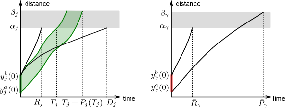
Figure 4: Scheduling parameters in Definition 2. Referring to Figure 1, (αj,βj)subscript𝛼𝑗subscript𝛽𝑗(\alpha_{j},\beta_{j}) is the location of an intersection along the route of vehicle j𝑗j.

By solving Problem 2, the supervisor determines if an override is necessary. If the desired input leads to a set of states at which Problem 2 returns no, the supervisor overrides controlled vehicles with a safe input signal. The two above problems are solved exactly in the next section, and approximately in Section 5.

4 Exact solutions

In this section, we provide the solutions of the verification problem (Problem 2) and the supervisor-design problem (Problem 1). To solve Problem 2, we formulate an Inserted Idle-Time scheduling problem, which is solved straightforwardly, and prove that this problem is equivalent to Problem 2. We then propose a solution to Problem 1.

4.1 Inserted Idle-Time scheduling problem

Problem 2 can be translated into a scheduling problem, considering the intersection as a resource that all vehicles must share. The schedule represents a sequence of the times at which each controlled vehicle enters an intersection, and the idle-times represent the sets of times during which an intersection is potentially occupied by uncontrolled vehicles. This analogy is characterized mathematically using the concept of decision problem equivalence.

Definition 1.

(Cormen et al. (2009)) Consider two decision problems A𝐴A and B𝐵B. The input to a particular problem is called an instance of that problem. Then, A𝐴A is reducible to B𝐵B if there is a procedure that transforms any instance α𝛼\alpha of A𝐴A into some instance β𝛽\beta of B𝐵B in polynomial time, and the answer for α𝛼\alpha is “yes”, denoted by αA𝛼𝐴\alpha\in A, if and only if the answer for β𝛽\beta is “yes”, denoted by βB𝛽𝐵\beta\in B. We say A𝐴A is equivalent to B𝐵B if and only if A𝐴A is reducible to B𝐵B and B𝐵B is reducible to A𝐴A.

An instance I𝐼I of Problem 2 is described by ([𝐱a(0),𝐱b(0)],S)superscript𝐱𝑎0superscript𝐱𝑏0𝑆([\mathbf{x}^{a}(0),\mathbf{x}^{b}(0)],S) where S:=(𝐅,𝐗,𝐘,𝒰,𝒲,𝒟,𝒞,𝒞¯,α1,,αn,β1,,βn)assign𝑆𝐅𝐗𝐘𝒰𝒲𝒟𝒞¯𝒞subscript𝛼1subscript𝛼𝑛subscript𝛽1subscript𝛽𝑛S:=(\mathbf{F,X,Y},\mathcal{U},\mathcal{W},\mathcal{D},\mathcal{C},\bar{\mathcal{C}},\alpha_{1},\ldots,\alpha_{n},\beta_{1},\ldots,\beta_{n}).

To formulate the IIT scheduling problem, we define scheduling parameters.

Definition 2.

Given an initial state estimation [𝐱a(0),𝐱b(0)]superscript𝐱𝑎0superscript𝐱𝑏0[\mathbf{x}^{a}(0),\mathbf{x}^{b}(0)], release times Rjsubscript𝑅𝑗R_{j}, deadlines Djsubscript𝐷𝑗D_{j}, and process times Pj(Tj)subscript𝑃𝑗subscript𝑇𝑗P_{j}(T_{j}) are defined for controlled vehicles. For j𝒞𝑗𝒞j\in\mathcal{C}, if yjb(0)<αjsuperscriptsubscript𝑦𝑗𝑏0subscript𝛼𝑗y_{j}^{b}(0)<\alpha_{j},

Rj:=minuj()𝒰j{t0:yjb(t,uj(),xjb(0))=αj},assignsubscript𝑅𝑗subscriptsubscript𝑢𝑗subscript𝒰𝑗:𝑡0subscriptsuperscript𝑦𝑏𝑗𝑡subscript𝑢𝑗subscriptsuperscript𝑥𝑏𝑗0subscript𝛼𝑗\displaystyle R_{j}:=\min_{{u}_{j}(\cdot)\in\mathcal{U}_{j}}\{t\geq 0:y^{b}_{j}(t,{u}_{j}(\cdot),x^{b}_{j}(0))=\alpha_{j}\},
Dj:=maxuj()𝒰j{t0:yjb(t,uj(),xjb(0))=αj}.assignsubscript𝐷𝑗subscriptsubscript𝑢𝑗subscript𝒰𝑗:𝑡0subscriptsuperscript𝑦𝑏𝑗𝑡subscript𝑢𝑗subscriptsuperscript𝑥𝑏𝑗0subscript𝛼𝑗\displaystyle D_{j}:=\max_{{u}_{j}(\cdot)\in\mathcal{U}_{j}}\{t\geq 0:y^{b}_{j}(t,{u}_{j}(\cdot),x^{b}_{j}(0))=\alpha_{j}\}.

Given a real number Tj>0subscript𝑇𝑗0T_{j}>0,

Pj(Tj):=assignsubscript𝑃𝑗subscript𝑇𝑗absent\displaystyle P_{j}(T_{j}):= minuj()𝒰j{tTj0:\displaystyle\min_{{u}_{j}(\cdot)\in\mathcal{U}_{j}}\{t-T_{j}\geq 0:
yia(t,uj(),xja(0))=βjsubscriptsuperscript𝑦𝑎𝑖𝑡subscript𝑢𝑗subscriptsuperscript𝑥𝑎𝑗0subscript𝛽𝑗\displaystyle y^{a}_{i}(t,{u}_{j}(\cdot),x^{a}_{j}(0))=\beta_{j}
with constraintyjb(Tj,uj(),xjb(0))=αj}.\displaystyle\hskip 21.68121pt\text{with constraint}~{}y^{b}_{j}(T_{j},{u}_{j}(\cdot),x^{b}_{j}(0))=\alpha_{j}\}.

If yjb(0)αjsubscriptsuperscript𝑦𝑏𝑗0subscript𝛼𝑗y^{b}_{j}(0)\geq\alpha_{j}, then Rj=0,Dj=0formulae-sequencesubscript𝑅𝑗0subscript𝐷𝑗0R_{j}=0,D_{j}=0, and Pj(Tj)=minuj()𝒰j{t:yja(t,uj(),xja(0))=βj}subscript𝑃𝑗subscript𝑇𝑗subscriptsubscript𝑢𝑗subscript𝒰𝑗:𝑡subscriptsuperscript𝑦𝑎𝑗𝑡subscript𝑢𝑗subscriptsuperscript𝑥𝑎𝑗0subscript𝛽𝑗P_{j}(T_{j})=\min_{{u}_{j}(\cdot)\in\mathcal{U}_{j}}\{t:y^{a}_{j}(t,{u}_{j}(\cdot),x^{a}_{j}(0))=\beta_{j}\}. If yja(0)βjsubscriptsuperscript𝑦𝑎𝑗0subscript𝛽𝑗y^{a}_{j}(0)\geq\beta_{j}, then set Rj=0,Dj=0formulae-sequencesubscript𝑅𝑗0subscript𝐷𝑗0R_{j}=0,D_{j}=0, and Pj(Tj)=0subscript𝑃𝑗subscript𝑇𝑗0P_{j}(T_{j})=0. If the constraint is not satisfied, set Pj(Tj)=subscript𝑃𝑗subscript𝑇𝑗P_{j}(T_{j})=\infty.

Idle-times (R¯γ,P¯γ)subscript¯𝑅𝛾subscript¯𝑃𝛾(\bar{R}_{\gamma},\bar{P}_{\gamma}) are defined for uncontrolled vehicles. For γ𝒞¯𝛾¯𝒞\gamma\in\bar{\mathcal{C}}, if yγb(0)<αγsubscriptsuperscript𝑦𝑏𝛾0subscript𝛼𝛾y^{b}_{\gamma}(0)<\alpha_{\gamma},

R¯γ:={t0:yγb(t)=αγ},assignsubscript¯𝑅𝛾conditional-set𝑡0subscriptsuperscript𝑦𝑏𝛾𝑡subscript𝛼𝛾\displaystyle\bar{R}_{\gamma}:=\{t\geq 0:y^{b}_{\gamma}(t)=\alpha_{\gamma}\},
P¯γ:={t0:yγa(t)=βγ}.assignsubscript¯𝑃𝛾conditional-set𝑡0subscriptsuperscript𝑦𝑎𝛾𝑡subscript𝛽𝛾\displaystyle\bar{P}_{\gamma}:=\{t\geq 0:y^{a}_{\gamma}(t)=\beta_{\gamma}\}.

If yγb(0)αγsubscriptsuperscript𝑦𝑏𝛾0subscript𝛼𝛾y^{b}_{\gamma}(0)\geq\alpha_{\gamma}, set R¯γ=0subscript¯𝑅𝛾0\bar{R}_{\gamma}=0 and P¯γ={t:yγa(t)=βγ}subscript¯𝑃𝛾conditional-set𝑡subscriptsuperscript𝑦𝑎𝛾𝑡subscript𝛽𝛾\bar{P}_{\gamma}=\{t:y^{a}_{\gamma}(t)=\beta_{\gamma}\}. If yγa(0)βγsubscriptsuperscript𝑦𝑎𝛾0subscript𝛽𝛾y^{a}_{\gamma}(0)\geq\beta_{\gamma}, set R¯γ=0subscript¯𝑅𝛾0\bar{R}_{\gamma}=0 and P¯γ=0subscript¯𝑃𝛾0\bar{P}_{\gamma}=0.

In this definition, release time Rjsubscript𝑅𝑗R_{j} is the earliest that controlled vehicle j𝑗j can enter an intersection while deadline Djsubscript𝐷𝑗D_{j} is the latest. Given that controlled vehicle j𝑗j enters the intersection no earlier than time Tjsubscript𝑇𝑗T_{j}, process time Pj(Tj)subscript𝑃𝑗subscript𝑇𝑗P_{j}(T_{j}) is the earliest that it can cross the intersection. Uncontrolled vehicle γ𝛾\gamma enters and exits the intersection within the idle-time (R¯γ,P¯γ)subscript¯𝑅𝛾subscript¯𝑃𝛾(\bar{R}_{\gamma},\bar{P}_{\gamma}) regardless of its driver-input and disturbance signals. These parameters are illustrated in Figure 4.

The Inserted Idle-time (IIT) scheduling problem is formulated as follows.

Problem 3 ((IIT scheduling)).

Given an initial state estimation [𝐱a(0),𝐱b(0)]superscript𝐱𝑎0superscript𝐱𝑏0[\mathbf{x}^{a}(0),\mathbf{x}^{b}(0)], determine whether there exists a schedule 𝐓=(T1,,Tnc)+nc𝐓subscript𝑇1subscript𝑇subscript𝑛𝑐subscriptsuperscriptsubscript𝑛𝑐\mathbf{T}=(T_{1},\ldots,T_{n_{c}})\in\mathbb{R}^{n_{c}}_{+} such that for all j𝒞𝑗𝒞j\in\mathcal{C},

RjTjDj,subscript𝑅𝑗subscript𝑇𝑗subscript𝐷𝑗R_{j}\leq T_{j}\leq D_{j}, (8)

for all ij𝒞𝑖𝑗𝒞i\neq j\in\mathcal{C},

(Ti,Ti+Pi(Ti))(Tj,Tj+Pj(Tj))=,subscript𝑇𝑖subscript𝑇𝑖subscript𝑃𝑖subscript𝑇𝑖subscript𝑇𝑗subscript𝑇𝑗subscript𝑃𝑗subscript𝑇𝑗(T_{i},T_{i}+P_{i}(T_{i}))\cap(T_{j},T_{j}+P_{j}(T_{j}))=\emptyset, (9)

for all j𝒞𝑗𝒞j\in\mathcal{C} and γ𝒞¯𝛾¯𝒞\gamma\in\bar{\mathcal{C}},

(Tj,Tj+Pj(Tj))(R¯γ,P¯γ)=.subscript𝑇𝑗subscript𝑇𝑗subscript𝑃𝑗subscript𝑇𝑗subscript¯𝑅𝛾subscript¯𝑃𝛾(T_{j},T_{j}+P_{j}(T_{j}))\cap(\bar{R}_{\gamma},\bar{P}_{\gamma})=\emptyset. (10)

Notice that Tjsubscript𝑇𝑗T_{j} and Pj(Tj)subscript𝑃𝑗subscript𝑇𝑗P_{j}(T_{j}) are defined such that for some uj()subscript𝑢𝑗{u}_{j}(\cdot), yjb(Tj,uj(),xjb(0))=αjsuperscriptsubscript𝑦𝑗𝑏subscript𝑇𝑗subscript𝑢𝑗superscriptsubscript𝑥𝑗𝑏0subscript𝛼𝑗y_{j}^{b}(T_{j},{u}_{j}(\cdot),x_{j}^{b}(0))=\alpha_{j} and yja(Tj+Pj(Tj),uj(),xja(0))=βjsuperscriptsubscript𝑦𝑗𝑎subscript𝑇𝑗subscript𝑃𝑗subscript𝑇𝑗subscript𝑢𝑗superscriptsubscript𝑥𝑗𝑎0subscript𝛽𝑗y_{j}^{a}(T_{j}+P_{j}(T_{j}),{u}_{j}(\cdot),x_{j}^{a}(0))=\beta_{j}. Condition (8) represents the constraint induced on the schedule by the bounded input signals. By condition (9), the times during which controlled vehicles i𝑖i and j𝑗j occupy the intersection for any disturbance do not overlap. This implies that a collision between controlled vehicles i𝑖i and j𝑗j is averted. Similarly, condition (10) implies that vehicle j𝑗j does not occupy the intersection during the idle-time, thereby preventing a collision between controlled vehicle j𝑗j and uncontrolled vehicle γ𝛾\gamma. Thus, a schedule satisfying the above conditions is related to an input signal that can prevent any future collision. This is the essence of the proof of the following theorem.

Theorem 1.

Problem 2 and Problem 3 are equivalent.

Proof.

By Definition 1, we need to show two things: Problem 2 is reducible to Problem 3, and Problem 3 is reducible to Problem 2. Notice that an instance I𝐼I of Problem 3 is also described by ([𝐱a(0),𝐱b(0)],S)superscript𝐱𝑎0superscript𝐱𝑏0𝑆([\mathbf{x}^{a}(0),\mathbf{x}^{b}(0)],S), which is the same as an instance of Problem 2. Thus, the transformation between the instances of these problems takes constant time. Now, the following relation is left to prove the equivalence.

IProblem 2I Problem 3.𝐼Problem 2𝐼 Problem 3I\in\text{Problem~{}\ref{problem:verification}}\Leftrightarrow I\in\text{ Problem~{}\ref{problem:scheduling}}.

(\Rightarrow) Given an initial state estimation [𝐱a(0),𝐱b(0)]superscript𝐱𝑎0superscript𝐱𝑏0[\mathbf{x}^{a}(0),\mathbf{x}^{b}(0)], there is an input signal 𝐮~()𝒰~𝐮𝒰\mathbf{\tilde{u}}(\cdot)\in\mathcal{U} such that 𝐲(t,𝐮~(),𝐰(),𝐝(),𝐱(0))B𝐲𝑡~𝐮𝐰𝐝𝐱0𝐵\mathbf{y}(t,\mathbf{\tilde{u}}(\cdot),\mathbf{w}(\cdot),\mathbf{d}(\cdot),\mathbf{x}(0))\notin B for all t𝑡t for any 𝐰()𝒲𝐰𝒲\mathbf{w}(\cdot)\in\mathcal{W} and 𝐝()𝒟𝐝𝒟\mathbf{d}(\cdot)\in\mathcal{D} for any 𝐱(0)[𝐱a(0),𝐱b(0)]𝐱0superscript𝐱𝑎0superscript𝐱𝑏0\mathbf{x}(0)\in[\mathbf{x}^{a}(0),\mathbf{x}^{b}(0)].

Using u~j()subscript~𝑢𝑗{\tilde{u}}_{j}(\cdot) for j𝒞𝑗𝒞j\in\mathcal{C}, which denotes the j𝑗j-th element of 𝐮~()~𝐮\mathbf{\tilde{u}}(\cdot), let T~jsubscript~𝑇𝑗\tilde{T}_{j} be the time at which yjb(t,u~j(),xjb(0))=αjsubscriptsuperscript𝑦𝑏𝑗𝑡subscript~𝑢𝑗subscriptsuperscript𝑥𝑏𝑗0subscript𝛼𝑗y^{b}_{j}(t,{\tilde{u}}_{j}(\cdot),x^{b}_{j}(0))=\alpha_{j} if yjb(0)<αjsubscriptsuperscript𝑦𝑏𝑗0subscript𝛼𝑗y^{b}_{j}(0)<\alpha_{j}. If yjb(0)αjsubscriptsuperscript𝑦𝑏𝑗0subscript𝛼𝑗y^{b}_{j}(0)\geq\alpha_{j}, set T~j=0subscript~𝑇𝑗0\tilde{T}_{j}=0. This satisfies the constraint of Pj(T~j)subscript𝑃𝑗subscript~𝑇𝑗P_{j}(\tilde{T}_{j}) in Definition 2. Let T~j+P~j(T~j)subscript~𝑇𝑗subscript~𝑃𝑗subscript~𝑇𝑗\tilde{T}_{j}+\tilde{P}_{j}(\tilde{T}_{j}) be the time at which yja(t,u~j(),xja(0))=βjsubscriptsuperscript𝑦𝑎𝑗𝑡subscript~𝑢𝑗subscriptsuperscript𝑥𝑎𝑗0subscript𝛽𝑗y^{a}_{j}(t,{\tilde{u}}_{j}(\cdot),x^{a}_{j}(0))=\beta_{j}. Set P~j(T~j)=0subscript~𝑃𝑗subscript~𝑇𝑗0\tilde{P}_{j}(\tilde{T}_{j})=0 if yja(0)βjsubscriptsuperscript𝑦𝑎𝑗0subscript𝛽𝑗y^{a}_{j}(0)\geq\beta_{j}.

By the definitions of Rjsubscript𝑅𝑗R_{j} and Djsubscript𝐷𝑗D_{j}, condition (8) is satisfied. Suppose without loss of generality, T~iT~jsubscript~𝑇𝑖subscript~𝑇𝑗\tilde{T}_{i}\leq\tilde{T}_{j}. At t=T~j𝑡subscript~𝑇𝑗t=\tilde{T}_{j}, we have yjb(t,u~j(),xjb(0))=αjsuperscriptsubscript𝑦𝑗𝑏𝑡subscript~𝑢𝑗subscriptsuperscript𝑥𝑏𝑗0subscript𝛼𝑗y_{j}^{b}(t,{\tilde{u}}_{j}(\cdot),x^{b}_{j}(0))=\alpha_{j}. Since u~i()subscript~𝑢𝑖{\tilde{u}}_{i}(\cdot) and u~j()subscript~𝑢𝑗{\tilde{u}}_{j}(\cdot) guarantee that at most one vehicle is inside an intersection, we must have yia(t,u~i(),xia(0))βisuperscriptsubscript𝑦𝑖𝑎𝑡subscript~𝑢𝑖superscriptsubscript𝑥𝑖𝑎0subscript𝛽𝑖y_{i}^{a}(t,{\tilde{u}}_{i}(\cdot),x_{i}^{a}(0))\geq\beta_{i}. Because yja(t)subscriptsuperscript𝑦𝑎𝑗𝑡y^{a}_{j}(t) is non-decreasing in time, T~i+P~i(T~i)tsubscript~𝑇𝑖subscript~𝑃𝑖subscript~𝑇𝑖𝑡\tilde{T}_{i}+\tilde{P}_{i}(\tilde{T}_{i})\leq t. By the definition of Pi(T~i)subscript𝑃𝑖subscript~𝑇𝑖P_{i}(\tilde{T}_{i}), we have T~i+Pi(T~i)T~i+P~i(T~i)t=T~jsubscript~𝑇𝑖subscript𝑃𝑖subscript~𝑇𝑖subscript~𝑇𝑖subscript~𝑃𝑖subscript~𝑇𝑖𝑡subscript~𝑇𝑗\tilde{T}_{i}+P_{i}(\tilde{T}_{i})\leq\tilde{T}_{i}+\tilde{P}_{i}(\tilde{T}_{i})\leq t=\tilde{T}_{j}, which concludes (T~i,T~i+Pi(T~i))(T~j,T~j+Pj(T~j))=subscript~𝑇𝑖subscript~𝑇𝑖subscript𝑃𝑖subscript~𝑇𝑖subscript~𝑇𝑗subscript~𝑇𝑗subscript𝑃𝑗subscript~𝑇𝑗(\tilde{T}_{i},\tilde{T}_{i}+P_{i}(\tilde{T}_{i}))\cap(\tilde{T}_{j},\tilde{T}_{j}+P_{j}(\tilde{T}_{j}))=\emptyset (condition (9)).

In order to avoid the Bad set, vehicle γ𝒞¯𝛾¯𝒞\gamma\in\bar{\mathcal{C}} is not inside an intersection during [T~j,T~j+P~(T~j)]subscript~𝑇𝑗subscript~𝑇𝑗~𝑃subscript~𝑇𝑗[\tilde{T}_{j},\tilde{T}_{j}+\tilde{P}(\tilde{T}_{j})] for any wγ()𝒲γ,dγ()𝒟γ,formulae-sequencesubscript𝑤𝛾subscript𝒲𝛾subscript𝑑𝛾subscript𝒟𝛾{w}_{\gamma}(\cdot)\in\mathcal{W}_{\gamma},{d}_{\gamma}(\cdot)\in\mathcal{D}_{\gamma}, and xγ(0)[xγa(0),xγb(0)]subscript𝑥𝛾0subscriptsuperscript𝑥𝑎𝛾0subscriptsuperscript𝑥𝑏𝛾0x_{\gamma}(0)\in[x^{a}_{\gamma}(0),x^{b}_{\gamma}(0)]. Since yγb(R¯γ)=αγsuperscriptsubscript𝑦𝛾𝑏subscript¯𝑅𝛾subscript𝛼𝛾y_{\gamma}^{b}(\bar{R}_{\gamma})=\alpha_{\gamma} and yγa(P¯γ)=βγsuperscriptsubscript𝑦𝛾𝑎subscript¯𝑃𝛾subscript𝛽𝛾y_{\gamma}^{a}(\bar{P}_{\gamma})=\beta_{\gamma} by Definition 2, we have (T~j,T~j+P~j(T~j))(R¯γ,P¯γ)=subscript~𝑇𝑗subscript~𝑇𝑗subscript~𝑃𝑗subscript~𝑇𝑗subscript¯𝑅𝛾subscript¯𝑃𝛾(\tilde{T}_{j},\tilde{T}_{j}+\tilde{P}_{j}(\tilde{T}_{j}))\cap(\bar{R}_{\gamma},\bar{P}_{\gamma})=\emptyset. By the definition of Pj(T~j)subscript𝑃𝑗subscript~𝑇𝑗P_{j}(\tilde{T}_{j}), we have (T~j,T~j+Pj(T~j))(T~j,T~j+P~j(T~j))subscript~𝑇𝑗subscript~𝑇𝑗subscript𝑃𝑗subscript~𝑇𝑗subscript~𝑇𝑗subscript~𝑇𝑗subscript~𝑃𝑗subscript~𝑇𝑗(\tilde{T}_{j},\tilde{T}_{j}+P_{j}(\tilde{T}_{j}))\subset(\tilde{T}_{j},\tilde{T}_{j}+\tilde{P}_{j}(\tilde{T}_{j})). Thus, (T~j,T~j+Pj(T~j))(R¯γ,P¯γ)=subscript~𝑇𝑗subscript~𝑇𝑗subscript𝑃𝑗subscript~𝑇𝑗subscript¯𝑅𝛾subscript¯𝑃𝛾(\tilde{T}_{j},\tilde{T}_{j}+P_{j}(\tilde{T}_{j}))\cap(\bar{R}_{\gamma},\bar{P}_{\gamma})=\emptyset. (condition (10)).

This proves that there exists the schedule 𝐓~~𝐓\tilde{\mathbf{T}} that satisfies conditions (8), (9), and (10).

(\Leftarrow) Given an initial state estimation [𝐱a(0),𝐱b(0)]superscript𝐱𝑎0superscript𝐱𝑏0[\mathbf{x}^{a}(0),\mathbf{x}^{b}(0)], there exists a schedule 𝐓~nc~𝐓superscriptsubscript𝑛𝑐\tilde{\mathbf{T}}\in\mathbb{R}^{n_{c}} that satisfies the conditions of Problem 3.

For j𝒞𝑗𝒞j\in\mathcal{C}, define u~j()subscript~𝑢𝑗{\tilde{u}}_{j}(\cdot) such that yjb(T~j,u~j(),xjb(0))=αjsubscriptsuperscript𝑦𝑏𝑗subscript~𝑇𝑗subscript~𝑢𝑗subscriptsuperscript𝑥𝑏𝑗0subscript𝛼𝑗y^{b}_{j}(\tilde{T}_{j},{\tilde{u}}_{j}(\cdot),x^{b}_{j}(0))=\alpha_{j} if yjb(0)<αjsubscriptsuperscript𝑦𝑏𝑗0subscript𝛼𝑗y^{b}_{j}(0)<\alpha_{j}. If yjb(0)αjsubscriptsuperscript𝑦𝑏𝑗0subscript𝛼𝑗y^{b}_{j}(0)\geq\alpha_{j} and yja(0)βjsubscriptsuperscript𝑦𝑎𝑗0subscript𝛽𝑗y^{a}_{j}(0)\leq\beta_{j}, define u~j()subscript~𝑢𝑗{\tilde{u}}_{j}(\cdot) such that yja(T~j+Pj(T~j),u~j(),xja(0))=βjsubscriptsuperscript𝑦𝑎𝑗subscript~𝑇𝑗subscript𝑃𝑗subscript~𝑇𝑗subscript~𝑢𝑗subscriptsuperscript𝑥𝑎𝑗0subscript𝛽𝑗y^{a}_{j}(\tilde{T}_{j}+P_{j}(\tilde{T}_{j}),{\tilde{u}}_{j}(\cdot),x^{a}_{j}(0))=\beta_{j}. If yja(0)>βjsubscriptsuperscript𝑦𝑎𝑗0subscript𝛽𝑗y^{a}_{j}(0)>\beta_{j}, we do not consider vehicle j𝑗j because it has already crossed the intersection. Since yja(t,uj(),xja(0))subscriptsuperscript𝑦𝑎𝑗𝑡subscript𝑢𝑗subscriptsuperscript𝑥𝑎𝑗0y^{a}_{j}(t,{u}_{j}(\cdot),x^{a}_{j}(0)) depends continuously on uj()𝒰jsubscript𝑢𝑗subscript𝒰𝑗{u}_{j}(\cdot)\in\mathcal{U}_{j} and 𝒰jsubscript𝒰𝑗\mathcal{U}_{j} is path connected by Assumption 3, condition (8) implies that such an input signal exists, i.e., u~j()𝒰jsubscript~𝑢𝑗subscript𝒰𝑗{\tilde{u}}_{j}(\cdot)\in\mathcal{U}_{j}.

Consider u~i()subscript~𝑢𝑖{\tilde{u}}_{i}(\cdot) and u~j()subscript~𝑢𝑗{\tilde{u}}_{j}(\cdot) for ij𝒞𝑖𝑗𝒞i\neq j\in\mathcal{C} where T~iT~jsubscript~𝑇𝑖subscript~𝑇𝑗\tilde{T}_{i}\leq\tilde{T}_{j}. Condition (9) says T~i+Pi(T~i)T~jsubscript~𝑇𝑖subscript𝑃𝑖subscript~𝑇𝑖subscript~𝑇𝑗\tilde{T}_{i}+P_{i}(\tilde{T}_{i})\leq\tilde{T}_{j}. At time t[T~i+Pi(T~i),T~j]𝑡subscript~𝑇𝑖subscript𝑃𝑖subscript~𝑇𝑖subscript~𝑇𝑗t\in[\tilde{T}_{i}+P_{i}(\tilde{T}_{i}),\tilde{T}_{j}], we have yia(t,u~i(),xia(0))βisubscriptsuperscript𝑦𝑎𝑖𝑡subscript~𝑢𝑖subscriptsuperscript𝑥𝑎𝑖0subscript𝛽𝑖y^{a}_{i}(t,{\tilde{u}}_{i}(\cdot),x^{a}_{i}(0))\geq\beta_{i} and yjb(t,u~j(),xjb(0))αjsubscriptsuperscript𝑦𝑏𝑗𝑡subscript~𝑢𝑗subscriptsuperscript𝑥𝑏𝑗0subscript𝛼𝑗y^{b}_{j}(t,{\tilde{u}}_{j}(\cdot),x^{b}_{j}(0))\leq\alpha_{j}. Thus, for any disturbance and initial condition, vehicle j𝑗j enters the intersection after vehicle i𝑖i leaves it.

For j𝒞𝑗𝒞j\in\mathcal{C} and γ𝒞¯𝛾¯𝒞\gamma\in\bar{\mathcal{C}}, condition (10) implies either P¯γTjsubscript¯𝑃𝛾subscript𝑇𝑗\bar{P}_{\gamma}\leq T_{j} or T~j+Pj(T~j)R¯γsubscript~𝑇𝑗subscript𝑃𝑗subscript~𝑇𝑗subscript¯𝑅𝛾\tilde{T}_{j}+P_{j}(\tilde{T}_{j})\leq\bar{R}_{\gamma}. In the first case, at any time t[P¯γ,Tj]𝑡subscript¯𝑃𝛾subscript𝑇𝑗t\in[\bar{P}_{\gamma},T_{j}], we have yγa(t)βγsubscriptsuperscript𝑦𝑎𝛾𝑡subscript𝛽𝛾y^{a}_{\gamma}(t)\geq\beta_{\gamma} and yjb(t,u~j(),xjb(0))αjsubscriptsuperscript𝑦𝑏𝑗𝑡subscript~𝑢𝑗subscriptsuperscript𝑥𝑏𝑗0subscript𝛼𝑗y^{b}_{j}(t,{\tilde{u}}_{j}(\cdot),x^{b}_{j}(0))\leq\alpha_{j} so that for any wγ()𝒲γ,dγ()𝒟γ,xγ(0)[xγa(0),xγb(0)]formulae-sequencesubscript𝑤𝛾subscript𝒲𝛾formulae-sequencesubscript𝑑𝛾subscript𝒟𝛾subscript𝑥𝛾0superscriptsubscript𝑥𝛾𝑎0superscriptsubscript𝑥𝛾𝑏0{w}_{\gamma}(\cdot)\in\mathcal{W}_{\gamma},{d}_{\gamma}(\cdot)\in\mathcal{D}_{\gamma},x_{\gamma}(0)\in[x_{\gamma}^{a}(0),x_{\gamma}^{b}(0)] and for any dj()𝒟j,xj(0)[xja(0),xjb(0)]formulae-sequencesubscript𝑑𝑗subscript𝒟𝑗subscript𝑥𝑗0superscriptsubscript𝑥𝑗𝑎0superscriptsubscript𝑥𝑗𝑏0{d}_{j}(\cdot)\in\mathcal{D}_{j},x_{j}(0)\in[x_{j}^{a}(0),x_{j}^{b}(0)], after vehicle γ𝛾\gamma exits the intersection, vehicle j𝑗j enters it. In the second case, at any time t[T~j+Pj(T~j),R¯γ]𝑡subscript~𝑇𝑗subscript𝑃𝑗subscript~𝑇𝑗subscript¯𝑅𝛾t\in[\tilde{T}_{j}+P_{j}(\tilde{T}_{j}),\bar{R}_{\gamma}], we have yja(t,u~j(),xja(0))βjsubscriptsuperscript𝑦𝑎𝑗𝑡subscript~𝑢𝑗subscriptsuperscript𝑥𝑎𝑗0subscript𝛽𝑗y^{a}_{j}(t,{\tilde{u}}_{j}(\cdot),x^{a}_{j}(0))\geq\beta_{j} and yγb(t)αγsubscriptsuperscript𝑦𝑏𝛾𝑡subscript𝛼𝛾y^{b}_{\gamma}(t)\leq\alpha_{\gamma}. This means after vehicle j𝑗j exits the intersection for any dj()𝒟jsubscript𝑑𝑗subscript𝒟𝑗{d}_{j}(\cdot)\in\mathcal{D}_{j} and xj(0)[xja(0),xjb(0)]subscript𝑥𝑗0superscriptsubscript𝑥𝑗𝑎0superscriptsubscript𝑥𝑗𝑏0x_{j}(0)\in[x_{j}^{a}(0),x_{j}^{b}(0)], vehicle γ𝛾\gamma enters it for any wγ()𝒲γ,dγ()𝒟γ,formulae-sequencesubscript𝑤𝛾subscript𝒲𝛾subscript𝑑𝛾subscript𝒟𝛾{w}_{\gamma}(\cdot)\in\mathcal{W}_{\gamma},{d}_{\gamma}(\cdot)\in\mathcal{D}_{\gamma}, and xγ(0)[xγa(0),xγb(0)]subscript𝑥𝛾0superscriptsubscript𝑥𝛾𝑎0superscriptsubscript𝑥𝛾𝑏0x_{\gamma}(0)\in[x_{\gamma}^{a}(0),x_{\gamma}^{b}(0)].

Therefore, the schedule 𝐓~~𝐓\tilde{\mathbf{T}} ensures that there exists an input signal 𝐮~()~𝐮\mathbf{\tilde{u}}(\cdot) which prevents entering the Bad set. ∎∎

We now provide an algorithm that solves Problem 3, which, in turn, solves Problem 2 by Theorem 1. This algorithm contains two procedures. The first procedure, Scheduling, generates a schedule 𝐓𝐓\mathbf{T} given a sequence π𝜋\pi such that TπiTπjsubscript𝑇subscript𝜋𝑖subscript𝑇subscript𝜋𝑗T_{\pi_{i}}\leq T_{\pi_{j}} if i<j𝑖𝑗i<j, and evaluates whether 𝐓𝐓\mathbf{T} satisfies conditions (8)-(10). Here, πisubscript𝜋𝑖\pi_{i} denotes the i𝑖i-th entry of π𝜋\pi and Tπisubscript𝑇subscript𝜋𝑖T_{\pi_{i}} the πisubscript𝜋𝑖\pi_{i}-entry of 𝐓𝐓\mathbf{T}. The second procedure, Exact, inspects all possible sequences until a sequence with a feasible schedule is found. If a feasible schedule is found, the answer of Problem 2 is yes, and otherwise, the answer is no.

Algorithm 1 focuses on vehicles before an intersection. The set of such vehicles is denoted by :={j𝒞:yjb(0)<αj}assignconditional-set𝑗𝒞superscriptsubscript𝑦𝑗𝑏0subscript𝛼𝑗\mathcal{M}:=\{j\in\mathcal{C}:y_{j}^{b}(0)<\alpha_{j}\}. For simplicity, let yjb(0)<αjsubscriptsuperscript𝑦𝑏𝑗0subscript𝛼𝑗y^{b}_{j}(0)<\alpha_{j} for j{1,,||}𝑗1j\in\{1,\ldots,|\mathcal{M}|\} and yjb(0)αjsubscriptsuperscript𝑦𝑏𝑗0subscript𝛼𝑗y^{b}_{j}(0)\geq\alpha_{j} for j{||+1,,nc}𝑗1subscript𝑛𝑐j\in\{|\mathcal{M}|+1,\ldots,n_{c}\}. Let 𝒫𝒫\mathcal{P} be a set of all permutations of \mathcal{M}. Its cardinality is (||)!=1×2××||12(|\mathcal{M}|)!=1\times 2\times\ldots\times|\mathcal{M}|. Let π||𝜋superscript\pi\in\mathbb{R}^{|\mathcal{M}|} be a vector in 𝒫𝒫\mathcal{P}. Let π¯nc¯¯𝜋superscriptsubscript𝑛¯𝑐\bar{\pi}\in\mathbb{R}^{n_{\bar{c}}} be a vector of γ𝒞¯𝛾¯𝒞\gamma\in\bar{\mathcal{C}} in an increasing order of R¯γsubscript¯𝑅𝛾\bar{R}_{\gamma}, that is, R¯π¯jR¯π¯jsubscript¯𝑅subscript¯𝜋𝑗subscript¯𝑅subscript¯𝜋superscript𝑗\bar{R}_{\bar{\pi}_{j}}\leq\bar{R}_{\bar{\pi}_{j^{\prime}}} for jj𝑗superscript𝑗j\leq j^{\prime}. Let π0,jsubscript𝜋0𝑗\pi_{0,j} and π¯jsubscript¯𝜋𝑗\bar{\pi}_{j} denote the j𝑗j-th entry of π0subscript𝜋0\pi_{0} and π¯¯𝜋\bar{\pi}, respectively.

Refer to caption
Figure 5: Schematic of the supervisor at time kτ𝑘𝜏k\tau. Using the state measurement 𝐱m(kτ)subscript𝐱𝑚𝑘𝜏\mathbf{x}_{m}(k\tau) and the previous step’s state prediction 𝐗pred(𝐮outk1())subscript𝐗𝑝𝑟𝑒𝑑subscriptsuperscript𝐮𝑘1𝑜𝑢𝑡\mathbf{X}_{pred}(\mathbf{u}^{{k-1}}_{out}(\cdot)), the state estimation is corrected to [𝐱a(kτ),𝐱b(kτ)]superscript𝐱𝑎𝑘𝜏superscript𝐱𝑏𝑘𝜏[\mathbf{x}^{a}(k\tau),\mathbf{x}^{b}(k\tau)]. The supervisor takes [𝐱a(kτ),𝐱b(kτ)]superscript𝐱𝑎𝑘𝜏superscript𝐱𝑏𝑘𝜏[\mathbf{x}^{a}(k\tau),\mathbf{x}^{b}(k\tau)] and the current desired input 𝐮desireksuperscriptsubscript𝐮𝑑𝑒𝑠𝑖𝑟𝑒𝑘\mathbf{u}_{desire}^{k} and returns either 𝐮desirek()superscriptsubscript𝐮𝑑𝑒𝑠𝑖𝑟𝑒𝑘\mathbf{u}_{desire}^{k}(\cdot) or 𝐮safek()subscriptsuperscript𝐮𝑘𝑠𝑎𝑓𝑒\mathbf{u}^{{k}}_{safe}(\cdot) depending on the answer of the verification problem. When the answer is no, the state prediction 𝐗pred(𝐮safek())subscript𝐗𝑝𝑟𝑒𝑑subscriptsuperscript𝐮𝑘𝑠𝑎𝑓𝑒\mathbf{X}_{pred}(\mathbf{u}^{{k}}_{safe}(\cdot)) guarantees the existence of a feasible schedule 𝐓2subscript𝐓2\mathbf{T}_{2}, thereby ensuring the non-blocking property of the supervisor. At each step, a safe input signal 𝐮safek+1()subscriptsuperscript𝐮𝑘1𝑠𝑎𝑓𝑒\mathbf{u}^{{k+1}}_{safe}(\cdot) is generated using a feasible schedule and stored for a possible use at the next step.
1:procedure Scheduling(π0,[𝐱a(0),𝐱b(0)],Ssubscript𝜋0superscript𝐱𝑎0superscript𝐱𝑏0𝑆\pi_{0},[\mathbf{x}^{a}(0),\mathbf{x}^{b}(0)],S)
2:    for all j𝒞𝑗𝒞j\in\mathcal{C} do calculate Rj,Djsubscript𝑅𝑗subscript𝐷𝑗R_{j},D_{j}     
3:    for all γ𝒞¯𝛾¯𝒞\gamma\in\bar{\mathcal{C}} do calculate R¯γ,P¯γsubscript¯𝑅𝛾subscript¯𝑃𝛾\bar{R}_{\gamma},\bar{P}_{\gamma}     
4:    ={j𝒞:yjb(0)<αj}conditional-set𝑗𝒞subscriptsuperscript𝑦𝑏𝑗0subscript𝛼𝑗\mathcal{M}=\{j\in\mathcal{C}:y^{b}_{j}(0)<\alpha_{j}\} and ¯=𝒞¯𝒞\bar{\mathcal{M}}=\mathcal{C}\setminus\mathcal{M}
5:    Tj=0j¯subscript𝑇𝑗0for-all𝑗¯T_{j}=0~{}\forall~{}j\in\bar{\mathcal{M}} and Pmax=maxj¯Pj(Tj)subscript𝑃𝑚𝑎𝑥subscript𝑗¯subscript𝑃𝑗subscript𝑇𝑗P_{max}=\max_{j\in\bar{\mathcal{M}}}P_{j}(T_{j})
6:    π=(π0,j:π0,jforj=1to|π0|)\pi=(\pi_{0,j}:\pi_{0,j}\in\mathcal{M}~{}\text{for}~{}j=1~{}\text{to}~{}|\pi_{0}|)
7:    for i=1𝑖1i=1 to |||\mathcal{M}| do
8:       if i=1𝑖1i=1 then Tπ1=max(Rπ1,Pmax)subscript𝑇subscript𝜋1subscript𝑅subscript𝜋1subscript𝑃𝑚𝑎𝑥T_{\pi_{1}}=\max(R_{\pi_{1}},P_{max})
9:       else if i2𝑖2i\geq 2 then
10:           Tπi=max(Rπi,Tπi1+Pπi1(Tπi1))subscript𝑇subscript𝜋𝑖subscript𝑅subscript𝜋𝑖subscript𝑇subscript𝜋𝑖1subscript𝑃subscript𝜋𝑖1subscript𝑇subscript𝜋𝑖1T_{\pi_{i}}=\max(R_{\pi_{i}},T_{\pi_{i-1}}+P_{\pi_{i-1}}(T_{\pi_{i-1}}))        
11:       for j=1𝑗1j=1 to nc¯subscript𝑛¯𝑐n_{\bar{c}} do
12:           if TπiR¯π¯jsubscript𝑇subscript𝜋𝑖subscript¯𝑅subscript¯𝜋𝑗T_{\pi_{i}}\geq\bar{R}_{\bar{\pi}_{j}} then
13:              Tπi=max(Tπi,P¯π¯j)subscript𝑇subscript𝜋𝑖subscript𝑇subscript𝜋𝑖subscript¯𝑃subscript¯𝜋𝑗T_{\pi_{i}}=\max(T_{\pi_{i}},\bar{P}_{\bar{\pi}_{j}})
14:           else if Tπi+Pπi(Tπi)>R¯π¯jsubscript𝑇subscript𝜋𝑖subscript𝑃subscript𝜋𝑖subscript𝑇subscript𝜋𝑖subscript¯𝑅subscript¯𝜋𝑗T_{\pi_{i}}+P_{\pi_{i}}(T_{\pi_{i}})>\bar{R}_{\bar{\pi}_{j}} then
15:              Tπi=P¯π¯jsubscript𝑇subscript𝜋𝑖subscript¯𝑃subscript¯𝜋𝑗T_{\pi_{i}}=\bar{P}_{\bar{\pi}_{j}}                        
16:    if TjDjsubscript𝑇𝑗subscript𝐷𝑗T_{j}\leq D_{j} for all j𝒞𝑗𝒞j\in\mathcal{C} then return (𝐓,yes)𝐓𝑦𝑒𝑠(\mathbf{T},yes)     
17:    return (,no)𝑛𝑜(\emptyset,no)
18:procedure Exact([𝐱a(0),𝐱b(0)],Ssuperscript𝐱𝑎0superscript𝐱𝑏0𝑆[\mathbf{x}^{a}(0),\mathbf{x}^{b}(0)],S)
19:    if [𝐲a(0),𝐲b(0)]Bsuperscript𝐲𝑎0superscript𝐲𝑏0𝐵[\mathbf{y}^{a}(0),\mathbf{y}^{b}(0)]\cap B\neq\emptyset then return (,no)𝑛𝑜(\emptyset,no)     
20:    ={j𝒞:yjb(0)<αj}conditional-set𝑗𝒞subscriptsuperscript𝑦𝑏𝑗0subscript𝛼𝑗\mathcal{M}=\{j\in\mathcal{C}:y^{b}_{j}(0)<\alpha_{j}\} and ¯=𝒞¯𝒞\bar{\mathcal{M}}=\mathcal{C}\setminus\mathcal{M}
21:    if ||=00|\mathcal{M}|=0 then return (,yes)𝑦𝑒𝑠(\emptyset,yes)     
22:    for all π𝒫𝜋𝒫\pi\in\mathcal{P} do
23:       (𝐓,ans)=Scheduling(π,[𝐱a(0),𝐱b(0)],S)𝐓𝑎𝑛𝑠Scheduling𝜋superscript𝐱𝑎0superscript𝐱𝑏0𝑆(\mathbf{T},ans)=\textsc{Scheduling}(\pi,[\mathbf{x}^{a}(0),\mathbf{x}^{b}(0)],S)
24:       if ans=yes𝑎𝑛𝑠𝑦𝑒𝑠ans=yes then return (𝐓,yes)𝐓𝑦𝑒𝑠(\mathbf{T},yes)            
25:    return (,no)𝑛𝑜(\emptyset,no)
Algorithm 1 Exact Solution of Problem 3

Procedure Scheduling in Algorithm 1 works as follows. In lines 2-3, the scheduling parameters in Definition 2 are computed given an initial state estimation. In lines 4 and 5, if yjb(0)αjsubscriptsuperscript𝑦𝑏𝑗0subscript𝛼𝑗y^{b}_{j}(0)\geq\alpha_{j}, Tj=0subscript𝑇𝑗0T_{j}=0 because Rj=Dj=0subscript𝑅𝑗subscript𝐷𝑗0R_{j}=D_{j}=0 and Pmaxsubscript𝑃𝑚𝑎𝑥P_{max} is the time at which all vehicles j¯𝑗¯j\in\bar{\mathcal{M}} exit the intersection. The input argument π0subscript𝜋0\pi_{0} is the vector of the indexes of all vehicles controlled by the supervisor. The assignment at line 6 extracts from π0subscript𝜋0\pi_{0} the sub-vector π𝜋\pi of vehicles which have not yet reached the intersection. The schedule needs only be computed for the sub-vector π𝜋\pi.

In a given sequence π𝜋\pi, vehicle πi1subscript𝜋𝑖1\pi_{i-1} crosses the intersection earlier than vehicle πisubscript𝜋𝑖\pi_{i}. Given this sequence π𝜋\pi, procedure Scheduling finds the earliest possible schedule. In the for loop of lines 11-15, uncontrolled vehicle π¯jsubscript¯𝜋𝑗\bar{\pi}_{j} is considered. If line 12 is true, then line 13 ensures that TπiP¯π¯jsubscript𝑇subscript𝜋𝑖subscript¯𝑃subscript¯𝜋𝑗T_{\pi_{i}}\geq\bar{P}_{\bar{\pi}_{j}} so that condition (10) is satisfied. Otherwise, if line 14 is true, meaning that Tπi<R¯π¯j<Tπi+Pπi(Tπi)subscript𝑇subscript𝜋𝑖subscript¯𝑅subscript¯𝜋𝑗subscript𝑇subscript𝜋𝑖subscript𝑃subscript𝜋𝑖subscript𝑇subscript𝜋𝑖T_{\pi_{i}}<\bar{R}_{\bar{\pi}_{j}}<T_{\pi_{i}}+P_{\pi_{i}}(T_{\pi_{i}}), then Tπisubscript𝑇subscript𝜋𝑖T_{\pi_{i}} is delayed to P¯π¯jsubscript¯𝑃subscript¯𝜋𝑗\bar{P}_{\bar{\pi}_{j}} in line 15 so that condition (10) becomes satisfied. The schedule Tπisubscript𝑇subscript𝜋𝑖T_{\pi_{i}} takes P¯π¯jsubscript¯𝑃subscript¯𝜋𝑗\bar{P}_{\bar{\pi}_{j}}, which is the earliest possible value. Otherwise, Tπi+Pπi(Tπi)R¯π¯jsubscript𝑇subscript𝜋𝑖subscript𝑃subscript𝜋𝑖subscript𝑇subscript𝜋𝑖subscript¯𝑅subscript¯𝜋𝑗T_{\pi_{i}}+P_{\pi_{i}}(T_{\pi_{i}})\leq\bar{R}_{\bar{\pi}_{j}} so that condition (10) is guaranteed. Lastly, in line 16, the right inequality of condition (8) is checked. If line 16 is true, this procedure returns a feasible schedule and answer yes. If Tj>Djsubscript𝑇𝑗subscript𝐷𝑗T_{j}>D_{j} for some j𝑗j, since the schedule 𝐓𝐓\mathbf{T} is constructed so that it is the earliest possible value, there cannot be another schedule 𝐓~~𝐓\tilde{\mathbf{T}} such that T~jDjsubscript~𝑇𝑗subscript𝐷𝑗\tilde{T}_{j}\leq D_{j}. Thus, no feasible schedule can be found in this sequence π𝜋\pi, and the procedure returns no.

Procedure Exact in Algorithm 1 solves Problem 3 by inspecting all permutations in 𝒫𝒫\mathcal{P} until a feasible schedule is found as noted in lines 22-24. In line 19, if a given initial position estimation is already inside the Bad set, the procedure returns no. In line 21, if yjb(0)αjsubscriptsuperscript𝑦𝑏𝑗0subscript𝛼𝑗y^{b}_{j}(0)\geq\alpha_{j} for all j𝒞𝑗𝒞j\in\mathcal{C}, then it returns yes since all controlled vehicles have entered the intersection. If no feasible schedule is found after evaluating all permutations in 𝒫𝒫\mathcal{P}, an empty set and answer no are returned in line 25.

The running time of procedure Exact is determined by the for loops of lines 22-24. For the worst case, all permutations in 𝒫𝒫\mathcal{P} must be evaluated. As the number of controlled vehicles increases, the computation time increases exponentially. Indeed, a scheduling problem is known to be NP-hard (Colombo and Del Vecchio (2012)). To avoid this computational complexity issue, we devise an approximate algorithm to solve the IIT scheduling problem with the guarantee of a quantified approximation bound. This approximate algorithm is provided in Section 5.1.

4.2 Exact supervisor

In this section, we solve Problem 1 by providing an algorithm implementing the exact supervisor.

The schematic of a supervisor at time kτ𝑘𝜏k\tau is illustrated in Figure 5. The state prediction computed at the previous step 𝐗pred(𝐮outk1())subscript𝐗𝑝𝑟𝑒𝑑subscriptsuperscript𝐮𝑘1𝑜𝑢𝑡\mathbf{X}_{pred}(\mathbf{u}^{{k-1}}_{out}(\cdot)) is known, where 𝐮outk1()subscriptsuperscript𝐮𝑘1𝑜𝑢𝑡\mathbf{u}^{{k-1}}_{out}(\cdot) is the output that the supervisor returns at the previous step, that is, controlled vehicles traveled with 𝐮outk1()subscriptsuperscript𝐮𝑘1𝑜𝑢𝑡\mathbf{u}^{{k-1}}_{out}(\cdot) for time [(k1)τ,kτ)𝑘1𝜏𝑘𝜏[(k-1)\tau,k\tau). Also, the state measurement 𝐱m(kτ)subscript𝐱𝑚𝑘𝜏\mathbf{x}_{m}(k\tau) is received. These state prediction and measurement are used to update the state estimation [𝐱a(kτ),𝐱b(kτ)]superscript𝐱𝑎𝑘𝜏superscript𝐱𝑏𝑘𝜏[\mathbf{x}^{a}(k\tau),\mathbf{x}^{b}(k\tau)]. This state estimation and the desired input 𝐮desireksuperscriptsubscript𝐮𝑑𝑒𝑠𝑖𝑟𝑒𝑘\mathbf{u}_{desire}^{k} are the inputs to the supervisor and used to predict the state at the next time step, denoted by 𝐗pred(𝐮desirek())subscript𝐗𝑝𝑟𝑒𝑑superscriptsubscript𝐮𝑑𝑒𝑠𝑖𝑟𝑒𝑘\mathbf{X}_{pred}(\mathbf{u}_{desire}^{k}(\cdot)). Given this state prediction, the verification problem is solved. If the answer is yes, the supervisor allows the controlled vehicles to travel with the desired input for time [kτ,(k+1)τ)𝑘𝜏𝑘1𝜏[k\tau,(k+1)\tau). A safe input signal 𝐮safek+1()subscriptsuperscript𝐮𝑘1𝑠𝑎𝑓𝑒\mathbf{u}^{{k+1}}_{safe}(\cdot) is generated using a feasible schedule 𝐓1subscript𝐓1\mathbf{T}_{1} and stored for a possible use at the next time step. If the answer is no, a safe input signal 𝐮safek()subscriptsuperscript𝐮𝑘𝑠𝑎𝑓𝑒\mathbf{u}^{{k}}_{safe}(\cdot) stored at the previous step is used to override the controlled vehicles. It will be proved in this section that the state prediction 𝐗pred(𝐮safek())subscript𝐗𝑝𝑟𝑒𝑑subscriptsuperscript𝐮𝑘𝑠𝑎𝑓𝑒\mathbf{X}_{pred}(\mathbf{u}^{{k}}_{safe}(\cdot)) always has a feasible schedule 𝐓2subscript𝐓2\mathbf{T}_{2}, that is, 𝐗pred(𝐮safek())subscript𝐗𝑝𝑟𝑒𝑑subscriptsuperscript𝐮𝑘𝑠𝑎𝑓𝑒absent\mathbf{X}_{pred}(\mathbf{u}^{{k}}_{safe}(\cdot))\in Problem 2. A safe input signal 𝐮safek+1()subscriptsuperscript𝐮𝑘1𝑠𝑎𝑓𝑒\mathbf{u}^{{k+1}}_{safe}(\cdot) is generated using 𝐓2subscript𝐓2\mathbf{T}_{2} and stored. The output 𝐮outk()subscriptsuperscript𝐮𝑘𝑜𝑢𝑡\mathbf{u}^{{k}}_{out}(\cdot) is either 𝐮desirek()superscriptsubscript𝐮𝑑𝑒𝑠𝑖𝑟𝑒𝑘\mathbf{u}_{desire}^{k}(\cdot) or 𝐮safek()subscriptsuperscript𝐮𝑘𝑠𝑎𝑓𝑒\mathbf{u}^{{k}}_{safe}(\cdot), and the state prediction 𝐗pred(𝐮outk())subscript𝐗𝑝𝑟𝑒𝑑subscriptsuperscript𝐮𝑘𝑜𝑢𝑡\mathbf{X}_{pred}(\mathbf{u}^{{k}}_{out}(\cdot)) will be used at the next step to correct the state estimation with a new state measurement.

In the last section, we presented Algorithm 1 that solves the verification problem. This section describes the remaining components: state prediction, correction of the state estimation, and a safe input generator. Also, an algorithm to implement the supervisor is presented with the proof that this supervisor is the solution of Problem 1.

4.2.1 State prediction.

Using the dynamic model (1), this function predicts the state reached at the next time step with a given input signal starting from a set of states. Suppose that at time kτ𝑘𝜏k\tau, we have the state estimation [𝐱a(kτ),𝐱b(kτ)]superscript𝐱𝑎𝑘𝜏superscript𝐱𝑏𝑘𝜏[\mathbf{x}^{a}(k\tau),\mathbf{x}^{b}(k\tau)] and the input 𝐮k()𝒰superscript𝐮𝑘𝒰\mathbf{u}^{k}(\cdot)\in\mathcal{U} defined on time [kτ,(k+1)τ)𝑘𝜏𝑘1𝜏[k\tau,(k+1)\tau). The state prediction 𝐗pred(𝐮k())=[min𝐗pred(𝐮k()),max𝐗pred(𝐮k())]𝐗subscript𝐗𝑝𝑟𝑒𝑑superscript𝐮𝑘subscript𝐗𝑝𝑟𝑒𝑑superscript𝐮𝑘subscript𝐗𝑝𝑟𝑒𝑑superscript𝐮𝑘𝐗\mathbf{X}_{pred}(\mathbf{u}^{k}(\cdot))=[\min\mathbf{X}_{pred}(\mathbf{u}^{k}(\cdot)),\max\mathbf{X}_{pred}(\mathbf{u}^{k}(\cdot))]\subset\mathbf{X} is a set of possible states at the next time step. Its i𝑖i-th set is denoted by Xpred,i(uik())=[minXpred,i(uik()),maxXpred,i(uik())]subscript𝑋𝑝𝑟𝑒𝑑𝑖subscriptsuperscript𝑢𝑘𝑖subscript𝑋𝑝𝑟𝑒𝑑𝑖subscriptsuperscript𝑢𝑘𝑖subscript𝑋𝑝𝑟𝑒𝑑𝑖subscriptsuperscript𝑢𝑘𝑖X_{pred,i}(u^{k}_{i}(\cdot))=[\min X_{pred,i}(u^{k}_{i}(\cdot)),\max X_{pred,i}(u^{k}_{i}(\cdot))]. The state prediction is defined as follows: for j𝒞𝑗𝒞j\in\mathcal{C},

minXpred,j(ujk())=mindj()𝒟jxj(τ,ujk(),dj(),xja(kτ)),maxXpred,j(ujk())=maxdj()𝒟jxj(τ,ujk(),dj(),xjb(kτ)).formulae-sequencesubscript𝑋𝑝𝑟𝑒𝑑𝑗subscriptsuperscript𝑢𝑘𝑗subscriptsubscript𝑑𝑗subscript𝒟𝑗subscript𝑥𝑗𝜏superscriptsubscript𝑢𝑗𝑘subscript𝑑𝑗subscriptsuperscript𝑥𝑎𝑗𝑘𝜏subscript𝑋𝑝𝑟𝑒𝑑𝑗subscriptsuperscript𝑢𝑘𝑗subscriptsubscript𝑑𝑗subscript𝒟𝑗subscript𝑥𝑗𝜏superscriptsubscript𝑢𝑗𝑘subscript𝑑𝑗subscriptsuperscript𝑥𝑏𝑗𝑘𝜏\displaystyle\begin{split}&\min{X_{pred,j}(u^{k}_{j}(\cdot))}=\min_{{d}_{j}(\cdot)\in\mathcal{D}_{j}}x_{j}(\tau,u_{j}^{k}(\cdot),{d}_{j}(\cdot),x^{a}_{j}(k\tau)),\\ &\max{X_{pred,j}(u^{k}_{j}(\cdot))}=\max_{{d}_{j}(\cdot)\in\mathcal{D}_{j}}x_{j}(\tau,u_{j}^{k}(\cdot),{d}_{j}(\cdot),x^{b}_{j}(k\tau)).\end{split} (11)

For γ𝒞¯,𝛾¯𝒞\gamma\in\bar{\mathcal{C}},

minXpred,γ=minwγ()𝒲γ,dγ()𝒟γxγ(τ,wγ(),dγ(),xγa(kτ)),maxXpred,γ=maxwγ()𝒲γ,dγ()𝒟γxγ(τ,wγ(),dγ(),xγb(kτ)).formulae-sequencesubscript𝑋𝑝𝑟𝑒𝑑𝛾subscriptsubscript𝑤𝛾subscript𝒲𝛾subscript𝑑𝛾subscript𝒟𝛾subscript𝑥𝛾𝜏subscript𝑤𝛾subscript𝑑𝛾subscriptsuperscript𝑥𝑎𝛾𝑘𝜏subscript𝑋𝑝𝑟𝑒𝑑𝛾subscriptsubscript𝑤𝛾subscript𝒲𝛾subscript𝑑𝛾subscript𝒟𝛾subscript𝑥𝛾𝜏subscript𝑤𝛾subscript𝑑𝛾subscriptsuperscript𝑥𝑏𝛾𝑘𝜏\displaystyle\begin{split}&\min{X_{pred,\gamma}}=\min_{\begin{subarray}{a}{w}_{\gamma}(\cdot)\in\mathcal{W}_{\gamma},\\ {d}_{\gamma}(\cdot)\in\mathcal{D}_{\gamma}\end{subarray}}x_{\gamma}(\tau,{w}_{\gamma}(\cdot),{d}_{\gamma}(\cdot),x^{a}_{\gamma}(k\tau)),\\ &\max{X_{pred,\gamma}}=\max_{\begin{subarray}{a}{w}_{\gamma}(\cdot)\in\mathcal{W}_{\gamma},\\ {d}_{\gamma}(\cdot)\in\mathcal{D}_{\gamma}\end{subarray}}x_{\gamma}(\tau,{w}_{\gamma}(\cdot),{d}_{\gamma}(\cdot),x^{b}_{\gamma}(k\tau)).\end{split} (12)

By definition, min𝐗pred(𝐮k())subscript𝐗𝑝𝑟𝑒𝑑superscript𝐮𝑘\min\mathbf{X}_{pred}(\mathbf{u}^{k}(\cdot)) is the smallest state propagated from 𝐱a(kτ)superscript𝐱𝑎𝑘𝜏\mathbf{x}^{a}(k\tau) for time τ𝜏\tau with the input 𝐮k()superscript𝐮𝑘\mathbf{u}^{k}(\cdot) for any disturbance and any driver-input of uncontrolled vehicles, and max𝐗pred(𝐮k())subscript𝐗𝑝𝑟𝑒𝑑superscript𝐮𝑘\max\mathbf{X}_{pred}(\mathbf{u}^{k}(\cdot)) is the largest.

Notice that Exact(𝐗pred(𝐮desirek()),S)subscript𝐗𝑝𝑟𝑒𝑑superscriptsubscript𝐮𝑑𝑒𝑠𝑖𝑟𝑒𝑘𝑆(\mathbf{X}_{pred}(\mathbf{u}_{desire}^{k}(\cdot)),S) in Algorithm 1 determines the existence of an input signal 𝐮safek+1,()subscriptsuperscript𝐮𝑘1𝑠𝑎𝑓𝑒\mathbf{u}^{{k+1,\infty}}_{safe}(\cdot) that satisfies 𝐲(t,𝐮safek+1,(),𝐰(),𝐝(),𝐱((k+1)τ))B𝐲𝑡subscriptsuperscript𝐮𝑘1𝑠𝑎𝑓𝑒𝐰𝐝𝐱𝑘1𝜏𝐵\mathbf{y}(t,\mathbf{u}^{{k+1,\infty}}_{safe}(\cdot),\mathbf{w}(\cdot),\mathbf{d}(\cdot),\mathbf{x}((k+1)\tau))\notin B for all t𝑡t for any 𝐰()𝐰\mathbf{w}(\cdot) and 𝐝()𝐝\mathbf{d}(\cdot) for any 𝐱((k+1)τ)𝐗pred(𝐮desirek)𝐱𝑘1𝜏subscript𝐗𝑝𝑟𝑒𝑑superscriptsubscript𝐮𝑑𝑒𝑠𝑖𝑟𝑒𝑘\mathbf{x}((k+1)\tau)\in\mathbf{X}_{pred}(\mathbf{u}_{desire}^{k}). If we define 𝐮desirek,()subscriptsuperscript𝐮𝑘𝑑𝑒𝑠𝑖𝑟𝑒\mathbf{u}^{{k},\infty}_{desire}(\cdot) as

𝐮desirek,(t)={𝐮desirekfort[kτ,(k+1)τ),𝐮safek+1,(t)fort[(k+1)τ,),superscriptsubscript𝐮𝑑𝑒𝑠𝑖𝑟𝑒𝑘𝑡casessuperscriptsubscript𝐮𝑑𝑒𝑠𝑖𝑟𝑒𝑘for𝑡𝑘𝜏𝑘1𝜏superscriptsubscript𝐮𝑠𝑎𝑓𝑒𝑘1𝑡for𝑡𝑘1𝜏\mathbf{u}_{desire}^{k,\infty}(t)=\begin{cases}\mathbf{u}_{desire}^{k}&\text{for}~{}t\in[k\tau,(k+1)\tau),\\ \mathbf{u}_{safe}^{k+1,\infty}(t)&\text{for}~{}t\in[(k+1)\tau,\infty),\end{cases} (13)

then 𝐲(t,𝐮desirek,(),𝐰(),𝐝(),𝐱(kτ))B𝐲𝑡subscriptsuperscript𝐮𝑘𝑑𝑒𝑠𝑖𝑟𝑒𝐰𝐝𝐱𝑘𝜏𝐵\mathbf{y}(t,\mathbf{u}^{{k},\infty}_{desire}(\cdot),\mathbf{w}(\cdot),\mathbf{d}(\cdot),\mathbf{x}(k\tau))\notin B for all t𝑡t for any 𝐰()𝐰\mathbf{w}(\cdot) and 𝐝()𝐝\mathbf{d}(\cdot) for any 𝐱(kτ)[𝐱a(kτ),𝐱b(kτ)]𝐱𝑘𝜏superscript𝐱𝑎𝑘𝜏superscript𝐱𝑏𝑘𝜏\mathbf{x}(k\tau)\in[\mathbf{x}^{a}(k\tau),\mathbf{x}^{b}(k\tau)].

4.2.2 Correction of the state estimation.

Once a new state measurement is received, this function restricts the state estimation so that it is compatible with the state measurement and the state prediction computed at the previous step. Suppose the supervisor returns 𝐮outk1()subscriptsuperscript𝐮𝑘1𝑜𝑢𝑡\mathbf{u}^{{k-1}}_{out}(\cdot) at time (k1)τ𝑘1𝜏(k-1)\tau. Then, at time kτ𝑘𝜏k\tau, we have 𝐱(kτ)𝐗pred(𝐮outk1())𝐱𝑘𝜏subscript𝐗𝑝𝑟𝑒𝑑subscriptsuperscript𝐮𝑘1𝑜𝑢𝑡\mathbf{x}(k\tau)\in\mathbf{X}_{pred}(\mathbf{u}^{{k-1}}_{out}(\cdot)) by definitions (LABEL:equation:stateprediction_j) and (LABEL:equation:stateprediction_gamma). Also, a new state measurement 𝐱m(kτ)subscript𝐱𝑚𝑘𝜏\mathbf{x}_{m}(k\tau) is received, which implies 𝐱(kτ)[𝐱m(kτ)+δmin,𝐱m(kτ)+δmax]𝐱𝑘𝜏subscript𝐱𝑚𝑘𝜏subscript𝛿𝑚𝑖𝑛subscript𝐱𝑚𝑘𝜏subscript𝛿𝑚𝑎𝑥\mathbf{x}(k\tau)\in[\mathbf{x}_{m}(k\tau)+\delta_{min},\mathbf{x}_{m}(k\tau)+\delta_{max}]. Thus, we make a correction of the state estimation [𝐱a(kτ),𝐱b(kτ)]superscript𝐱𝑎𝑘𝜏superscript𝐱𝑏𝑘𝜏[\mathbf{x}^{a}(k\tau),\mathbf{x}^{b}(k\tau)] at time kτ𝑘𝜏k\tau as the intersection of these two intervals. That is,

𝐱a(kτ)=max(min𝐗pred(𝐮outk1()),𝐱m(kτ)+δmin),𝐱b(kτ)=min(max𝐗pred(𝐮outk1()),𝐱m(kτ)+δmax).formulae-sequencesuperscript𝐱𝑎𝑘𝜏subscript𝐗𝑝𝑟𝑒𝑑subscriptsuperscript𝐮𝑘1𝑜𝑢𝑡subscript𝐱𝑚𝑘𝜏subscript𝛿𝑚𝑖𝑛superscript𝐱𝑏𝑘𝜏subscript𝐗𝑝𝑟𝑒𝑑subscriptsuperscript𝐮𝑘1𝑜𝑢𝑡subscript𝐱𝑚𝑘𝜏subscript𝛿𝑚𝑎𝑥\displaystyle\begin{split}&\mathbf{x}^{a}(k\tau)=\max(\min\mathbf{X}_{pred}(\mathbf{u}^{{k-1}}_{out}(\cdot)),\mathbf{x}_{m}(k\tau)+\mathbf{\delta}_{min}),\\ &\mathbf{x}^{b}(k\tau)=\min(\max\mathbf{X}_{pred}(\mathbf{u}^{{k-1}}_{out}(\cdot)),\mathbf{x}_{m}(k\tau)+{\delta}_{max}).\end{split} (14)

Notice that this correction still guarantees 𝐱(kτ)[𝐱a(kτ),𝐱b(kτ)]𝐱𝑘𝜏superscript𝐱𝑎𝑘𝜏superscript𝐱𝑏𝑘𝜏\mathbf{x}(k\tau)\in[\mathbf{x}^{a}(k\tau),\mathbf{x}^{b}(k\tau)]. The supervisor takes this corrected state estimation as an input as shown in Figure 5.

4.2.3 Safe input generator.

Given a feasible schedule, this function generates a corresponding safe input signal. This is possible because the existence of a feasible schedule implies the existence of a safe input signal by Theorem 1. We define a safe input generator σ(𝐗pred(𝐮k()),𝐓)𝜎subscript𝐗𝑝𝑟𝑒𝑑superscript𝐮𝑘𝐓\sigma(\mathbf{X}_{pred}(\mathbf{u}^{k}(\cdot)),\mathbf{T}) to compute 𝐮safek+1,()subscriptsuperscript𝐮𝑘1𝑠𝑎𝑓𝑒\mathbf{u}^{{k+1,\infty}}_{safe}(\cdot), where 𝐓𝐓\mathbf{T} is the schedule returned by Exact(𝐗pred(𝐮k()),S)subscript𝐗𝑝𝑟𝑒𝑑superscript𝐮𝑘𝑆(\mathbf{X}_{pred}(\mathbf{u}^{k}(\cdot)),S). For j𝒞𝑗𝒞j\in\mathcal{C}, if Tj>0subscript𝑇𝑗0T_{j}>0,

σj(Xpred,j(ujk()),Tj):=usafe,jk+1,(){uj()𝒰j:yja(Tj+Pj(Tj),uj(),minXpred,j(ujk()))=βjandyjb(Tj,uj(),maxXpred,j(ujk()))=αj},assignsubscript𝜎𝑗subscript𝑋𝑝𝑟𝑒𝑑𝑗superscriptsubscript𝑢𝑗𝑘subscript𝑇𝑗subscriptsuperscript𝑢𝑘1𝑠𝑎𝑓𝑒𝑗conditional-setsubscript𝑢𝑗subscript𝒰𝑗subscriptsuperscript𝑦𝑎𝑗subscript𝑇𝑗subscript𝑃𝑗subscript𝑇𝑗subscript𝑢𝑗subscript𝑋𝑝𝑟𝑒𝑑𝑗superscriptsubscript𝑢𝑗𝑘subscript𝛽𝑗andsubscriptsuperscript𝑦𝑏𝑗subscript𝑇𝑗subscript𝑢𝑗subscript𝑋𝑝𝑟𝑒𝑑𝑗superscriptsubscript𝑢𝑗𝑘subscript𝛼𝑗\displaystyle\begin{split}&\sigma_{j}(X_{pred,j}(u_{j}^{k}(\cdot)),T_{j}):={u}^{{k+1},\infty}_{safe,{j}}(\cdot)\\ &\in\{{u}_{j}(\cdot)\in\mathcal{U}_{j}:\\ &\hskip 18.06749pty^{a}_{j}(T_{j}+P_{j}(T_{j}),{u}_{j}(\cdot),\min X_{pred,j}(u_{j}^{k}(\cdot)))=\beta_{j}\\ &\hskip 36.135pt\text{and}~{}y^{b}_{j}(T_{j},{u}_{j}(\cdot),\max X_{pred,j}(u_{j}^{k}(\cdot)))=\alpha_{j}\},\end{split} (15)

where σj(Xpred,j(ujk()),Tj)subscript𝜎𝑗subscript𝑋𝑝𝑟𝑒𝑑𝑗superscriptsubscript𝑢𝑗𝑘subscript𝑇𝑗\sigma_{j}(X_{pred,j}(u_{j}^{k}(\cdot)),T_{j}) is the j𝑗j-th entry of σ(𝐗pred(𝐮k()),𝐓)𝜎subscript𝐗𝑝𝑟𝑒𝑑superscript𝐮𝑘𝐓\sigma(\mathbf{X}_{pred}(\mathbf{u}^{k}(\cdot)),\mathbf{T}). If Tj=0subscript𝑇𝑗0T_{j}=0, then let usafe,jk+1,(t)=uj,maxsuperscriptsubscript𝑢𝑠𝑎𝑓𝑒𝑗𝑘1𝑡subscript𝑢𝑗𝑚𝑎𝑥{u}_{safe,j}^{k+1,\infty}(t)=u_{j,max} for t[(k+1)τ,)𝑡𝑘1𝜏t\in[(k+1)\tau,\infty). The safe input signal usafe,jk+1,()subscriptsuperscript𝑢𝑘1𝑠𝑎𝑓𝑒𝑗{u}^{{k+1},\infty}_{safe,{j}}(\cdot) makes controlled vehicle j𝑗j enter the intersection no earlier that Tjsubscript𝑇𝑗T_{j} and exit it no later than Tj+Pj(Tj)subscript𝑇𝑗subscript𝑃𝑗subscript𝑇𝑗T_{j}+P_{j}(T_{j}).

If Exact(𝐗pred(𝐮desirek),S)subscript𝐗𝑝𝑟𝑒𝑑superscriptsubscript𝐮𝑑𝑒𝑠𝑖𝑟𝑒𝑘𝑆(\mathbf{X}_{pred}(\mathbf{u}_{desire}^{k}),S) finds a feasible schedule 𝐓𝐓\mathbf{T}, the supervisor computes a safe input signal 𝐮safek+1()subscriptsuperscript𝐮𝑘1𝑠𝑎𝑓𝑒\mathbf{u}^{{k+1}}_{safe}(\cdot), which is 𝐮safek+1,(t)subscriptsuperscript𝐮𝑘1𝑠𝑎𝑓𝑒𝑡\mathbf{u}^{k+1,\infty}_{safe}(t) restricted to t[(k+1)τ,(k+2)τ)𝑡𝑘1𝜏𝑘2𝜏t\in[(k+1)\tau,(k+2)\tau). The supervisor stores this safe input signal for a possible use at the next time step.

4.2.4 Solution of Problem 1

The supervisor is implemented in procedure Supervisor in Algorithm 2.

Algorithm 2 Implementation of the supervisor
1:procedure Supervisor([𝐱a(kτ),𝐱b(kτ)],𝐮desireksuperscript𝐱𝑎𝑘𝜏superscript𝐱𝑏𝑘𝜏superscriptsubscript𝐮𝑑𝑒𝑠𝑖𝑟𝑒𝑘[\mathbf{x}^{a}(k\tau),\mathbf{x}^{b}(k\tau)],\mathbf{u}_{desire}^{k})
2:    (𝐓1,ans)=Exact(𝐗pred(𝐮desirek()),S)subscript𝐓1𝑎𝑛𝑠Exactsubscript𝐗𝑝𝑟𝑒𝑑superscriptsubscript𝐮𝑑𝑒𝑠𝑖𝑟𝑒𝑘𝑆(\mathbf{T}_{1},ans)=\textsc{Exact}(\mathbf{X}_{pred}(\mathbf{u}_{desire}^{k}(\cdot)),S)
3:    if ans=yes𝑎𝑛𝑠𝑦𝑒𝑠ans=yes and for all t[0,τ),B[𝐱a(t,𝐮desirek(),𝐱a(kτ)),𝐱b(t,𝐮desirek(),𝐱b(kτ))]=formulae-sequence𝑡0𝜏𝐵superscript𝐱𝑎𝑡superscriptsubscript𝐮𝑑𝑒𝑠𝑖𝑟𝑒𝑘superscript𝐱𝑎𝑘𝜏superscript𝐱𝑏𝑡superscriptsubscript𝐮𝑑𝑒𝑠𝑖𝑟𝑒𝑘superscript𝐱𝑏𝑘𝜏t\in[0,\tau),B\cap[\mathbf{x}^{a}(t,\mathbf{u}_{desire}^{k}(\cdot),\mathbf{x}^{a}(k\tau)),\mathbf{x}^{b}(t,\mathbf{u}_{desire}^{k}(\cdot),\mathbf{x}^{b}(k\tau))]=\emptyset  then
4:       𝐮safek+1,()=σ(𝐗pred(𝐮desirek()),𝐓1)subscriptsuperscript𝐮𝑘1𝑠𝑎𝑓𝑒𝜎subscript𝐗𝑝𝑟𝑒𝑑superscriptsubscript𝐮𝑑𝑒𝑠𝑖𝑟𝑒𝑘subscript𝐓1\mathbf{u}^{{k+1,\infty}}_{safe}(\cdot)=\sigma(\mathbf{X}_{pred}(\mathbf{u}_{desire}^{k}(\cdot)),\mathbf{T}_{1})
5:       𝐮safek+1()=𝐮safek+1,(t)fort[(k+1)τ,(k+2)τ)subscriptsuperscript𝐮𝑘1𝑠𝑎𝑓𝑒superscriptsubscript𝐮𝑠𝑎𝑓𝑒𝑘1𝑡for𝑡𝑘1𝜏𝑘2𝜏\mathbf{u}^{{k+1}}_{safe}(\cdot)=\mathbf{u}_{safe}^{k+1,\infty}(t)~{}\text{for}~{}t\in[(k+1)\tau,(k+2)\tau)
6:       return 𝐮desirek()superscriptsubscript𝐮𝑑𝑒𝑠𝑖𝑟𝑒𝑘\mathbf{u}_{desire}^{k}(\cdot)
7:    else
8:       (𝐓2,)=Exact(𝐗pred(𝐮safek()),S)subscript𝐓2Exactsubscript𝐗𝑝𝑟𝑒𝑑subscriptsuperscript𝐮𝑘𝑠𝑎𝑓𝑒𝑆(\mathbf{T}_{2},\cdot)=\textsc{Exact}(\mathbf{X}_{pred}(\mathbf{u}^{{k}}_{safe}(\cdot)),S)
9:       𝐮safek+1,()=σ(𝐗pred(𝐮safek()),𝐓2)subscriptsuperscript𝐮𝑘1𝑠𝑎𝑓𝑒𝜎subscript𝐗𝑝𝑟𝑒𝑑subscriptsuperscript𝐮𝑘𝑠𝑎𝑓𝑒subscript𝐓2\mathbf{u}^{{k+1,\infty}}_{safe}(\cdot)=\sigma(\mathbf{X}_{pred}(\mathbf{u}^{{k}}_{safe}(\cdot)),\mathbf{T}_{2})
10:       𝐮safek+1()=𝐮safek+1,(t)fort[(k+1)τ,(k+2)τ)subscriptsuperscript𝐮𝑘1𝑠𝑎𝑓𝑒superscriptsubscript𝐮𝑠𝑎𝑓𝑒𝑘1𝑡for𝑡𝑘1𝜏𝑘2𝜏\mathbf{u}^{{k+1}}_{safe}(\cdot)=\mathbf{u}_{safe}^{k+1,\infty}(t)~{}\text{for}~{}t\in[(k+1)\tau,(k+2)\tau)
11:       return 𝐮safek()subscriptsuperscript𝐮𝑘𝑠𝑎𝑓𝑒\mathbf{u}^{{k}}_{safe}(\cdot)     

To initiate the procedure, it is assumed that initial state estimation [𝐱a(0),𝐱b(0)]superscript𝐱𝑎0superscript𝐱𝑏0[\mathbf{x}^{a}(0),\mathbf{x}^{b}(0)] and initial desired input 𝐮desire0superscriptsubscript𝐮𝑑𝑒𝑠𝑖𝑟𝑒0\mathbf{u}_{desire}^{0} do not cause collisions at any future time. That is, Exact(𝐗pred(𝐮desire0),S)subscript𝐗𝑝𝑟𝑒𝑑superscriptsubscript𝐮𝑑𝑒𝑠𝑖𝑟𝑒0𝑆(\mathbf{X}_{pred}(\mathbf{u}_{desire}^{0}),S) must return yes so that Supervisor([𝐱a(0),𝐱b(0)],𝐮desire0)superscript𝐱𝑎0superscript𝐱𝑏0superscriptsubscript𝐮𝑑𝑒𝑠𝑖𝑟𝑒0([\mathbf{x}^{a}(0),\mathbf{x}^{b}(0)],\mathbf{u}_{desire}^{0})\neq\emptyset.

Theorem 2.

Procedure Supervisor in Algorithm 2 implements the supervisor s𝑠s designed in Problem 1.

Proof.

Procedure Supervisor returns 𝐮desirek()superscriptsubscript𝐮𝑑𝑒𝑠𝑖𝑟𝑒𝑘\mathbf{u}_{desire}^{k}(\cdot) in line 6 if ans1𝑎𝑛subscript𝑠1ans_{1} is yes. This implies that there exists 𝐮safek+1,()subscriptsuperscript𝐮𝑘1𝑠𝑎𝑓𝑒\mathbf{u}^{{k+1,\infty}}_{safe}(\cdot), which in turn, implies by (13) that there exists 𝐮desirek,()subscriptsuperscript𝐮𝑘𝑑𝑒𝑠𝑖𝑟𝑒\mathbf{u}^{{k},\infty}_{desire}(\cdot) that satisfies 𝐲(t,𝐮desirek,(),𝐰(),𝐝(),𝐱(kτ))B𝐲𝑡subscriptsuperscript𝐮𝑘𝑑𝑒𝑠𝑖𝑟𝑒𝐰𝐝𝐱𝑘𝜏𝐵\mathbf{y}(t,\mathbf{u}^{{k},\infty}_{desire}(\cdot),\mathbf{w}(\cdot),\mathbf{d}(\cdot),\mathbf{x}(k\tau))\notin B for all t𝑡t for any 𝐰()𝐰\mathbf{w}(\cdot) and 𝐝()𝐝\mathbf{d}(\cdot) for any 𝐱(kτ)[𝐱a(kτ),𝐱b(kτ)]𝐱𝑘𝜏superscript𝐱𝑎𝑘𝜏superscript𝐱𝑏𝑘𝜏\mathbf{x}(k\tau)\in[\mathbf{x}^{a}(k\tau),\mathbf{x}^{b}(k\tau)]. Otherwise, it returns 𝐮safek()subscriptsuperscript𝐮𝑘𝑠𝑎𝑓𝑒\mathbf{u}^{{k}}_{safe}(\cdot) in line 11. This structure corresponds to the supervisor design in Problem 1.

We prove the non-blocking property by mathematical induction on time step k𝑘k. For the base case, it is assumed that Supervisor([𝐱a(0),𝐱b(0)],𝐮desire0)=𝐮out0()superscript𝐱𝑎0superscript𝐱𝑏0superscriptsubscript𝐮𝑑𝑒𝑠𝑖𝑟𝑒0subscriptsuperscript𝐮0𝑜𝑢𝑡([\mathbf{x}^{a}(0),\mathbf{x}^{b}(0)],\mathbf{u}_{desire}^{0})=\mathbf{u}^{{0}}_{out}(\cdot)\neq\emptyset where 𝐮out0()subscriptsuperscript𝐮0𝑜𝑢𝑡\mathbf{u}^{{0}}_{out}(\cdot) is defined on time [0,τ)0𝜏[0,\tau), and 𝐮safe1,()subscriptsuperscript𝐮1𝑠𝑎𝑓𝑒\mathbf{u}^{{1,\infty}}_{safe}(\cdot) is well-defined. We say 𝐮safe1,()subscriptsuperscript𝐮1𝑠𝑎𝑓𝑒\mathbf{u}^{{1,\infty}}_{safe}(\cdot) is well-defined if there exists a schedule 𝐓𝐓\mathbf{T} that defines 𝐮safe1,()subscriptsuperscript𝐮1𝑠𝑎𝑓𝑒\mathbf{u}^{{1,\infty}}_{safe}(\cdot) as σ(𝐗pred(𝐮desire0()),𝐓)𝜎subscript𝐗𝑝𝑟𝑒𝑑superscriptsubscript𝐮𝑑𝑒𝑠𝑖𝑟𝑒0𝐓\sigma(\mathbf{X}_{pred}(\mathbf{u}_{desire}^{0}(\cdot)),\mathbf{T}). Suppose at t=(k1)τ𝑡𝑘1𝜏t=(k-1)\tau, we have Supervisor([𝐱a((k1)τ),𝐱b((k1)τ)],𝐮desirek1)=𝐮outk1()superscript𝐱𝑎𝑘1𝜏superscript𝐱𝑏𝑘1𝜏superscriptsubscript𝐮𝑑𝑒𝑠𝑖𝑟𝑒𝑘1subscriptsuperscript𝐮𝑘1𝑜𝑢𝑡([\mathbf{x}^{a}((k-1)\tau),\mathbf{x}^{b}((k-1)\tau)],\mathbf{u}_{desire}^{k-1})=\mathbf{u}^{{k-1}}_{out}(\cdot)\neq\emptyset and 𝐮safek,()subscriptsuperscript𝐮𝑘𝑠𝑎𝑓𝑒\mathbf{u}^{{k,\infty}}_{safe}(\cdot) is well-defined. That is, there exists 𝐮safek,()subscriptsuperscript𝐮𝑘𝑠𝑎𝑓𝑒\mathbf{u}^{{k,\infty}}_{safe}(\cdot) that for all t0𝑡0t\geq 0 for any 𝐰()𝐰\mathbf{w}(\cdot) and 𝐝()𝐝\mathbf{d}(\cdot),

𝐱(kτ)𝐗pred(𝐮outk1()),𝐲(t,𝐮safek,(),𝐰(),𝐝(),𝐱(kτ))B.formulae-sequencefor-all𝐱𝑘𝜏subscript𝐗𝑝𝑟𝑒𝑑subscriptsuperscript𝐮𝑘1𝑜𝑢𝑡𝐲𝑡subscriptsuperscript𝐮𝑘𝑠𝑎𝑓𝑒𝐰𝐝𝐱𝑘𝜏𝐵\displaystyle\begin{split}\forall\mathbf{x}(k\tau)\in&\mathbf{X}_{pred}(\mathbf{u}^{{k-1}}_{out}(\cdot)),\\ &\mathbf{y}(t,\mathbf{u}^{{k,\infty}}_{safe}(\cdot),\mathbf{w}(\cdot),\mathbf{d}(\cdot),\mathbf{x}(k\tau))\notin B.\end{split} (16)

Then, at t=kτ𝑡𝑘𝜏t=k\tau, we need to show that 𝐮outk()subscriptsuperscript𝐮𝑘𝑜𝑢𝑡\mathbf{u}^{{k}}_{out}(\cdot)\neq\emptyset no matter what 𝐮desireksuperscriptsubscript𝐮𝑑𝑒𝑠𝑖𝑟𝑒𝑘\mathbf{u}_{desire}^{k} is applied, and 𝐮safek+1,()subscriptsuperscript𝐮𝑘1𝑠𝑎𝑓𝑒\mathbf{u}^{{k+1,\infty}}_{safe}(\cdot) is well-defined.

In Algorithm 2, Supervisor([𝐱a(kτ),𝐱b(kτ)],𝐮desirek)superscript𝐱𝑎𝑘𝜏superscript𝐱𝑏𝑘𝜏superscriptsubscript𝐮𝑑𝑒𝑠𝑖𝑟𝑒𝑘([\mathbf{x}^{a}(k\tau),\mathbf{x}^{b}(k\tau)],\mathbf{u}_{desire}^{k}) assigns 𝐮outk()subscriptsuperscript𝐮𝑘𝑜𝑢𝑡\mathbf{u}^{{k}}_{out}(\cdot) either 𝐮desirek()superscriptsubscript𝐮𝑑𝑒𝑠𝑖𝑟𝑒𝑘\mathbf{u}_{desire}^{k}(\cdot) in line 6 or 𝐮safek()subscriptsuperscript𝐮𝑘𝑠𝑎𝑓𝑒\mathbf{u}^{{k}}_{safe}(\cdot) in line 11. In either case, 𝐮outk()subscriptsuperscript𝐮𝑘𝑜𝑢𝑡\mathbf{u}^{{k}}_{out}(\cdot)\neq\emptyset. In the former case, ans=yes𝑎𝑛𝑠𝑦𝑒𝑠ans=yes and 𝐓1subscript𝐓1\mathbf{T}_{1} exists, which implies by Theorem 1 that there exists an input signal guaranteeing the avoidance of the Bad set for any uncertainty. Thus, 𝐮safek+1,()=σ(𝐗pred(𝐮desirek),𝐓1)subscriptsuperscript𝐮𝑘1𝑠𝑎𝑓𝑒𝜎subscript𝐗𝑝𝑟𝑒𝑑superscriptsubscript𝐮𝑑𝑒𝑠𝑖𝑟𝑒𝑘subscript𝐓1\mathbf{u}^{{k+1,\infty}}_{safe}(\cdot)=\sigma(\mathbf{X}_{pred}(\mathbf{u}_{desire}^{k}),\mathbf{T}_{1}) is well-defined on time [(k+1)τ,)𝑘1𝜏[(k+1)\tau,\infty). In the latter case, we consider Exact(𝐗pred(𝐮safek()),S)subscript𝐗𝑝𝑟𝑒𝑑subscriptsuperscript𝐮𝑘𝑠𝑎𝑓𝑒𝑆(\mathbf{X}_{pred}(\mathbf{u}^{{k}}_{safe}(\cdot)),S). Here, 𝐮safek()subscriptsuperscript𝐮𝑘𝑠𝑎𝑓𝑒\mathbf{u}^{{k}}_{safe}(\cdot) is 𝐮safek,()subscriptsuperscript𝐮𝑘𝑠𝑎𝑓𝑒\mathbf{u}^{{k,\infty}}_{safe}(\cdot) restricted to time [kτ,(k+1)τ)𝑘𝜏𝑘1𝜏[k\tau,(k+1)\tau). If let 𝐮safek+1,()subscriptsuperscript𝐮𝑘1𝑠𝑎𝑓𝑒\mathbf{u}^{{k+1,\infty}}_{safe}(\cdot) be 𝐮safek,()subscriptsuperscript𝐮𝑘𝑠𝑎𝑓𝑒\mathbf{u}^{{k,\infty}}_{safe}(\cdot) restricted to time [(k+1)τ,)𝑘1𝜏[(k+1)\tau,\infty), we can rewrite (16) as

𝐱((k+1)τ)[𝐱a\displaystyle\forall\mathbf{x}((k+1)\tau)\in[\mathbf{x}^{a} (τ,𝐮safek(),min𝐗pred(𝐮outk1())),𝜏subscriptsuperscript𝐮𝑘𝑠𝑎𝑓𝑒subscript𝐗𝑝𝑟𝑒𝑑subscriptsuperscript𝐮𝑘1𝑜𝑢𝑡\displaystyle(\tau,\mathbf{u}^{{k}}_{safe}(\cdot),\min\mathbf{X}_{pred}(\mathbf{u}^{{k-1}}_{out}(\cdot))),
𝐱b(τ,𝐮safek(),max𝐗pred(𝐮outk1()))],\displaystyle\mathbf{x}^{b}(\tau,\mathbf{u}^{{k}}_{safe}(\cdot),\max\mathbf{X}_{pred}(\mathbf{u}^{{k-1}}_{out}(\cdot)))],
𝐲(t,𝐮safek+1,(),\displaystyle\mathbf{y}(t,\mathbf{u}^{{k+1,\infty}}_{safe}(\cdot), 𝐰(),𝐝(),𝐱((k+1)τ))B.\displaystyle\mathbf{w}(\cdot),\mathbf{d}(\cdot),\mathbf{x}((k+1)\tau))\notin B. (17)

Since by (14), [𝐱a(kτ),𝐱b(kτ)]𝐗pred(𝐮outk1())superscript𝐱𝑎𝑘𝜏superscript𝐱𝑏𝑘𝜏subscript𝐗𝑝𝑟𝑒𝑑subscriptsuperscript𝐮𝑘1𝑜𝑢𝑡[\mathbf{x}^{a}(k\tau),\mathbf{x}^{b}(k\tau)]\subseteq\mathbf{X}_{pred}(\mathbf{u}^{{k-1}}_{out}(\cdot)), the state prediction 𝐗pred(𝐮safek())subscript𝐗𝑝𝑟𝑒𝑑subscriptsuperscript𝐮𝑘𝑠𝑎𝑓𝑒\mathbf{X}_{pred}(\mathbf{u}^{{k}}_{safe}(\cdot)), which denotes [𝐱a(τ,𝐮safek(),𝐱a(kτ)),𝐱b(τ,𝐮safek(),𝐱b(kτ))]superscript𝐱𝑎𝜏subscriptsuperscript𝐮𝑘𝑠𝑎𝑓𝑒superscript𝐱𝑎𝑘𝜏superscript𝐱𝑏𝜏subscriptsuperscript𝐮𝑘𝑠𝑎𝑓𝑒superscript𝐱𝑏𝑘𝜏[\mathbf{x}^{a}(\tau,\mathbf{u}^{{k}}_{safe}(\cdot),\mathbf{x}^{a}(k\tau)),\mathbf{x}^{b}(\tau,\mathbf{u}^{{k}}_{safe}(\cdot),\mathbf{x}^{b}(k\tau))], satisfies

𝐗pred(𝐮safek())[𝐱a(τ,𝐮safek(),min𝐗pred(𝐮outk1())),𝐱b(τ,𝐮safek(),max𝐗pred(𝐮outk1()))],subscript𝐗𝑝𝑟𝑒𝑑subscriptsuperscript𝐮𝑘𝑠𝑎𝑓𝑒superscript𝐱𝑎𝜏subscriptsuperscript𝐮𝑘𝑠𝑎𝑓𝑒subscript𝐗𝑝𝑟𝑒𝑑subscriptsuperscript𝐮𝑘1𝑜𝑢𝑡superscript𝐱𝑏𝜏subscriptsuperscript𝐮𝑘𝑠𝑎𝑓𝑒subscript𝐗𝑝𝑟𝑒𝑑subscriptsuperscript𝐮𝑘1𝑜𝑢𝑡\displaystyle\begin{split}\mathbf{X}_{pred}(\mathbf{u}^{{k}}_{safe}(\cdot))\subseteq[&\mathbf{x}^{a}(\tau,\mathbf{u}^{{k}}_{safe}(\cdot),\min\mathbf{X}_{pred}(\mathbf{u}^{{k-1}}_{out}(\cdot))),\\ \mathbf{x}^{b}&(\tau,\mathbf{u}^{{k}}_{safe}(\cdot),\max\mathbf{X}_{pred}(\mathbf{u}^{{k-1}}_{out}(\cdot)))],\end{split} (18)

due to the order-preserving property with respect to an initial state in Assumption 1. Thus, (17) is still satisfied for any 𝐱((k+1)τ)𝐗pred(𝐮safek())𝐱𝑘1𝜏subscript𝐗𝑝𝑟𝑒𝑑subscriptsuperscript𝐮𝑘𝑠𝑎𝑓𝑒\mathbf{x}((k+1)\tau)\in\mathbf{X}_{pred}(\mathbf{u}^{{k}}_{safe}(\cdot)). That is, 𝐓2subscript𝐓2\mathbf{T}_{2} in line 8 exists, and 𝐮safek+1,()=σ(𝐗pred(𝐮safek),𝐓2)subscriptsuperscript𝐮𝑘1𝑠𝑎𝑓𝑒𝜎subscript𝐗𝑝𝑟𝑒𝑑superscriptsubscript𝐮𝑠𝑎𝑓𝑒𝑘subscript𝐓2\mathbf{u}^{{k+1,\infty}}_{safe}(\cdot)=\sigma(\mathbf{X}_{pred}(\mathbf{u}_{safe}^{k}),\mathbf{T}_{2}) is well-defined.

Therefore, the supervisor is non-blocking.∎∎
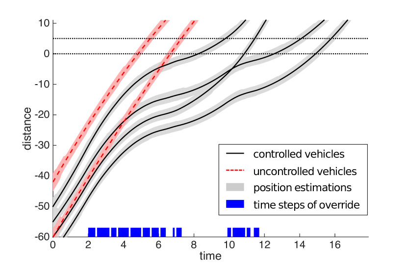
5 Approximate solutions

5.1 Efficient Verification

While scheduling problems on a single machine with arbitrary release times, deadlines, and process times are known to be NP-hard, Garey et al. (1981) proved that the complexity can be reduced to O(nlogn)𝑂𝑛𝑛O(n\log n) if process times of all jobs are identical. This was done using “forbidden regions” and the “earliest deadline scheduling (EDD)” rule. Forbidden regions are time intervals during which no feasible job is allowed to start, and can be computed in O(nlogn)𝑂𝑛𝑛O(n\log n) time. Once forbidden regions are computed, EDD can be used to solve the scheduling problem in O(nlogn)𝑂𝑛𝑛O(n\log n) time.

We design Algorithm 3 by modifying Garey’s result to handle inserted idle-times. We define initial forbidden regions 𝐅0subscript𝐅0\mathbf{F}_{0} to account for the idle-times and set them as inputs of Algorithm 3. In Garey’s result, forbidden regions are initially declared empty and not taken as inputs.

In the procedure in Algorithm 3, rj,djsubscript𝑟𝑗subscript𝑑𝑗r_{j},d_{j}, and tjsubscript𝑡𝑗t_{j} denote the j𝑗j-th entry of 𝐫,𝐝𝐫𝐝\mathbf{r},\mathbf{d}, and 𝐭𝐭\mathbf{t}, respectively, and F0,γsubscript𝐹0𝛾F_{0,\gamma} the γ𝛾\gamma-th interval of 𝐅0subscript𝐅0\mathbf{F}_{0} so that 𝐅0=γF0,γsubscript𝐅0subscript𝛾subscript𝐹0𝛾\mathbf{F}_{0}=\cup_{\gamma}F_{0,\gamma}. Critical time c𝑐c is the latest time at which a job can start at each iteration. A set 𝒜𝒜\mathcal{A} contains jobs that have not been scheduled but are ready to be scheduled at time s𝑠s, which means their release times are smaller than or equal to s𝑠s. A set \mathcal{B} contains all jobs that have not been yet scheduled. Initially, ={1,,|𝐫|}1𝐫\mathcal{B}=\{1,\ldots,|\mathbf{r}|\} where |𝐫|𝐫|\mathbf{r}| is the cardinality of 𝐫𝐫\mathbf{r}.

1:procedure Polynomial(𝐫,𝐝,𝐅𝟎𝐫𝐝subscript𝐅0\mathbf{r,d,F_{0}})
2:    Let σ𝜎\sigma be a vector of indexes in an increasing order of 𝐫𝐫\mathbf{r} and 𝐅=𝐅0𝐅subscript𝐅0\mathbf{F}=\mathbf{F}_{0}.
3:    for i=|𝐫|𝑖𝐫i=|\mathbf{r}| to 1 do \triangleright Forbidden Region Declaration
4:       for j{j:djdσi}𝑗conditional-set𝑗subscript𝑑𝑗subscript𝑑subscript𝜎𝑖j\in\{j:d_{j}\geq d_{\sigma_{i}}\} do
5:           if cjsubscript𝑐𝑗c_{j} undefined then cj=djsubscript𝑐𝑗subscript𝑑𝑗c_{j}=d_{j}
6:           else cj=cj1subscript𝑐𝑗subscript𝑐𝑗1c_{j}=c_{j}-1            
7:           if cjFγsubscript𝑐𝑗subscript𝐹𝛾c_{j}\in F_{\gamma} for some γ𝛾\gamma then cj=infFγsubscript𝑐𝑗infimumsubscript𝐹𝛾c_{j}=\inf{F_{\gamma}}                   
8:       if σi=1subscript𝜎𝑖1\sigma_{i}=1 or rσi1<rσisubscript𝑟subscript𝜎𝑖1subscript𝑟subscript𝜎𝑖r_{\sigma_{i-1}}<r_{\sigma_{i}} then
9:           c=min{cj:cjdefined}𝑐:subscript𝑐𝑗subscript𝑐𝑗definedc=\min\{c_{j}:c_{j}~{}\text{defined}\}        
10:       if c<rσi𝑐subscript𝑟subscript𝜎𝑖c<r_{\sigma_{i}} then ans=no𝑎𝑛𝑠𝑛𝑜ans=no       
11:       if rσic<rσi+1subscript𝑟subscript𝜎𝑖𝑐subscript𝑟subscript𝜎𝑖1r_{\sigma_{i}}\leq c<r_{\sigma_{i}}+1 then 𝐅=𝐅(c1,rσi)𝐅𝐅𝑐1subscript𝑟subscript𝜎𝑖\mathbf{F}=\mathbf{F}\cup(c-1,r_{\sigma_{i}})            
12:    s=0,𝒜=,={1,,|𝐫|}formulae-sequence𝑠0formulae-sequence𝒜1𝐫s=0,\mathcal{A}=\emptyset,\mathcal{B}=\{1,\ldots,|\mathbf{r}|\} \triangleright Schedule Generation
13:    while \mathcal{B}\neq\emptyset do
14:       if sFγ𝑠subscript𝐹𝛾s\in{F}_{\gamma} for some γ𝛾\gamma then s=supFγ𝑠supremumsubscript𝐹𝛾s=\sup{F}_{\gamma}        
15:       if 𝒜=𝒜\mathcal{A}=\emptyset then j=argminjrj𝑗subscriptargmin𝑗subscript𝑟𝑗j=\operatorname*{arg\,min}_{j\in\mathcal{B}}r_{j} and tj=rjsubscript𝑡𝑗subscript𝑟𝑗t_{j}=r_{j}
16:       else j=argminj𝒜dj𝑗subscriptargmin𝑗𝒜subscript𝑑𝑗j=\operatorname*{arg\,min}_{j\in\mathcal{A}}d_{j} and tj=ssubscript𝑡𝑗𝑠t_{j}=s        
17:       s=s+1,={j}formulae-sequence𝑠𝑠1𝑗s=s+1,~{}\mathcal{B}=\mathcal{B}\setminus\{j\} and 𝒜={k:rks}𝒜conditional-set𝑘subscript𝑟𝑘𝑠\mathcal{A}=\{k\in\mathcal{B}:r_{k}\geq s\}     
18:    π=superscript𝜋absent\pi^{*}= a vector of indexes in an increasing order of 𝐭𝐭\mathbf{t}
19:    if ans=no𝑎𝑛𝑠𝑛𝑜ans=no then
20:       return (,π,no)superscript𝜋𝑛𝑜(\emptyset,\pi^{*},no)
21:    else return (𝐭,π,yes)𝐭superscript𝜋𝑦𝑒𝑠(\mathbf{t},\pi^{*},yes)     
Algorithm 3 Modified version of the result of Garey et al. (1981)

In the following lemma, we prove that procedure Polynomial in Algorithm 3 solves the IIT scheduling problem with unit process times. This problem is formulated as follows.

Problem 4.

Given 𝐫,𝐝,𝐫¯,𝐩¯𝐫𝐝¯𝐫¯𝐩\mathbf{r,d,\bar{r},\bar{p}}, determine the existence of a schedule 𝐭𝐭\mathbf{t} satisfying

for allj,for all𝑗\displaystyle\text{for all}~{}j, tj[rj,dj],subscript𝑡𝑗subscript𝑟𝑗subscript𝑑𝑗\displaystyle t_{j}\in[r_{j},d_{j}], (19)
for allij,for all𝑖𝑗\displaystyle\text{for all}~{}i\neq j, (ti,ti+1)(tj,tj+1)=,subscript𝑡𝑖subscript𝑡𝑖1subscript𝑡𝑗subscript𝑡𝑗1\displaystyle(t_{i},t_{i}+1)\cap(t_{j},t_{j}+1)=\emptyset, (20)
for alljandγ,for all𝑗and𝛾\displaystyle\text{for all}~{}j~{}\text{and}~{}\gamma, (tj,tj+1)(r¯γ,p¯γ)=,subscript𝑡𝑗subscript𝑡𝑗1subscript¯𝑟𝛾subscript¯𝑝𝛾\displaystyle(t_{j},t_{j}+1)\cap(\bar{r}_{\gamma},\bar{p}_{\gamma})=\emptyset, (21)

where (r¯γ,p¯γ)subscript¯𝑟𝛾subscript¯𝑝𝛾(\bar{r}_{\gamma},\bar{p}_{\gamma}) denotes the γ𝛾\gamma-th inserted idle-time.

Lemma 1.

Procedure Polynomial in Algorithm 3 solves the IIT scheduling problem with unit process times and finds a feasible schedule if exists.

The proof of Lemma 1 is provided in Appendix B.

To use Algorithm 3, we assign a time interval of equal length to cross the intersection to all vehicles, and formulate a relaxed IIT scheduling problem. The identical process time θmaxsubscript𝜃𝑚𝑎𝑥\theta_{max} is defined as follows:

θmax:=maxj𝒞maxRjTjDjPj(Tj).assignsubscript𝜃𝑚𝑎𝑥subscript𝑗𝒞subscriptsubscript𝑅𝑗subscript𝑇𝑗subscript𝐷𝑗subscript𝑃𝑗subscript𝑇𝑗\theta_{max}:=\max_{j\in\mathcal{C}}\max_{R_{j}\leq T_{j}\leq D_{j}}P_{j}(T_{j}). (22)

Here, θmaxsubscript𝜃𝑚𝑎𝑥\theta_{max} is the maximum time that any controlled vehicle spends crossing an intersection, so that θmaxPj(Tj)subscript𝜃𝑚𝑎𝑥subscript𝑃𝑗subscript𝑇𝑗\theta_{max}\geq P_{j}(T_{j}) for all j𝒞𝑗𝒞j\in\mathcal{C} for any Tj[Rj,Dj]subscript𝑇𝑗subscript𝑅𝑗subscript𝐷𝑗T_{j}\in[R_{j},D_{j}]. In other words, all controlled vehicles are guaranteed to cross the intersection within θmaxsubscript𝜃𝑚𝑎𝑥\theta_{max}.

By replacing Pj(Tj)subscript𝑃𝑗subscript𝑇𝑗P_{j}(T_{j}) in Problem 3 with θmaxsubscript𝜃𝑚𝑎𝑥\theta_{max}, the relaxed IIT scheduling problem is formulated as follows.

Problem 5 ((Relaxed IIT scheduling)).

Given an initial state estimation [𝐱a(0),𝐱b(0)]superscript𝐱𝑎0superscript𝐱𝑏0[\mathbf{x}^{a}(0),\mathbf{x}^{b}(0)], determine whether there exists a schedule 𝐓=(T1,,Tnc)+nc𝐓subscript𝑇1subscript𝑇subscript𝑛𝑐subscriptsuperscriptsubscript𝑛𝑐\mathbf{T}=(T_{1},\ldots,T_{n_{c}})\in\mathbb{R}^{n_{c}}_{+} such that for all j𝒞𝑗𝒞j\in\mathcal{C},

RjTjDj,subscript𝑅𝑗subscript𝑇𝑗subscript𝐷𝑗R_{j}\leq T_{j}\leq D_{j}, (23)

for all ij𝒞𝑖𝑗𝒞i\neq j\in\mathcal{C} if Ti,Tj>0subscript𝑇𝑖subscript𝑇𝑗0T_{i},T_{j}>0,

(Ti,Ti+θmax)(Tj,Tj+θmax)=,subscript𝑇𝑖subscript𝑇𝑖subscript𝜃𝑚𝑎𝑥subscript𝑇𝑗subscript𝑇𝑗subscript𝜃𝑚𝑎𝑥(T_{i},T_{i}+\theta_{max})\cap(T_{j},T_{j}+\theta_{max})=\emptyset, (24)

for all j𝒞𝑗𝒞j\in\mathcal{C} and γ𝒞¯𝛾¯𝒞\gamma\in\bar{\mathcal{C}} if Tj>0subscript𝑇𝑗0T_{j}>0,

(Tj,Tj+θmax)(R¯γ,P¯γ)=.subscript𝑇𝑗subscript𝑇𝑗subscript𝜃𝑚𝑎𝑥subscript¯𝑅𝛾subscript¯𝑃𝛾(T_{j},T_{j}+\theta_{max})\cap(\bar{R}_{\gamma},\bar{P}_{\gamma})=\emptyset. (25)

If Tj=0subscript𝑇𝑗0T_{j}=0, (0,Pj(0))0subscript𝑃𝑗0(0,P_{j}(0)) replaces (Tj,Tj+θmax)subscript𝑇𝑗subscript𝑇𝑗subscript𝜃𝑚𝑎𝑥(T_{j},T_{j}+\theta_{max}) in conditions (24) and (25).

The following algorithm solves this problem by employing Polynomial. This is an exact solution for Problem 5 by Lemma 1. At line 7, we call 𝟎0\mathbf{0} the zero vector in ncsuperscriptsubscript𝑛𝑐\mathbb{R}^{n_{c}}.

1:procedure RelaxedExact([𝐱a(0),𝐱b(0)],Ssuperscript𝐱𝑎0superscript𝐱𝑏0𝑆[\mathbf{x}^{a}(0),\mathbf{x}^{b}(0)],S)
2:    if [𝐲a(0),𝐲b(0)]Bsuperscript𝐲𝑎0superscript𝐲𝑏0𝐵[\mathbf{y}^{a}(0),\mathbf{y}^{b}(0)]\cap B\neq\emptyset then return (,,no)𝑛𝑜(\emptyset,\emptyset,no)     
3:    for all j𝒞𝑗𝒞j\in\mathcal{C} do calculate Rj,Dj,θmaxsubscript𝑅𝑗subscript𝐷𝑗subscript𝜃𝑚𝑎𝑥R_{j},D_{j},\theta_{max}     
4:    for all γ𝒞¯𝛾¯𝒞\gamma\in\bar{\mathcal{C}} do calculate R¯γ,P¯γsubscript¯𝑅𝛾subscript¯𝑃𝛾\bar{R}_{\gamma},\bar{P}_{\gamma}
5:       Fγ=(max(R¯γ/θmax1,0),P¯γ/θmax)subscript𝐹𝛾subscript¯𝑅𝛾subscript𝜃𝑚𝑎𝑥10subscript¯𝑃𝛾subscript𝜃𝑚𝑎𝑥F_{\gamma}=(\max(\bar{R}_{\gamma}/\theta_{max}-1,0),\bar{P}_{\gamma}/\theta_{max})     
6:    ={j𝒞:yjb(0)<αj}conditional-set𝑗𝒞subscriptsuperscript𝑦𝑏𝑗0subscript𝛼𝑗\mathcal{M}=\{j\in\mathcal{C}:y^{b}_{j}(0)<\alpha_{j}\} and ¯=𝒞¯𝒞\bar{\mathcal{M}}=\mathcal{C}\setminus\mathcal{M}
7:    if ||=00|\mathcal{M}|=0 then return (,𝟎,yes)0𝑦𝑒𝑠(\emptyset,\mathbf{0},yes)     
8:    Tj=0subscript𝑇𝑗0T_{j}=0 for all j¯𝑗¯j\in\bar{\mathcal{M}} and Pmax=maxj¯Pj(Tj)subscript𝑃𝑚𝑎𝑥subscript𝑗¯subscript𝑃𝑗subscript𝑇𝑗P_{max}=\max_{j\in\bar{\mathcal{M}}}P_{j}(T_{j})
9:    for all j𝑗j\in{\mathcal{M}} do
10:       rj=max(Rj,Pmax)/θmaxsubscript𝑟𝑗subscript𝑅𝑗subscript𝑃𝑚𝑎𝑥subscript𝜃𝑚𝑎𝑥r_{j}=\max(R_{j},P_{max})/\theta_{max} and dj=Dj/θmaxsubscript𝑑𝑗subscript𝐷𝑗subscript𝜃𝑚𝑎𝑥d_{j}=D_{j}/\theta_{max}     
11:    (𝐭,π,ans)=Polynomial(𝐫,𝐝,𝐅)𝐭superscript𝜋𝑎𝑛𝑠Polynomial𝐫𝐝𝐅(\mathbf{t},\pi^{*},ans)=\textsc{Polynomial}(\mathbf{r,d,F})
12:    if ans=yes𝑎𝑛𝑠𝑦𝑒𝑠ans=yes then Tj=tjθmax,jformulae-sequencesubscript𝑇𝑗subscript𝑡𝑗subscript𝜃𝑚𝑎𝑥for-all𝑗T_{j}=t_{j}\theta_{max},\forall j\in{\mathcal{M}}
13:       return (𝐓,π,yes)𝐓superscript𝜋𝑦𝑒𝑠(\mathbf{T},\pi^{*},yes)
14:    else  return (,π,no)superscript𝜋𝑛𝑜(\emptyset,\pi^{*},no)     
Algorithm 4 Exact Solution of Problem 5

In this procedure, all parameters are normalized by θmaxsubscript𝜃𝑚𝑎𝑥\theta_{max} because procedure Polynomial assumes unit process times. In line 5, the idle-time (R¯γ,P¯γ)subscript¯𝑅𝛾subscript¯𝑃𝛾(\bar{R}_{\gamma},\bar{P}_{\gamma}) is translated into an initial set of forbidden regions Fγsubscript𝐹𝛾F_{\gamma} so that condition (25) is equivalent to tjFγsubscript𝑡𝑗subscript𝐹𝛾t_{j}\notin F_{\gamma}. If tjFγsubscript𝑡𝑗subscript𝐹𝛾t_{j}\in F_{\gamma}, then Tj(max(R¯γθmax,0),P¯γ)subscript𝑇𝑗subscript¯𝑅𝛾subscript𝜃𝑚𝑎𝑥0subscript¯𝑃𝛾T_{j}\in(\max(\bar{R}_{\gamma}-\theta_{max},0),\bar{P}_{\gamma}) so that either Tj(R¯γ,P¯γ)subscript𝑇𝑗subscript¯𝑅𝛾subscript¯𝑃𝛾T_{j}\in(\bar{R}_{\gamma},\bar{P}_{\gamma}) or Tj+θmax(R¯γ,P¯γ)subscript𝑇𝑗subscript𝜃𝑚𝑎𝑥subscript¯𝑅𝛾subscript¯𝑃𝛾T_{j}+\theta_{max}\in(\bar{R}_{\gamma},\bar{P}_{\gamma}).

The running time of procedure RelaxedExact is dominated by Polynomial in line 11, which has an asymptotic running time of O(nc2)𝑂superscriptsubscript𝑛𝑐2O(n_{c}^{2}).

By exploiting procedure RelaxedExact in Algorithm 4, we design a new procedure, called Approx, that solves Problem 2 within an approximation bound. This procedure schedules vehicles according to a sequence returned by procedure RelaxedExact, thereby inheriting computational efficiency. This sequence is denoted by πsuperscript𝜋\pi^{*} in the following algorithm.

1:procedure Approx([𝐱a(0),𝐱b(0)],Ssuperscript𝐱𝑎0superscript𝐱𝑏0𝑆[\mathbf{x}^{a}(0),\mathbf{x}^{b}(0)],S)
2:    if [𝐲a(0),𝐲b(0)]Bsuperscript𝐲𝑎0superscript𝐲𝑏0𝐵[\mathbf{y}^{a}(0),\mathbf{y}^{b}(0)]\cap B\neq\emptyset then return (,no)𝑛𝑜(\emptyset,no)     
3:    if yjb(0)αjsubscriptsuperscript𝑦𝑏𝑗0subscript𝛼𝑗y^{b}_{j}(0)\geq\alpha_{j} for all j𝒞𝑗𝒞j\in\mathcal{C} then return (,yes)𝑦𝑒𝑠(\emptyset,yes)     
4:    (,π,)=RelaxedExact([𝐱a(0),𝐱b(0)],S)superscript𝜋RelaxedExactsuperscript𝐱𝑎0superscript𝐱𝑏0𝑆(\cdot,\pi^{*},\cdot)=\textsc{RelaxedExact}([\mathbf{x}^{a}(0),\mathbf{x}^{b}(0)],S)
5:    (𝐓,ans)=Scheduling(π,[𝐱a(0),𝐱b(0)],S)𝐓𝑎𝑛𝑠Schedulingsuperscript𝜋superscript𝐱𝑎0superscript𝐱𝑏0𝑆(\mathbf{T},ans)=\textsc{Scheduling}(\pi^{*},[\mathbf{x}^{a}(0),\mathbf{x}^{b}(0)],S)
Algorithm 5 Approximate Solution of Problem 3

Procedure Approx in Algorithm 5 trades exactness for computational efficiency. We will prove that procedure Approx is more conservative than procedure Exact, that is, there exists an instance I=([𝐱a(0),𝐱b(0)],S)𝐼superscript𝐱𝑎0superscript𝐱𝑏0𝑆I=([\mathbf{x}^{a}(0),\mathbf{x}^{b}(0)],S) such that Approx(I)𝐼(I) returns no while Exact(I)𝐼(I) returns yes. In order to quantify the degree of conservatism, we prove two theorems. The first theorem states that if procedure Approx returns yes, then there exists an input signal to avoid the Bad set. In the second theorem, if procedure Approx returns no, then there does not exist an input signal to avoid an inflated Bad set, which accounts for the conservatism.

Theorem 3.

If Approx([𝐱a(0),𝐱b(0)],S)=(𝐓,yes)superscript𝐱𝑎0superscript𝐱𝑏0𝑆𝐓𝑦𝑒𝑠([\mathbf{x}^{a}(0),\mathbf{x}^{b}(0)],S)=(\mathbf{T},yes), then ([𝐱a(0),𝐱b(0)],S)superscript𝐱𝑎0superscript𝐱𝑏0𝑆absent([\mathbf{x}^{a}(0),\mathbf{x}^{b}(0)],S)\in Problem 2.

Proof.

By Theorem 1, we only need to show that ([𝐱a(0),𝐱b(0)],S)superscript𝐱𝑎0superscript𝐱𝑏0𝑆absent([\mathbf{x}^{a}(0),\mathbf{x}^{b}(0)],S)\in Problem 3. Notice that procedure Approx of Algorithm 5 returns yes in the case of line 3. In this case, ([𝐱a(0),𝐱b(0)],S)superscript𝐱𝑎0superscript𝐱𝑏0𝑆absent([\mathbf{x}^{a}(0),\mathbf{x}^{b}(0)],S)\in Problem 3 since all vehicles have already crossed the intersection. The procedure also returns yes when procedure Scheduling given a sequence πsuperscript𝜋\pi^{*} returns yes in line 5. Since π𝒫superscript𝜋𝒫\pi^{*}\in\mathcal{P}, where 𝒫𝒫\mathcal{P} is a set of all permutations, and πsuperscript𝜋\pi^{*} yields a feasible schedule, we know Exact([𝐱a(0),𝐱b(0)],S)superscript𝐱𝑎0superscript𝐱𝑏0𝑆([\mathbf{x}^{a}(0),\mathbf{x}^{b}(0)],S) returns yes. Thus, ([𝐱a(0),𝐱b(0)],S)superscript𝐱𝑎0superscript𝐱𝑏0𝑆absent([\mathbf{x}^{a}(0),\mathbf{x}^{b}(0)],S)\in Problem 3. ∎

However, the converse of Theorem 3 is not true. That is, for some instances such that ([𝐱a(0),𝐱b(0)],S)superscript𝐱𝑎0superscript𝐱𝑏0𝑆absent([\mathbf{x}^{a}(0),\mathbf{x}^{b}(0)],S)\in Problem 2, procedure Approx can return no. To consider these instances, we introduce an inflated Bad set.

The IIT scheduling problem finds a schedule satisfying yjb(Tj)=αjsuperscriptsubscript𝑦𝑗𝑏subscript𝑇𝑗subscript𝛼𝑗y_{j}^{b}(T_{j})=\alpha_{j} and yja(Tj+Pj(Tj))=βjsuperscriptsubscript𝑦𝑗𝑎subscript𝑇𝑗subscript𝑃𝑗subscript𝑇𝑗subscript𝛽𝑗y_{j}^{a}(T_{j}+P_{j}(T_{j}))=\beta_{j} for j𝒞𝑗𝒞j\in\mathcal{C}. In contrast, the relaxed IIT scheduling problem finds a schedule satisfying yjb(Tj)=αjsuperscriptsubscript𝑦𝑗𝑏subscript𝑇𝑗subscript𝛼𝑗y_{j}^{b}(T_{j})=\alpha_{j} and yja(Tj+θmax)βjsuperscriptsubscript𝑦𝑗𝑎subscript𝑇𝑗subscript𝜃𝑚𝑎𝑥subscript𝛽𝑗y_{j}^{a}(T_{j}+\theta_{max})\geq{\beta}_{j}. Given that the farthest distance that controlled vehicle j𝑗j can travel during θmaxsubscript𝜃𝑚𝑎𝑥\theta_{max} is θmaxvj,maxsubscript𝜃𝑚𝑎𝑥subscript𝑣𝑗𝑚𝑎𝑥\theta_{max}v_{j,max}, we define an “inflated” intersection (αj,β^j)subscript𝛼𝑗subscript^𝛽𝑗(\alpha_{j},\hat{\beta}_{j}) such that β^j:=αj+θmaxvj,maxassignsubscript^𝛽𝑗subscript𝛼𝑗subscript𝜃𝑚𝑎𝑥subscript𝑣𝑗𝑚𝑎𝑥\hat{\beta}_{j}:=\alpha_{j}+\theta_{max}v_{j,max}. Notice that βjβ^jsubscript𝛽𝑗subscript^𝛽𝑗\beta_{j}\leq\hat{\beta}_{j}. Because the process times are only defined for controlled vehicles, β^γ=βγsubscript^𝛽𝛾subscript𝛽𝛾\hat{\beta}_{\gamma}=\beta_{\gamma} for γ𝒞¯𝛾¯𝒞\gamma\in\bar{\mathcal{C}}. Thus, inflated Bad set B^^𝐵\hat{B} is defined as follows:

B^:={𝐲Y:yi(αi,β^i)andyj(αj,β^j)for someijsuch thati𝒞𝒞¯andj𝒞}.assign^𝐵conditional-set𝐲𝑌subscript𝑦𝑖subscript𝛼𝑖subscript^𝛽𝑖andsubscript𝑦𝑗subscript𝛼𝑗subscript^𝛽𝑗for some𝑖𝑗such that𝑖𝒞¯𝒞and𝑗𝒞\displaystyle\begin{split}\hat{B}:=\{&\mathbf{y}\in Y:y_{i}\in(\alpha_{i},\hat{\beta}_{i})~{}\text{and}~{}y_{j}\in(\alpha_{j},\hat{\beta}_{j})\\ &\text{for some}~{}i\neq j~{}\text{such that}~{}i\in\mathcal{\mathcal{C}\cup\bar{\mathcal{C}}}~{}\text{and}~{}j\in\mathcal{C}\}.\end{split} (26)

By replacing Bad set B𝐵B in Problem 2 with inflated Bad set B^^𝐵\hat{B}, we can formulate the relaxed verification problem. The following theorem is a key result that shows the approximation bound of procedure Approx.

Lemma 2.

If Approx([𝐱a(0),𝐱b(0)],S)=(𝐓,yes)superscript𝐱𝑎0superscript𝐱𝑏0𝑆𝐓𝑦𝑒𝑠([\mathbf{x}^{a}(0),\mathbf{x}^{b}(0)],S)=(\mathbf{T},yes), and RelaxedExact([𝐱a(0),𝐱b(0)],S)=(𝐓¯,π,yes)superscript𝐱𝑎0superscript𝐱𝑏0𝑆¯𝐓superscript𝜋𝑦𝑒𝑠([\mathbf{x}^{a}(0),\mathbf{x}^{b}(0)],S)=(\bar{\mathbf{T}},\pi^{*},yes), then TjT¯jsubscript𝑇𝑗subscript¯𝑇𝑗T_{j}\leq\bar{T}_{j} for all j𝒞𝑗𝒞j\in\mathcal{C}.

Lemma 3.

If Approx([𝐱a(0),𝐱b(0)],S)=(,no)superscript𝐱𝑎0superscript𝐱𝑏0𝑆𝑛𝑜([\mathbf{x}^{a}(0),\mathbf{x}^{b}(0)],S)=(\emptyset,no), then RelaxedExact([𝐱a(0),𝐱b(0)],S)=(,π,no)superscript𝐱𝑎0superscript𝐱𝑏0𝑆superscript𝜋𝑛𝑜([\mathbf{x}^{a}(0),\mathbf{x}^{b}(0)],S)=(\emptyset,\pi^{*},no).

The proofs of Lemmas 2 and 3 can be found in Appendix B.

Theorem 4.

If Approx([𝐱a(0),𝐱b(0)],S)=(,no)superscript𝐱𝑎0superscript𝐱𝑏0𝑆𝑛𝑜([\mathbf{x}^{a}(0),\mathbf{x}^{b}(0)],S)=(\emptyset,no), then there is no input signal 𝐮()𝐮\mathbf{u}(\cdot) that guarantees 𝐲(t,𝐮(),𝐰(),𝐝(),𝐱(0))B^𝐲𝑡𝐮𝐰𝐝𝐱0^𝐵\mathbf{y}(t,\mathbf{u}(\cdot),\mathbf{w}(\cdot),\mathbf{d}(\cdot),\mathbf{x}(0))\notin\hat{B} for all t0𝑡0t\geq 0 for any 𝐰()𝒲,𝐝()𝒟,formulae-sequence𝐰𝒲𝐝𝒟\mathbf{w}(\cdot)\in\mathcal{W},\mathbf{d}(\cdot)\in\mathcal{D}, and 𝐱(0)[𝐱a(0),𝐱b(0)]𝐱0superscript𝐱𝑎0superscript𝐱𝑏0\mathbf{x}(0)\in[\mathbf{x}^{a}(0),\mathbf{x}^{b}(0)].

Algorithm 6 Implementation of sesubscript𝑠𝑒s_{e}
1:procedure EffSupervisor([𝐱a(kτ),𝐱b(kτ)],𝐮desireksuperscript𝐱𝑎𝑘𝜏superscript𝐱𝑏𝑘𝜏superscriptsubscript𝐮𝑑𝑒𝑠𝑖𝑟𝑒𝑘[\mathbf{x}^{a}(k\tau),\mathbf{x}^{b}(k\tau)],\mathbf{u}_{desire}^{k})
2:    (𝐓1,ans1)=Approx(𝐗pred(𝐮desirek()),S)subscript𝐓1𝑎𝑛subscript𝑠1Approxsubscript𝐗𝑝𝑟𝑒𝑑superscriptsubscript𝐮𝑑𝑒𝑠𝑖𝑟𝑒𝑘𝑆(\mathbf{T}_{1},ans_{1})=\textsc{Approx}(\mathbf{X}_{pred}(\mathbf{u}_{desire}^{k}(\cdot)),S)
3:    if ans1=yes𝑎𝑛subscript𝑠1𝑦𝑒𝑠ans_{1}=yes and for all t[0,τ),B[𝐱a(t,𝐮desirek(),𝐱a(kτ)),𝐱b(t,𝐮desirek(),𝐱b(kτ))]=formulae-sequence𝑡0𝜏𝐵superscript𝐱𝑎𝑡superscriptsubscript𝐮𝑑𝑒𝑠𝑖𝑟𝑒𝑘superscript𝐱𝑎𝑘𝜏superscript𝐱𝑏𝑡superscriptsubscript𝐮𝑑𝑒𝑠𝑖𝑟𝑒𝑘superscript𝐱𝑏𝑘𝜏t\in[0,\tau),B\cap[\mathbf{x}^{a}(t,\mathbf{u}_{desire}^{k}(\cdot),\mathbf{x}^{a}(k\tau)),\mathbf{x}^{b}(t,\mathbf{u}_{desire}^{k}(\cdot),\mathbf{x}^{b}(k\tau))]=\emptyset  then
4:       πk=superscript𝜋𝑘absent\pi^{k}= a vector of indexes in the increasing order of nonzero entries of 𝐓1subscript𝐓1\mathbf{T}_{1}
5:       𝐮safek+1,()=σ(𝐗pred(𝐮desirek()),𝐓1)subscriptsuperscript𝐮𝑘1𝑠𝑎𝑓𝑒𝜎subscript𝐗𝑝𝑟𝑒𝑑superscriptsubscript𝐮𝑑𝑒𝑠𝑖𝑟𝑒𝑘subscript𝐓1\mathbf{u}^{{k+1,\infty}}_{safe}(\cdot)=\sigma(\mathbf{X}_{pred}(\mathbf{u}_{desire}^{k}(\cdot)),\mathbf{T}_{1})
6:       𝐮safek+1()=𝐮safek+1,(t)fort[(k+1)τ,(k+2)τ)subscriptsuperscript𝐮𝑘1𝑠𝑎𝑓𝑒superscriptsubscript𝐮𝑠𝑎𝑓𝑒𝑘1𝑡for𝑡𝑘1𝜏𝑘2𝜏\mathbf{u}^{{k+1}}_{safe}(\cdot)=\mathbf{u}_{safe}^{k+1,\infty}(t)~{}\text{for}~{}t\in[(k+1)\tau,(k+2)\tau)
7:       return 𝐮desirek()superscriptsubscript𝐮𝑑𝑒𝑠𝑖𝑟𝑒𝑘\mathbf{u}_{desire}^{k}(\cdot)
8:    else
9:       (𝐓2,ans2)=Approx(𝐗pred(𝐮safek()),S)subscript𝐓2𝑎𝑛subscript𝑠2Approxsubscript𝐗𝑝𝑟𝑒𝑑subscriptsuperscript𝐮𝑘𝑠𝑎𝑓𝑒𝑆(\mathbf{T}_{2},ans_{2})=\textsc{Approx}(\mathbf{X}_{pred}(\mathbf{u}^{{k}}_{safe}(\cdot)),S)
10:       if ans2=no𝑎𝑛subscript𝑠2𝑛𝑜ans_{2}=no then
11:           (𝐓2,ans3)=Scheduling(πk1,𝐗pred(𝐮safek()),S)subscript𝐓2𝑎𝑛subscript𝑠3Schedulingsuperscript𝜋𝑘1subscript𝐗𝑝𝑟𝑒𝑑subscriptsuperscript𝐮𝑘𝑠𝑎𝑓𝑒𝑆(\mathbf{T}_{2},ans_{3})=\textsc{Scheduling}(\pi^{k-1},\mathbf{X}_{pred}(\mathbf{u}^{{k}}_{safe}(\cdot)),S)        
12:       πk=superscript𝜋𝑘absent\pi^{k}= a vector of indexes in the increasing order of nonzero entries of 𝐓2subscript𝐓2\mathbf{T}_{2}
13:       𝐮safek+1,()=σ(𝐗pred(𝐮safek()),𝐓2)subscriptsuperscript𝐮𝑘1𝑠𝑎𝑓𝑒𝜎subscript𝐗𝑝𝑟𝑒𝑑subscriptsuperscript𝐮𝑘𝑠𝑎𝑓𝑒subscript𝐓2\mathbf{u}^{{k+1,\infty}}_{safe}(\cdot)=\sigma(\mathbf{X}_{pred}(\mathbf{u}^{{k}}_{safe}(\cdot)),\mathbf{T}_{2})
14:       𝐮safek+1()=𝐮safek+1,(t)fort[(k+1)τ,(k+2)τ)subscriptsuperscript𝐮𝑘1𝑠𝑎𝑓𝑒superscriptsubscript𝐮𝑠𝑎𝑓𝑒𝑘1𝑡for𝑡𝑘1𝜏𝑘2𝜏\mathbf{u}^{{k+1}}_{safe}(\cdot)=\mathbf{u}_{safe}^{k+1,\infty}(t)~{}\text{for}~{}t\in[(k+1)\tau,(k+2)\tau)
15:       return 𝐮safek()subscriptsuperscript𝐮𝑘𝑠𝑎𝑓𝑒\mathbf{u}^{{k}}_{safe}(\cdot)     
Proof.

By Lemma 3, Approx([𝐱a(0),𝐱b(0)],S)=(,no)superscript𝐱𝑎0superscript𝐱𝑏0𝑆𝑛𝑜([\mathbf{x}^{a}(0),\mathbf{x}^{b}(0)],S)=(\emptyset,no) means that RelaxedExact returns no. Thus, we will prove that if there is no schedule satisfying conditions (23)-(25), there is no input signal to avoid the inflated Bad set for any uncertainty. For ease of proof, we prove the contrapositive statement. That is, assume that there is an input signal 𝐮~()𝒰~𝐮𝒰\mathbf{\tilde{u}}(\cdot)\in\mathcal{U} such that 𝐲(t,𝐮~(),𝐰(),𝐝(),𝐱(0))B^𝐲𝑡~𝐮𝐰𝐝𝐱0^𝐵\mathbf{y}(t,\mathbf{\tilde{u}}(\cdot),\mathbf{w}(\cdot),\mathbf{d}(\cdot),\mathbf{x}(0))\notin\hat{B} for all t𝑡t for any 𝐰()𝒲,𝐝()𝒟formulae-sequence𝐰𝒲𝐝𝒟\mathbf{w}(\cdot)\in\mathcal{W},~{}\mathbf{d}(\cdot)\in\mathcal{D}, and 𝐱(0)[𝐱a(0),𝐱b(0)]𝐱0superscript𝐱𝑎0superscript𝐱𝑏0\mathbf{x}(0)\in[\mathbf{x}^{a}(0),\mathbf{x}^{b}(0)]. Then, there exists schedule 𝐓~~𝐓\tilde{\mathbf{T}} satisfying conditions (23)-(25). This proof is similar to the first part of the proof of Theorem 1.

For all j𝒞𝑗𝒞j\in\mathcal{C}, define T~jsubscript~𝑇𝑗\tilde{T}_{j} as yjb(T~j,u~j(),xjb(0))=αjsubscriptsuperscript𝑦𝑏𝑗subscript~𝑇𝑗subscript~𝑢𝑗subscriptsuperscript𝑥𝑏𝑗0subscript𝛼𝑗y^{b}_{j}(\tilde{T}_{j},{\tilde{u}}_{j}(\cdot),x^{b}_{j}(0))=\alpha_{j} if yjb(0)<αjsubscriptsuperscript𝑦𝑏𝑗0subscript𝛼𝑗y^{b}_{j}(0)<\alpha_{j}, and 00 otherwise, and K~jsubscript~𝐾𝑗\tilde{K}_{j} as yja(K~j,u~j(),xja(0))=β^jsubscriptsuperscript𝑦𝑎𝑗subscript~𝐾𝑗subscript~𝑢𝑗subscriptsuperscript𝑥𝑎𝑗0subscript^𝛽𝑗y^{a}_{j}(\tilde{K}_{j},{\tilde{u}}_{j}(\cdot),x^{a}_{j}(0))=\hat{\beta}_{j} if yja(0)<β^jsubscriptsuperscript𝑦𝑎𝑗0subscript^𝛽𝑗y^{a}_{j}(0)<\hat{\beta}_{j}, and 00 otherwise. For ij𝒞𝑖𝑗𝒞i\neq j\in\mathcal{C}, since yi(t,u~i(),di(),xi(0))subscript𝑦𝑖𝑡subscript~𝑢𝑖subscript𝑑𝑖subscript𝑥𝑖0y_{i}(t,{\tilde{u}}_{i}(\cdot),{d}_{i}(\cdot),x_{i}(0)) and yj(t,u~j(),dj(),xj(0))subscript𝑦𝑗𝑡subscript~𝑢𝑗subscript𝑑𝑗subscript𝑥𝑗0y_{j}(t,{\tilde{u}}_{j}(\cdot),{d}_{j}(\cdot),x_{j}(0)) avoid the inflated Bad set for any 𝐝()𝒟𝐝𝒟\mathbf{d}(\cdot)\in\mathcal{D} and 𝐱(0)[𝐱a(0),𝐱b(0)]𝐱0superscript𝐱𝑎0superscript𝐱𝑏0\mathbf{x}(0)\in[\mathbf{x}^{a}(0),\mathbf{x}^{b}(0)], (T~i,K~i)(T~j,K~j)=subscript~𝑇𝑖subscript~𝐾𝑖subscript~𝑇𝑗subscript~𝐾𝑗(\tilde{T}_{i},\tilde{K}_{i})\cap(\tilde{T}_{j},\tilde{K}_{j})=\emptyset. Since the inflated intersection takes account of the maximum driving distance during θmaxsubscript𝜃𝑚𝑎𝑥\theta_{max}, we have yja(T~j+θmax,u~j(),xa(0))β^jsubscriptsuperscript𝑦𝑎𝑗subscript~𝑇𝑗subscript𝜃𝑚𝑎𝑥subscript~𝑢𝑗superscript𝑥𝑎0subscript^𝛽𝑗y^{a}_{j}(\tilde{T}_{j}+\theta_{max},{\tilde{u}}_{j}(\cdot),x^{a}(0))\leq\hat{\beta}_{j}. This implies T~j+θmaxK~jsubscript~𝑇𝑗subscript𝜃𝑚𝑎𝑥subscript~𝐾𝑗\tilde{T}_{j}+\theta_{max}\leq\tilde{K}_{j} for all j𝒞𝑗𝒞j\in\mathcal{C} because yja(t)superscriptsubscript𝑦𝑗𝑎𝑡y_{j}^{a}(t) is non-decreasing in t𝑡t. Thus, (T~i,T~i+θmax)(T~j,T~j+θmax)=subscript~𝑇𝑖subscript~𝑇𝑖subscript𝜃𝑚𝑎𝑥subscript~𝑇𝑗subscript~𝑇𝑗subscript𝜃𝑚𝑎𝑥(\tilde{T}_{i},\tilde{T}_{i}+\theta_{max})\cap(\tilde{T}_{j},\tilde{T}_{j}+\theta_{max})=\emptyset (condition (24)).

For γ𝒞¯𝛾¯𝒞\gamma\in\bar{\mathcal{C}}, define (R¯γ,P¯γ)subscript¯𝑅𝛾subscript¯𝑃𝛾(\bar{R}_{\gamma},\bar{P}_{\gamma}) as in Definition 2. Then, for any wγ()𝒲γ,dγ()𝒟γ,formulae-sequencesubscript𝑤𝛾subscript𝒲𝛾subscript𝑑𝛾subscript𝒟𝛾{w}_{\gamma}(\cdot)\in\mathcal{W}_{\gamma},{d}_{\gamma}(\cdot)\in\mathcal{D}_{\gamma}, and xγ(0)[xγa(0),xγb(0)]subscript𝑥𝛾0superscriptsubscript𝑥𝛾𝑎0superscriptsubscript𝑥𝛾𝑏0x_{\gamma}(0)\in[x_{\gamma}^{a}(0),x_{\gamma}^{b}(0)], uncontrolled vehicle γ𝛾\gamma enters the intersection no earlier than R¯γsubscript¯𝑅𝛾\bar{R}_{\gamma} and exits it no later than P¯γsubscript¯𝑃𝛾\bar{P}_{\gamma}. In order for u~j()subscript~𝑢𝑗{\tilde{u}}_{j}(\cdot) to guarantee that yj(t,u~j(),dj(),xj(0))subscript𝑦𝑗𝑡subscript~𝑢𝑗subscript𝑑𝑗subscript𝑥𝑗0y_{j}(t,{\tilde{u}}_{j}(\cdot),{d}_{j}(\cdot),x_{j}(0)) and yγ(t)subscript𝑦𝛾𝑡y_{\gamma}(t) never meet inside the intersection for any uncertainty, (T~j,K~j)(R¯γ,P¯γ)=subscript~𝑇𝑗subscript~𝐾𝑗subscript¯𝑅𝛾subscript¯𝑃𝛾(\tilde{T}_{j},\tilde{K}_{j})\cap(\bar{R}_{\gamma},\bar{P}_{\gamma})=\emptyset. Since T~j+θmaxK~jsubscript~𝑇𝑗subscript𝜃𝑚𝑎𝑥subscript~𝐾𝑗\tilde{T}_{j}+\theta_{max}\leq\tilde{K}_{j}, we have (T~j,T~j+θmax)(R¯γ,P¯γ)=subscript~𝑇𝑗subscript~𝑇𝑗subscript𝜃𝑚𝑎𝑥subscript¯𝑅𝛾subscript¯𝑃𝛾(\tilde{T}_{j},\tilde{T}_{j}+\theta_{max})\cap(\bar{R}_{\gamma},\bar{P}_{\gamma})=\emptyset (condition (25)).

Condition (23) is satisfied by the definitions of Rjsubscript𝑅𝑗R_{j} and Djsubscript𝐷𝑗D_{j}. ∎∎

In summary, Theorem 3 states that if procedure Approx returns yes, there exists an input signal to avoid the Bad set B𝐵B for any uncertainty. As stated in Theorem 4, if the procedure returns no, there does not exist an input signal to avoid the inflated Bad set B^^𝐵\hat{B} for any uncertainty. Thus, the difference between B𝐵B and B^^𝐵\hat{B} is a measure of the approximation bound of procedure Approx.

5.2 Efficient supervisor

In order for a supervisor to run in real time, the verification problem must be solved within the time step τ𝜏\tau. However, if a large number of controlled vehicles is considered, the problem becomes intractable. Thus, we employ the results in Section 5.1 to design efficient supervisors. The simplest solution would be to implement a supervisor s^([𝐱a(kτ),𝐱b(kτ)],𝐮desirek)^𝑠superscript𝐱𝑎𝑘𝜏superscript𝐱𝑏𝑘𝜏superscriptsubscript𝐮𝑑𝑒𝑠𝑖𝑟𝑒𝑘\hat{s}([\mathbf{x}^{a}(k\tau),\mathbf{x}^{b}(k\tau)],\mathbf{u}_{desire}^{k}) defined as follows:

s^={𝐮desirek()if𝐮desirek,(): for allt0𝐲(t,𝐮desirek,(),𝐰(),𝐝(),𝐱(kτ))B^𝐮safek()otherwise.^𝑠casessuperscriptsubscript𝐮𝑑𝑒𝑠𝑖𝑟𝑒𝑘:ifsubscriptsuperscript𝐮𝑘𝑑𝑒𝑠𝑖𝑟𝑒 for all𝑡0otherwise𝐲𝑡subscriptsuperscript𝐮𝑘𝑑𝑒𝑠𝑖𝑟𝑒𝐰𝐝𝐱𝑘𝜏^𝐵subscriptsuperscript𝐮𝑘𝑠𝑎𝑓𝑒otherwise.\hat{s}=\begin{cases}\mathbf{u}_{desire}^{k}(\cdot)&\text{if}~{}\exists\mathbf{u}^{{k},\infty}_{desire}(\cdot):\text{ for all}~{}t\geq 0\\ &\mathbf{y}(t,\mathbf{u}^{{k},\infty}_{desire}(\cdot),\mathbf{w}(\cdot),\mathbf{d}(\cdot),\mathbf{x}(k\tau))\notin\hat{B}\\ \mathbf{u}^{{k}}_{safe}(\cdot)&\text{otherwise.}\end{cases}

The only difference from the exact supervisor s𝑠s is that the Bad set B𝐵B is replaced by the inflated Bad set B^^𝐵\hat{B}.

Instead of implementing s^^𝑠\hat{s}, we consider a procedure implementing another supervisor, sesubscript𝑠𝑒s_{e}, by using procedure Approx to verify whether or not to override drivers. We call this procedure EffSupervisor in Algorithm 6.

Notice that this procedure stores the feasible sequence of vehicles crossing the intersection at every time step (lines 4 and 12). This is because when the sequence considered in line 9 does not yield a feasible schedule, the previous step’s sequence πk1superscript𝜋𝑘1\pi^{k-1} can be used to generate one. This is where in procedure Scheduling in Algorithm 1, |π0|subscript𝜋0|\pi_{0}| can be different from |π|𝜋|\pi|, where π0=πk1subscript𝜋0superscript𝜋𝑘1\pi_{0}=\pi^{k-1} and π||𝜋superscript\pi\in\mathbb{R}^{|\mathcal{M}|}. This is because \mathcal{M} is a set of vehicles that have not entered an intersection at the current step, whereas πk1superscript𝜋𝑘1\pi^{k-1} is a sequence of vehicles that had not entered an intersection at the previous step.

The fact that the previous step’s sequence leads to a feasible schedule ensures the non-blocking property of the supervisor and is proved in the next theorem. Bruni et al. (2013) proposed an efficient supervisor considering measurement errors and unmodeled dynamics with all vehicles controlled. Their supervisor cannot find a feasible schedule at every step and thus uses the previous schedule until a new feasible schedule is found. This ignores the correction of the state estimation during the open-loop control, thereby being more conservative than our efficient supervisor, which updates the schedule based on the most current state estimation.

Procedure EffSupervisor takes polynomial computation time, and guarantees avoiding the Bad set B𝐵B because such a safe input exists if procedure Approx returns yes by Theorem 3. Most importantly, we will prove in the following theorem that sesubscript𝑠𝑒s_{e} is less restrictive than s^^𝑠\hat{s}, in the sense that s^^𝑠\hat{s} overrides controlled vehicles more frequently than sesubscript𝑠𝑒s_{e}.

Theorem 5.

The supervisor sesubscript𝑠𝑒s_{e} is less restrictive than s^^𝑠\hat{s}: if EffSupervisor([𝐱a(kτ),𝐱b(kτ)],𝐮desirek)=𝐮safek()superscript𝐱𝑎𝑘𝜏superscript𝐱𝑏𝑘𝜏superscriptsubscript𝐮𝑑𝑒𝑠𝑖𝑟𝑒𝑘subscriptsuperscript𝐮𝑘𝑠𝑎𝑓𝑒([\mathbf{x}^{a}(k\tau),\mathbf{x}^{b}(k\tau)],\mathbf{u}_{desire}^{k})=\mathbf{u}^{{k}}_{safe}(\cdot), then s^([𝐱a(kτ),𝐱b(kτ)],𝐮desirek)=𝐮safek()^𝑠superscript𝐱𝑎𝑘𝜏superscript𝐱𝑏𝑘𝜏superscriptsubscript𝐮𝑑𝑒𝑠𝑖𝑟𝑒𝑘subscriptsuperscript𝐮𝑘𝑠𝑎𝑓𝑒\hat{s}([\mathbf{x}^{a}(k\tau),\mathbf{x}^{b}(k\tau)],\mathbf{u}_{desire}^{k})=\mathbf{u}^{{k}}_{safe}(\cdot). Moreover, sesubscript𝑠𝑒s_{e} is non-blocking.

Proof.

EffSupervisor([𝐱a(kτ),𝐱b(kτ)],𝐮desirek)=𝐮safek()superscript𝐱𝑎𝑘𝜏superscript𝐱𝑏𝑘𝜏superscriptsubscript𝐮𝑑𝑒𝑠𝑖𝑟𝑒𝑘subscriptsuperscript𝐮𝑘𝑠𝑎𝑓𝑒([\mathbf{x}^{a}(k\tau),\mathbf{x}^{b}(k\tau)],\mathbf{u}_{desire}^{k})=\mathbf{u}^{{k}}_{safe}(\cdot) when Approx(𝐗pred(𝐮desirek()),S)subscript𝐗𝑝𝑟𝑒𝑑superscriptsubscript𝐮𝑑𝑒𝑠𝑖𝑟𝑒𝑘𝑆(\mathbf{X}_{pred}(\mathbf{u}_{desire}^{k}(\cdot)),S) returns no. By Theorem 4, there is no input signal 𝐮desirek,()𝒰subscriptsuperscript𝐮𝑘𝑑𝑒𝑠𝑖𝑟𝑒𝒰\mathbf{u}^{{k},\infty}_{desire}(\cdot)\in\mathcal{U} that can prevent entering the inflated Bad set for some uncertainties. Thus, s^(𝐗pred(𝐮desirek),S)^𝑠subscript𝐗𝑝𝑟𝑒𝑑superscriptsubscript𝐮𝑑𝑒𝑠𝑖𝑟𝑒𝑘𝑆\hat{s}(\mathbf{X}_{pred}(\mathbf{u}_{desire}^{k}),S) returns 𝐮safek()subscriptsuperscript𝐮𝑘𝑠𝑎𝑓𝑒\mathbf{u}^{{k}}_{safe}(\cdot). This proves that sesubscript𝑠𝑒s_{e} is less restrictive than s^^𝑠\hat{s}.

The non-blocking property is proved by mathematical induction on time step k𝑘k. For the base case, it is assumed that EffSupervisor([𝐱a(0),𝐱b(0)],𝐮desire0)=𝐮out0()superscript𝐱𝑎0superscript𝐱𝑏0superscriptsubscript𝐮𝑑𝑒𝑠𝑖𝑟𝑒0subscriptsuperscript𝐮0𝑜𝑢𝑡([\mathbf{x}^{a}(0),\mathbf{x}^{b}(0)],\mathbf{u}_{desire}^{0})=\mathbf{u}^{{0}}_{out}(\cdot)\neq\emptyset where 𝐮out0()subscriptsuperscript𝐮0𝑜𝑢𝑡\mathbf{u}^{{0}}_{out}(\cdot) is defined on time [0,τ)0𝜏[0,\tau), and 𝐮safe1,()subscriptsuperscript𝐮1𝑠𝑎𝑓𝑒\mathbf{u}^{{1,\infty}}_{safe}(\cdot) is well-defined, that is, there exists a schedule 𝐓𝐓\mathbf{T} that defines 𝐮safe1,()subscriptsuperscript𝐮1𝑠𝑎𝑓𝑒\mathbf{u}^{{1,\infty}}_{safe}(\cdot) as σ(𝐗pred(𝐮desire0()),𝐓)𝜎subscript𝐗𝑝𝑟𝑒𝑑superscriptsubscript𝐮𝑑𝑒𝑠𝑖𝑟𝑒0𝐓\sigma(\mathbf{X}_{pred}(\mathbf{u}_{desire}^{0}(\cdot)),\mathbf{T}). Suppose at t=(k1)τ𝑡𝑘1𝜏t=(k-1)\tau, we have EffSupervisor([𝐱a((k1)τ),𝐱b((k1)τ)],𝐮desirek1)=𝐮outk1()superscript𝐱𝑎𝑘1𝜏superscript𝐱𝑏𝑘1𝜏superscriptsubscript𝐮𝑑𝑒𝑠𝑖𝑟𝑒𝑘1subscriptsuperscript𝐮𝑘1𝑜𝑢𝑡([\mathbf{x}^{a}((k-1)\tau),\mathbf{x}^{b}((k-1)\tau)],\mathbf{u}_{desire}^{k-1})=\mathbf{u}^{{k-1}}_{out}(\cdot)\neq\emptyset and 𝐮safek,()subscriptsuperscript𝐮𝑘𝑠𝑎𝑓𝑒\mathbf{u}^{{k,\infty}}_{safe}(\cdot) is well-defined, which satisfies 𝐲(t,𝐮safek,(),𝐰(),𝐝(),𝐱(kτ))B𝐲𝑡subscriptsuperscript𝐮𝑘𝑠𝑎𝑓𝑒𝐰𝐝𝐱𝑘𝜏𝐵\mathbf{y}(t,\mathbf{u}^{{k,\infty}}_{safe}(\cdot),\mathbf{w}(\cdot),\mathbf{d}(\cdot),\mathbf{x}(k\tau))\notin B for any 𝐰()𝒲,𝐝()𝒟formulae-sequence𝐰𝒲𝐝𝒟\mathbf{w}(\cdot)\in\mathcal{W},\mathbf{d}(\cdot)\in\mathcal{D}, and 𝐱(kτ)𝐗pred(𝐮outk1())𝐱𝑘𝜏subscript𝐗𝑝𝑟𝑒𝑑subscriptsuperscript𝐮𝑘1𝑜𝑢𝑡\mathbf{x}(k\tau)\in\mathbf{X}_{pred}(\mathbf{u}^{{k-1}}_{out}(\cdot)). Now, we need to prove that 𝐮outk()subscriptsuperscript𝐮𝑘𝑜𝑢𝑡\mathbf{u}^{{k}}_{out}(\cdot)\neq\emptyset, and 𝐮safek+1,()subscriptsuperscript𝐮𝑘1𝑠𝑎𝑓𝑒\mathbf{u}^{{k+1,\infty}}_{safe}(\cdot) is well-defined.

In Algorithm 6, if ans1=yes𝑎𝑛subscript𝑠1𝑦𝑒𝑠ans_{1}=yes in line 2 or ans2=yes𝑎𝑛subscript𝑠2𝑦𝑒𝑠ans_{2}=yes in line 9, by Theorem 3, there exists an input signal that makes the vehicle trajectories avoid entering the Bad set. Thus, 𝐮safek+1,()subscriptsuperscript𝐮𝑘1𝑠𝑎𝑓𝑒\mathbf{u}^{{k+1,\infty}}_{safe}(\cdot) is well-defined on time [(k+1)τ,)𝑘1𝜏[(k+1)\tau,\infty) in lines 5 and 13. Also, 𝐮outk()=subscriptsuperscript𝐮𝑘𝑜𝑢𝑡\mathbf{u}^{{k}}_{out}(\cdot)=\emptyset because 𝐮outk()=𝐮desirek,()subscriptsuperscript𝐮𝑘𝑜𝑢𝑡subscriptsuperscript𝐮𝑘𝑑𝑒𝑠𝑖𝑟𝑒\mathbf{u}^{{k}}_{out}(\cdot)=\mathbf{u}^{{k},\infty}_{desire}(\cdot) or 𝐮outk()=𝐮safek()subscriptsuperscript𝐮𝑘𝑜𝑢𝑡subscriptsuperscript𝐮𝑘𝑠𝑎𝑓𝑒\mathbf{u}^{{k}}_{out}(\cdot)=\mathbf{u}^{{k}}_{safe}(\cdot).

Suppose that ans1=no𝑎𝑛subscript𝑠1𝑛𝑜ans_{1}=no and ans2=no𝑎𝑛subscript𝑠2𝑛𝑜ans_{2}=no. Then, given πk1superscript𝜋𝑘1\pi^{k-1}, we need to prove that ans3=yes𝑎𝑛subscript𝑠3𝑦𝑒𝑠ans_{3}=yes and 𝐓2subscript𝐓2\mathbf{T}_{2} exists in line 11. Notice that πk1superscript𝜋𝑘1\pi^{k-1} is a vector of indexed in the increasing order of the nonzero entries of a feasible schedule 𝐓k1superscript𝐓𝑘1\mathbf{T}^{k-1} of the previous step. That is, at the previous step, Scheduling(πk1,𝐗pred(𝐮outk1()),S)=(𝐓k1,yes)superscript𝜋𝑘1subscript𝐗𝑝𝑟𝑒𝑑subscriptsuperscript𝐮𝑘1𝑜𝑢𝑡𝑆superscript𝐓𝑘1𝑦𝑒𝑠(\pi^{k-1},\mathbf{X}_{pred}(\mathbf{u}^{{k-1}}_{out}(\cdot)),S)=(\mathbf{T}^{k-1},yes). We will show that the existence of 𝐓k1superscript𝐓𝑘1\mathbf{T}^{k-1} implies that of 𝐓2subscript𝐓2\mathbf{T}_{2}.

Let 𝐮safek+1,()subscriptsuperscript𝐮𝑘1𝑠𝑎𝑓𝑒\mathbf{u}^{{k+1,\infty}}_{safe}(\cdot) be 𝐮safek,()subscriptsuperscript𝐮𝑘𝑠𝑎𝑓𝑒\mathbf{u}^{{k,\infty}}_{safe}(\cdot) restricted to time [(k+1)τ,)𝑘1𝜏[(k+1)\tau,\infty) and 𝐮safek()subscriptsuperscript𝐮𝑘𝑠𝑎𝑓𝑒\mathbf{u}^{{k}}_{safe}(\cdot) be 𝐮safek,()subscriptsuperscript𝐮𝑘𝑠𝑎𝑓𝑒\mathbf{u}^{{k,\infty}}_{safe}(\cdot) restricted to time [kτ,(k+1)τ)𝑘𝜏𝑘1𝜏[k\tau,(k+1)\tau). Then, the j𝑗j-th entry of 𝐓k1superscript𝐓𝑘1\mathbf{T}^{k-1} is as follows:

Tjk1:={t:yjb(t,usafe,jk,(),maxXpred,j(uout,jk1()))=αj}assignsuperscriptsubscript𝑇𝑗𝑘1conditional-set𝑡subscriptsuperscript𝑦𝑏𝑗𝑡subscriptsuperscript𝑢𝑘𝑠𝑎𝑓𝑒𝑗subscript𝑋𝑝𝑟𝑒𝑑𝑗superscriptsubscript𝑢𝑜𝑢𝑡𝑗𝑘1subscript𝛼𝑗\displaystyle T_{j}^{k-1}:=\{t:y^{b}_{j}(t,{u}^{{k},\infty}_{safe,{j}}(\cdot),\max X_{pred,j}(u_{out,j}^{k-1}(\cdot)))=\alpha_{j}\}
={t:yjb(t,usafe,jk+1,(),\displaystyle=\{t:y^{b}_{j}(t,{u}^{{k+1},\infty}_{safe,{j}}(\cdot),
xb(τ,usafe,jk(),maxXpred,j(uout,jk1()))=αj}+τ\displaystyle\hskip 36.135ptx^{b}(\tau,u_{safe,j}^{k}(\cdot),\max X_{pred,j}(u_{out,j}^{k-1}(\cdot)))=\alpha_{j}\}+\tau
{t:yjb(t,usafe,jk+1,(),xb(τ,usafe,jk(),xb(kτ)))=αj}+τabsentconditional-set𝑡subscriptsuperscript𝑦𝑏𝑗𝑡subscriptsuperscript𝑢𝑘1𝑠𝑎𝑓𝑒𝑗superscript𝑥𝑏𝜏superscriptsubscript𝑢𝑠𝑎𝑓𝑒𝑗𝑘superscript𝑥𝑏𝑘𝜏subscript𝛼𝑗𝜏\displaystyle\leq\{t:y^{b}_{j}(t,{u}^{{k+1},\infty}_{safe,{j}}(\cdot),x^{b}(\tau,u_{safe,j}^{k}(\cdot),x^{b}(k\tau)))=\alpha_{j}\}+\tau
:=T~j+τ.assignabsentsubscript~𝑇𝑗𝜏\displaystyle:=\tilde{T}_{j}+\tau. (27)

The inequality is due to [xja(kτ),xjb(kτ)]Xpred,j(uout,jk1())subscriptsuperscript𝑥𝑎𝑗𝑘𝜏subscriptsuperscript𝑥𝑏𝑗𝑘𝜏subscript𝑋𝑝𝑟𝑒𝑑𝑗superscriptsubscript𝑢𝑜𝑢𝑡𝑗𝑘1[x^{a}_{j}(k\tau),x^{b}_{j}(k\tau)]\subseteq{X}_{pred,j}(u_{out,j}^{k-1}(\cdot)) by (14) and the order-preserving property in Assumption 1. Similarly, its process time Tjk1+Pjk1(Tjk1)superscriptsubscript𝑇𝑗𝑘1superscriptsubscript𝑃𝑗𝑘1superscriptsubscript𝑇𝑗𝑘1T_{j}^{k-1}+P_{j}^{k-1}(T_{j}^{k-1}) is as follows:

Tjk1+Pjk1(Tjk1)superscriptsubscript𝑇𝑗𝑘1superscriptsubscript𝑃𝑗𝑘1superscriptsubscript𝑇𝑗𝑘1\displaystyle T_{j}^{k-1}+P_{j}^{k-1}(T_{j}^{k-1})
:={t:yja(t,usafe,jk,(),minXpred,j(uout,jk1()))=βj}assignabsentconditional-set𝑡subscriptsuperscript𝑦𝑎𝑗𝑡subscriptsuperscript𝑢𝑘𝑠𝑎𝑓𝑒𝑗subscript𝑋𝑝𝑟𝑒𝑑𝑗superscriptsubscript𝑢𝑜𝑢𝑡𝑗𝑘1subscript𝛽𝑗\displaystyle:=\{t:y^{a}_{j}(t,{u}^{{k},\infty}_{safe,{j}}(\cdot),\min X_{pred,j}(u_{out,j}^{k-1}(\cdot)))=\beta_{j}\}
={t:yja(t,usafe,jk+1,(),\displaystyle=\{t:y^{a}_{j}(t,{u}^{{k+1},\infty}_{safe,{j}}(\cdot),
xa(τ,usafe,jk(),minXpred,j(uout,jk1()))=βj}+τ\displaystyle\hskip 36.135ptx^{a}(\tau,u_{safe,j}^{k}(\cdot),\min X_{pred,j}(u_{out,j}^{k-1}(\cdot)))=\beta_{j}\}+\tau
{t:yja(t,usafe,jk+1,(),xa(τ,usafe,jk(),xa(kτ)))=βj}+τabsentconditional-set𝑡subscriptsuperscript𝑦𝑎𝑗𝑡subscriptsuperscript𝑢𝑘1𝑠𝑎𝑓𝑒𝑗superscript𝑥𝑎𝜏superscriptsubscript𝑢𝑠𝑎𝑓𝑒𝑗𝑘superscript𝑥𝑎𝑘𝜏subscript𝛽𝑗𝜏\displaystyle\geq\{t:y^{a}_{j}(t,{u}^{{k+1},\infty}_{safe,{j}}(\cdot),x^{a}(\tau,u_{safe,j}^{k}(\cdot),x^{a}(k\tau)))=\beta_{j}\}+\tau
:=T~j+P~j(T~j)+τ.assignabsentsubscript~𝑇𝑗subscript~𝑃𝑗subscript~𝑇𝑗𝜏\displaystyle:=\tilde{T}_{j}+\tilde{P}_{j}(\tilde{T}_{j})+\tau. (28)

For γ𝒞¯𝛾¯𝒞\gamma\in\bar{\mathcal{C}}, let (R¯γk1,P¯γk1)superscriptsubscript¯𝑅𝛾𝑘1superscriptsubscript¯𝑃𝛾𝑘1(\bar{R}_{\gamma}^{k-1},\bar{P}_{\gamma}^{k-1}) denote the idle-time given 𝐗pred(𝐮outk1())subscript𝐗𝑝𝑟𝑒𝑑subscriptsuperscript𝐮𝑘1𝑜𝑢𝑡\mathbf{X}_{pred}(\mathbf{u}^{{k-1}}_{out}(\cdot)).

We now show that the schedule 𝐓~:=(T~j:j𝒞)\tilde{\mathbf{T}}:=(\tilde{T}_{j}:j\in\mathcal{C}) is a feasible schedule of Scheduling(πk1,𝐗pred(𝐮safek()),S)superscript𝜋𝑘1subscript𝐗𝑝𝑟𝑒𝑑subscriptsuperscript𝐮𝑘𝑠𝑎𝑓𝑒𝑆(\pi^{k-1},\mathbf{X}_{pred}(\mathbf{u}^{{k}}_{safe}(\cdot)),S). The release time and deadline of this procedure for j𝒞𝑗𝒞j\in\mathcal{C} is by definition,

Rj=minuj()𝒰j{t:yjb(t,uj(),maxXpred,j(usafe,jk()))=αj},subscript𝑅𝑗subscriptsubscript𝑢𝑗subscript𝒰𝑗:𝑡subscriptsuperscript𝑦𝑏𝑗𝑡subscript𝑢𝑗subscript𝑋𝑝𝑟𝑒𝑑𝑗superscriptsubscript𝑢𝑠𝑎𝑓𝑒𝑗𝑘subscript𝛼𝑗\displaystyle R_{j}=\min_{{u}_{j}(\cdot)\in\mathcal{U}_{j}}\{t:y^{b}_{j}(t,{u}_{j}(\cdot),\max X_{pred,j}(u_{safe,j}^{k}(\cdot)))=\alpha_{j}\},
Dj=maxuj()𝒰j{t:yjb(t,uj(),maxXpred,j(usafe,jk()))=αj}.subscript𝐷𝑗subscriptsubscript𝑢𝑗subscript𝒰𝑗:𝑡subscriptsuperscript𝑦𝑏𝑗𝑡subscript𝑢𝑗subscript𝑋𝑝𝑟𝑒𝑑𝑗superscriptsubscript𝑢𝑠𝑎𝑓𝑒𝑗𝑘subscript𝛼𝑗\displaystyle D_{j}=\max_{{u}_{j}(\cdot)\in\mathcal{U}_{j}}\{t:y^{b}_{j}(t,{u}_{j}(\cdot),\max X_{pred,j}(u_{safe,j}^{k}(\cdot)))=\alpha_{j}\}.

Since 𝐱b(τ,𝐮safek(),𝐱b(kτ))=max𝐗pred(𝐮safek())superscript𝐱𝑏𝜏subscriptsuperscript𝐮𝑘𝑠𝑎𝑓𝑒superscript𝐱𝑏𝑘𝜏subscript𝐗𝑝𝑟𝑒𝑑subscriptsuperscript𝐮𝑘𝑠𝑎𝑓𝑒\mathbf{x}^{b}(\tau,\mathbf{u}^{{k}}_{safe}(\cdot),\mathbf{x}^{b}(k\tau))=\max\mathbf{X}_{pred}(\mathbf{u}^{{k}}_{safe}(\cdot)) in (LABEL:equation:stateprediction_j), we have T~j[Rj,Dj]subscript~𝑇𝑗subscript𝑅𝑗subscript𝐷𝑗\tilde{T}_{j}\in[R_{j},D_{j}].

Since 𝐓k1superscript𝐓𝑘1\mathbf{T}^{k-1} is feasible, (Tjk1,Tjk1+Pjk1(Tjk1))(Tik1,Tik1+Pik1(Tik1))=superscriptsubscript𝑇𝑗𝑘1superscriptsubscript𝑇𝑗𝑘1superscriptsubscript𝑃𝑗𝑘1superscriptsubscript𝑇𝑗𝑘1superscriptsubscript𝑇𝑖𝑘1superscriptsubscript𝑇𝑖𝑘1superscriptsubscript𝑃𝑖𝑘1superscriptsubscript𝑇𝑖𝑘1(T_{j}^{k-1},T_{j}^{k-1}+P_{j}^{k-1}(T_{j}^{k-1}))\cap(T_{i}^{k-1},T_{i}^{k-1}+P_{i}^{k-1}(T_{i}^{k-1}))=\emptyset for ij𝒞𝑖𝑗𝒞i\neq j\in\mathcal{C}. Because of (27) and (28),

(T~j,T~j+P~j(T~j))(Tjk1,Tjk1+Pjk1(Tjk1))τ,subscript~𝑇𝑗subscript~𝑇𝑗subscript~𝑃𝑗subscript~𝑇𝑗superscriptsubscript𝑇𝑗𝑘1superscriptsubscript𝑇𝑗𝑘1superscriptsubscript𝑃𝑗𝑘1superscriptsubscript𝑇𝑗𝑘1𝜏(\tilde{T}_{j},\tilde{T}_{j}+\tilde{P}_{j}(\tilde{T}_{j}))\subseteq(T_{j}^{k-1},T_{j}^{k-1}+P_{j}^{k-1}(T_{j}^{k-1}))-\tau,

for all j𝒞𝑗𝒞j\in\mathcal{C}. Thus, (T~j,T~j+P~j(T~j))(T~j,T~i+P~i(T~i))=subscript~𝑇𝑗subscript~𝑇𝑗subscript~𝑃𝑗subscript~𝑇𝑗subscript~𝑇𝑗subscript~𝑇𝑖subscript~𝑃𝑖subscript~𝑇𝑖(\tilde{T}_{j},\tilde{T}_{j}+\tilde{P}_{j}(\tilde{T}_{j}))\cap(\tilde{T}_{j},\tilde{T}_{i}+\tilde{P}_{i}(\tilde{T}_{i}))=\emptyset.

Similarly for γ𝒞¯𝛾¯𝒞\gamma\in\bar{\mathcal{C}}, it is not difficult to see that the idle-time of Scheduling(πk1,𝐗pred(𝐮safek()),S)superscript𝜋𝑘1subscript𝐗𝑝𝑟𝑒𝑑subscriptsuperscript𝐮𝑘𝑠𝑎𝑓𝑒𝑆(\pi^{k-1},\mathbf{X}_{pred}(\mathbf{u}^{{k}}_{safe}(\cdot)),S) denoted by (R¯γ,P¯γ)subscript¯𝑅𝛾subscript¯𝑃𝛾(\bar{R}_{\gamma},\bar{P}_{\gamma}) becomes a subset of (R¯γk1,P¯γk1)τsuperscriptsubscript¯𝑅𝛾𝑘1superscriptsubscript¯𝑃𝛾𝑘1𝜏(\bar{R}_{\gamma}^{k-1},\bar{P}_{\gamma}^{k-1})-\tau. Since (Tjk1,Tjk1+Pjk1(Tjk1))(R¯γk1,P¯γk1)=superscriptsubscript𝑇𝑗𝑘1superscriptsubscript𝑇𝑗𝑘1superscriptsubscript𝑃𝑗𝑘1superscriptsubscript𝑇𝑗𝑘1superscriptsubscript¯𝑅𝛾𝑘1superscriptsubscript¯𝑃𝛾𝑘1(T_{j}^{k-1},T_{j}^{k-1}+P_{j}^{k-1}(T_{j}^{k-1}))\cap(\bar{R}_{\gamma}^{k-1},\bar{P}_{\gamma}^{k-1})=\emptyset, we have (T~j,T~j+P~j(T~j))(R¯γ,P¯γ)=subscript~𝑇𝑗subscript~𝑇𝑗subscript~𝑃𝑗subscript~𝑇𝑗subscript¯𝑅𝛾subscript¯𝑃𝛾(\tilde{T}_{j},\tilde{T}_{j}+\tilde{P}_{j}(\tilde{T}_{j}))\cap(\bar{R}_{\gamma},\bar{P}_{\gamma})=\emptyset.

Thus, 𝐓~~𝐓\tilde{\mathbf{T}} is feasible, thereby implying ans3=yes𝑎𝑛subscript𝑠3𝑦𝑒𝑠ans_{3}=yes in line 11 of Algorithm 6. Since 𝐓2=𝐓~subscript𝐓2~𝐓\mathbf{T}_{2}=\tilde{\mathbf{T}} exists, 𝐮safek+1,()subscriptsuperscript𝐮𝑘1𝑠𝑎𝑓𝑒\mathbf{u}^{{k+1,\infty}}_{safe}(\cdot) is well-defined.

Therefore, the supervisor is non-blocking.∎∎
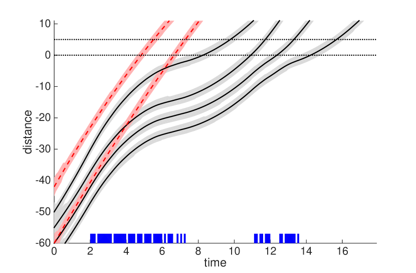
Refer to caption
(a)
Refer to caption
(b)
Figure 6: Simulation of the exact supervisor s𝑠s in (a) and the efficient supervisor sesubscript𝑠𝑒s_{e} in (b). The dotted lines at distance 0 and 5 represent the location of the intersection. The solid black lines and the dotted red lines are the exact trajectories of the controlled and uncontrolled vehicles, respectively, and the shading around the lines represent the position estimation. The blue boxes on the bottom are the time steps at which the supervisor overrides the controlled vehicles. The initial exact state is 𝐲(0)=𝐲0absent\mathbf{y}(0)=(-42, -50, -55, -60, -60, -65) and 𝐯(0)=𝐯0absent\mathbf{v}(0)=(10, 9, 8, 8, 10, 8).

In summary, the efficient supervisors s^^𝑠\hat{s} and sesubscript𝑠𝑒s_{e} are more restrictive than the exact supervisor s𝑠s, and s^^𝑠\hat{s} is more restrictive than sesubscript𝑠𝑒s_{e} by Theorem 5.

6 Simulations

In this section, we present simulation results of the exact and efficient supervisors, s𝑠s and sesubscript𝑠𝑒s_{e}, in two scenarios by running Algorithms 2 and 6. These are implemented using MATLAB on a personal computer with an 3.10 GHz Intel Core i7-3770s processor with 8 GB RAM.

With the dynamic states xj=(yj,vj)subscript𝑥𝑗subscript𝑦𝑗subscript𝑣𝑗x_{j}=(y_{j},v_{j}) and xγ=(yγ,vγ)subscript𝑥𝛾subscript𝑦𝛾subscript𝑣𝛾x_{\gamma}=(y_{\gamma},v_{\gamma}) for j𝒞𝑗𝒞j\in\mathcal{C} and γ𝒞¯𝛾¯𝒞\gamma\in\bar{\mathcal{C}}, the vehicle dynamics considered in the simulation are as follows:

y˙j=vj+dy,j,subscript˙𝑦𝑗subscript𝑣𝑗subscript𝑑𝑦𝑗\displaystyle\dot{y}_{j}=v_{j}+d_{y,j},
v˙j={max(0,ujbvj2+dv,j)if(vj=vj,min),min(0,ujbvj2+dv,j)if(vj=vj,max),ujbvj2+dv,jotherwise,subscript˙𝑣𝑗cases0subscript𝑢𝑗𝑏superscriptsubscript𝑣𝑗2subscript𝑑𝑣𝑗ifsubscript𝑣𝑗subscript𝑣𝑗𝑚𝑖𝑛0subscript𝑢𝑗𝑏superscriptsubscript𝑣𝑗2subscript𝑑𝑣𝑗ifsubscript𝑣𝑗subscript𝑣𝑗𝑚𝑎𝑥subscript𝑢𝑗𝑏superscriptsubscript𝑣𝑗2subscript𝑑𝑣𝑗otherwise\displaystyle\dot{v}_{j}=\begin{cases}\max(0,u_{j}-bv_{j}^{2}+d_{v,j})&\text{if}~{}(v_{j}=v_{j,min}),\\ \min(0,u_{j}-bv_{j}^{2}+d_{v,j})&\text{if}~{}(v_{j}=v_{j,max}),\\ u_{j}-bv_{j}^{2}+d_{v,j}&\text{otherwise},\end{cases}

and

y˙γ=vγ+dy,γ,subscript˙𝑦𝛾subscript𝑣𝛾subscript𝑑𝑦𝛾\displaystyle\dot{y}_{\gamma}=v_{\gamma}+d_{y,\gamma},
v˙γ={max(0,wγbvγ2+dv,γ)if(vγ=vγ,min),min(0,wγbvγ2+dv,γ)if(vγ=vγ,max),wγbvγ2+dv,γotherwise,subscript˙𝑣𝛾cases0subscript𝑤𝛾𝑏superscriptsubscript𝑣𝛾2subscript𝑑𝑣𝛾ifsubscript𝑣𝛾subscript𝑣𝛾𝑚𝑖𝑛0subscript𝑤𝛾𝑏superscriptsubscript𝑣𝛾2subscript𝑑𝑣𝛾ifsubscript𝑣𝛾subscript𝑣𝛾𝑚𝑎𝑥subscript𝑤𝛾𝑏superscriptsubscript𝑣𝛾2subscript𝑑𝑣𝛾otherwise\displaystyle\dot{v}_{\gamma}=\begin{cases}\max(0,w_{\gamma}-bv_{\gamma}^{2}+d_{v,\gamma})&\text{if}~{}(v_{\gamma}=v_{\gamma,min}),\\ \min(0,w_{\gamma}-bv_{\gamma}^{2}+d_{v,\gamma})&\text{if}~{}(v_{\gamma}=v_{\gamma,max}),\\ w_{\gamma}-bv_{\gamma}^{2}+d_{v,\gamma}&\text{otherwise},\end{cases}

where b=0.001𝑏0.001b=0.001 is a drag coefficient, and dy,j,dy,γ,dv,i,dv,γsubscript𝑑𝑦𝑗subscript𝑑𝑦𝛾subscript𝑑𝑣𝑖subscript𝑑𝑣𝛾d_{y,j},d_{y,\gamma},d_{v,i},d_{v,\gamma} are disturbances representing unmodeled dynamics bounded by 0.050.05-0.05 and 0.050.050.05. The speeds vj,vγsubscript𝑣𝑗subscript𝑣𝛾v_{j},v_{\gamma} are bounded by vj,min=vγ,min=1.39subscript𝑣𝑗𝑚𝑖𝑛subscript𝑣𝛾𝑚𝑖𝑛1.39v_{j,min}=v_{\gamma,min}=1.39 and vj,max=vγ,max=13.9subscript𝑣𝑗𝑚𝑎𝑥subscript𝑣𝛾𝑚𝑎𝑥13.9v_{j,max}=v_{\gamma,max}=13.9, the input ujsubscript𝑢𝑗u_{j} by uj,min=2.5subscript𝑢𝑗𝑚𝑖𝑛2.5u_{j,min}=-2.5 and uj,max=2.5subscript𝑢𝑗𝑚𝑎𝑥2.5u_{j,max}=2.5, and the driver-input wγsubscript𝑤𝛾w_{\gamma} by wγ,min=0.5subscript𝑤𝛾𝑚𝑖𝑛0.5w_{\gamma,min}=-0.5 and wγ,max=0.5subscript𝑤𝛾𝑚𝑎𝑥0.5w_{\gamma,max}=0.5. In the simulation, the disturbances and the driver-inputs of uncontrolled vehicles are randomly chosen within their bounds.

At each time step τ=0.1𝜏0.1\tau=0.1, the supervisors determine whether there are impending collisions at an intersection located at (αi,βi)=(0,5)subscript𝛼𝑖subscript𝛽𝑖05(\alpha_{i},\beta_{i})=(0,5) for all i𝒞𝒞¯𝑖𝒞¯𝒞i\in\mathcal{C}\cup\bar{\mathcal{C}}. The states of all vehicles are measured subject to noises, δy,i[3,3]subscript𝛿𝑦𝑖33\delta_{y,i}\in[-3,3] and δv,i[0.05,0.05]subscript𝛿𝑣𝑖0.050.05\delta_{v,i}\in[-0.05,0.05]. For the sake of simplicity, in the simulation, we let uj,desirek=1superscriptsubscript𝑢𝑗𝑑𝑒𝑠𝑖𝑟𝑒𝑘1u_{j,desire}^{k}=1 for all vehicles at all times.

In the first scenario, four controlled and two uncontrolled vehicles are approaching an intersection as in Figure 6, which illustrates the position trajectories of the vehicles in time.

The simulation result of the exact supervisor s𝑠s is shown in Figure 6(a), and that of the efficient supervisor sesubscript𝑠𝑒s_{e} is shown in Figure 6(b). Though we said in Section 5.2 that sesubscript𝑠𝑒s_{e} is more conservative than s𝑠s – in the sense that given the same initial condition, s𝑠s evaluates more inputs to find one guaranteeing avoiding the Bad set than sesubscript𝑠𝑒s_{e} – comparison of the override time steps (blue boxes) in Figures 6(a) and 6(b) indicates that sesubscript𝑠𝑒s_{e} does not override the drivers more than s𝑠s. It takes 0.067 s and 0.011 s per iteration to execute s𝑠s (Algorithm 2) and sesubscript𝑠𝑒s_{e} (Algorithm 6), respectively, in the worst case. This validates that the computation of the efficient supervisor is faster than that of the exact supervisor. In both simulations, the intersection at distance (0,5)05(0,5) is occupied by one vehicle at a time.

Refer to caption
Figure 7: Simulation of the efficient supervisor sesubscript𝑠𝑒s_{e}. The initial exact state is 𝐲(0)=𝐲0absent\mathbf{y}(0)=(-25, -30, -35, -40, -45, -50, -55, -60, -65, -65, -70, -75, -80, -85) and 𝐯(0)=𝐯0absent\mathbf{v}(0)=(6,9, 9, 8, 8, 8, 8, 8, 8, 9.5, 8, 8, 8, 8).

The second scenario considers twelve controlled and two uncontrolled vehicles. Due to the large number of controlled vehicles involved, the exact supervisor cannot solve the verification problem within one time step. Thus, the only option to resolve conflict in this scenario is to implement the efficient supervisor (Algorithm 6). As shown in Figure 7, the efficient supervisor assists the vehicles to prevent any collision at the intersection. In the worst case, it takes 0.033 s per iteration.

7 Experiments

In this section, we describe the experimental validation of the exact supervisor on an intersection testbed. First, we introduce the laboratory apparatus. Then, we describe the dynamic model of the RC cars used in the experiment and the techniques adopted to reduce disturbances. The results of the experiment are provided at the end of this section.

7.1 Experimental setup
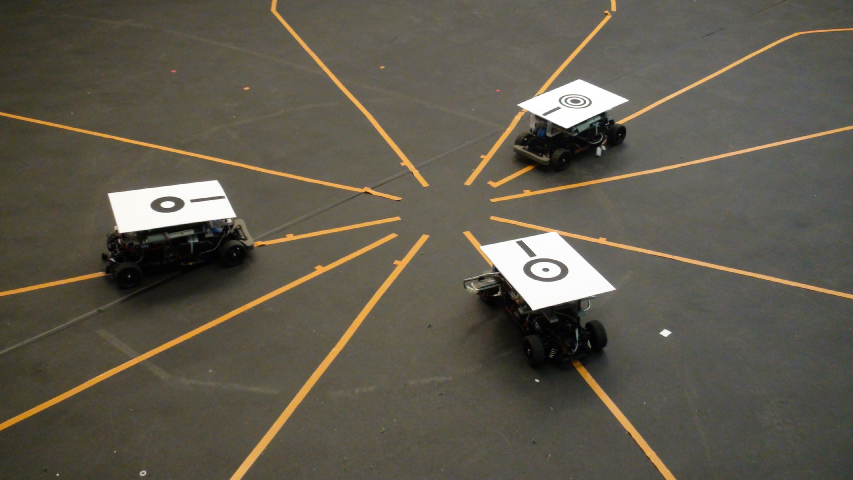
Refer to caption
(a)
Refer to caption
(b)
Figure 8: (a) The RC cars used in the experiment. The camera system detects their symbols to identify each car and measure its position. (b) The paths of the cars on the testbed. Cars 1 and 2 are controlled by the supervisor while car 3 is not. A car is considered to be occupying the intersection when its position is within the shaded circle.

The cars used for this experiment are each built onto a Tamiya scaled RC car chassis equipped with a DC motor. A micro-controller (Acroname Moto 1.0) is used to control the steering servo and the motor through two separate PWM channels. An on-board computer (Mini-ITX running Fedora) runs the C programs, which provide the functionalities required to communicate with the centralized supervisor and to control the micro-controller. The system is powered by two batteries (Tenergy Li-Ion 14.8 V 4400 mAh) connected to a capacitor (Aluminium Electrolytic Capacitor 12000 uF 25 V) through a power relay (Omron G5SB). A power amplifier (Acroname 3 A Back EMF H-bridge) connected to the batteries through a switch provides necessary power to the motor.

During the experiment, three cars follow distinct paths intersecting at a single point on a 6 m ×\times 6 m testbed as shown in Figure 8(b). Each path is stored as sequential points on the coordinate system illustrated in the figure. Cars 1 and 2 are controlled by the exact supervisor when necessary, while car 3 is not controllable. We program cars 1 and 2 to maintain constant motor input, which corresponds to the desired input, while car 3 is driven by a human operator.

Each car has access to its own wheel speed through a quadrature encoder mounted on the rear axle. The position and direction of the cars are measured by an over-head vision system, which comprises six cameras on the ceiling and three computers processing images taken by the cameras. Each car is identified by a symbol attached to its roof as shown in Figure 8(a). The measurement of the speeds, positions, and directions of all cars are collected by an external computer via a wireless connection of the 802.11b standard using UDP/IP. Then, the computer distributes these measurements to the controlled cars, together with other information such as the desired inputs of the controlled vehicles and model parameters discussed in the next section.

7.2 Car dynamics model

Refer to caption
Figure 9: Block diagram of the RC car model. The model includes the measurement disturbances δy,isubscript𝛿𝑦𝑖\delta_{y,i} and δv,isubscript𝛿𝑣𝑖\delta_{v,i} on the car position and speed, respectively.

A block diagram in Figure 9 represents the car dynamics. In this section, we design a compensating input to reduce the effects of the disturbances dproj,i,dpower,i,dslope,isubscript𝑑𝑝𝑟𝑜𝑗𝑖subscript𝑑𝑝𝑜𝑤𝑒𝑟𝑖subscript𝑑𝑠𝑙𝑜𝑝𝑒𝑖d_{proj,i},d_{power,i},d_{slope,i}, and dsteer,isubscript𝑑𝑠𝑡𝑒𝑒𝑟𝑖d_{steer,i}.

Before compensating for the disturbances, the dynamics of the RC cars are as follows: for car i𝒞𝒞¯𝑖𝒞¯𝒞i\in\mathcal{C}\cup\bar{\mathcal{C}} where 𝒞={1,2}𝒞12\mathcal{C}=\{1,2\} and 𝒞¯={3}¯𝒞3\bar{\mathcal{C}}=\{3\},

y˙i=vi+dproj,i,v˙i=aivi+bi+fiui+dpower,i+dslope,i+dsteer,iformulae-sequencesubscript˙𝑦𝑖subscript𝑣𝑖subscript𝑑𝑝𝑟𝑜𝑗𝑖subscript˙𝑣𝑖subscript𝑎𝑖subscript𝑣𝑖subscript𝑏𝑖subscript𝑓𝑖subscript𝑢𝑖subscript𝑑𝑝𝑜𝑤𝑒𝑟𝑖subscript𝑑𝑠𝑙𝑜𝑝𝑒𝑖subscript𝑑𝑠𝑡𝑒𝑒𝑟𝑖\displaystyle\begin{split}&\dot{y}_{i}=v_{i}+d_{proj,i},\\ &\dot{v}_{i}=a_{i}v_{i}+b_{i}+f_{i}u_{i}+d_{power,i}+d_{slope,i}+d_{steer,i}\end{split} (29)

where yisubscript𝑦𝑖{y}_{i} is the longitudinal position of car i𝑖i along the path, visubscript𝑣𝑖v_{i} is its wheel speed, and uisubscript𝑢𝑖u_{i} is the motor input with model parameters ai,bi,subscript𝑎𝑖subscript𝑏𝑖a_{i},b_{i}, and fisubscript𝑓𝑖f_{i}. The disturbances dproj,i,dpower,i,dslope,isubscript𝑑𝑝𝑟𝑜𝑗𝑖subscript𝑑𝑝𝑜𝑤𝑒𝑟𝑖subscript𝑑𝑠𝑙𝑜𝑝𝑒𝑖d_{proj,i},d_{power,i},d_{slope,i}, and dsteer,isubscript𝑑𝑠𝑡𝑒𝑒𝑟𝑖d_{steer,i} are explained below and compensated to reduce their effects.
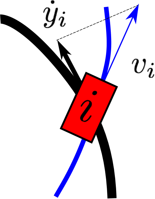
Refer to caption
(a)
Refer to caption
(b)
Figure 10: Cases when dproj,i0subscript𝑑𝑝𝑟𝑜𝑗𝑖0d_{proj,i}\neq 0. Imperfect path following contributes to the discrepancy between the longitudinal speed y˙isubscript˙𝑦𝑖\dot{y}_{i} and the wheel speed visubscript𝑣𝑖v_{i}.

Notice that visubscript𝑣𝑖v_{i} is the car’s wheel speed while yi˙˙subscript𝑦𝑖\dot{y_{i}} is the projected speed on the longitudinal path of car i𝑖i. It is possible that yi˙vi˙subscript𝑦𝑖subscript𝑣𝑖\dot{y_{i}}\neq v_{i} when the car does not follow its path exactly, and this discrepancy is represented by the term dproj,isubscript𝑑𝑝𝑟𝑜𝑗𝑖d_{proj,i}. Figure 10 shows two cases in which y˙ivisubscript˙𝑦𝑖subscript𝑣𝑖\dot{y}_{i}\neq v_{i}. In Figure 10(a), the direction of car i𝑖i differs from the tangent of the longitudinal path (black line) so that viy˙isubscript𝑣𝑖subscript˙𝑦𝑖v_{i}\neq\dot{y}_{i}. In Figure 10(b), two cars follow the same path with the same wheel speed v𝑣v but with slight deviation from the path, causing y˙i>v>y˙jsubscript˙𝑦𝑖𝑣subscript˙𝑦𝑗\dot{y}_{i}>v>\dot{y}_{j}.

Refer to caption
(a)
Refer to caption
(b)
Figure 11: The results of implementing the exact supervisor (see also Extension 1). The intersection is represented by the dotted lines located at (0,65)065(0,65) cm. The solid black lines represent the position measurement of the controlled cars, cars 1 and 2, and the dotted red line represents the position measurement of the uncontrolled car, car 3. These figures demonstrate that the cars are not inside the intersection at the same time.

This dynamic model (LABEL:eq:rccarmodel) includes three different disturbances on the acceleration. The disturbance dpower,isubscript𝑑𝑝𝑜𝑤𝑒𝑟𝑖d_{power,i} describes the first-order dynamic behavior empirically observed in the motor as a consequence of the power connection. By running the cars in a circle with constant motor input for several minutes, we can model dpower,i=giet/hiuisubscript𝑑𝑝𝑜𝑤𝑒𝑟𝑖subscript𝑔𝑖superscript𝑒𝑡subscript𝑖subscriptsuperscript𝑢𝑖d_{power,i}=g_{i}e^{-t/h_{i}}u^{\prime}_{i}, where gisubscript𝑔𝑖g_{i} is the gain and hisubscript𝑖h_{i} the time constant. The car-specific parameters gisubscript𝑔𝑖g_{i} and hisubscript𝑖h_{i} are estimated by analyzing the collected data using the least square method (see Rizzi (2014) for the data).

The disturbance dslope,isubscript𝑑𝑠𝑙𝑜𝑝𝑒𝑖d_{slope,i} is introduced to model the slope of the testbed, which is not completely flat and has non-negligible effects on the car speed. The disturbance dsteer,isubscript𝑑𝑠𝑡𝑒𝑒𝑟𝑖d_{steer,i} takes into account the fact that the steering and motor dynamics are coupled (Verma et al. (2008)). Since the testbed slope and the steering input are approximately the same at the same point of the path, we estimate these two disturbances as a path-dependent function dpath,i(y):=dsteer,i(y)+dslope,i(y)assignsubscript𝑑𝑝𝑎𝑡𝑖𝑦subscript𝑑𝑠𝑡𝑒𝑒𝑟𝑖𝑦subscript𝑑𝑠𝑙𝑜𝑝𝑒𝑖𝑦d_{path,i}(y):=d_{steer,i}(y)+d_{slope,i}(y). This function is different for each path and estimated by running the car multiple times and curve fitting of the obtained data.

Eliminating the effects of these disturbances is critical because otherwise it is difficult to initiate Algorithm 2 with a feasible initial condition, especially in a spatially constrained environment, such as a laboratory testbed. To this end, we introduce a compensating term ci(t,yi)subscript𝑐𝑖𝑡subscript𝑦𝑖c_{i}(t,y_{i}) to the motor input so that ui=ui+ci(t,yi)subscript𝑢𝑖subscriptsuperscript𝑢𝑖subscript𝑐𝑖𝑡subscript𝑦𝑖u_{i}=u^{\prime}_{i}+c_{i}(t,y_{i}), where uisuperscriptsubscript𝑢𝑖u_{i}^{\prime} is the input signal returned by the supervisor for car i𝑖i. By employing the model and estimation of the disturbances explained above, we obtain the following compensating input:

ci(t,yi)=giet/hiui+dpath,i(yi)giet/hi+fi.subscript𝑐𝑖𝑡subscript𝑦𝑖subscript𝑔𝑖superscript𝑒𝑡subscript𝑖subscriptsuperscript𝑢𝑖subscript𝑑𝑝𝑎𝑡𝑖subscript𝑦𝑖subscript𝑔𝑖superscript𝑒𝑡subscript𝑖subscript𝑓𝑖c_{i}(t,y_{i})=-\frac{g_{i}e^{-t/h_{i}}u^{\prime}_{i}+d_{path,i}(y_{i})}{g_{i}e^{-t/h_{i}}+f_{i}}.

This, in turn, simplifies (LABEL:eq:rccarmodel) as y˙i=vi+dproj,isubscript˙𝑦𝑖subscript𝑣𝑖subscript𝑑𝑝𝑟𝑜𝑗𝑖\dot{y}_{i}=v_{i}+d_{proj,i} and v˙i=aivi+bi+fiuisubscript˙𝑣𝑖subscript𝑎𝑖subscript𝑣𝑖subscript𝑏𝑖subscript𝑓𝑖subscriptsuperscript𝑢𝑖\dot{v}_{i}=a_{i}v_{i}+b_{i}+f_{i}u^{\prime}_{i}. Eventually with the compensation, we consider the following car dynamics in the experiment. For i𝒞𝒞¯𝑖𝒞¯𝒞i\in\mathcal{C}\cup\bar{\mathcal{C}},

y˙i=vi+dy,i,subscript˙𝑦𝑖subscript𝑣𝑖subscript𝑑𝑦𝑖\displaystyle\dot{y}_{i}=v_{i}+d_{y,i},
v˙i={max(0,aivi+bi+fiui+dv,i)if(vi=vi,min),min(0,aivi+bi+fiui+dv,i)if(vi=vi,max),aivi+bi+fiui+dv,iotherwise,subscript˙𝑣𝑖cases0subscript𝑎𝑖subscript𝑣𝑖subscript𝑏𝑖subscript𝑓𝑖superscriptsubscript𝑢𝑖subscript𝑑𝑣𝑖ifsubscript𝑣𝑖subscript𝑣𝑖𝑚𝑖𝑛0subscript𝑎𝑖subscript𝑣𝑖subscript𝑏𝑖subscript𝑓𝑖superscriptsubscript𝑢𝑖subscript𝑑𝑣𝑖ifsubscript𝑣𝑖subscript𝑣𝑖𝑚𝑎𝑥subscript𝑎𝑖subscript𝑣𝑖subscript𝑏𝑖subscript𝑓𝑖subscriptsuperscript𝑢𝑖subscript𝑑𝑣𝑖otherwise\displaystyle\dot{v}_{i}=\begin{cases}\max(0,a_{i}v_{i}+b_{i}+f_{i}u_{i}^{\prime}+d_{v,i})&\text{if}~{}(v_{i}=v_{i,min}),\\ \min(0,a_{i}v_{i}+b_{i}+f_{i}u_{i}^{\prime}+d_{v,i})&\text{if}~{}(v_{i}=v_{i,max}),\\ a_{i}v_{i}+b_{i}+f_{i}u^{\prime}_{i}+d_{v,i}&\text{otherwise},\end{cases}

where dv,isubscript𝑑𝑣𝑖d_{v,i} represents an error from the compensation and an unpredicted source of disturbance.

7.3 Results
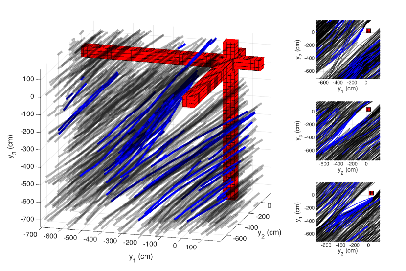
Refer to caption
Figure 12: Trajectories (semitransparent black lines) in the output space. There are 509 trajectories, which are indicated in blue when the supervisor intervenes. The three figures on the right-hand side are the 2D projections. These confirm that all of the trajectories avoid the Bad set.

The on-board computers on cars 1 and 2 run Algorithm 2. Since the same algorithm is run with the same measurement updated every τ=0.1s𝜏0.1𝑠\tau=0.1s, the outputs are the same, thereby working as centralized control.

The parameters are as follows: a=𝑎absenta=(-0.53, -0.30, -0.43) s-1, b=𝑏absentb=(-84.68, -66.43, -49.64) cm/s2, g=𝑔absentg=(0.99, 0.44, 0.95), and h=absenth=(9.17, 6.84, 5.95) s. The gain fi(t)subscript𝑓𝑖𝑡f_{i}(t) for all i𝑖i is a time-varying parameter, estimated at every time step. The bounds of the speed are vmin=subscript𝑣𝑚𝑖𝑛absentv_{min}=(10.5, 10.5, 13) cm/s and vmax=subscript𝑣𝑚𝑎𝑥absentv_{max}=(17, 16.5, 15) cm/s, and those of the motor input (PWM) are umin=(105,105,130)subscript𝑢𝑚𝑖𝑛105105130u_{min}=(105,105,130) and umax=subscript𝑢𝑚𝑎𝑥absentu_{max}=(170,165,150). The bounds of the measurement noises are empirically chosen by ignoring long tails as δy,i,min=subscript𝛿𝑦𝑖𝑚𝑖𝑛absent\delta_{y,i,min}= -25 cm, δy,i,max=subscript𝛿𝑦𝑖𝑚𝑎𝑥absent\delta_{y,i,max}= 25 cm, δv,i,min=subscript𝛿𝑣𝑖𝑚𝑖𝑛absent\delta_{v,i,min}= -25 cm/s, and δv,i,max=subscript𝛿𝑣𝑖𝑚𝑎𝑥absent\delta_{v,i,max}= 16 cm/s for all i𝑖i. The bounds of the experimental disturbance are dy,min=subscript𝑑𝑦𝑚𝑖𝑛absentd_{y,min}=(-5, -3, -3) cm/s, dy,max=subscript𝑑𝑦𝑚𝑎𝑥absentd_{y,max}=(3, 4, 3) cm/s, dv,min=subscript𝑑𝑣𝑚𝑖𝑛absentd_{v,min}=(-4, -2, -3) cm/s2, and dv,max=subscript𝑑𝑣𝑚𝑎𝑥absentd_{v,max}=(2, 3, 2.5) cm/s2.

Figure 11 depicts two experimental results obtained by implementing the exact supervisor. The intersection is located at (0, 65) cm for all cars. The intersection is an area containing the point at which the paths intersect, as in Figure 8(b).

In Figure 11(a), in picture 1, the uncontrolled car (dotted red circle) approaches the intersection earlier than the other cars. The supervisor overrides the controlled cars (solid blue circles) to decelerate them until their desired inputs do not cause conflict. In picture 2, the conflict is resolved, and one controlled car crosses the intersection alone without overrides. In Figure 11(b), in picture 1, one controlled car approaches the intersection first. The supervisor lets this car accelerate and the other controlled car decelerate so that the uncontrolled car safely crosses the intersection, as shown in picture 2. Notice that the upper bound of the last car’s position enters the intersection right after the lower bound of the uncontrolled car’s position has exited, indicating that the override was applied because it is deemed necessary to avoid the collision. In both cases, intersection collisions are averted.

Figure 12 depicts 509 trajectories (semitransparent black lines) near the Bad set (red blocks). The trajectories are indicated in blue when the supervisor intervenes. From the 2D projections (figures on the right-hand side), we can confirm that none of the trajectories enters the Bad set. Since cars 1 and 2 are programmed to maintain constant speeds and car 3 does not change its speed quickly, the trajectories in the projections should be straight lines without overrides. We can see that the supervisor overrides cars 1 and 2 when the trajectories would enter the Bad set if the trajectories were linear. We observed in 15 trajectories that the cars were forced to stop before the Bad set because the supervisor could not find a safe input. This was because we had to truncate the tails of the distributions of disturbances, and thus the state measurement and the state estimation can sometimes be incompatible. This truncation is necessary in the confined laboratory because otherwise a feasible initial condition may not always exist. The existence of a feasible initial condition is a necessary condition to initiate procedure Supervisor in Algorithm 2.

8 Conclusions

We have designed exact and efficient supervisors that override controlled vehicles when collisions are imminent. The sources of uncertainty, such as measurement errors, unmodeled dynamics, and the presence of uncontrolled vehicles are taken into account in the design of the supervisors. The exact supervisor determines the existence of safe inputs (verification problem) by solving the Inserted Idle-Time (IIT) scheduling problem, which is proven to yield equivalent answers to the verification problem. To address the computational complexity issue, we also design the efficient supervisor that solves the IIT scheduling problem with a quantified approximation bound. The simulation results show that the efficient supervisor prevents collisions without substantial conservatism, compared to the exact one. The experiment using RC cars on an intersection testbed validated that collisions at an intersection are successfully averted by the exact supervisor.

Although this paper deals only with decision problems to focus on safety, there is no barrier to incorporate objective functions to address other issues such as fuel consumption or traffic congestion. The intersection considered in this paper is modeled as a single conflict area so that vehicles are required to occupy the intersection one at a time. This assumption may make the system very conservative in that, for example, two vehicles turning right on different lanes are geometrically unable to collide while the supervisors do not let them inside the intersection at the same time. We are currently investigating the design of supervisors with a more general intersection model, which includes multi-conflict points. The result with simple first-order vehicle dynamics can be found in Ahn and Del Vecchio (2016, To appear). Other remaining issues include preventing rear-end collisions (Colombo and Del Vecchio (2014)) and considering unknown routes of vehicles.

{funding}

This work was in part supported by NSF Award #1239182. Alessandro Colombo was in part supported by grant AD14VARI02 - Sottomisura B.

References

  • Ahn et al. (2014) Ahn H, Colombo A and Del Vecchio D (2014) Supervisory control for intersection collision avoidance in the presence of uncontrolled vehicles. In: American Control Conference (ACC). pp. 867–873.
  • Ahn and Del Vecchio (2016, To appear) Ahn H and Del Vecchio D (2016, To appear) Semi-autonomous intersection collision avoidance through job-shop scheduling. In: the 19th ACM international conference on Hybrid Systems: Computation and Control.
  • Ahn et al. (2015) Ahn H, Rizzi A, Colombo A and Del Vecchio D (2015) Experimental testing of a semi-autonomous multi-vehicle collision avoidance algorithm at an intersection testbed. In: IEEE/RSJ International Conference on Intelligent Robots and Systems (IROS). pp. 4834–4839.
  • Alonso-Ayuso et al. (2011) Alonso-Ayuso A, Escudero L and Martín-Campo F (2011) Collision Avoidance in Air Traffic Management: A Mixed-Integer Linear Optimization Approach. IEEE Transactions on Intelligent Transportation Systems 12(1): 47–57.
  • Borrelli et al. (2006) Borrelli F, Subramanian D, Raghunathan A and Biegler L (2006) MILP and NLP Techniques for centralized trajectory planning of multiple unmanned air vehicles. In: American Control Conference.
  • Bruni et al. (2013) Bruni L, Colombo A and Del Vecchio D (2013) Robust multi-agent collision avoidance through scheduling. In: IEEE Conference on Decision and Control (CDC). pp. 3944–3950.
  • Cassandras and Lafortune (2008) Cassandras CG and Lafortune S (eds.) (2008) Introduction to Discrete Event Systems. Boston, MA: Springer US.
  • Colombo and Del Vecchio (2012) Colombo A and Del Vecchio D (2012) Efficient algorithms for collision avoidance at intersections. In: the 15th ACM international conference on Hybrid Systems: Computation and Control. pp. 145––154.
  • Colombo and Del Vecchio (2014) Colombo A and Del Vecchio D (2014) Least Restrictive Supervisors for Intersection Collision Avoidance: A Scheduling Approach. IEEE Transactions on Automatic Control 10.1109/TAC.2014.2381453.
  • Cormen et al. (2009) Cormen TH, Leiserson CE, Rivest RL and Stein C (2009) Introduction to Algorithms. 3rd edition edition. Cambridge: The MIT Press. ISBN 9780262033848.
  • Garey et al. (1981) Garey MR, Johnson DS, Simons BB and Tarjan RE (1981) Scheduling Unit–Time tasks with arbitrary release times and deadlines. SIAM Journal on Computing 10: 256–269.
  • Gillula et al. (2011) Gillula JH, Hoffmann GM, Huang H, Vitus MP and Tomlin CJ (2011) Applications of hybrid reachability analysis to robotic aerial vehicles. The International Journal of Robotics Research 30(3): 335–354.
  • Hafner et al. (2013) Hafner M, Cunningham D, Caminiti L and Del Vecchio D (2013) Cooperative Collision Avoidance at Intersections: Algorithms and Experiments. IEEE Transactions on Intelligent Transportation Systems 14(3): 1162–1175.
  • Hafner and Del Vecchio (2011) Hafner MR and Del Vecchio D (2011) Computational tools for the safety control of a class of piecewise continuous systems with imperfect information on a partial order. SIAM Journal on Control and Optimization 49: 2463–2493.
  • Hoffmann and Tomlin (2008) Hoffmann G and Tomlin C (2008) Decentralized cooperative collision avoidance for acceleration constrained vehicles. In: IEEE Conference on Decision and Control (CDC). pp. 4357–4363.
  • Kamal et al. (2014) Kamal M, Imura J, Hayakawa T, Ohata A and Aihara K (2014) A Vehicle-Intersection Coordination Scheme for Smooth Flows of Traffic Without Using Traffic Lights. IEEE Transactions on Intelligent Transportation Systems 10.1109/TITS.2014.2354380.
  • Kowshik et al. (2011) Kowshik H, Caveney D and Kumar P (2011) Provable systemwide safety in intelligent intersections. IEEE Transactions on Vehicular Technology 60: 804–818.
  • Lee and Park (2012) Lee J and Park B (2012) Development and evaluation of a cooperative vehicle intersection control algorithm under the connected vehicles environment. IEEE Transactions on Intelligent Transportation Systems 13: 81–90.
  • Maimone et al. (2007) Maimone M, Cheng Y and Matthies L (2007) Two years of Visual Odometry on the Mars Exploration Rovers. Journal of Field Robotics 24(3): 169–186. 10.1002/rob.20184.
  • Mastellone et al. (2008) Mastellone S, Stipanović DM, Graunke CR, Intlekofer KA and Spong MW (2008) Formation Control and Collision Avoidance for Multi-agent Non-holonomic Systems: Theory and Experiments. The International Journal of Robotics Research 27(1): 107–126.
  • Pallottino et al. (2002) Pallottino L, Feron E and Bicchi A (2002) Conflict resolution problems for air traffic management systems solved with mixed integer programming. IEEE Transactions on Intelligent Transportation Systems 3(1): 3–11.
  • Peng and Akella (2005a) Peng J and Akella S (2005a) Coordinating Multiple Double Integrator Robots on a Roadmap: Convexity and Global Optimality. In: IEEE International Conference on Robotics and Automation (ICRA). pp. 2751–2758.
  • Peng and Akella (2005b) Peng J and Akella S (2005b) Coordinating Multiple Robots with Kinodynamic Constraints Along Specified Paths. The International Journal of Robotics Research 24(4): 295–310.
  • Richards et al. (2002) Richards A, Schouwenaars T, How JP and Feron E (2002) Spacecraft Trajectory Planning with Avoidance Constraints Using Mixed-Integer Linear Programming. Journal of Guidance, Control, and Dynamics 25(4): 755–764.
  • Rizzi (2014) Rizzi A (2014) Analysis and optimization of an experimental apparatus to test active safety systems in vehicles. URL https://www.politesi.polimi.it/handle/10589/92232.
  • Smith et al. (2010) Smith RN, Chao Y, Li PP, Caron DA, Jones BH and Sukhatme GS (2010) Planning and Implementing Trajectories for Autonomous Underwater Vehicles to Track Evolving Ocean Processes Based on Predictions from a Regional Ocean Model. The International Journal of Robotics Research 29(12): 1475–1497.
  • Verma et al. (2008) Verma R, Del Vecchio D and Fathy H (2008) Development of a Scaled Vehicle With Longitudinal Dynamics of an HMMWV for an ITS Testbed. IEEE/ASME Transactions on Mechatronics 13(1): 46–57. 10.1109/TMECH.2008.915820.
  • Wu et al. (2012) Wu J, Abbas-Turki A and El Moudni A (2012) Cooperative driving: an ant colony system for autonomous intersection management. Applied Intelligence 37: 207–222.
  • Wurman et al. (2008) Wurman PR, D’Andrea R and Mountz M (2008) Coordinating Hundreds of Cooperative, Autonomous Vehicles in Warehouses. AI Magazine 29(1): 9–19.

Appendix A: Index to Multimedia Extensions

Extension Media type Description
1 Video This video contains experiments of the exact supervisor presented in Section 7.

Appendix B

We provide the proofs of Lemmas 1-3 in this section.

Lemma 1. Procedure Polynomial in Algorithm 3 solves the IIT scheduling problem with unit process times and finds a feasible schedule if exists.

Proof.

To account for inserted idle-times, we define an initial set of forbidden regions as F0,γ=(r¯γ1,p¯γ)subscript𝐹0𝛾subscript¯𝑟𝛾1subscript¯𝑝𝛾F_{0,\gamma}=(\bar{r}_{\gamma}-1,\bar{p}_{\gamma}) for all γ𝛾\gamma. If tjF0,γsubscript𝑡𝑗subscript𝐹0𝛾t_{j}\notin F_{0,\gamma} for some j𝑗j, then we have (tj,tj+1)(r¯γ,p¯γ)=subscript𝑡𝑗subscript𝑡𝑗1subscript¯𝑟𝛾subscript¯𝑝𝛾(t_{j},t_{j}+1)\cap(\bar{r}_{\gamma},\bar{p}_{\gamma})=\emptyset, thereby satisfying condition (21).

Forbidden Region Declaration in lines 3-11 of procedure Polynomial solves Problem 4. The key idea is critical time c𝑐c, which is the latest start time of job σisubscript𝜎𝑖\sigma_{i}. If job σisubscript𝜎𝑖\sigma_{i} starts later than critical time c𝑐c, at least one of the subsequent jobs cannot be scheduled before its deadline. That is, if a job cannot start before the critical time (line 10), there is no schedule satisfying conditions (19)-(21). Otherwise, there will be a schedule satisfying all the conditions. This relation between critical time and the existence of a feasible schedule was proved in Garey et al. (1981) with initially empty forbidden regions. Since initially non-empty forbidden regions do not affect the fact that critical time is the latest start time, this analysis of critical time can determine the existence of a schedule with non-empty initial forbidden regions.

With the forbidden regions declared, the EDD rule finds a schedule in lines 12-17. Time s𝑠s is assigned to each job as a schedule. In line 14, s𝑠s avoids the forbidden regions so that condition (21) is satisfied. If there is no ready job (line 15), a job with the minimum release time among unscheduled jobs is scheduled, and otherwise (line 16), a job with the earliest deadline among ready jobs is scheduled. After a job is scheduled, line 17 updates s𝑠s to s+1𝑠1s+1 so that condition (20) is satisfied. This schedule cannot satisfy condition (19) if ans𝑎𝑛𝑠ans has been no𝑛𝑜no in line 10. Otherwise, this schedule satisfies conditions (19)-(21).∎∎

Lemma 2. If Approx([𝐱a(0),𝐱b(0)],S)=(𝐓,yes)superscript𝐱𝑎0superscript𝐱𝑏0𝑆𝐓𝑦𝑒𝑠([\mathbf{x}^{a}(0),\mathbf{x}^{b}(0)],S)=(\mathbf{T},yes), and RelaxedExact([𝐱a(0),𝐱b(0)],S)=(𝐓¯,π,yes)superscript𝐱𝑎0superscript𝐱𝑏0𝑆¯𝐓superscript𝜋𝑦𝑒𝑠([\mathbf{x}^{a}(0),\mathbf{x}^{b}(0)],S)=(\bar{\mathbf{T}},\pi^{*},yes), then TjT¯jsubscript𝑇𝑗subscript¯𝑇𝑗T_{j}\leq\bar{T}_{j} for all j𝒞𝑗𝒞j\in\mathcal{C}.

Proof.

We will show by induction on j𝑗j that TπjT¯πjsubscript𝑇subscriptsuperscript𝜋𝑗subscript¯𝑇subscriptsuperscript𝜋𝑗T_{\pi^{*}_{j}}\leq\bar{T}_{\pi^{*}_{j}} for all πjsubscriptsuperscript𝜋𝑗\pi^{*}_{j}\in\mathcal{M}. Notice that Ti=T¯i=0subscript𝑇𝑖subscript¯𝑇𝑖0T_{i}=\bar{T}_{i}=0 for all i¯𝑖¯i\in\bar{\mathcal{M}}. The schedule 𝐓𝐓\mathbf{T} is generated by procedure Scheduling in Algorithm 1. For the base case, Tπ1=max(Rπ1,Pmax)subscript𝑇subscriptsuperscript𝜋1subscript𝑅subscriptsuperscript𝜋1subscript𝑃𝑚𝑎𝑥T_{\pi^{*}_{1}}=\max(R_{\pi^{*}_{1}},P_{max}) in line 8 of Algorithm 1. Since T¯π1subscript¯𝑇subscriptsuperscript𝜋1\bar{T}_{\pi^{*}_{1}} is a feasible solution of Problem 5 by Lemma 1, it satisfies Rπ1T¯π1subscript𝑅subscriptsuperscript𝜋1subscript¯𝑇subscriptsuperscript𝜋1R_{\pi^{*}_{1}}\leq\bar{T}_{\pi^{*}_{1}} from condition (23) and (0,Pi(0))(T¯π1,T¯π1+θmax)=0subscript𝑃𝑖0subscript¯𝑇subscriptsuperscript𝜋1subscript¯𝑇subscriptsuperscript𝜋1subscript𝜃𝑚𝑎𝑥(0,P_{i}(0))\cap(\bar{T}_{\pi^{*}_{1}},\bar{T}_{\pi^{*}_{1}}+\theta_{max})=\emptyset for all i¯𝑖¯i\in\bar{\mathcal{M}} from condition (24). Thus, max(Rπ1,Pmax)=Tπ1T¯π1subscript𝑅subscriptsuperscript𝜋1subscript𝑃𝑚𝑎𝑥subscript𝑇subscriptsuperscript𝜋1subscript¯𝑇subscriptsuperscript𝜋1\max(R_{\pi^{*}_{1}},P_{max})=T_{\pi^{*}_{1}}\leq\bar{T}_{\pi^{*}_{1}}. Now, suppose Tπk1T¯πk1subscript𝑇subscriptsuperscript𝜋𝑘1subscript¯𝑇subscriptsuperscript𝜋𝑘1T_{\pi^{*}_{k-1}}\leq\bar{T}_{\pi^{*}_{k-1}}. Then, for j=k𝑗𝑘j=k, we need to show that TπkT¯πksubscript𝑇subscriptsuperscript𝜋𝑘subscript¯𝑇subscriptsuperscript𝜋𝑘T_{\pi^{*}_{k}}\leq\bar{T}_{\pi^{*}_{k}}.

In line 10 of Algorithm 1, Tπk=max(Rπk,Tπk1+Pπk1(Tπk1))subscript𝑇subscriptsuperscript𝜋𝑘subscript𝑅subscriptsuperscript𝜋𝑘subscript𝑇subscriptsuperscript𝜋𝑘1subscript𝑃subscriptsuperscript𝜋𝑘1subscript𝑇subscriptsuperscript𝜋𝑘1T_{\pi^{*}_{k}}=\max(R_{\pi^{*}_{k}},T_{\pi^{*}_{k-1}}+P_{\pi^{*}_{k-1}}(T_{\pi^{*}_{k-1}})). If Tπk=Rπksubscript𝑇subscriptsuperscript𝜋𝑘subscript𝑅subscriptsuperscript𝜋𝑘T_{\pi^{*}_{k}}=R_{\pi^{*}_{k}}, we have TπkT¯πksubscript𝑇subscriptsuperscript𝜋𝑘subscript¯𝑇subscriptsuperscript𝜋𝑘T_{\pi^{*}_{k}}\leq\bar{T}_{\pi^{*}_{k}} because T¯πksubscript¯𝑇subscriptsuperscript𝜋𝑘\bar{T}_{\pi^{*}_{k}} satisfies condition (23). If Tπk=Tπk1+Pπk1(Tπk1)subscript𝑇subscriptsuperscript𝜋𝑘subscript𝑇subscriptsuperscript𝜋𝑘1subscript𝑃subscriptsuperscript𝜋𝑘1subscript𝑇subscriptsuperscript𝜋𝑘1T_{\pi^{*}_{k}}=T_{\pi^{*}_{k-1}}+P_{\pi^{*}_{k-1}}(T_{\pi^{*}_{k-1}}), we have TπkT¯πk1+θmaxsubscript𝑇subscriptsuperscript𝜋𝑘subscript¯𝑇subscriptsuperscript𝜋𝑘1subscript𝜃𝑚𝑎𝑥T_{\pi^{*}_{k}}\leq\bar{T}_{\pi^{*}_{k-1}}+\theta_{max} because Tπk1T¯πk1subscript𝑇subscriptsuperscript𝜋𝑘1subscript¯𝑇subscriptsuperscript𝜋𝑘1T_{\pi^{*}_{k-1}}\leq\bar{T}_{\pi^{*}_{k-1}} and Pπk1(Tπk1)θmaxsubscript𝑃subscriptsuperscript𝜋𝑘1subscript𝑇subscriptsuperscript𝜋𝑘1subscript𝜃𝑚𝑎𝑥P_{\pi^{*}_{k-1}}(T_{\pi^{*}_{k-1}})\leq\theta_{max} by (22). Since T¯πksubscript¯𝑇subscriptsuperscript𝜋𝑘\bar{T}_{\pi^{*}_{k}} satisfies condition (24), T¯πk1+θmaxT¯πksubscript¯𝑇subscriptsuperscript𝜋𝑘1subscript𝜃𝑚𝑎𝑥subscript¯𝑇subscriptsuperscript𝜋𝑘\bar{T}_{\pi^{*}_{k-1}}+\theta_{max}\leq\bar{T}_{\pi^{*}_{k}}. Therefore, TπkT¯πksubscript𝑇subscriptsuperscript𝜋𝑘subscript¯𝑇subscriptsuperscript𝜋𝑘T_{\pi^{*}_{k}}\leq\bar{T}_{\pi^{*}_{k}}. In lines 13 and 15 of Algorithm 1, the schedule can increase so that Tπk=P¯γsubscript𝑇subscriptsuperscript𝜋𝑘subscript¯𝑃𝛾T_{\pi^{*}_{k}}=\bar{P}_{\gamma} for some γ𝒞¯𝛾¯𝒞\gamma\in\bar{\mathcal{C}} if TπkR¯γsubscript𝑇subscriptsuperscript𝜋𝑘subscript¯𝑅𝛾T_{\pi^{*}_{k}}\geq\bar{R}_{\gamma} or Tπk+Pπk(Tπk)>R¯γsubscript𝑇subscriptsuperscript𝜋𝑘subscript𝑃subscriptsuperscript𝜋𝑘subscript𝑇subscriptsuperscript𝜋𝑘subscript¯𝑅𝛾T_{\pi^{*}_{k}}+P_{\pi^{*}_{k}}(T_{\pi^{*}_{k}})>\bar{R}_{\gamma}. Since T¯πksubscript¯𝑇subscriptsuperscript𝜋𝑘\bar{T}_{\pi^{*}_{k}} satisfies condition (25), if T¯πkR¯γsubscript¯𝑇subscriptsuperscript𝜋𝑘subscript¯𝑅𝛾\bar{T}_{\pi^{*}_{k}}\geq\bar{R}_{\gamma} or T¯πk+θmax>R¯γsubscript¯𝑇subscriptsuperscript𝜋𝑘subscript𝜃𝑚𝑎𝑥subscript¯𝑅𝛾\bar{T}_{\pi^{*}_{k}}+\theta_{max}>\bar{R}_{\gamma}, then it must be T¯πkP¯γsubscript¯𝑇subscriptsuperscript𝜋𝑘subscript¯𝑃𝛾\bar{T}_{\pi^{*}_{k}}\geq\bar{P}_{\gamma}. Therefore, in either case, TπkT¯πksubscript𝑇subscriptsuperscript𝜋𝑘subscript¯𝑇subscriptsuperscript𝜋𝑘T_{\pi^{*}_{k}}\leq\bar{T}_{\pi^{*}_{k}}. ∎∎

Lemma 3. If Approx([𝐱a(0),𝐱b(0)],S)=(,no)superscript𝐱𝑎0superscript𝐱𝑏0𝑆𝑛𝑜([\mathbf{x}^{a}(0),\mathbf{x}^{b}(0)],S)=(\emptyset,no), then RelaxedExact([𝐱a(0),𝐱b(0)],S)=(,π,no)superscript𝐱𝑎0superscript𝐱𝑏0𝑆superscript𝜋𝑛𝑜([\mathbf{x}^{a}(0),\mathbf{x}^{b}(0)],S)=(\emptyset,\pi^{*},no).

Proof.

In Algorithm 5, procedure Approx returns no if [𝐲a(0),𝐲b(0)]Bsuperscript𝐲𝑎0superscript𝐲𝑏0𝐵[\mathbf{y}^{a}(0),\mathbf{y}^{b}(0)]\cap B\neq\emptyset in line 2 or procedure Scheduling with πsuperscript𝜋\pi^{*} returns no𝑛𝑜no in line 5. In the former case, procedure RelaxedExact also returns no as in line 2 of Algorithm 4. The latter case implies that Tπj>Dπjsubscript𝑇subscriptsuperscript𝜋𝑗subscript𝐷subscriptsuperscript𝜋𝑗T_{\pi^{*}_{j}}>D_{\pi^{*}_{j}} for some πj𝒞subscriptsuperscript𝜋𝑗𝒞\pi^{*}_{j}\in\mathcal{C}. By Lemma 2, we have T¯πjTπjsubscript¯𝑇subscriptsuperscript𝜋𝑗subscript𝑇subscriptsuperscript𝜋𝑗\bar{T}_{\pi^{*}_{j}}\geq T_{\pi^{*}_{j}} if a feasible solution 𝐓¯¯𝐓\bar{\mathbf{T}} of Problem 5 exists. Such a schedule cannot be feasible because T¯πjTπj>Dπjsubscript¯𝑇subscriptsuperscript𝜋𝑗subscript𝑇subscriptsuperscript𝜋𝑗subscript𝐷subscriptsuperscript𝜋𝑗\bar{T}_{\pi^{*}_{j}}\geq T_{\pi^{*}_{j}}>D_{\pi^{*}_{j}}, which does not satisfy condition (23). Thus, procedure RelaxedExact returns (,π,no)superscript𝜋𝑛𝑜(\emptyset,\pi^{*},no). ∎∎