The Cosmological Lithium Problem Revisited

Abstract

After a brief review of the cosmological lithium problem, we report a few recent attempts to find theoretical solutions by our group at Texas A&M University (Commerce & College Station). We will discuss our studies on the theoretical description of electron screening, the possible existence of parallel universes of dark matter, and the use of non-extensive statistics during the Big Bang nucleosynthesis epoch. Last but not least, we discuss possible solutions within nuclear physics realm. The impact of recent measurements of relevant nuclear reaction cross sections for the Big Bang nucleosynthesis based on indirect methods is also assessed. Although our attempts may not able to explain the observed discrepancies between theory and observations, they suggest theoretical developments that can be useful also for stellar nucleosynthesis.

1 INTRODUCTION

The so-called lithium problem is one of the most resilient puzzles in nuclear astrophysics. It is quickly becoming as well known as the solar neutrino problem which ruled for many years as a seed for the development of theoretical physics imagination [1, 2, 3, 4]. It eventually was solved with an old idea: that neutrinos can oscillate [5]. The solar neutrino problem is arguably one of the main reasons for the strong investment on neutrino astrophysics during the last decades, which ultimately led to two neutrino physics related nobel prizes a few years back. It was a sad decision by the Nobel committee that John Bahcall was not awarded with this prize as he was the most creative physicist in neutrino astrophysics before and after the very first design of the Homestake experiment [6]. Among several possibilities to solve the puzzle was thought to be in nuclear physics, e.g., the ⁷Be(p,$\gamma$)⁸B reaction, responsible for the high energy neutrinos coming from the core of the sun [7, 8]. But only a drastic modification of the low energy astrophysical S-factor for this and other reactions would solve the solar neutrino puzzle. The solution came indeed from the unusual character of the neutrino as a fundamental particle, which took a long time to be proven experimentally.

In contrast to the solar neutrino problem, there are no hints that the cosmological lithium problem can be solved without closely assessing the role of nuclear reactions, during the Big Bang, or in stellar environments. A few minutes ($\sim 4-20$ m) after the Big Bang, nuclei started forming first with the creation of the deuteron by neutron capture on proton, p(n,$\gamma$)d. The formation of deuterons is strongly dependent on the baryon-to-photon ratio in the Big Bang epoch, $\eta_{b}=\#baryons/\#photons$. After the deuteron bottleneck is surpassed, all other heavier elements are synthesized, and are also therefore strongly dependent on $\eta_{b}$. Other important parameters of Big Bang nucleosynthesis are the neutron lifetime and the number of neutrino species. Because deuterons are promptly consumed once they are formed, a significant amount of ³He is created by means of the (p,$\gamma)^{3}$He and d(d,n)³He reactions. Tritium is also synthesized by means of d(d,p)t reaction. The creation of ⁴He nuclei then follows by the ³He(d,p)⁴He and t(d,n)⁴He reactions. After hydrogen (75%), helium (25%) is the most abundant element in the visible universe. The correct prediction of the hydrogen and helium abundance is one of the major successes of the Big Bang model. It is necessary to have a neutron-to-proton ratio, n/p = 1/7, when the Big Bang nucleosynthesis started in order to explain the observed values of hydrogen and helium abundance. Thus, Big Bang nucleosynthesis occurred in a proton-rich environment.

A series of reactions involving neutron, proton, deuteron, and helium captures allow elements up to lithium and beryllium to be created during the Big Bang. ${}^{7}{\rm Li}$ and ${}^{6}{\rm Li}$, were synthesized in very small amounts, with the ⁷Li/H abundance of the order of $10^{-10}$ and ⁶Li/H of the order of $10^{-14}$. Not only the deuteron, but also the ⁷Li abundance is strongly dependent on the value of $\eta_{b}$. Big Bang nucleosynthesis is not the only source of lithium isotopes. ⁶Li can also be produced in cosmic rays due to spallation reactions and ⁷Li can be formed in novae and pulsations of AGB stars. Spite and Spite [9, 10] have noticed that the ⁷Li abundance was nearly independent of the metallicity in metal-poor stars. Metal poor stars are defined as those with a small Fe/H abundance relative to the sun. The logarithm of this ratio is denoted by [Fe/H]. In low metallicity stars $-2.4\leq[{\rm Fe/H}]\leq-1.4$. The observations were done for warm ($5700\leq T\leq 6250$ K) metal-poor dwarf stars. The nearly constant ⁷Li abundance, nearly independent of metallicity and temperature, is known as the Spite plateau. White dwarfs at moderate temperatures have been used in such studies because warmer stars, such as red giants, reaching temperatures in excess of $10^{6}$ K lead to the destruction of ⁷Li via the reaction ${}^{7}{\rm Li}({\rm p},\alpha){}^{4}{\rm He}$. Based on the Spite plateau observations, a reasonable conclusion is that lithium is not created or depleted in warm dwarfs, even over a rather large variation of temperature. It is thus natural to conclude that the Spite plateau consists in a firm observation of the primordial ⁷Li abundance, synthesized during the Big Bang epoch. But it is important to notice that there have been recent observations in low-metallicity stars which seem to be at odds with the Spite plateau [11, 12].

Big Bang nucleosynthesis leads to robust predictions which have survived the test of observations. Observations of lithium abundance in metal poor halo stars [12] yield ${}^{7}{\rm Li/H}=1.58^{+0.35}_{-0.28}\times 10^{-10}$ which is appreciably smaller than the value of ${}^{7}{\rm Li/H}=4.46\times 10^{-10}$ predicted by Big Bang Nucleosynthesis (BBN) [13]. This difference has survived a large number of tests and is the source of the lithium puzzle. An additional problem is the abundance of ${}^{6}{\rm Li}$ created in the BBN by means of the ${}^{2}{\rm H}(\alpha,\gamma)^{6}{\rm Li}$ reaction. When ${}^{6}{\rm Li}$ is formed within stars, it disappears quickly by means of other nuclear reactions. One believes that it is mainly created by cosmic rays, but one also believes that it can exist in the atmosphere of halo metal-poor warm dwarfs, surviving destruction by cosmic rays. But this assumption is controversial, as the same hypotheses can be applied to ${}^{7}{\rm Li}$ nuclei. While the BBN predicts a primordial isotopic ratio ${}^{6}{\rm Li}/{}^{7}{\rm Li}\sim 10^{-5}$ [13], some observations report a value ${}^{6}{\rm Li}/{}^{7}{\rm Li}\sim 5\times 10^{-2}$ [14]. This discrepancy is an addition to the BBN lithium puzzle and is known as the second lithium problem. Such findings have been disputed and the complexity of 3D models for convection and non-local thermodynamical equilibrium in the photo-sphere of metal-poor stars can lead to a substantial weakening of the second lithium problem, leading to isotopic ratios in better agreement with the BBN predictions [15].

2 ENVIRONMENT ELECTRONS

It is well known that nuclear reaction cross sections at the low energies of interest for astrophysics are enhanced because of the presence of electrons in the environment. Electrons bound in the atoms as well as free electrons, as those present in stellar plasmas, reduce the Coulomb repulsion between nuclei and enhance the chances for tunneling through the Coulomb barrier. There have been experimental evidences that the effect of atomic electrons is not well described by theory [16]. In laboratory experiments, the cross section enhancement due to bound electrons in targets is larger than predicted by apparently all existing models in theory [17]. In stars, or during the Big Bang, the cross section enhancement due to free electrons is quantified by the enhancement factor $f(E)={\sigma_{s}(E)/\sigma_{b}(E)}$, where $\sigma_{s}$ is the screened cross section and $\sigma_{b}$ is the bare cross section, without influence of electrons. This factor is usually calculated using the Debye-Hückel approximation, yielding a screened Coulomb potential in the weak screening limit (for $\langle V\rangle\ll kT$), so that $V(r)=({e^{2}Z_{i}/r})\exp\left(-{r/R_{D}}\right)$. This leads to an enhancement factor [16]

$$f=\;\mathrm{exp}\left({Z_{1}\,Z_{2}\;e^{2}\over R_{D}kT}\right)=\;\mathrm{exp}\left({0.188\,Z_{1}\,Z_{2}\;\zeta\;\rho^{1/2}\;T_{6}^{-3/2}}\right),$$ (1)

where the Debye radius is given by

$$R_{D}={1\over\zeta}\left({kT\over 4\pi e^{2}n}\right)^{1/2},$$ (2)

with the number density given by $n$, the density $\rho$ given in units of g/cm³, and

$$\zeta=\left[\sum\limits_{i}~{}X_{i}~{}\frac{Z_{i}^{2}}{A_{i}}+\chi\sum\limits_{i}~{}X_{i}\frac{Z_{i}}{A_{i}}\right]^{1/2}.$$ (3)

In this equation, the mass fraction of particle $i$ is given by $X_{i}$, the temperature $T_{6}$ is given in units of 10⁶ K, and $\chi$ is a factor correcting for electron degeneracy effects [18].

There have been some discussions in the literature about the magnitude of screening effects and deviations form the Debye-Hückel model [19, 20, 21, 22]. Applications of this approximation to the plasma in the core of the sun yields 3-5 of particles within the Debye-Hückel. This does not validate the use of mean-field approximations inherent to the derivation of the Eq. (1). A better method to describe the screening in such cases is the use of molecular dynamics simulations [19, 20] but these do not seem to reproduce the mean field models. Electron screening is also dependent on the electron velocities in the plasma [23]. Some lingering questions remain on the use of the Salpeter formula, Eq. (1), used to explain the experiments on electron screening [24, 25]. Other theoretical methods have also defied the traditional dependence on the Debye-Hückel approximation to describe electron screening in stars [26, 27]. Based on this discussion and the theoretical difficulty to reproduce the experimental data on laboratory screening of the astrophysical nuclear cross section and explain the stellar plasma screening at content, it is not far-fetched to assume that there might be strong deviations of the Debye-Hückel approximation. In Ref. [28] this possibility was explored in order to verify if electron screening could modify appreciably the abundance of elements formed in the BBN (see also, Ref. [29]).

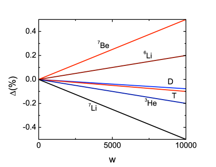
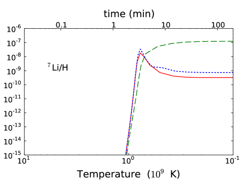
Figure 1: Left: Percent change in the abundances of light nuclei synthesized during the BBN as a function the fudge factor $w$ modifying the Debye-Hückel screening formula (Adopted from Ref. [28]). Right: ⁷Li abundance in the BBN using reaction rates calculated with Maxwell distributions (solid curves) and with non-extensive statistics with $q=0.5$ (dotted line) and $q=2$ (dashed line) (Adopted from Ref. [34]).

In the early universe, the electron density decreased strongly as the temperature decreased and it was much larger (by up to $10^{4}$ times) than the density in the core of the sun ($n_{e}^{sun}\sim 10^{26}$/cm³). The baryonic density depends on the temperature as $\rho_{b}\simeq hT_{9}^{3}$ ($T_{9}$ is the temperature in units of $10^{9}$ K), with $h$ being the baryon density parameter [30]. $h$ changes value around $T_{9}\sim 2$ from $h\sim 2.1\times 10^{-5}$ to $h\sim 5.7\times 10^{-5}$. During the BBN the electron density was much larger than in the sun, but the baryon density was much smaller. The number of excess electrons is nearly the same as those of protons, with most of the remaining ones being equal to the number of positrons produced via $\gamma\gamma\rightarrow e^{+}e^{-}$ processes. From these considerations, one can calculate the enhancement factor in Eq. (1) and show that it becomes independent of the temperature [28],

$$f^{BBN}=\exp\left(4.49\times 10^{-8}\zeta Z_{1}Z_{2}\right)\sim 1+4.49\times 10^{-8}\zeta Z_{1}Z_{2}\ \ \ {\rm for}\ \ T_{9}\lesssim 1,$$ (4)

and

$$f^{BBN}=\exp\left(2.71\times 10^{-8}\zeta Z_{1}Z_{2}\right)\sim 1+2.71\times 10^{-8}\zeta Z_{1}Z_{2}\ \ \ {\rm for}\ \ T_{9}\gtrsim 2.$$ (5)

In both situations the screening effect is vey small, unless one appreciably modifies the Deby-Hückel approximation.

In Ref. [28] the Debye-Hückel approximation was modified by including an artificial factor $w$, so that

$$f^{\prime}=\;\mathrm{exp}\left(w{Z_{1}\,Z_{2}\;e^{2}\over R_{D}kT}\right),\ \ \ \ \ {\rm or}\ \ \ \ln f^{\prime}=w\ln f,$$ (6)

where $1\leq w\leq 10^{4}$. The modified BBN abundances, $Y^{\prime}$ were calculated using a standard BBN model [28] and the relative change $\Delta={(Y^{\prime}-Y)/Y}$ is shown in Figure 1. It is seen that as $w$ increases, the BBN abundances for ⁶Li and ⁷Be increase, but the abundances for D, T, ³He and ⁷Li decrease. But even if $w$ is as large as $10^{4}$ the modification of the BBN abundances is minimal. Thus, one concludes that the electron screening does not change BBN abundances appreciably and much less it can be identified as a solution of the lithium problem.

3 NON-EXTENSIVE STATISTICS

For the calculation of reaction rates in the BBN one assumes the validity of the Maxwell-Boltzmann (MB) distribution of velocities of the nuclei in a plasma. The MB distribution is based on the Boltzmann-Gibbs statistics, which assumes that (a) the average time between collisions is much larger than the collision time, (b) the interaction occurs locally, (c) there is no correlation between the velocities of two particles in a given location in space, and (d) the energy is conserved without transfer of energy from collective degrees of freedom. These are strongly constraining assumptions which do not always hold for systems in thermodynamical equilibrium. Variations of the Boltzmann-Gibbs (BG) statistics have been proposed in Refs. [31, 32, 33]. In Ref. [34], the departure from the extensive BG statistics has been studied in the context of the BBN. The motivation was again to check if this would have any visible effect on the lithium abundances and a possible relation to the lithium puzzle. We adopted the non-extensive statistics proposed by Tsallis [32, 33], which encompasses a large family of entropies, each depending on a parameter $q$, which serves as a measure of the departure from the extensive BG statistics. When $q=1$ the BG statistics is recovered from the Tsallis statistics.

The standard BBN model has been very successful and one cannot expect that a large departure from the BG statistics is possible. That is, the non-extensive parameter $q$ cannot be much different than $q=1$. In Ref. [34], the value of $q$ was varied substantially so that the departure from the BBN predicted abundances can become visible. The deviation from the Maxwellian velocity distribution and its consequences for nuclear burning in stars has also been investigated in Refs. [35, 36, 37, 38]. The entropy in the BG statistics is given by ${\cal S}_{BG}=-k_{B}\sum_{i}p_{i}\ln p_{i}$, where $p_{i}$ is the probability to find the system in the i-th microstate. If $A$ and $B$ are two independent systems, the probability of $A+B$ to be found in a state $i+j$, is $p^{A+B}_{i+j}=p^{A}_{i}\cdot p^{B}_{j}$. This yields the extensive property of the BG entropy, ${\cal S}_{A+B}={\cal S}_{A}+{\cal S}_{B}$. In this case, a non-Maxwellian velocity distribution will be valid for particles in a plasma. For a Maxwellian distribution, the reaction rate in stellar plasmas is assumed to be

$$r_{ij}=\frac{N_{i}N_{j}}{1+\delta_{ij}}\langle\sigma v\rangle=\frac{N_{i}N_{j}}{1+\delta_{ij}}\left(\frac{8}{\pi\mu}\right)^{\frac{1}{2}}\left(\frac{1}{k_{B}T}\right)^{\frac{3}{2}}\int_{0}^{\infty}dES(E)\exp\left[-\left(\frac{E}{k_{B}T}+2\pi\eta(E)\right)\right],$$ (7)

with $\sigma$ being the cross section, $v$ the relative velocity of the particles $i$, $j$, $N_{i}$ the number of particles $i$, $\mu$ the reduced mass, $T$ the temperature, and $S(E)$ the astrophysical S-factor. $\eta=Z_{i}Z_{j}e^{2}/\hbar v$ is the Sommerfeld parameter, for charges $Z_{i}$ and $Z_{j}$ and the relative energy of $i+j$ is given by $E=\mu v^{2}/2$. The astrophysical S-factor is defined as $S(E)=E\sigma(E)\exp\left[{2\pi\eta(E)}\right]$. For neutron induced reactions it is more appropriate to use the definition $\sigma(E)={R(E)/\sqrt{E}}$ because the neutron-nucleus cross sections at low energies typically behave as $\sigma\propto 1/v$.

The effects of a non-extensive statistics for BBN has been used to make predictions for the abundances of ⁴He, D, ³He, and ⁷Li and for the reaction rates of p(n,$\gamma$)d, d(p,$\gamma){{}^{3}}$He, d(d,n)³He, d(d,p)t, ³He(n,p)t, t(d,n)⁴He, ³He(d,p)⁴He, ³He$(\alpha,\gamma){{}^{7}}$Be, t$(\alpha,\gamma){{}^{7}}$Li, ⁷Be(n,p)⁷Li and ⁷Li(p,$\alpha){{}^{4}}$He using the available experimental data of these reactions [34]. As an example, Figure 1 (right) shows the ⁷Li abundance, where the solid curve uses Maxwell distributions to calculate reaction rates while non-extensive distributions have been used for $q=0.5$ (dotted line) and for $q=2$ (dashed line). We see that in both cases, the ⁷Li abundance increases. This also occurs for values either below or slightly above $q=1$. In Table 1, we show the BBN predictions for element abundance using Maxwellian and non-Maxwellian distributions. All figures have the same power of ten as in the observational data presented in the last column.

Table 1: BBN predictions for element abundance using Maxwellian and non-Maxwellian distributions. All figures have the same power of ten as in the observational data [40] presented in the last column [34].

	Maxwell	Non-Max.	Non-Max.	Observation
	BBN	$q=0.5$	$q=2$
4He/H	0.249	0.243	0.141	$0.2561\pm 0.0108$
D/H	2.62	3.31	570	$2.82^{+0.20}_{-0.19}$($\times 10^{-5}$)
3He/H	0.98	0.91	69.1	$(1.1\pm 0.2)$($\times 10^{-5}$)
7Li/H	4.39	6.89	356.	$(1.58\pm 0.31)(\times 10^{-10})$

We conclude that it is not possible to solve the lithium puzzle with use of a non-extensive statistics to calculate the reaction rates during the BBN. The departure from the BG statistics in fact worsens the lithium problem by increasing its abundance. The details for the reasons of this increase are explained in Ref. [34]. As seen in Table 1, the abundances of the other elements are also substantially affected by a departure from the extensive statistics. A chi-square fit to the observations has revealed a very narrow window for the non-extensive parameter of the order of $q=1.00^{+0.05}_{-0.02}$ [34].

4 NUCLEAR CROSS SECTIONS UNCERTAINTIES

The experimental values of the nuclear reaction cross sections of interest for nuclear astrophysics can be fitted using the R-matrix method, where the resonances and background are obtained by solving the Schrödinger equation with matching conditions at a channel radius, or radii. The method leads to the reproduction of phase shifts and cross sections described in terms of a small set of parameters, and by extrapolation one obtains the cross sections at the low astrophysical energies. The matching condition at the channel radii leads to S-matrix poles at energies $E_{\lambda}$, and reduced widths, $\gamma_{\lambda}$. The energy dependence of the R-matrix becomes

$$R_{ij}(E)=\sum_{\lambda=1}^{N}{\gamma_{\lambda i}\gamma_{\lambda j}\over E_{\lambda}-E},$$ (8)

where $i$ and $j$ denote the reaction channels, with momentum, $J$, and parity, $\Pi$. The reduced widths, $\gamma_{\lambda i}$ are related to solutions of the Schrödinger equation for each channel radius [41]. In Ref. [13] R-matrix fits have been done to a collection of data based on direct and indirect measurements such as those obtained recently with the Trojan Horse Method (THM). Various nuclear reaction rates are among the most important input parameters for the BBN nucleosynthesis, but only the main 12 reactions listed in Table 2 have been considered [42].

${\rm n}\leftrightarrow{\rm p}$	${\rm p(n,}\gamma{\rm)d}$	${\rm d(p,}\gamma)^{3}{\rm He}$	${\rm d(d,p)t}$
${\rm d(d,n)}^{3}{\rm He}$	${}^{3}{\rm He(n,p)t}$	${\rm t(d,n)}^{4}{\rm He}$	${}^{3}{\rm He(d,p)}^{4}{\rm He}$
${}^{3}{\rm He}(\alpha,\gamma)^{7}{\rm Be}$	${\rm t(}\alpha,\gamma)^{7}{\rm Li}$	${}^{7}{\rm Be(n,p)}^{7}{\rm Li}$	${}^{7}{\rm Li(p,}\alpha)^{4}{\rm He}$

Table 2: The 12 most relevant nuclear reactions during the BBN.

In Figure 2 we show the calculated BBN abundance of ³He, ⁴He, D and ⁷Li as a function of time and temperature using best fits to existing experimental data [13]. The black curve is for the ⁴He mass fraction, the green curve is the deuterium abundance, the red curve is for the ³He abundance and blue curve for the ⁷Li abundance. Errors in the experimental data are manifest in the error bands around the abundance curves. In Table 3 the BBN calculations using fits to recent experimental data for BBN reactions are compared with observations. Data for (a) are mass fraction for ⁴He from Ref. [43], (b) deuterium abundance from the mean average $\left<({\rm D/H})\right>=(2.82\pm 0.26)\times 10^{-5}$, compatible with $\Omega_{b}h^{2}\ ({\rm BBN})=0.0213\pm 0.0013$ [44], (c) ³He abundances from Ref. [45], (d) lithium abundance from Ref. [12]. It is clear from Figure 2 and Table 3 that the observed lithium depletion puzzle is not so evident when experimental errors in the measured S-factors, or cross sections, are included.

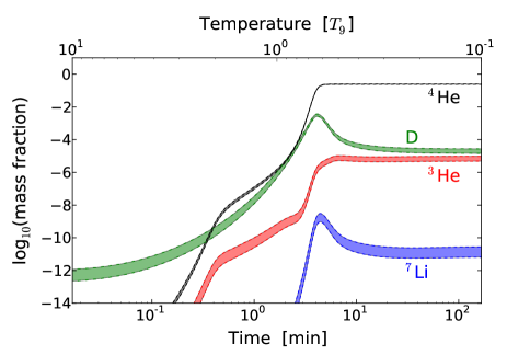
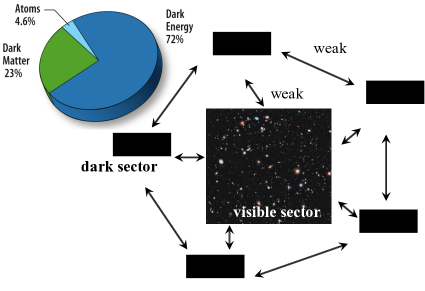
Figure 2: Left: Calculated BBN abundances of ³He, ⁴He, D and ⁷Li as a function of time and temperature using best fits to existing experimental data [13]. The black curve is for the ⁴He mass fraction, the green curve is the deuterium abundance, the red curve is for the ³He abundance and blue curve for the ⁷Li abundance. Errors in the experimental data are manifest in the error bands around the abundance curves. (Adopted from Ref. [13]). Right: Visible matter accounts for only 5% of the energy content in the Universe, while dark matter accounts for about 25% of it.

More recently the second lithium problem, i.e., the disagreement between observations and BBN predictions for the lithium ⁶Li/⁷Li isotopic ratio was discussed in Ref. [46]. While BBN predictions are ${}^{6}{\rm Li}/^{7}{\rm Li}\sim 10^{-5}$, observations yield ${}^{6}{\rm Li}/^{7}{\rm Li}\sim 2\times 10^{-2}$ [14]. In Ref. [46] a re-analysis of the reaction ⁴He$(\alpha,\gamma)^{6}$Li was performed, including new predictions for angular distribution. A nice agreement with recent experimental data from the LUNA collaboration [47] was found. This result reinforces the BBN predictions for the lithium isotopic ratio and leads to a new value of ${}^{6}{\rm Li}/^{7}{\rm Li}=(1.5\pm 0.3)\times 10^{-5}$ (see also Ref. [15]), which now seems to agree much better with the BBN predictions. We conclude that it is not at all impossible that the problems associated with lithium abundances might not be due to astration of elements, but to accurate measurements combined with better theories for nuclear reactions.

Table 3: BBN calculations using fits to recent experimental data for BBN reactions compared with observations. Data for (a) are mass fraction for ⁴He from Ref. [43], (b) deuterium abundance from the mean average $\left<({\rm D/H})\right>=(2.82\pm 0.26)\times 10^{-5}$, compatible with $\Omega_{b}h^{2}\ ({\rm BBN})=0.0213\pm 0.0013$ [44], (c) ³He abundances from Ref. [45], (d) lithium abundance from Ref. [12].

Yields	Calculation	Observation
$Y_{p}$	0.2485${}^{+0.001}_{-0.002}$	$0.2565\pm 0.006^{(a)}$
D/H ($\times 10^{-5}$)	2.692${}^{+0.177}_{-0.070}$	$2.82\pm 0.26^{(b)}$
3He/H ($\times 10^{-6}$)	9.441${}^{+0.511}_{-0.466}$	$\geq 11.\pm 2.^{(c)}$
7Li/H ($\times 10^{-10}$)	4.683${}^{+0.335}_{-0.292}$	$1.58\pm 0.31^{(d)}$

5 PARALLEL UNIVERSES OF DARK MATTER

Dark Matter (DM) comprises most of the matter in the universe and almost nothing is known about it, except for its gravitational properties [48, 49, 50]. Except for gravity, it interacts very weakly with known baryonic matter, or perhaps not at all. Its existence is based on observations of galaxy clusters dynamics and anisotropies of the Cosmic Microwave Background (CMB). It is possibly composed of hypothetic particles such as Weakly Interacting Massive Particles (WIMPs), supersymmetric particles, sterile neutrinos, etc. DM could be built up of mirror(s) sector(s) of particles [51, 52, 53, 54, 55] with each mirror sector being composed of particle copies of the Standard Model (SM), but not exact copies with different masses and couplings.

In Refs. [56, 57] a mirror model of parallel universes was developed based on a not fully explored SU(3) gauge symmetry for multiple universes. Based on the observation for the density parameters $\Omega_{DM}$ and $\Omega_{b}$, there are about 5 times more dark matter than visible matter, more precisely, $\Omega_{DM}/\Omega_{b}=4.94\pm 0.66$. One can assume that there are 5 dark sectors and one visible sector (see Figure 2, right). The dark sectors are exact replicas of the Standard Model (SM) of elementary particle physics. In Ref. [56] one has introduced a new Weakly Interacting Massive Gauge Boson (WIMG) responsible for the coupling between all sectors, also with ordinary matter. The WIMG has to be a massive boson, leaving properties of the SM and gravity unchanged. It also has to be compatible with BBN results and CMB observations. For energies much lower than the electroweak scale, particles are basically massless and one can group matter fields in terms of their intrinsic electric charges

$$Q_{1}=\left(\begin{array}[]{c}u\\ c\\ t\end{array}\right),\quad Q_{2}=\left(\begin{array}[]{c}d\\ s\\ b\end{array}\right),\quad Q_{3}=\left(\begin{array}[]{c}e\\ \mu\\ \tau\end{array}\right),\quad Q_{4}=\left(\begin{array}[]{c}\nu_{e}\\ \nu_{\mu}\\ \nu_{\tau}\end{array}\right)\,,$$ (9)

where the notation $\mathcal{Q}=\left\{Q_{1},Q_{2},Q_{3},Q_{4}\right\}$ will be used next.

A similar structure wcan be assumed for DM, with each DM sector $\mathcal{Q}_{s}$ having 4 multiplets and its own copy of the SM. Their electroweak sectors bosons will couple only within their own sectors. The WIMG gauge field $M^{a}_{\mu}$ couples to matter fields $Q_{i,s}$, where $s$ denotes the $N_{Q}=6$ sectors and $i$ denotes fermions, as in Eq. (9). The mass, $M^{a}_{\mu}$, of the WIMG is generated by a real scalar field $\phi^{a}$, in an adjoint representation of the $SU(3)_{Q}$ group, with the condition that the WIMG interaction is short ranged. The proposed Lagrangian in this gauge theory is

$$\mathcal{L}=-\frac{1}{4}F^{a}_{\mu\nu}F^{a\,\mu\nu}+\sum^{N_{Q}}_{s=1}\sum^{4}_{i=1}\overline{Q}_{i,s}\,\left\{i\gamma^{\mu}D_{\mu}-m_{s}\right\}\,Q_{i,s}+~{}\frac{1}{2}\left(D^{\mu}\phi^{a}\right)\left(D_{\mu}\phi^{a}\right)-V_{oct}(\phi^{a}\phi^{a})+\mathcal{L}_{GF}+\mathcal{L}_{gh},$$ (10)

where $\mathcal{L}_{GF}$ fixes the gauge in the Lagrangian and $\mathcal{L}_{gh}$ carries the ghost terms, $D_{\mu}=\partial_{\mu}+ig_{M}T^{a}M^{a}_{\mu}$ is the covariant derivative, $T^{a}$ are the generators of $SU(3)_{Q}$ and $V_{oct}$ is the potential energy related to $\phi^{a}$. Note that the second term in Eq. (10) includes a sum over all families of fermions. The Lagrangian $\mathcal{L}$ is a sum of the SM in each sector with $s=1,\cdots,N_{Q}$. Terms describing the quantization of the theory are not shown. The WIMG mass arises from the operator $(g^{2}_{M}/2)\,\phi^{c}(T^{a}T^{b})_{cd}\phi^{d}M^{a}_{\mu}M^{b\,\mu}$, by assuming a non-vanishing boson condensate $\langle\phi^{a}\phi^{b}\rangle$ due to local fluctuations of the scalar field. With the additional assumptions that $\langle\phi^{a}\rangle=0$ and $\langle\phi^{a}\phi^{b}\rangle=v^{2}\delta^{ab}$, and using $\mbox{tr}(T^{a}T^{b})=3\,\delta^{ab}$, one gets for the WIMG mass the value $M^{2}=3\,g^{2}_{M}v^{2}$. The new degrees of freedom will increase the early universe expansion rate [58] with implications for the BBN.

The radiation density during the BBN includes a number of new particles with are constrained by the ⁴He abundance and the baryon-to-photon ratio $\eta_{b}$, so that densities and entropies are given by

$$\rho(T)=\frac{\pi^{2}}{30}\,g_{*}(T)\,T^{4}\quad\mbox{and}\quad s(T)=\frac{2\pi^{2}}{45}\,g_{s}(T)\,T^{3},$$ (11)

where

$$g_{*}(T)=\sum_{B}g_{B}\left(\frac{T_{B}}{T}\right)^{4}+\frac{7}{8}\sum_{F}g_{F}\left(\frac{T_{F}}{T}\right)^{4},\ \ \ \ {\rm and}\ \ \ \ g_{s}(T)=\sum_{B}g_{B}\left(\frac{T_{B}}{T}\right)^{3}+\frac{7}{8}\sum_{F}g_{F}\left(\frac{T_{F}}{T}\right)^{3}.$$ (12)

These are the number of degrees of freedom during the BBN, $g_{B(F)}$ for bosons (fermions), $B(F)$, with temperatures $T_{B(F)}$. $T$ denotes the temperature of the photon thermal bath.

If the dark sectors were decoupled, two temperatures would emerge: $T$ for ordinary matter and $T^{\prime}$ for the dark sectors. The energy $\rho^{\prime}(T^{\prime})$ and entropy $s^{\prime}(T^{\prime})$ densities for the dark sectors are given by Eqs. (11) with the substitutions $g_{*}(T)\rightarrow g^{\prime}_{*}(T^{\prime})$, $g_{s}(T)\rightarrow g^{\prime}_{s}(T^{\prime})$, and $T\rightarrow T^{\prime}$. Separate conservation of entropy in visible and dark sectors yields a time independent parameter $x=(s^{\prime}/s)^{1/3}$. If each dark sector has the same matter content as in the visible sector, $g_{s}(T_{0})=g_{s}^{\prime}(T^{\prime}_{0})$, leading to $x=T^{\prime}/T$. The Friedman equation for a radiation dominated epoch is $H(t)=\sqrt{\left(8\pi/3c^{2}\right)\,G_{N}\,\bar{\rho}}$, with the total energy density $\bar{\rho}=\rho\,+\,N_{DM}\,\rho^{\prime}$, where $N_{DM}=N_{Q}-1$ is the number of dark sectors. Using the relation (11) for the density in the dark sectors, $\rho^{\prime}$, leads to

$$H(t)=1.66\,\sqrt{\bar{g}_{*}(T)}\,\frac{T^{2}}{M_{Pl}},\ \ \ \ \ \ {\rm where}\ \ \ \ \ \bar{g}_{*}(T)=g_{*}(T)\left(1+N_{DM}\,a\,x^{4}\right),$$ (13)

where $M_{Pl}$ is the Planck mass and $a=\left(g^{\prime}_{*}/g_{*}\right)\left(g_{s}/g^{\prime}_{s}\right)^{4/3}\sim 1$, for a not too small $T^{\prime}/T$ [58]. At a BBN temperature of about 1 MeV, the degrees of freedom of photons, electrons, positrons and neutrinos are in quasi-equilibrium and $g_{*}(T=1\ {\rm MeV})=10.75$. Due to the additional dark particles, $g_{*}$ changes to $\bar{g}_{*}=g_{*}\left(1+N_{DM}\,x^{4}\right)$. If one tries to explain the ⁴He, ³He, and D abundances, one gets [56] $T^{\prime}/T<0.78/N^{1/4}_{DM}$. With $N_{DM}=5$, this yields $T^{\prime}/T<0.52$, i.e., dark universes have to be always colder than our universe if the observed element abundances are to be reproduced. Other interesting features of the model is that the baryon-to-photon ratio for the dark sectors comes at as $\eta^{\prime}_{b}\sim 2.1\,N^{3/4}_{DM}\eta_{b}$. Using $N_{DM}=5$ one finds $\eta^{\prime}_{b}\sim 7\eta_{b}$, i.e., BBN runs very differently in the visible and in the dark and cold sectors. The additional degrees of freedom were forced to reproduce the observed abundances in the visible universe. Ref. [56] proved that such a model is compatible with what is observed in the visible universe. But turning the argument around and assuming that the similar conditions in the dark sectors were varied, the model would predict different temperatures, baryon-to-photon ratios, and other changes in the visible universe. The impact of these changes on BBN in our visible universe are entirely open to imagination. The lithium problem might find a solution in this way, but at this point in history we cannot really ascertain what would be the physical properties of the dark sectors and what would they mean if no other probes than gravity and a highly hypothetical WIMG would exist.

6 CONCLUSIONS

In this work we have discussed a few studies by our group at Texas A&M University (Commerce & College Station) on the cosmological lithium problem. The goal is by no means to make a comprehensive review of this research field. For this purpose, there exist much more authoritative reviews in the literature (see, e.g., Refs. [59, 60]).

The lithium puzzle is associated with the BBN prediction of ⁷Li being larger than what is observed. The puzzle recalls an equivalent situation with the solar neutrino problem many decades ago. It might be that there is no puzzle at all. The solution might lie in the way that lithium is processed in stars. The solution might as well be in the realm of nuclear physics. As we have discussed in this text, another lithium problem, i.e., the large difference between BBN predictions and observations for the isotopic ratio ⁶Li/⁷Li, might find its solution in the more precise experiments combined with better nuclear reaction theory [46]. Similar cases such as the electron screening puzzle mentioned earlier have recently found a likely solution also in the realm of nuclear physics. For example, as a nuclear clustering phenomena in light nuclei, instead of a solution in atomic physics. Since ⁷Li is produced mainly via the electron capture process ${}^{7}{\rm Be}+e^{-}\rightarrow^{7}{\rm Li}+\nu_{e}$, the destruction of ⁷Be via several channels could also become a possible solution for the puzzle [62]. The fact is that to the present date there is no solid key for this puzzle that has survived detailed tests in theory and experiment. As in the case of the solar neutrino problem, with Pontecorvo’s proposition of neutrino oscillations [5], the answer for the cosmological lithium problem might already have been found and is waiting out there for a confirmation.

7 ACKNOWLEDGMENTS

C.A.B. Acknowledges support from by the U.S. NSF Grant No. 1415656 and the U.S. DOE Grant No. DE-FG02-08ER41533. A. M. M. acknowledges that this material is based upon work supported by the U.S. Department of Energy, Award Number DE-FG02-93ER40773, by the U.S. Department of Energy, National Nuclear Security Administration, Award Number DE-FG52-09NA29467 and by the US National Science Foundation under Award PHY-1415656. O.O. acknowledges financial support from FCT under contract PTDC/FIS/100968/2008.

References

- [1] J. N. Bahcall and M. Pinsonneault, Rev. Mod. Phys. 64, 885 (1992).
- [2] J. N. Bahcall and H. A. Bethe, Phys. Rev. D 47, 1298 (1993).
- [3] W.C. Haxton, Ann. Rev. Astron. Astrop. 33, 459 (1995).
- [4] J.N. Bahcall et al. Phys. Rev. Lett. 78, 171 (1997).
- [5] B. Pontecorvo, Zh. Eksp. Teor. Fiz. 33, 549 (1957); Sov. Phys. JETP 6, 429 (1957).
- [6] W.C. Haxton, Ann. Rev. Nucl. Part. Sci. 59, 1 (2009).
- [7] C.A. Bertulani, Nucl. Phys. A 587, 318 (1995).
- [8] G. Taubes, “Electronic Battle over Solar Neutrinos”, Science 266, 1157 (1994).
- [9] M. Spite and F. Spite, Nature 297, 483 (1982).
- [10] F. Spite and M. Spite, A&A 115, 357 (1982).
- [11] W. Aoki, et al., ApJ. 698, 1803 (2009).
- [12] L. Sbordone, et al., A&A 522, A26 (2010).
- [13] R.G. Pizzone, et al., Astrophys. J. 786, 112 (2014).
- [14] M. Asplund, D. L. Lambert, P. E. Nissen, F. Primas and V. V. Smith, Ap. J. 644, 229 (2006).
- [15] K. Lind, J. Melendez, M. Asplund, R. Collet and Z. Magic, A&A 554, A96 (2013).
- [16] C.A. Bertulani and A. Gade, Physics Reports 485, 195 (2010).
- [17] A. B. Balantekin, C. A. Bertulani, M. S. Hussein, Nucl. Phys. A 627, 324 (1997).
- [18] E.E. Salpeter, Aust. J. Phys. 7, 373 (1954); E.E. Salpeter and H.M. Van Horn, Ap. J. 155, 183 (1969).
- [19] N.J. Shaviv and G. Shaviv, Ap. J. 468, 433 (1996).
- [20] G. Shaviv and N.J. Shaviv, Ap. J. 529, 1054 (2000).
- [21] D. Mao, K. Mussack, and W. Daeppen, Ap J. 701, 1204 (2009).
- [22] A. Weiss, M. Flaskamp, and V.N. Tsytovich, Astron. Astrophys. 371,1123 (2001).
- [23] D. Kremp, M. Schlanges, and W.-D. Kraeft, Quantum Statistics of Non-ideal Plasmas Springer, Berlin, 2005.
- [24] C. Rolfs and E. Somorjai, Nucl. Inst. Meth. B 99, 297 (1995).
- [25] C. Rolfs, Prog. Part. Nucl. Phys. 46, 23 (2001).
- [26] T. E. Liolios, Eur. Phys. J. Volume A18: S1 (2003).
- [27] Michael Hendrix, “Electron Screening in Stellar Environments”, MSc Thesis, Texas A&M University-Commerce (2015).
- [28] B. Wang, C.A. Bertulani, and A.B. Balantekin, Phys. Rev. C 83, 018801 (2011).
- [29] N. Itoh, A. Nishikawa, S. Nozawa, and Y. Kohyama, Ap. J. 488, 507 (1997).
- [30] David N. Schramm and Robert V. Wagoner, Ann. Rev. Nucl. Sci. 27, 37 (1977).
- [31] A. Rényi, Proc. of the 4th Berkeley Symposium on Mathematics, Statistics and Probability, pp. 547 561 (1960).
- [32] C. Tsallis, J. Stat. Phys. 52, 479 (1988).
- [33] M. Gell-Mann and C. Tsallis, eds., “Nonextensive Entropy-Interdisciplinary Applications, (Oxford University Press, New York, 2004). For a regularly updated bibliography see URL: http://tsallis.cat.cbpf.br/biblio.htm
- [34] C.A. Bertulani, J. Fuqua and M.S. Hussein, Astrophys. J. 767, 67 (2013).
- [35] M. Lissia and P. Quarati, Europhysics News 36, 211 (2005).
- [36] J. Haubold and D. Kumar, Astroparticle Phys. 29 ,70 (2008).
- [37] S. Degl’Innocenti et al, Phys. Lett. B 441, 291 (1998).
- [38] M. Coraddu, et al., Braz. J. Phys. 29, 153 (1999).
- [39] C. Tsallis, “Introduction to Nonextensive Statistical Mechanics”, Springer Verlag (2009), ISBN 978-0-387-85358-1.
- [40] E. Komatsu, et al., Ap. J. S. 192, 18 (2011).
- [41] P. Descouvemont and D. Baye, Rep. Prog. Phys. 73, 036301 (2010).
- [42] E.W. Kolb and M.S. Turner “The Early Universe”, Addison-Wesley (1990).
- [43] Y.I. Izotov and T.X. Thuan, Ap. J. Lett. 710, L67 (2010).
- [44] J.M. O’Meara, S. Burles, J.X. Prochaska, and G.E. Prochter, Ap. J. 649, L61 (2006).
- [45] T. M. Bania, R. T. Rood, D. S. Balser, Nature 415, 54 (2002).
- [46] A. M. Mukhamedzhanov, Shubhchintak, C. A. Bertulani, arXiv:1602.07395 (2016).
- [47] M. Anders et al., Phys. Rev. Lett. 113, 042501 (2014).
- [48] J. L. Feng, arXiv:1003.0904 (2010).
- [49] G. Bertone, D. Hopper, and J. Silk, Phys. Rep. 405, 279 (2005).
- [50] G. Bertone, Nature 468, 389 (2010).
- [51] T.D. Li and C. N Yang, Phys. Rev. 104, 254 (1956).
- [52] Y. Kobzarev, L. Okun, I. Pomeranchuk, Yad. Fiz. 3, 1154 (1966).
- [53] M. Pavsic, Int. J. Theor. Phys. 9, 229 (1974).
- [54] R. Foot, H. Lew, R. Volkas, Phys. Lett. B272, 67 (1991).
- [55] E. Akhmedov, Z. Berezhiani, G. Senjanovic, Phys. Rev. Lett. 69, 3013 (1992).
- [56] O. Oliveira, C. A. Bertulani, M. S. Hussein, W. de Paula, T. Frederico, arXiv:1108.2723 (2011).
- [57] C. A. Bertulani, T. Frederico, J. Fuqua, M. S. Hussein, O. Oliveira, W. de Paula, arXiv:1210.0235 (2012).
- [58] Z.G. Berezhiani, A.D. Dolgov, R.N. Mohapatra, Phys. Lett. B375, 26 (1996).
- [59] G. Steigman, Annu. Rev. Nucl. Part. Sci. 57, 463 (2007).
- [60] B. D. Fields, Ann. Rev. Nucl. Part. Sci. 61, 47 (2011).
- [61] C.Spitaleri, C.A.Bertulani, L.Fortunato and A.Vitturi, Phys.Lett. B, in press ( 2016). arXiv:1503.05266.
- [62] C. Broggini, L. Canton, G. Fiorentini, and F.L. Villante, J. Cosm. Astrop. Phys. 06, 30 (2012).