Physical and Geometrical Parameters of CVBS X: The Spectroscopic Binary Gliese 762.1

Abstract

We present the physical and geometrical parameters of the individual components of the close visual double-lined spectroscopic binary system Gliese 762.1, which were estimated using Al-Wardat’s complex method for analyzing close visual binary systems. The estimated parameters of the individual components of the system are as follows: radius $R_{A}=0.845\pm 0.09R_{\odot}$, $R_{B}=0.795\pm 0.10R_{\odot}$, effective temperature $T_{\rm eff}^{A}=5300\pm 50$ K, $T_{\rm eff}^{B}=5150\pm 50$ K, surface gravity log $g_{A}=4.52\pm 0.10$, log $g_{B}=4.54\pm 0.15$ and luminosity $L_{A}=0.51\pm 0.08L_{\odot}$, $L_{B}=0.40\pm 0.07L_{\odot}$. New orbital elements are presented with a semi-major axis of $0.0865\pm 0.010$ arcsec using the Hippracos parallax $\pi=58.96\pm 0.65$ mas, and an accurate total mass and individual masses of the system are determined as $M=1.72\pm 0.60M_{\odot}$, $M_{A}=0.89\pm 0.08M_{\odot}$ and $M_{B}=0.83\pm 0.07M_{\odot}$. Finally, the spectral types and luminosity classes of both components are assigned as K0V and K1.5V for the primary and secondary components respectively, and their positions on the H-R diagram and evolutionary tracks are given.

1 INTRODUCTION

The importance of the study of binary stars arises from the fact that more than 50% among nearby solar-type main-sequence stars are binary or multiple stellar systems (the fraction is 42% among nearby M stars Duquennoy et al. (1991)) and several astronomical phenomena occur only in binary stars. They provide a source of direct measurements of stellar parameters or galactic quantities. Stellar physics needs masses, luminosities and radii obtained through the studies of binary stars. Galactic physics benefits also from these studies, e.g. the galactic potential can be tested using wide binaries, and the chemical evolution depends on binaries through the supernovae Ia process  (Arenou et al. 2002). The mass-luminosity relation of low-mass main-sequence stars in the solar neighborhood are known with much lower accuracy than those of massive early-type stars Balega et al. (2002, 2007b); Forveille et al. (1999), this requires precise determination of their masses and luminosities.

The close visual binary stars (CVBS) are visually close enough to be resolved except by special techniques like speckle interferometry or by deducing their duplicity using high resolution spectroscopy. So, the case is a bit complicated and needs indirect methods to estimate their physical and geometrical parameters.

Combining observational measurements with stellar theoretical models is the most powerful indirect method to analyze such binary and multiple systems. This was implemented in Al-Wardat’s complex method  (Al-Wardat 2007), which combines magnitude difference measurements of speckle interferometry, entire spectral energy distribution (SED) of spectrophotometry and radial velocity measurements, all along with atmospheres modeling to estimate the individual physical parameters. In coordination with these physical parameters, the geometrical parameters and their errors are calculated using a modern version of Tokovinin’s ORBITX program, which depends on the standard least-squares method Tokovinin (1992).

The method was firstly introduced by Al-Wardat (2002a, 2007)(henceforth paper I and paper II in this series respectively), where it was applied to the analysis of the quadruple hierarchical system ADS11061 and the two binary systems COU1289 and COU1291 . Later on, the method was successfully applied to several solar-type and subgiant binary systems: Hip11352, Hip11253 and Hip689  Al-Wardat (2009); Al-Wardat & Widyan (2009); Al-Wardat (2012) (henceforth papers III, IV and V in this series respectively).

The method was then developed to a complex one by combining the physical solution with the geometrical one represented by the orbital solution of the system and applied to the systems: HD25811, HD375, Gliese 150.5 and HD6009  Al-Wardat et al. (2014a, b, c); Al-Wardat (2014) (henceforth papers VI, VII, VIII and IX in this series respectively).

In order to be analyzed using Al-Wardat’s method, the binary system should have a magnitude difference measurement, an observational entire SED covering the optical range, and a precise entire optical (UBV) photometrical magnitude measurement. The procedure starts with calculating the individual flux of each component using the magnitude difference with the entire photometrical magnitude, then estimating their preliminary effective temperatures and gravity accelerations in order to build their SED using grids of Kurucz (1994) blanketed models (ATLAS9). These two models in their turn are used to build a synthetic entire SED for the system, which compares with the observational one in an iterative way until the best fit is achieved. Of course there should be a coincidence between the masses calculated using the physical solution and those calculated using the orbital one, otherwise a new set of parameters would be tested.

This is the tenth paper in this series, which gives a complete analysis of the CVBS Gliese 762.1 using Al-Wardat’s complex method.

Gliese 762.1 (MCA 56 AB = WDS J19311+5835 = GJ 762.1 = HD 184467 = HIP 95995) was first visually resolved by McAlister et al. (1983). It is a well known double-lined spectroscopic binary (SB2) Pourbaix & Jorissen (2000), with an orbital period of 1.35 year Batten et al. (1989). It shines at an apparent visual magnitude of $m_{v}=6\hbox{$.\!\!^{m}$}60$ and the spectral types of both components are catalogued as K2V and K4V for the primary and secondary components respectively Farrington et al. (2010). Hipparcos trigonometric parallax measurement of the system as $\pi=58.96\pm 0.65$ mas van Leeuwen (2007) places this system at a distance of 16.96 pc, being one of the nearby K-type stars.

Table 1 contains basic data of the system Gliese 762.1 from SIMBAD, NASA/IPAC, Hipparcos and Tycho Catalogues ESA (1997).

Table 1: Basic data of the system Gliese 762.1 from SIMBAD, Hipparcos and Tycho Catalogues

	GJ 762.1	source of data
$\alpha_{2000}$ $\dagger$	$19^{h}31^{m}07\hbox{$.\!\!^{s}$}974$	SIMBAD
$\delta_{2000}$ $\ddagger$	$+58\hbox{${}^{\circ}$}35^{\prime}09.^{\prime\prime}64$	-
HIP	95995	-
Sp. Typ.	K1V	-
$E(B-V)^{*}$	$0.07\pm 0.002$	NASA/IPAC
$A_{v}^{*}$	$0\hbox{$.\!\!^{m}$}21$	NASA/IPAC
$B_{J}(Hip)$	$7\hbox{$.\!\!^{m}$}46$	Hipparcos
$V_{J}(Hip)$	$6\hbox{$.\!\!^{m}$}60$	-
$R_{J}(Hip)$	$6\hbox{$.\!\!^{m}$}10$	-
$(B-V)_{J}(Hip)$	$0\hbox{$.\!\!^{m}$}86\pm 0.001$	-
$(U-B)_{J}$	$0\hbox{$.\!\!^{m}$}52\pm 0.001$	-
$B_{T}$	$7\hbox{$.\!\!^{m}$}71\pm 0.006$	Tycho
$V_{T}$	$6\hbox{$.\!\!^{m}$}71\pm 0.005$	-
$(B-V)_{J}(Tyc)$	$0\hbox{$.\!\!^{m}$}87\pm 0.006$	-
$\pi_{Hip}$ (mas)	$59.84\pm 0.64$	Hipparcos
$\pi_{Tyc}$ (mas)	$58.00\pm 2.90$	Tycho
$\pi^{**}_{Hip}$ (mas)	$58.96\pm 0.65$	New Hipparcos

$\dagger$ Right Ascention, $\ddagger$ Declination

^∗ http://irsa.ipac.caltech.edu, ^∗∗ van Leeuwen (2007)

2 ANALYSIS OF THE SYSTEM

2.1 Atmospheres modelling and the estimation of the physical parameters

In spite of the fact that the duplicity of the system was detected using high resolution spectroscopy and speckle interferometry, the system is seen as a single star even with the aid of the biggest telescopes. So, in order to estimate the physical parameters of the individual components of the system, we followed Al-Wardat’s complex method for analyzing CVBS. The synthetic spectral energy distributions (SEDs) of the individual components of the system are computed using ATLAS9 line blanketed model atmospheres of  Kurucz (1994) using a special subroutine. In order to build the model atmospheres of each components, we need preliminary input parameters ($T_{eff}$ and $\log g$), these are calculated as follows:

Using the apparent visual magnitude of the system $m_{v}=6\hbox{$.\!\!^{m}$}60$ from the previous data (Table 1), and the visual magnitude difference $\triangle m=0\hbox{$.\!\!^{m}$}33\pm 0.06$ between the two components as the average of fifteen $\triangle m$ measurements of the filters $\lambda$ $503$ -$850$ (Table 2), we calculated a preliminary individual $m_{v}$ for each component using the following equations:

$$m_{A}=m_{v}+2.5\log(1+10^{-0.4\Delta m}),$$ (1)

$$m_{B}=m_{A}+\Delta m,$$ (2)

which give:

$m_{v}^{A}=7\hbox{$.\!\!^{m}$}20\pm 0.03,m_{v}^{B}=7\hbox{$.\!\!^{m}$}53\pm 0.07$.

Combining these magnitudes with the Hipparcos trigonometric parallax $(\pi_{Hip})$ from van Leeuwen (2007), we can derive the preliminary absolute magnitudes for the components using the following relation:

$$\ M_{V}=m_{v}+5-5\log(d)-A_{v}$$ (3)

as follows: $M_{V}^{A}=5\hbox{$.\!\!^{m}$}85\pm 0.04$ and $M_{V}^{B}=6\hbox{$.\!\!^{m}$}18\pm 0.07$, where $\ A_{v}$ is the interstellar reddening which was taken from NASA/IPAC (See Table 1).

Table 2: Magnitude difference between the components of the system Gliese 762.1, along with filters used to obtain the observations.

$\triangle m$	$\sigma_{\Delta m}$	filter ($\lambda/\Delta\lambda$)	references
$0\hbox{$.\!\!^{m}$}26$	0.05	$545nm/30$	1
$0\hbox{$.\!\!^{m}$}33$	0.07	$545nm/30$	2
$0\hbox{$.\!\!^{m}$}27$	0.04	$610nm/20$	3
$0\hbox{$.\!\!^{m}$}27$	0.15	$648nm/41$	4
$0\hbox{$.\!\!^{m}$}32$	0.15	$503nm/40$	4
$0\hbox{$.\!\!^{m}$}24$	0.02	$545nm/30$	5
$0\hbox{$.\!\!^{m}$}25$	0.19	$600nm/30$	5
$0\hbox{$.\!\!^{m}$}24$	0.31	$850nm/75$	5
$0\hbox{$.\!\!^{m}$}41$	-	$698nm/39$	6
$0\hbox{$.\!\!^{m}$}29$	0.03	$600nm/30$	7
$0\hbox{$.\!\!^{m}$}73$	-	$698nm/39$	6
$0\hbox{$.\!\!^{m}$}53$	-	$550nm/40$	6
$0\hbox{$.\!\!^{m}$}27$	-	$754nm/44$	6
$0\hbox{$.\!\!^{m}$}19$	-	$562nm/40$	8
$0\hbox{$.\!\!^{m}$}28$	-	$692nm/40$	8

¹Pluzhnik (2005), ²Balega et al. (2002), ³Balega et al. (2004), ⁴Horch et al. (2004), ⁵Balega et al. (2006), ⁶Horch et al. (2008), ⁷Balega et al. (2007a), ⁸Horch et al. (2011).

Table 3: Relative position measurements obtained using different methods, which are used to build the orbit of the system. These points are taken from the Fourth Catalog of Interferometric Measurements of Binary Stars.

Epoch	$\theta$   (deg)	$\rho$   (arcsec)	References
1980.4797	254.2	0.117	McA1983 (1)
1980.7228	226.7	0.106	McA1983 (1)
1981.4736	310.4	0.081	McA1984a (2)
1983.4175	225.8	0.115	McA1987b (3)
1984.7039	235.7	0.112	McA1987b (3)
1985.4900	322.4	0.066	McA1987b (3)
1985.7390	273.1	0.104	Tok1988 (5)
1986.8883	308.5	0.065	McA1989(6)
1987.7618	172.7	0.067	McA1989(6)
1989.7059	286.0	0.093	Hrt1992b(7)
1989.8041	272.2	0.100	Bag1994(8)
1989.8096	268.2	0.102	Bag1994(8)
1990.4322	171.6	0.062	Ism1992(9)
1991.25	284.0	0.100	HIP1997a(10)
1993.8438	271.3	0.102	Bag1994(8)
1994.7080	292.1	0.062	Hrt2000a(11)
1995.4397	244.8	0.113	Hrt1997(12)
1995.7621	201.9	0.086	Hrt1997(12)
1996.6903	255.0	0.111	Hrt1997(12)
1999.8179	204.1	0.086	Bag2002(13)
2000.6166	271.9	0.099	Bag2004(14)
2000.7640	253.8	0.111	Hor2002a(15)
2001.7550	134.6	0.065	Bag2006b(16)
2003.6339	235.6	0.114	Hor2008(17)
2004.8150	75.0	0.110	Bag2007b(18)
2005.7662	153.5	0.054	CIA2010(19)
2006.4381	44.9	0.104	Bag2013(20)
2006.5198	211.3	0.098	Hor2008(17)
2006.5227	213.8	0.095	Hor2008(17)
2007.8011	46.0	0.112	Hrt2009(21)
2010.4816	227.6	0.106	Hor2011(22)

¹McAlister et al. (1983), ²McAlister et al. (1984), ³McAlister et al. (1987), ⁴Tokovinin (1985), ⁵Tokovinin & Ismailov (1988), ⁶McAlister et al. (1989), ⁷Hartkopf et al. (1992), ⁸Balega et al. (1994), ⁹Ismailov (1992), ¹⁰ESA (1997), ¹¹Hartkopf et al. (2000), ¹²Hartkopf et al. (1997), ¹³Balega et al. (2002), ¹⁴Balega et al. (2004), ¹⁵Horch et al. (2002), ¹⁶Balega et al. (2006), ¹⁷Horch et al. (2008), ¹⁸Balega et al. (2007a), ¹⁹Farrington et al. (2010), ²⁰Balega et al. (2013), ²¹Hartkopf & Mason (2009), ²²Horch et al. (2011).

The bolometric corrections$(B.C.)$, bolometric magnitudes and the stellar luminosities of the system were taken from Lang (1992) and Gray (2005). These values, along with the following two equations:

$$\log(R/R_{\odot})=0.5\log(L/L_{\odot})-2\log(T_{eff}/T_{\odot}),$$ (4)

$$\log g=\log(M/M_{\odot})-2\log(R/R_{\odot})+4.43$$ (5)

were used to calculate the preliminary input parameters as: $T_{eff}^{A}=5300K,T_{eff}^{B}=5050K$, $\log g_{A}=4.56,\log g_{B}=4.54$ and $R_{A}=0.815R_{\odot}$, $R_{B}=0.806R_{\odot}$. $T_{\odot}$ were taken as $5777\rm{K}$.

The entire synthetic SED as if it is received from the system and measured above the earth’s atmosphere is calculated using the following equations:

$$F_{\lambda}\cdot d^{2}=H_{\lambda}^{A}\cdot R_{A}^{2}+H_{\lambda}^{B}\cdot R_{B}^{2},$$ (6)

from which

$$F_{\lambda}=(R_{A}/d)^{2}(H_{\lambda}^{A}+H_{\lambda}^{B}\cdot(R_{B}/R_{A})^{2}),$$ (7)

where $R_{A}$ and $R_{B}$ are the radii of the primary and secondary components of the system in solar units, $H_{\lambda}^{A}$ and $H_{\lambda}^{B}$ are the fluxes at the surface of the star and $F_{\lambda}$ is the flux for the entire SED of the system above the Earth’s atmosphere which is located at a distance d (pc) from the system.

The exact physical parameters of the components of the system are those which lead to the best fit between the entire synthetic SED and the observational one, which was taken form  Al-Wardat (2002b). The observational spectrum (Fig. 1) was obtained using a low resolution grating ($325/4^{\circ}$ grooves/mm, Å/px reciprocal dispersion) within the UAGS spectrograph at the 1m (Zeiss-1000) SAO-Russian telescope.

Beside the visual best fit between the two spectra, the synthetic magnitudes, color indices and line profiles especially those of Hydrogen $\ H_{\beta}$(4861.33Å), $\ H_{\gamma}$(4340.5Å) and $\ H_{\delta}$(4101Å) should fit the observational ones. Otherwise, a new set of parameters would be tested in iterated way until the best fit is reached.

The best fit (Fig. 1) was achieved using the parameters shown in Table 4. The luminosities and masses of the components were calculated using  Equs. 4 and  5, and the spectral types of the components of the system were derived from Lang (1992) empirical $Sp-M_{V}$ relation for main sequence stars.

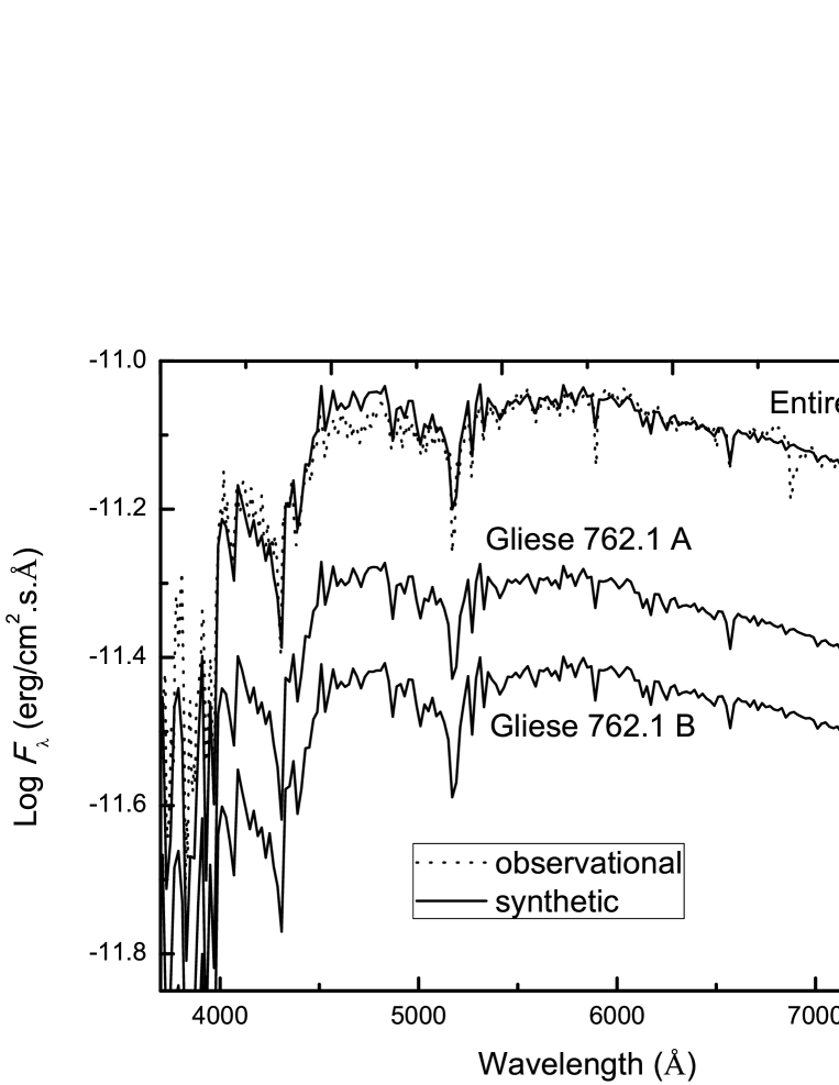
Figure 1: Best fit between the observed entire spectrum (dotted line) which was taken from (Al-Wardat 2002b) and the synthetic entire SED (solid line) for the system Gliese 762.1. Individual synthetic SEDs were computed using $T_{\rm eff}^{A}=5300\pm 50$ K, log $g_{A}=4.56\pm 0.10,R_{A}=0.815\pm 0.09R_{\odot}$, $T_{\rm eff}^{B}=5150\pm 50$ K, log $g_{B}=4.54\pm 0.10$ and $R_{B}=0.806\pm 0.10R_{\odot}$, with $d=16.96$ pc ($\pi=58.96\pm 0.65$ mas).

Table 4: Fundamental parameters of the components of the system Gliese 762.1.

Parameters	Comp. A	Comp. B
$T_{\rm eff}$ (K)	$5300\pm 50$	$5150\pm 50$
Radius (R⊙)	$0.845\pm 0.09$	$0.795\pm 0.10$
$\log g$	$4.52\pm 0.10$	$4.54\pm 0.15$
$L(L_{\odot})$	$0.51\pm 0.08$	$0.40\pm 0.07$
$M_{bol}$	$5\hbox{$.\!\!^{m}$}48\pm 0.90$	$5\hbox{$.\!\!^{m}$}74\pm 1.02$
$M_{V}$	$5\hbox{$.\!\!^{m}$}85\pm 0.80$	$6\hbox{$.\!\!^{m}$}18\pm 0.85$
Mass ($M_{\odot})^{*}$	$0.89\pm 0.08$	$0.83\pm 0.07$
Sp. Type∗∗	K0	K1.5
Parallax (mas)	$58.96\pm 0.65$
($\frac{M_{A}+M_{B}}{M_{\odot}}$)∗∗∗	$1.72\pm 0.60$
Age (Gy)	$9\pm 1$

^∗depending on the equation  5,

^∗∗depending on the tables of Lang (1992),

^∗∗∗depending on the orbital solution.

2.2 Orbital solution and Masses

Once available, the orbital elements of a binary system would enhance and help in examining the physical parameters of its individual components. The mass sum of the two components given by equations  8 and  9 should coincide with that estimated from their positions on the evolutionary tracks and that calculated using the empirical equations and standard tables.

We followed Tokovinin’s method Tokovinin (1992) to calculate the orbital elements. The method performs a least-squares adjustment to all available radial velocity and relative position observations, with weights inversely proportional to the square of their standard errors. The orbital solution involves: the orbital period, P; the semi-amplitudes of the primary and secondary velocities, K1 and K2; the eccentricity, e; the semi-major axis, a; the center of mass velocity, $\gamma$; and the time of primary minimum, $\ T_{0}$. The radial velocities for the system were taken from McClure (1983).

Table 5 lists the results of the radial-velocity solution (Fig. 2). The best orbit passes through the relative position measurements is shown in Fig. 3 and the resulting orbital elements are compared with earlier studies in Table 6.

Table 5: Orbital solution of the system using the velocity curves Fig. 2.

Parameters	McClure (1983)	This paper
$P$, yr	$1.3477\pm 0.0038$	$1.3534\pm 0.0010$
$T_{0},$ MJD	44194.3 $\pm 3.2$	$47670.20\pm 2.01$
$e$	$0.416\pm 0.016$	$0.40\pm 0.013$
$\omega$, deg	$177.1\pm 2.70$	$179.0\pm 2.24$
$K1$, km$s^{-1}$	$9.52\pm 0.16$	$9.40\pm 0.12$
$K2$, km$s^{-1}$	$10.46\pm 0.19$	$10.35\pm 0.19$
$V_{\gamma}$, km$s^{-1}$	$11.41\pm 0.014$	$11.31\pm 0.12$

Table 6: Orbital elements, parallax and total mass of the system Gliese 762.1 using relative position measurements.

Parameters	Arenou et al. (2000)	Pourbaix (2000)	Farrington et al. (2010)	This work
$P$, yr	$1.35458\pm 0.00131$	$1.352776\pm 0.00071$	$1.35297\pm 0.00159$	$1.3534\pm 0.00075$
$T_{0},$ MJD	$48641.21\pm 3.10$	$46164.9\pm 1.66$	$46671.4\pm 8.5$	$47670.20\pm 2.37$
$e$	$0.340\pm 0.013$	$0.3600\pm 0.0078$	$0.371\pm 0.006$	$0.36\pm 0.020$
$a,$ arcsec	$0.084\pm 0.003$	$0.0860\pm 0.0014$	$0.0842\pm 0.3$	$0.0865\pm 0.010$
$i$, deg	$144.6\pm 1.7$	$144\pm 2.4$	$144.0\pm 1.29$	$140.0\pm 2.00$
$\omega$, deg	$177.8\pm 2.1$	$356\pm 2.1$	$16.57\pm 4.1$	$198.0\pm 4.4$
$\Omega$, deg	$74.6\pm 6.8$	$243\pm 1.5$	$256.9\pm 2.666$	$253\pm 6.55$
$\pi$, mas	$57.99\pm 0.57$	$57.3\pm 0.3$	$59.2\pm 2.04$	$58.96\pm 0.65^{a}$
$M,M_{\odot}$	$1.62\pm 0.18$	$1.67\pm 0.83$	$1.59\pm 0.18$	$1.72\pm 0.60$

^a New Hipparcos van Leeuwen (2007) (See Table 1).

Figure 2: Spectroscopic orbital solution for Gliese 762.1 in Table 5 and radial velocities. Triangles represent radial velocities of the primary and squares represent radial velocities of the secondary component. The dotted line in the figure represents the center of mass velocity ( $V_{\gamma}$=$11.31\pm 0.12$ km$s^{-1}$).

Figure 3: The best visual orbit of the system with the relative position measurements from the Fourth Catalog of Interferometric Measurements of Binary Stars. The squares represent the position of the primary component.

The estimated orbital elements, semi-major axis, orbital period (see Table 6), Hipparcos parallax of  van Leeuwen (2007) as $\pi=58.96\pm 0.65$ mas, along with Kepler’s third law:

$$\ M_{A}+M_{B}=(\frac{a^{3}}{\pi^{3}P^{2}})\ M_{\odot}$$ (8)

$$\frac{\sigma_{M}}{M}=\sqrt{(3\frac{\sigma_{\pi}}{\pi})^{2}+(3\frac{\sigma_{a}}{a})^{2}+(2\frac{\sigma_{p}}{p})^{2}}$$ (9)

yield a mass sum with its corresponding error for the system as $\ M_{A}+M_{B}$=$1.72\pm 0.60M_{\odot}$. Using atmospheric modeling equation 5, the total mass of the system is $1.69\pm 0.22M_{\odot}$.

3 SYNTHETIC PHOTOMETRY

The entire and individual synthetic magnitudes are calculated by integrating the model fluxes over each bandpass of the system calibrated to the reference star (Vega) using the following equation Maíz Apellániz (2007); Al-Wardat (2012):

$$m_{p}[F_{\lambda,s}(\lambda)]=-2.5\log\frac{\int P_{p}(\lambda)F_{\lambda,s}(\lambda)\lambda{\rm d}\lambda}{\int P_{p}(\lambda)F_{\lambda,r}(\lambda)\lambda{\rm d}\lambda}+{\rm ZP}_{p}\,,$$ (10)

where $m_{p}$ is the synthetic magnitude of the passband $p$, $P_{p}(\lambda)$ is the dimensionless sensitivity function of the passband $p$, $F_{\lambda,s}(\lambda)$ is the synthetic SED of the object and $F_{\lambda,r}(\lambda)$ is the SED of Vega. Zero points (ZP_p) from Maíz Apellániz (2007) (and references there in) were adopted.

The results of the calculated magnitudes and color indices (Johnson: $U$, $B$, $V$, $R$, $U-B$, $B-V$, $V-R$; Strömgren: $u$, $v$, $b$, $y$, $u-v$, $v-b$, $b-y$ and Tycho: $B_{T}$, $V_{T}$, $B_{T}-V_{T}$) of the entire system and individual components, in different photometrical systems, are shown in Table 7.

Table 7: Magnitudes and color indices of the synthetic spectra of the system Gliese 762.1.

Sys.	Filter	entire	comp.	comp.
		$\sigma=\pm 0.02$	A	B
Joh-	$U$	7.99	8.53	9.01
Cou.	$B$	7.47	8.05	8.43
	$V$	6.60	7.20	7.53
	$R$	6.12	6.74	7.03
	$U-B$	0.52	0.48	0.58
	$B-V$	0.87	0.85	0.90
	$V-R$	0.47	0.46	0.50
Ström.	$u$	9.15	9.69	10.18
	$v$	7.96	8.52	8.94
	$b$	7.06	7.65	8.00
	$y$	6.56	7.16	7.48
	$u-v$	1.19	1.16	1.24
	$v-b$	0.90	0.87	0.94
	$b-y$	0.50	0.49	0.52
Tycho	$B_{T}$	7.71	8.28	8.68
	$V_{T}$	6.70	7.29	7.63
	$B_{T}-V_{T}$	1.02	0.99	1.05

Table 8: Comparison between the observational and synthetic magnitudes, colors and magnitude differences of the system Gliese 762.1.

	Observed †	Synthetic (This work)
$V_{J}$	$6\hbox{$.\!\!^{m}$}60$	$6\hbox{$.\!\!^{m}$}60\pm 0.02$
$B_{J}$	$7\hbox{$.\!\!^{m}$}46$	$7\hbox{$.\!\!^{m}$}47\pm 0.02$
$R_{J}$	$6\hbox{$.\!\!^{m}$}10$	$6\hbox{$.\!\!^{m}$}12\pm 0.02$
$B_{T}$	$7\hbox{$.\!\!^{m}$}71\pm 0.01$	$7\hbox{$.\!\!^{m}$}71\pm 0.02$
$V_{T}$	$6\hbox{$.\!\!^{m}$}71\pm 0.01$	$6\hbox{$.\!\!^{m}$}70\pm 0.02$
$(B-V)_{J}$	$0\hbox{$.\!\!^{m}$}86\pm 0.01$	$0\hbox{$.\!\!^{m}$}87\pm 0.02$
$(U-B)_{J}$	$0\hbox{$.\!\!^{m}$}52\pm 0.02$	$0\hbox{$.\!\!^{m}$}52\pm 0.02$
$\triangle m$	$0\hbox{$.\!\!^{m}$}33^{{\ddagger}}\pm 0.06$	$0\hbox{$.\!\!^{m}$}33\pm 0.04$

${\dagger}$ See Table 1

${\ddagger}$ Average value for fifteen $\triangle m$ measurements (See Table 2).

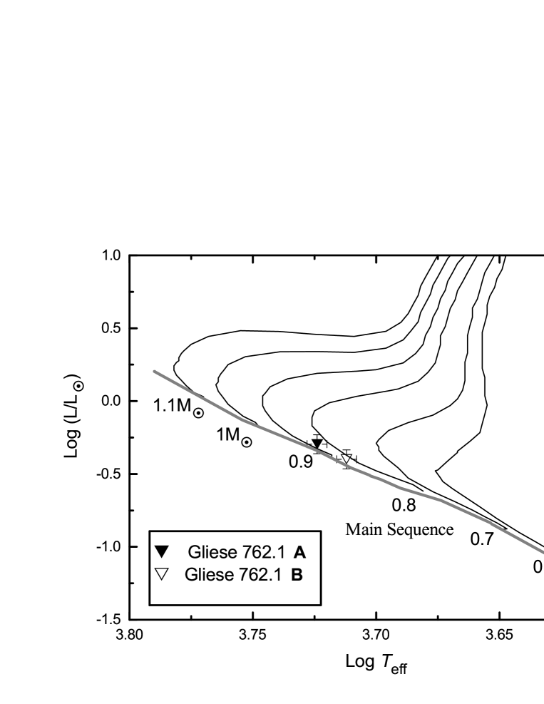
Figure 4: The systems’ components on the evolutionary tracks of masses ( 0.5, 0.6, 0.7,…., 1.1 $M_{\odot}$) of Girardi et al. (2000b).

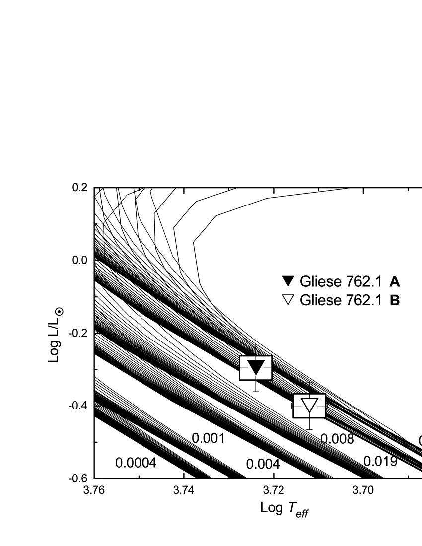
Figure 5: The systems’ components on the isochrones for low- and intermediate-mass stars of different metallicities of  Girardi et al. (2000a).

Figure 6: The systems’ components on the isochrones of low- and intermediate-mass, solar composition [$Z$=0.019, $Y$=0.273] stars of  Girardi et al. (2000a).

4 RESULTS AND DISCUSSION

Table 8 shows a high consistency between the synthetic magnitudes and colors and the observational ones. This gives a good indication about the reliability of the estimated parameters listed in Table 4. Also, the resulted magnitude difference, individual magnitudes and absolute magnitudes (Tables  4& 7) are consistent with the calculated ones as preliminary input parameters.

The positions of the system’s components on the evolutionary tracks of Girardi et al. (2000a) (Fig. 4) show that both components, of mass between $0.8$ and $0.9M_{\odot}$ for each of them, belong to the main-sequence stars, but both show a slight displacement from the zero-age main-sequence upwards. And their positions on  Girardi et al. (2000a) isochrones for low- and intermediate-mass stars of different metallicities and that of the solar composition [$Z=0.019,Y=0.273$] are shown in Figs  5 &  6, which give an age of the system around $9\pm 1$ Gy.

The spectral types and luminosity classes of both components are assigned as K0V and K1.5V for the primary and secondary components respectively, and their positions on the evolutionary tracks are showed in Fig. 4, which are brighter than those given by  Farrington et al. (2010) as K2V and K4V.

The estimated orbital elements of the system (Tables 5 & 6) are consistent with previous works. The orbit of the system was solved using a combination of the relative position measurements and the radial velocity curves, which gives more reliable and accurate results.

The mass sum of the system components and the individual masses were calculated and estimated in three different ways; using the physical parameters and standard relations as $M_{a}=0.89\pm 0.08M_{\odot},M_{b}=0.83\pm 0.07M_{\odot}$, using the orbital elements with Hipparcos parallax as $M_{a}+M_{b}=1.72\pm 0.60M_{\odot}$ and depending on the positions of the system’s components on the evolutionary tracks of Girardi et al. (2000a) (Fig. 4) which coincide with the calculated ones.

Depending on the estimated parameters of the system’s components and their positions on the evolutionary tracks, fragmentation is a possible process for the formation of the system. Where Bonnell (1994) concludes that fragmentation of a rotating disk around an incipient central protostar is possible, as long as there is continuing infall. Zinnecker & Mathieu (2001) pointed out that hierarchical fragmentation during rotational collapse has been invoked to produce binaries and multiple systems.

It is worthwhile to mention here that the system Gliese 762.1 is a detached one with an orbital period of $1.3534\pm 0.0010$yr. So, this system is a visually close but not a contact binary, and if we compare it with other extremely K-type close binary systems like BI Vulpeculae  (Qian et al. 2013), AD Cancri  (Qian et al. 2007) and PY Virginis  (Zhu et al. 2013), which have shorter orbital periods ( days) and lower angular momentum among K-type binary stars, we find that the orbital evolution of such systems are affected by the existence of a third component by removing angular momentum from the central binary system during the early stellar formation process or/and later dynamical interactions. However, as for Gliese 762.1, such dynamical interactions may not exist. It may form directly from stellar formation process because the orbital separation between the two components is much larger.

5 CONCLUSIONS

We present the results of the complex analysis of the double-lined spectroscopic binary system Gliese 762.1. We were able to achieve the best fit between the entire synthetic SED’s and the observational one (Fig. 1) by producing and calibrating synthetic SED of the individual components in an iterated method. The orbit of the system and its radial velocities were also solved to estimate reliable orbital elements consistent with the physical ones of atmospheres modeling.

We relayed on Hipparcos parallax ($58.96\pm 0.65$ mas, $d=16.96$ pc van Leeuwen (2007)) for the calculations of the entire SED and the masses of the system. The Hipparcos parallax was not that far from the dynamical parallaxes introduced in previous orbital solutions (see Table 6).