On the Accuracy of the Padé–Resummed Master Equation Approach to Dissipative Quantum Dynamics

Abstract

Well–defined criteria are proposed for assessing the accuracy of quantum master equations whose memory functions are approximated by Padé resummation of the first two moments in the electronic coupling. These criteria partition the parameter space into distinct levels of expected accuracy, ranging from quantitatively accurate regimes to regions of parameter space where the approach is not expected to be applicable. Extensive comparison of Padé–resummed master equations with numerically exact results in the context of the spin–boson model demonstrate that the proposed criteria correctly demarcate the regions of parameter space where the Padé approximation is reliable. The applicability analysis we present is not confined to the specifics of the Hamiltonian under consideration and should provide guidelines for other classes of resummation techniques.

I Introduction

The study of open quantum systems is among the most active areas in condensed matter science.Leggett et al. (1987) Under the rubric of dissipative quantum dynamics falls topics ranging from electron and energy transferEngel et al. (2007); Lee, Cheng, and Fleming (2007); Panitchayangkoon et al. (2010); Collini and Scholes (2009); Brédas and Silbey (2009) to singlet fission dynamics in condensed media.Smith and Michl (2010); Teichen and Eaves (2012); Berkelbach, Hybertsen, and Reichman (2013a, b, 2014) The theoretical treatment of the dynamics of open quantum systems is challenging due to the large number of degrees of freedom and energy scales in such problems. Numerically exact approachesMakarov and Makri (1994); Makri (1995); Makri and Makarov (1995a, b); Mak and Egger (2007); Wang, Thoss, and Miller (2001); Wang and Thoss (2003); Tanimura and Kubo (1989); Ishizaki and Fleming (2009a); Strümpfer and Schulten (2012); Zhang and Yan (2016) are generally limited to idealized models, while approximate approachesTully (1998, 2012); Thoss, Wang, and Miller (2001); Berkelbach, Reichman, and Markland (2012); Montoya-Castillo, Berkelbach, and Reichman (2015) are often limited by issues of both accuracy and scalablility. Thus, the search for methods that are reliable, general, and numerically efficient continues at the forefront of theoretical chemistry and physics.

Schemes based on projection operator techniquesGrabert (1982) and generalized quantum master equations (GQMEs) have been used both to design successful approximate approaches and as a platform to develop numerically exact methods.Bloch (1957); Tanimura and Kubo (1989); Redfield (1965); Weiss (1999); Nitzan (2006) The projection operator technique partitions the Hilbert space into system and bath subspaces, leading to the derivation of GQME for the system subspace which accounts for the bath’s dynamical influence on the system via a memory kernel. Exact and approximate techniques for the evaluation of the memory kernel have been developed that make use of perturbation theories,Leggett et al. (1987); Würger (1997); Zhang et al. (1998); Yang and Fleming (2002); Ishizaki and Fleming (2009b) resummation techniques,Sparpaglione and Mukamel (1988a, b); Golosov and Reichman (2001a, b, 2004); Mavros and Van Voorhis (2014) and self–consistent expansions.Shi and Geva (2003, 2004); Cohen and Rabani (2011); Cohen, Wilner, and Rabani (2013) Recent progress afforded by these methods has illustrated several advantages of the GQME scheme. First, the memory kernel may decay on a shorter timescale than the system dynamics under study, so that approximate memory kernels may yield more accurate dynamics than would be obtained by direct simulation of the system dynamics using the same level of approximation. Second, the GQME scheme is general enough to treat realistic anharmonic bathsShi and Geva (2004); Golosov and Reichman (2001b) and arbitrary system–bath coupling.Shi and Geva (2004) Finally, the flexibility of different projection operator formulations allows for facile extension to more general situations, such as nonequilibrium initial preparation,Evans and Coalson (1995); Coalson, Evans, and Nitzan (1994) as well as more complex correlation functions.Montoya Castillo and Reichman (2016) However, despite these notable results, it remains a difficult task to accurately calculate memory kernels in many regimes of general quantum dissipative systems.

The Padé resummation approach approximates the memory kernel as an infinite resummation based on the kernel’s second and fourth moments.Basdevant (1972); Sparpaglione and Mukamel (1988a) At the expense of fourth–order perturbation theory in the electronic coupling, the Padé–resummed GQME is capable of producing an accuracy that exceeds that of simple perturbation theory for the spin–boson model,Golosov and Reichman (2004) and resummation of higher order kernels provide quantitative corrections.Gong et al. (2015) Recently, however, it has been demonstrated that this approach can lead to unphysical, divergent dynamics in the strong electronic coupling regime,Mavros and Van Voorhis (2014) and the applicability and accuracy of the Padé approximations throughout the entire parameter space is still difficult to evaluate. The aim of the present work is to provide feasible estimates of the applicability based on analysis of the Padé approximation itself.

We propose well–defined criteria in terms of the kernel’s second and fourth moments that correspond to conditions leading to “physically reasonable” results within the Padé resummation scheme. To examine the proposed criteria, we perform systematic benchmark comparisons of Padé–resummation with numerically exact results for a prototypical dissipative open quantum system, namely the spin–boson model with a Debye spectral density. The proposed criteria divide the parameter space into subspaces associated with different levels of accuracy, and we confirm that the systematic comparison of population dynamics with exact results clearly demarcate when the approach should provide quantitatively reliable results. It should be noted that the proposed criteria are not limited to the spin–boson model, but are generally applicable for estimating the accuracy of Padé–resummed memory kernels for generic open quantum systems. In addition, the present work may provide guidelines for the applicability of other types of resummation techniques, such as the Landau–Zener resummation.Mavros and Van Voorhis (2014)

The outline of the paper is as follows. We present in Sec. II a brief review of the nonequilibrium Padé–resummed GQME approach to a generic open quantum system. In Sec. III, we analyze the Padé resummation and define the criteria for the validity of the approximation. We apply the proposed criteria to the spin–boson model in Sec. IV and show the correspondence of the different regions of the applicability phase diagrams with exactly computed population dynamics. In Sec. V, we conclude.

II The Padé resummed GQME approach

We consider an open quantum system whose Hamiltonian takes the form, $\hat{H}=\hat{H}_{s}+\hat{H}_{b}+\hat{V}$, where $\hat{H}_{s}$ and $\hat{H}_{b}$ correspond to the system and bath Hamiltonians, respectively, and $\hat{V}$ denotes the system–bath coupling. We denote the quantum states of the system by the kets $\left|j\right\rangle$ and the bath density operator by $\hat{\rho}$. It is convenient to adopt the Liouville space notationSparpaglione and Mukamel (1988a, b) for the total density operator, $\hat{W}\equiv|W\rangle\rangle$, and define the product $\langle\langle A|B\rangle\rangle\equiv\text{Tr}_{s}\text{Tr}_{b}\{A^{\dagger}B\}$ where $\text{Tr}_{s}$ and $\text{Tr}_{b}$ are partial traces over the states of the system and bath, respectively. Time evolution of the density operator is governed by the Liouville–von Neumann equation

$$\frac{d}{dt}|W(t)\rangle\rangle=-i\mathcal{L}|W(t)\rangle\rangle,$$ (1)

where the Liouville super–operator (the Liouvillian) is defined by $\mathcal{L}|W(t)\rangle\rangle=[\hat{H},\hat{W}(t)]$ and we set $\hbar=1$ throughout this paper. The reduced density matrix of the system can be written as $\sigma_{jk}(t)=\text{Tr}_{b}\left\{\left|k\right\rangle\left\langle j\right|W(t)\right\}=\langle\langle jk|W(t)\rangle\rangle$ where the Liouville state is given by $|jk\rangle\rangle=\left|j\right\rangle\left\langle k\right|\otimes\hat{1}$ and $\hat{1}$ is the unit operator for the bath. Then we can denote the population dynamics as

$$P_{j}(t)=\langle\langle j|W(t)\rangle\rangle,$$ (2)

where the diagonal elements are expressed as $|jj\rangle\rangle\rightarrow|j\rangle\rangle$ for simplicity.

We implement the standard projection operator techniqueZwanzig (1961) via the super–operator

$$\mathcal{P}=\sum_{j}|j\rho_{j}\rangle\rangle\langle\langle j|$$ (3)

where $|j\rho_{j}\rangle\rangle=\left|j\right\rangle\left\langle j\right|\otimes\hat{\rho}_{j}$ and the bath density operator $\hat{\rho}_{j}$ is taken to be in equilibrium in the electronic state $\left|j\right\rangle$. The projected version of Eq. (1) yields the GQME for the population of the $j$-th state,

$$\frac{d}{dt}P_{j}(t)=\mathcal{I}_{j}(t)-{\color[rgb]{1,0,0}\sum_{k}}\int_{0}^{t}d\tau\mathcal{K}_{jk}(t-\tau)P_{k}(\tau),$$ (4)

where the memory kernel matrix is

$$\mathcal{K}_{jk}(t)=\langle\langle j|\mathcal{P}\mathcal{L}e^{-i\mathcal{Q}\mathcal{L}t}\mathcal{Q}\mathcal{L}|k\rho_{k}\rangle\rangle,$$ (5)

and the inhomogeneous terms are given by

$$\mathcal{I}_{j}(t)=-i\langle\langle j|\mathcal{P}\mathcal{L}e^{-i\mathcal{Q}\mathcal{L}t}\mathcal{Q}|W(0)\rangle\rangle,$$ (6)

with $\mathcal{Q}=1-\mathcal{P}$. The inhomogeneous terms result from the fact that the initial condition for the total density operator will generally satisfy $\mathcal{Q}|W(0)\rangle\rangle\neq 0$. For cases $\mathcal{Q}|W(0)\rangle\rangle=0$, $\mathcal{I}_{j}(t)=0$. In the frequency domain, Eq. (4) can be transformed from an integro–differential equation into the algebraic form

$$sp_{j}(s)=p_{j}(t=0)+I_{j}(s)-\sum_{k}K_{jk}(s)p_{k}(s)$$ (7)

with the use of the one–side Laplace transformation, $f(s)=\int_{0}^{\infty}e^{-st}F(t)dt$, where $s$ is a complex number. It should be noted that calculation of the memory kernel matrix and the inhomogeneous terms is difficult in part because dynamical evolution involves a projected propagator $e^{-i\mathcal{Q}\mathcal{L}t}$.

To approximate the projected propagator, one can carry out a perturbation treatment with respect to a perturbation $\hat{H}^{\prime}$ and an unperturbed Hamiltonian $\hat{H}_{0}=\hat{H}-\hat{H}^{\prime}$. The Liouvillian can be decomposed as $\mathcal{L}=\mathcal{L}_{0}+\mathcal{L}^{\prime}$ and Eq. (5) and (6) can be expanded in terms of $\mathcal{L}^{\prime}$. As a result, the memory matrix and the inhomogeneous terms in frequency domain can be expressed as a moment expansion $K_{jk}(s)=\sum_{n=1}^{\infty}K_{jk}^{(2n)}(s)$ and $I_{j}(s)=\sum_{n=1}^{\infty}I_{j}^{(2n)}(s)$ with

$$K_{jk}^{(2n)}(s)=\langle\langle j|\left[\mathcal{L}^{\prime}G_{0}(s)\mathcal{L}^{\prime}G_{0}(s)\mathcal{Q}\right]^{n-1}\mathcal{L}^{\prime}G_{0}(s)\mathcal{L}^{\prime}|k\rho_{k}\rangle\rangle,$$ (8)

and

$$I_{j}^{(2n)}(s)=\langle\langle j|\mathcal{L}^{\prime}G_{0}(s)[\mathcal{Q}\mathcal{L}^{\prime}G_{0}(s)]^{2n-1}\mathcal{Q}|W(0)\rangle\rangle,$$ (9)

where the unperturbed Green’s function is $G_{0}(s)=\left(s+i\mathcal{L}_{0}\right)^{-1}$. In practice, evaluating the $(2n)$-th order moment requires a Laplace transformation for each time variable in a $(2n-1)$-time correlation function. Clearly, the complexity of the terms in the moment expansion grows quickly as the moment order increases.

The memory matrix and inhomogeneous terms may be approximated by a Padé resummation using the second and fourth moments in the frequency domain,

$$K_{jk}(s)\approx\frac{[K_{jk}^{(2)}(s)]^{2}}{K_{jk}^{(2)}(s)-K_{jk}^{(4)}(s)},$$ (10)

$$I_{j}(s)\approx\frac{[I_{j}^{(2)}(s)]^{2}}{I_{j}^{(2)}(s)-I_{j}^{(4)}(s)}.$$ (11)

It should be noted that the Padé resummation is a rational expression that include infinite orders of the perturbation $\hat{H}^{\prime}$, but the contributions of higher order than the fourth are approximated; for example, $K_{jk}^{(6)}\approx\left[K_{jk}^{(4)}(s)\right]^{2}/K_{jk}^{(2)}(s)$. The expressions of this section have been discussed before,Golosov and Reichman (2001b) but a systematic analysis is lacking. We now focus precisely on this issue.

III Applicability Analysis and criteria

The accuracy of the Padé resummation is unknown and depends on the analyticity of an unknown function in the complex plane. Despite this fundamental difficulty, we may estimate its validity via simple convergence properties and physical requirements of the memory kernels. For simplicity below, the criteria are expressed in terms of a single memory kernel element $K(s)$, thereby suppressing the indices associated with memory functions and inhomogeneous terms.

The Padé resummation can be viewed as a complex geometric series which is expected to yield well–behaved results only within the disk of convergence of the Laurent series that represents the expansion in the complex plane. A necessary condition for such convergence is $\|K^{(4)}(s)/K^{(2)}(s)\|<1$, for all $s\in\mathbb{C}$, where $K^{(n)}(s)$ is the $n$-th order expression given in Eq. (8). Since the inverse Laplace transformation is performed along the imaginary axis $s=i\omega$, we restrict this condition to

$$\text{(a)}\qquad\qquad\|K^{(4)}(i\omega)/K^{(2)}(i\omega)\|<1\text{~{}for real }\omega.\qquad\qquad$$

The above condition is quite strict and may be relaxed by consideration of the physical requirements of a generic memory kernel. Consider the Laplace inversion via the contour integration of the Bromwich integral $K(t)=\frac{1}{2\pi i}\int_{\mathcal{C}}K(s)e^{st}ds$, where $\mathcal{C}$ is the vertical contour in the complex plane chosen to include all singularities of $K(s)$ to the left of it. Arfken (2013); Yonemoto, Hisakado, and Okumura (2003) The asymptotic physical behavior of the memory kernel dictates that the poles of the Padé–resummed approximation cannot have a non–negative real part, otherwise the memory function would not be guaranteed to decay to zero as $t\rightarrow\infty$. We assume that the distribution of poles changes continuously and smoothly as the parameters of the model changes, allowing us to focus on the imaginary axis $s=i\omega$ and monitor the behavior of $K^{(4)}(i\omega)/K^{(2)}(i\omega)$. In particular, the equality $\text{Re}[K^{(4)}(i\omega^{*})/K^{(2)}(i\omega^{*})]=1$ is a necessary (albeit not sufficient) condition for the occurrence of a pole on the imaginary axis at $s=i\omega^{*}$, which obviate the asymptotic decay of the memory kernel in real–time. We thus propose a second condition

$$\text{(b)}\qquad\qquad\text{Re}[K^{(4)}(i\omega)/K^{(2)}(i\omega)]<1\ \text{for real }\omega,\qquad\qquad$$

which, excepting random occurrences, maintains that all poles are confined to the left of the imaginary axis in the complex plane and that the memory function is well behaved. Note that the first criterion is stricter than the second since it corresponds to the interior of a unit circle in the complex plane while the latter condition corresponds to the entire complex plane to the left of the boundary at $\text{Re}[z]=1$.

These criteria are indeed crude because they rely on the the limited information of the first two terms of an infinite expansion. We will employ these conditions below as demarcation lines in parameter space to gauge the reliability of the Padé approximation. As will be demonstrated, the criteria provide robust if conservative guidelines for the domain of applicability for Padé–resummed master equations.

IV Results for the spin–boson model

IV.1 Padé–resummed GQME approach for the spin–boson model

In this section, we examine the criteria suggested above via investigation of the population dynamics in the spin–boson model. The spin–boson model is an idealization of an open quantum system which contains most of the important generic features of more complicated dissipative quantum systems while offering the advantage that numerically exact algorithms exist for the calculation of its dynamics over a wide range of parameter space.Tanimura and Kubo (1989); Makarov and Makri (1994); Makri (1995); Thoss, Wang, and Miller (2001) To produce benchmark results for the spin–boson model in this work, we use the numerically exact hierarchical equations of motion (HEOM) methodology in the Parallel Hierarchy Integrator (PHI).Strümpfer and Schulten (2012)

We consider a two–level system with energy bias $\epsilon$ and constant electronic coupling $\Delta$

$$\hat{H}_{s}=\frac{\epsilon}{2}\hat{\sigma}_{z}+\Delta\hat{\sigma}_{x},$$ (12)

and $\hat{\sigma}_{z}=\left|1\right\rangle\left\langle 1\right|-\left|2\right\rangle\left\langle 2\right|$ and $\hat{\sigma}_{x}=\left|1\right\rangle\left\langle 2\right|+\left|2\right\rangle\left\langle 1\right|$. The two–level system is coupled to a bath consisting of an infinite set of harmonic oscillators

$$\hat{H}_{b}=\sum_{\alpha}\frac{\hat{P}_{\alpha}^{2}}{2}+\frac{1}{2}\omega_{\alpha}^{2}\hat{Q}_{\alpha}^{2}.$$ (13)

Here, the frequency of the $\alpha$-th bath mode is $\omega_{\alpha}$, while $\hat{P}_{\alpha}$, $\hat{Q}_{\alpha}$ refer to the mass–weighted momenta and coordinates of the $\alpha$-th mode. The system–bath coupling is taken to be of the form

$$\hat{V}=\hat{\sigma}_{z}\sum_{\alpha}c_{\alpha}\hat{Q}_{\alpha},$$ (14)

where $c_{\alpha}$ is the coupling strength between the two–level system and the $\alpha$-th harmonic oscillator. The spectral density compactly describes the influence of the bath on the dynamics of the system, and takes the form

$$J(\omega)=\frac{\pi}{2}\sum_{\alpha}\frac{c_{\alpha}^{2}}{\omega_{\alpha}}\delta(\omega-\omega_{\alpha}).$$ (15)

In our study we choose the commonly used Debye spectral densityThoss, Wang, and Miller (2001)

$$J(\omega)=\frac{\lambda}{2}\frac{\omega\omega_{c}}{\omega^{2}+\omega_{c}^{2}},$$ (16)

which is Ohmic at low frequency with a Lorentzian cutoff at high frequency. The Debye spectral density is characterized by two parameters: the characteristic bath frequency $\omega_{c}$, which represents the average timescale of the bath response, and the reorganization energy $\lambda=\sum_{\alpha}c_{\alpha}^{2}/2\omega_{\alpha}^{2}$, which is a direct measure of the coupling strength between the system and the bath. In electron–transfer theory, the Debye spectral density is commonly used for the description of a solvent environment with Debye dielectric relaxation (i.e. exponential in time).

Throughout this work, we employ an initial density operator for the bath of the form

$$\hat{\rho}_{0}=\frac{e^{-\beta\hat{H}_{b}}}{\text{Tr}_{b}\{e^{-\beta\hat{H}_{b}}\}},$$ (17)

where $\beta=1/k_{B}T$ is the inverse temperature of the bath. This initial condition corresponds to thermal equilibrium in the reservoir in the absence of the system–bath coupling and is the initial density operator of relevance for the description of an impulsive Franck–Condon excitation.

We implement a commonly used projection operator of the form,Sparpaglione and Mukamel (1988a, b)

$$\mathcal{P}=|1\rho_{1}\rangle\rangle\langle\langle 1|+|2\rho_{2}\rangle\rangle\langle\langle 2|,$$ (18)

where fully–dressed equilibrium bath density operators of the form

$$\hat{\rho}_{j}=\frac{e^{-\beta\hat{H}_{j}}}{\text{Tr}_{b}\{e^{-\beta\hat{H}_{j}}\}}$$ (19)

are employed with $\hat{H}_{j}=\pm(\frac{\epsilon}{2}+\sum_{\alpha}c_{\alpha}\hat{Q}_{\alpha})+\hat{H}_{b}$ ($+$ for $1$ and $-$ for $2$). Note that with the use of the projector (18), factorized initial conditions with an uncorrelated bath (17) will necessitate the evolution of inhomogeneous terms (11) in the GQME. The second–order moments of the memory kernels ($K_{jk}^{(2)}$) result in an expression equivalent to the noninteracting blip approximation (NIBA).Weiss (1999) We carry out the time integrations of the memory kernels and the inhomogeneous terms by the techniques outlined in Ref. Golosov and Reichman, 2004 and the same Gaussian quadrature subroutine (DCUTRI).Berntsen, Espelid, and Genz (1991) The population dynamics of the Padé–resummed GQME is calculated via the accuracy–improved numerical method for Laplace inversion.Yonemoto, Hisakado, and Okumura (2003)

For this spin–boson model, the Padé–resummed GQME approach has lead to population dynamics in near perfect agreement with numerically exact simulations.Golosov and Reichman (2001a, 2004) On the other hand, Van Voorhis and coworkers have shown the breakdown of the Padé–resummed GQME approach in the strong electronic coupling region.Mavros and Van Voorhis (2014) Our goal in the following is to systematically delineate the regime of validity of the approach based on the criteria of Sec III.

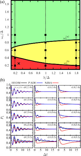
Figure 1: Parameter space diagram for the spin–boson model with zero bias ($\epsilon=0$) and at high temperature ($k_{B}T=2\Delta$). The critical frequencies $\omega_{c}^{(a)}$ and $\omega_{c}^{(b)}$ are indicated as functions of $\lambda$. The green region ($\omega_{c}>\omega_{c}^{(a)}$) is the regime where dynamics are expected to be quantitatively accurate, the yellow region ($\omega_{c}^{(b)}<\omega_{c}<\omega_{c}^{(a)}$) is the regime where dynamics are expected to be semi–quantitatively accurate and the red region ($\omega_{c}<\omega_{c}^{(b)}$) is the regime where the Padé–resummed approach is expected to be unreliable or even unstable. The lower panels are the corresponding population dynamics along the vertical cuts (indicated as solid squares connected by dashed lines) calculated by the HEOM approach (red solid lines), Padé–resummed GQME (PADE, green dash lines), and NIBA (blue doted lines). The upper right label in each population dynamics panel denotes the value of $(\lambda,\omega_{c})/\Delta$. The symbol $\boldsymbol{\times}$ in the phase diagram refers to the parameters corresponding to Fig. 1(d) of Ref. Mavros and Van Voorhis, 2014.

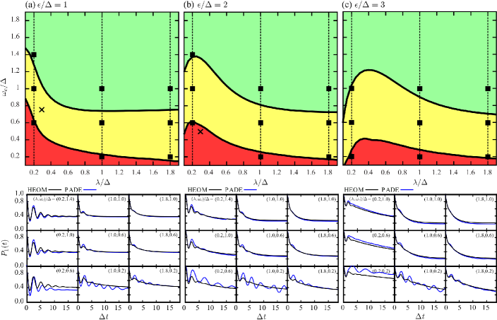
Figure 2: Parameter space diagram with increasing bias energies $\epsilon/\Delta=1,\ 2,\ 3$ at high temperatures ($k_{B}T=2\Delta$) for the spin–boson model. The critical frequencies $\omega_{c}^{(a)}$ and $\omega_{c}^{(b)}$ are indicated as functions of $\lambda$ with color regions as in Fig. 1. The lower panels are the corresponding population dynamics along the vertical cuts calculated by the HEOM approach (red solid line) and the Padé–resummed GQME (PADE, green dash line). The upper right label in each population dynamics plot denotes the value of $(\lambda,\omega_{c})/\Delta$. The symbol $\boldsymbol{\times}$ in panel (a) refers to the parameters corresponding to Fig. 3(b) of Ref. Mavros and Van Voorhis, 2014, while that in panel (b) corresponds to Fig. 4(b) of Ref. Mavros and Van Voorhis, 2014.

IV.2 Parameter Space Diagrams

The model we study in this work can be parametrized by five independent energy scales. We use the electronic coupling $\Delta$ as the unit of energy so that four dimensionless parameters characterize the parameter space. These are: the electronic bias $\epsilon/\Delta$, the reorganization energy $\lambda/\Delta$, the bath’s characteristic frequency $\omega_{c}/\Delta$, and the thermal energy of the bath $k_{B}T/\Delta$.

To systematically scan parameter space, we consider variation in the scaled $\omega_{c}$–$\lambda$ plane for different scaled temperature and bias cuts. It is expected that, for a given system–bath coupling $\lambda$, smaller values of $\omega_{c}/\Delta$ render the Padé approximation less accurate due to the fact that the perturbation series is ordered by $\Delta$. Therefore, we define critical characteristic frequencies, $\omega_{c}^{(a)}(\lambda)$ and $\omega_{c}^{(b)}(\lambda)$, as the lower bound of scaled $\omega_{c}$ to satisfy the criteria (a) and (b) for all elements of the memory kernels respectively. The boundaries $\omega_{c}^{(a)}(\lambda)$ and $\omega_{c}^{(b)}(\lambda)$ are determined by the conditions that there exists a single imaginary number $i\omega^{*}$ for which either

$$\qquad\text{(a)}\qquad\quad\|K^{(4)}(i\omega^{*})/K^{(2)}(i\omega^{*})\|=1,\qquad\qquad\qquad$$

or

$$\qquad\text{(b)}\qquad\text{Re}[K^{(4)}(i\omega^{*})/K^{(2)}(i\omega^{*})]=1,\qquad\qquad\qquad$$

is satisfied. The critical characteristic frequencies indicate the boundaries of the proposed criteria that partition parameter space into three distinct regions of different levels of accuracy.

Because $K(t)$ and $I(t)$ have similar structure that should decay to zero after a transient time and the Padé approximation takes the same form for both $K(s)$ and $I(s)$, we expect the proposed criteria also apply to the inhomogeneous term. In fact, Refs. Golosov and Reichman, 2001a–Golosov and Reichman, 2004 have shown that the initial preparation of the bath, captured by the inhomogeneous term, is crucial for obtaining the correct dynamics. We only focus here on the memory kernel and expect the inhomogeneous term have similar analytical behaviors.

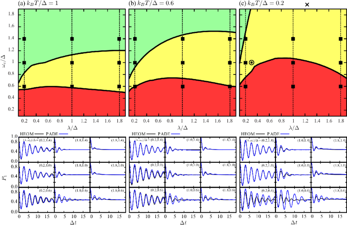
Figure 3: Parameter space diagrams with zero bias energy ($\epsilon=0$) as a function of decreasing temperature $k_{B}T/\Delta=1.0,\ 0.6,\ 0.2$ from left to right. The critical frequencies $\omega_{c}^{(a)}$ and $\omega_{c}^{(b)}$ are indicated as functions of $\lambda$ with color regions as in Fig. 1. The lower panels are the corresponding population dynamics along the vertical cuts calculated by the HEOM approach (red solid line) and Padé–resummed GQME (PADE, green dash line). The upper right label in each population dynamics panel denotes the value of $(\lambda,\omega_{c})/\Delta$. The symbol $\boldsymbol{\times}$ in panel (c) refers to the parameters corresponding to Fig. 2(b) of Ref. Mavros and Van Voorhis, 2014. The symbol $\odot$ indicates the same $(\lambda,\omega_{c})$ of Fig. 3(c) of Ref. Mavros and Van Voorhis, 2014, but with $\epsilon=0$.

For illustrative purposes, we show a phase diagram for an unbiased ($\epsilon=0$), high temperature ($k_{B}T=2\Delta$) system in Fig. 1 and the corresponding population dynamics of selected points in parameter space calculated by the HEOM, Padé and NIBA approaches in the lower panels. For this example the three regions may be partitioned as:

1. $\omega_{c}>\omega_{c}^{(a)}$ (quantitatively accurate):

   In this regime, the results of the Padé approach achieve almost perfect agreement with the numerically exact results. This regime covers the weak electronic coupling (non–adiabatic) limit ($\omega_{c}/\Delta\gg 1$), where the $\Delta$–perturbation based methods works well. We also find that the Padé–resummed approach provides a significant improvement over NIBA in the large system–bath coupling regime, as can be seen in the upper panels of Fig. 1 (b).

2. $\omega_{c}^{(b)}<\omega_{c}<\omega_{c}^{(a)}$ (semi–quantitatively accurate):

   The population dynamics of the Padé approach in this region are not quite as accurate as in the “quantitatively accurate” regime, but the Padé–resummed method still captures most of the important features in a semi–quantitative manner, such as the long–lived oscillations and dissipative relaxation. Since the electronic coupling is considered to be intermediate, the NIBA results become worse while the Padé results remain accurate.

3. $\omega_{c}<\omega_{c}^{(b)}$ (unreliable):

   The discrepancies in the population dynamics between the Padé approach and the HEOM generally become larger in this regime since the large electronic coupling ($\Delta/\omega_{c}\gg 1$) renders the perturbation theory in $\Delta$ questionable. In this regime, the Padé approach may lead to a shift of the oscillation frequency of the population (see panels labeled by $(\lambda,\omega_{c})/\Delta=(0.2,0.4),\ (0.2,0.2),\ (1.8,0.2)$), as well as overly coherent behavior (see the panel labeled by $(\lambda,\omega_{c})/\Delta=(1.0,0.2)$). Extreme cases in the strong electronic coupling (adiabatic) limit may cause the Padé resummation breakdown and result in unphysical population dynamics. Importantly, the parameters of Fig. 1(d) of Ref. Mavros and Van Voorhis, 2014 lie in the “unreliable” region (labeled by $\boldsymbol{\times}$ in the phase diagram). In this case the Padé–resummed approach yields unphysical population dynamics for the long time behavior.

IV.3 Energetic bias dependence

The bias dependence of the parameter space phase diagram is shown in Fig. 2, as well as the corresponding population dynamics. We find that, as the energetic bias grows, both critical frequencies increase in the low $\lambda$ region. Furthermore, in the region when $\omega_{c}<\omega_{c}^{(b)}$, the Padé approach may lead to incorrect steady state population values (see the panels labeled $(\lambda,\omega_{c})/\Delta=(0.2,0.6)$ for $\epsilon=\Delta$ and $(\lambda,\omega_{c})/\Delta=(0.2,0.2)$ for $\epsilon=3\Delta$) as well as an unphysical “recoherence” behavior (namely the envelope of the population does not decay monotonically) as illustrated in the panels $(\lambda,\omega_{c})/\Delta=(1.0,0.2)$ for all biases. This effect can be attributed to near singularities in the approximate kernels when the Padé resummation does not satisfy the criterion (b). The population dynamics in Fig. 3(b) and Fig. 4(b) of Ref. Mavros and Van Voorhis, 2014 show qualitatively similar discrepancies from exact calculations as illustrated here.Note (1) The parameters for these two cases (labeled as $(\times)$ in Fig. 2) lie in the expected regions of parameter space.

We find that $\omega_{c}^{(a)}$ and $\omega_{c}^{(b)}$ become insensitive to the energetic bias in the limit $\lambda\gg\epsilon$. Since the reorganization processes dominate the incoherent decay in this limit, the fluctuations induced by the energetic bias becomes less important here. Hence, the boundaries of accuracy of the Padé–resummed GQME approach do not change when system–bath coupling becomes very large.

IV.4 Temperature dependence

In general, the Padé–resummed GQME approach becomes less accurate for lower temperature baths. Fig. 3 shows that, as the temperature decreases, the critical frequencies increase significantly throughout the entire range of reorganization energies. This may be explained by the fact that the bath degrees of freedom progressively populate lower frequency modes as temperature decreases, rendering $\Delta$ relatively larger with respect to the participating low–frequency modes. However, the Padé approach can still properly capture the dynamical effect of the bath and yield qualitatively reasonable results in the semi–quantitatively accurate region.

In the regions of lower accuracy, the Padé approach tends to overestimate the coherent oscillations. In addition, the coherent oscillations are generally shifted toward lower frequencies. In addition, we observe spurious recoherence in the panel labeled $(\lambda,\omega_{c})/\Delta=(1.0,0.6)$ for $k_{B}T=0.2\Delta$. Once again the most sever deviations from exact calculation are found in the region $\omega_{c}<\omega_{c}^{(b)}(\lambda)$ as expected.

The value $(\lambda,\omega_{c})/\Delta=(1.0,0.3)$ of Fig. 3(c) of Ref. Mavros and Van Voorhis, 2014 is labeled ($\odot$) in panel (c) of Fig. 3. However, note that the values of the energetic bias are different in this comparison. As discussed above, we expect both critical frequencies to increase in the low $\lambda$ region as the value of bias grows. Hence, we infer by this trend that the value of $(\lambda,\omega_{c})/\Delta$ in the biased case should lie in the region of parameter space where the Padé approach is expected to be unreliable.

V Conclusions

In this work we provide criteria to estimate the accuracy and applicability of the nonequilibrium Padé–resummed GQME approach to dissipative quantum dynamics. For the spin–boson model, the criteria yield critical frequencies $\omega_{c}^{(a)}(\lambda)$ and $\omega_{c}^{(b)}(\lambda)$ that partition the parameter space into three distinct regions of expected accuracy. One particularly significant outcome of our analysis is the fact that the difficult intermediate coupling regime, where all energy scales are comparable, falls frequently into a region of parameter space where the Padé approach is expected to be accurate, and indeed we find that the Padé–resummed GQME can still capture significant features of population dynamics within this regime. When $\omega_{c}<\omega_{c}^{(b)}(\lambda)$, the Padé–resummed GQME is demonstrated to often exhibit spurious long–time behavior, overestimate oscillations with shifted frequencies, and display unphysical recoherence. Overall, we find that the accuracy of the Padé resummation is relatively insensitive to the system bias and reorganization energy, but becomes worse with decreasing bath frequency and decreasing temperature.

The criteria of accuracy we propose is crude for several reasons. First, it is only based on the analytic properties of the first two moments of an infinite expansion. Second, even with regard to these moments, we merely search for the boundaries in the complex plane where a single pole may obviate physical properties required of generic memory functions. In this sense, the boundaries of accuracy are conservative and we expect to see cases where the Padé approach may still yield accurate results even if $\omega_{c}^{(b)}(\lambda)<\omega_{c}<\omega_{c}^{(a)}(\lambda)$ and even occasionally when $\omega_{c}<\omega_{c}^{(b)}(\lambda)$ . Indeed, we do find cases where exact calculations demonstrate that the approximate results may be more accurate than expected. However, overall we find that the trends predicted by the criteria of Sec. III faithfully delineate the trends of accuracy of the Padé–resummed generalized master equation approach.

The proposed criteria should be valid for Padé resummations used to approximate the memory kernels produced by other types of projection operators, and our applicability analysis may provide guidelines for assessing the domain of validity of other resummation techniques. In particular, one can construct applicability phase diagrams for other theories, such as the Landau–Zener resummation, leading to an increased understanding of the domain of validity of complimentary approaches. This line of investigation will be taken up in future work.