Modeling SNR Cassiopeia A from the Supernova Explosion to its Current Age:
The role of post-explosion anisotropies of ejecta

Abstract

The remnants of core-collapse supernovae (SNe) have complex morphologies that may reflect asymmetries and structures developed during the progenitor SN explosion. Here we investigate how the morphology of the SNR Cassiopeia A (Cas A) reflects the characteristics of the progenitor SN with the aim to derive the energies and masses of the post-explosion anisotropies responsible for the observed spatial distribution of Fe and Si/S. We model the evolution of Cas A from the immediate aftermath of the progenitor SN to the three-dimensional interaction of the remnant with the surrounding medium. The post-explosion structure of the ejecta is described by small-scale clumping of material and larger-scale anisotropies. The hydrodynamic multi-species simulations consider an appropriate post-explosion isotopic composition of the ejecta. The observed average expansion rate and shock velocities can be well reproduced by models with ejecta mass $M_{\rm ej}\approx 4M_{\odot}$ and explosion energy $E_{\rm SN}\approx 2.3\times 10^{51}$ erg. The post-explosion anisotropies (pistons) reproduce the observed distributions of Fe and Si/S if they had a total mass of $\approx 0.25\,M_{\odot}$ and a total kinetic energy of $\approx 1.5\times 10^{50}$ erg. The pistons produce a spatial inversion of ejecta layers at the epoch of Cas A, leading to the Si/S-rich ejecta physically interior to the Fe-rich ejecta. The pistons are also responsible for the development of bright rings of Si/S-rich material which form at the intersection between the reverse shock and the material accumulated around the pistons during their propagation. Our result supports the idea that the bulk of asymmetries observed in Cas A are intrinsic to the explosion.

1. Introduction

It is generally accepted that the highly non-uniform distribution of ejecta observed in core-collapse supernova remnants (SNRs) might reflect pristine structures and features of the progenitor supernova (SN) explosion (e.g. Lopez et al. 2011). Thus the analysis of inhomogeneities observed in the morphology of SNRs might help to trace back the characteristics of the asymmetries that may have occurred during the SN explosion, providing a physical insight into the processes governing the SN engines. On the other hand, the morphology of SNRs is expected to reflect also the interaction of the SN blasts with the inhomogeneous ambient medium. Disentangling the effect of this interaction from the effects of the SN explosion is one of the major problems in linking the present day morphology of SNRs to their SN progenitors.

The SNe-SNRs connection can be best studied in young SNRs, for which the imprint of SN explosion on their morphology might be identified more easily, before the remnants start to interact with the inhomogeneous interstellar medium (ISM). Cassiopeia A (in the following Cas A) is an attractive laboratory for studying the early evolutionary phase of a SNR. In fact the observations suggest that its morphology and expansion rate are consistent with the model of a remnant expanding through the wind of the progenitor red supergiant (RSG) (e.g. Chevalier & Oishi 2003; Laming & Hwang 2003; Hwang & Laming 2009; Lee et al. 2014).

Also Cas A is one of the best studied remnant and its three-dimensional (3D) structure has been characterized in good details (e.g. DeLaney et al. 2010; Milisavljevic & Fesen 2013, 2015). One of the outstanding characteristics of its morphology is the overall clumpiness, most likely due to pristine ejecta clumpiness resulting from instabilities and mixing throughout the remnant evolution. The masses of X-ray-emitting ejecta and the mass distribution of various elements over the remnant have been derived accurately from the observations (e.g. Hwang & Laming 2012).

From the 3D reconstruction of the spatial distribution of ejecta, DeLaney et al. (2010) suggested that the structure of Cas A consists of a spherical component (roughly coincident with the forward shock), a tilted thick disk, and several ejecta jets/protrusions, the most prominent of which are the southeast (SE) and northwest (NW) Fe-rich regions and the high velocity northeast (NE) and southwest (SW) streams of Si-rich debris (often referred to as “jets”). The jet/protrusion features have been interpreted as the result of “pistons” of faster than average ejecta emerging from the SN explosion (DeLaney et al. 2010). According to this scenario, the bright rings of ejecta clearly visible in Cas A and circling the jets/pistons represent the intersection of these pistons with the reverse shock.

An alternative explanation of the rings has been proposed by Blondin et al. (2001) who suggested that they represent cross-sections of large cavities in the expanding ejecta created by expanding plumes of radioactive ⁵⁶Ni-rich ejecta (see also Li et al. 1993). This scenario is supported by the analysis of near-infrared observations of Cas A that revealed a bubble-like morphology of the remnant’s interior that may originate from the compression of surrounding non-radioactive material by the expanding radioactive ⁵⁶Ni-rich ejecta (Milisavljevic & Fesen 2015). Against this idea there is however the advanced ionization age relative to other elements of X-ray emitting shocked Fe (e.g. Hwang & Laming 2012). In fact Fe-rich ejecta associated with the Ni bubble effect are expected to have low ionization ages, at odds with observations.

A better understanding of the present day structure and chemical stratification of ejecta in Cas A requires therefore to study the evolution of chemically homogeneous ejecta layers since the SN event, in order to map the layers at the explosion to the resulting abundance pattern observed at the current age. Some effort in this direction has been done for other SNRs mostly by using a one-dimensional (1D) approach to overcome the difficulty of the very different time and space scales of SNe and SNRs (e.g. Badenes et al. 2008; Yamaguchi et al. 2014; Patnaude et al. 2015). However these models miss all the complex spatial structures (requiring 3D simulations) observed in SNRs and so difficult to interpret. Recently a 3D model describing the evolution of SN 1987A since the SN event has been used to identify the imprint of the SN on the remnant emission (Orlando et al. 2015).

In the attempt to link the ejecta structure of Cas A to the properties of its progenitor SN, we developed a hydrodynamic model describing the evolution of Cas A from the immediate aftermath of the progenitor SN explosion, to the interaction of the remnant with the RSG wind. The model considers complete and realistic conditions of the early post-explosion ejecta structure, including the isotopic composition of the ejecta appropriate for the expected progenitor star.

In this paper we challenge the scenario of high velocity pistons of ejecta emerging from the SN explosion proposed by DeLaney et al. (2010). We describe the post-explosion structure of the ejecta through small-scale clumping of material and larger-scale anisotropies (possibly due to hydrodynamic instabilities; e.g. Kifonidis et al. 2006; Wang & Wheeler 2008; Gawryszczak et al. 2010). We investigate the effects of the initial ejecta structure on the final remnant morphology with the aim to determine the energies and masses of the post-explosion anisotropies responsible for the spatial distribution of Fe and Si/S observed today in Cas A.

The paper is organized as follows. In Section 2 we describe the hydrodynamic model and the numerical setup, in Section 3 we discuss the results and, finally, we draw our conclusions in Section 4.

2. Problem description and numerical setup

Our simulations assume a pre-SN environment and initial conditions for the SN explosion that are appropriate for a progenitor RSG (see Sect. 2.1). Our approach follows that described by Orlando et al. (2015): first, we simulate the post-explosion evolution of the SN soon after the core-collapse (see Sect. 2.2); then the output of these simulations are used to start 3D hydrodynamic simulations describing the expansion of ejecta through the pre-SN environment (see Sect. 2.3).

2.1. The adopted progenitor star

The optical spectrum of the progenitor SN of Cas A (derived from its scattered light echo; Krause et al. 2008) is remarkably similar to that of the prototypical type IIb SN 1993J (Nomoto et al. 1993). Thus, as for SN 1993J, Cas A might have originated from the collapse of a RSG with a main sequence (MS) mass of 13 to 20 $M_{\odot}$ that had lost most of its hydrogen envelope before exploding (Nomoto et al. 1993; Aldering et al. 1994). This scenario is also supported by several observational constraints that indicate that the total ejecta mass of Cas A was only of 2 to 4 $M_{\odot}$ (Young et al. 2006 and references therein) with about $1-2\,M_{\odot}$ of oxygen (Willingale et al. 2003). Considering the presence of the neutron star, this ejecta mass is consistent with a core mass at the end of the RSG phase of about 6 $M_{\odot}$ (as that inferred for SN 1993J; Nomoto et al. 1993); the presence of a significant fraction of oxygen-rich ejecta suggests a MS mass for the progenitor close to 20 $M_{\odot}$ (Thielemann et al. 1996).

The scenario of a progenitor with a MS mass of 20 $M_{\odot}$ poses the problem if it evolved also through a Wolf-Rayet (WR) phase or not. Several studies suggest that the current morphology and expansion rate of Cas A are consistent with a remnant interacting with the wind of a RSG (e.g. Chevalier & Oishi 2003; Laming & Hwang 2003; Hwang & Laming 2009; Lee et al. 2014). The presence of slow-moving shocked circumstellar clumps in the remnant (the so-called quasi-stationary flocculi) has been interpreted as signature of a WR phase of the progenitor: the flocculi are fragments of the RSG shell swept-up by a later WR wind (e.g. Garcia-Segura et al. 1996). However, more recent studies have shown that these flocculi can be explained as dense clumps in the RSG wind (Chevalier & Oishi 2003; van Veelen et al. 2009) and that the morphology of Cas A is consistent with an evolution of the progenitor without (or with a short - a few thousand years) WR phase (Schure et al. 2008; van Veelen et al. 2009).

On the other hand, we note that the analysis of optical observations suggests that stars with a MS mass above $\approx 17\,M_{\odot}$ should not appear to explode as RSGs leading to standard type II Plateau SNe (Smartt 2009). A similar result has been obtained from the analysis of X-ray observations which put as upper limit to the mass of a RSG star exploding as SN $M=19\,M_{\odot}$ (Dwarkadas 2014). In the light of these considerations, and following van Veelen et al. (2009), we assume for our simulations that the progenitor of Cas A was a star with an initial mass between 15 and $20\,M_{\rm\odot}$ (according to the values suggested, e.g. by Aldering et al. 1994; Lee et al. 2014) that evolved through a RSG phase and did not have a WR phase. Thus the pre-SN environment immediately close to the SN was determined by the dense slow wind from the RSG.

X-ray observations show that currently the remnant is still interacting with this wind with a post-shock density ranging between 3 and 5 cm^-3 at the current outer radius of the remnant, $r_{\rm fs}\approx 2.5$ pc (asuming a distance of $\approx 3.4$ kpc; Lee et al. 2014). Neglecting the back-reaction of accelerated cosmic rays (CRs) at the shock front, the upper limit to the wind density at $r_{\rm fs}\approx 2.5$ pc is $n_{\rm w}\approx 0.9\pm 0.3$ cm^-3. Assuming that the gas density in the wind is proportional to $r^{-2}$ (where $r$ is the radial distance from the progenitor), the amount of mass of the wind within the radius of the forward shock $r_{\rm fs}$ is (Lee et al. 2014)

$$\begin{array}[]{ll}\displaystyle M_{\rm w,sh}&=\int\rho(r)\,4\pi r^{2}{\rm d}r=\int\rho_{\rm w}(r^{2}_{\rm fs}/r^{2})\,4\pi r^{2}{\rm d}r\\ \\ \displaystyle&\approx 4\pi\rho_{\rm w}r^{3}_{\rm fs}\approx 6M_{\odot}\end{array}$$ (1)

where $\rho_{\rm w}=\mu m_{\rm H}n_{\rm w}$ is the mass density of the wind at $r=r_{\rm fs}$, $\mu=1.3$ is the mean atomic mass (assuming cosmic abundances), and $m_{H}$ is the mass of the hydrogen atom. Since the total mass lost during the RSG phase is expected to be between 9 and $14\,M_{\odot}$, we expect that the RSG wind shell has a radius larger than $r_{\rm fs}$. Therefore, we can safely assume that Cas A is still evolving through the RSG wind with an initial $r^{-2}$ density profile.

2.2. Modeling the post-explosion evolution of the supernova

We modeled the post-explosion evolution of the SN by adopting a 1D Lagrangian code in spherical geometry. The code solves the equations of relativistic radiation hydrodynamics, for a self-gravitating matter fluid interacting with radiation, as described in detail in Pumo & Zampieri (2011). The code is fully general relativistic and provides an accurate treatment of radiative transfer at all regimes, thus allowing us to deal with optically thick and optically thin ejecta. The code includes the coupling of the radiation moment equations with the equations of relativistic hydrodynamics (during all the post-explosive phases) and the heating effects associated with the decays of the radioactive yields of the explosive nuclesynthesis process. Also, the gravitational effects of the central compact object on the evolution of the ejecta are taken into account.

We followed the evolution of the stellar ejecta from the shock breakout at the stellar surface up to when the envelope has recombined and the radioactive decays of the explosive nucleosynthesis products dominates the energy budget (the so-called nebular stage). Also the code computes the fallback of material on the central compact object and consequently determines the amount of ⁵⁶Ni in the ejected envelope at late times. The code has been widely used to model the observations of core-collapse SNe (e.g. Spiro et al. 2014; Takáts et al. 2014; Dall’Ora et al. 2014; Pastorello et al. 2012), having also the capability of simulating the bolometric lightcurve and the time evolution of the photospheric velocity and temperature.

We set the initial conditions of our simulations to mimic the physical properties of the ejected material after shock passage following the core-collapse (see Pumo & Zampieri 2011 for details). The parameters of our model setups are: the progenitor radius $R_{0}$, the total ejecta energy $E_{\rm SN}$, the envelope mass at shock breakout $M_{\rm env}$, and the total amount of ⁵⁶Ni initially present in the ejected envelope $M_{\rm Ni}$. Note that the value $M_{\rm env}$ indicates the initial mass of the material surrounding the compact object (which has a mass $M_{\rm cut}=1.6\,M_{\odot}$ at the onset of our simulations). In all the simulations presented here, most of this mass is ejected in the post-explosive phases, and only a minor part (of the order of a few hundredths of a solar mass) falls back to the central object. We can then conclude that the mass of the ejecta $M_{\rm ej}\approx M_{\rm env}$.

We explored different values of $R_{0}$, and $E_{\rm SN}$, fixing the envelope mass $M_{\rm env}=4M_{\odot}$ (according to Young et al. 2006 and van Veelen et al. 2009), and the initial amount of ⁵⁶Ni $M_{\rm Ni}=0.1M_{\odot}$ (consistent with the range of values derived by Eriksen et al. 2009 for Cas A). In particular, we considered models with $E_{\rm SN}$ ranging between 1 and $3\times 10^{51}$ erg, and $R_{0}$ ranging between 100 and 1000 $R_{\odot}$ (namely the range of values expected for a RSG; e.g. Levesque et al. 2005). In the set of models explored, the maximum velocity of the ejecta immediately after the shock breakout is in the range $8000-15000$ km s^-1. For a given density of the RSG wind, models with different values of $E_{\rm SN}$ and $R_{0}$ produce remnants at $t=340$ yr characterized by different radii and velocities of the forward and reverse shocks. As explained in more details in Sect. 3.1, we searched for the values of $E_{\rm SN}$ and $R_{0}$ best reproducing altogether the density of the shocked RSG wind inferred from observations (Lee et al. 2014) and the radii and velocities of the forward and reverse shocks as observed at the current time ($t\approx 340$ yr; see Table 1).

Table 1Radii and Velocities of the Forward and Reverse Shocks observed in Cas A at the current age.

	Value	Reference
$r_{\rm FS}$	$\begin{array}[]{lll}2.^{\prime}55&\pm&0.^{\prime}2\\ 2.52&\pm&0.2~{}{\rm pc}\end{array}$	Gotthelf et al. (2001)
$r_{\rm RS}$	$\begin{array}[]{lll}1.^{\prime}58&\pm&0.^{\prime}16\\ 1.58&\pm&0.16~{}{\rm pc}\end{array}$	Gotthelf et al. (2001)
$v_{\rm FS}$	$4990\pm 150$ km s-1	Vink et al. (1998)
		DeLaney et al. (2004)
$v_{\rm RS}^{a}$	$2000\pm 400$ km s-1	Morse et al. (2004)

^a Note that we consider the velocity of the reverse shock in the observers frame (see van Veelen et al. 2009).

2.3. Modeling the evolution of the supernova remnant

After we have simulated in 1D the post-explosion evolution of the SN soon after the core-collapse (see Sect. 2.2), we mapped the output of these simulations in 3D and, then, started 3D hydrodynamic simulations which describe the interaction of the remnant with the wind of the progenitor RSG. We modeled the evolution of the blast wave by numerically solving the time-dependent fluid equations of mass, momentum, and energy conservation in a 3D Cartesian coordinate system $(x,y,z)$; the hydrodynamic equations were extended to include the effects of the radiative losses from an optically thin plasma:

$$\begin{array}[]{l}\displaystyle\frac{\partial\rho}{\partial t}+\nabla\cdot\rho\mbox{\bf u}=0~{},\\ \\ \displaystyle\frac{\partial\rho\mbox{\bf u}}{\partial t}+\nabla\cdot\rho\mbox{\bf uu}+\nabla P=0~{},\\ \\ \displaystyle\frac{\partial\rho E}{\partial t}+\nabla\cdot(\rho E+P)\mbox{\bf u}=-n_{\rm e}n_{\rm H}\Lambda(T)~{},\end{array}$$ (2)

where $E=\epsilon+|\mbox{\bf u}|^{2}/2$ is the total gas energy (internal energy, $\epsilon$, and kinetic energy), $t$ is the time, $\rho=\mu m_{H}n_{\rm H}$ is the mass density, $\mu$ is the mean atomic mass which depends on the radial distance (as explained below), $n_{\rm H}$ is the hydrogen number density, $n_{\rm e}$ is the electron number density, u is the gas velocity, $T$ is the temperature, and $\Lambda(T)$ represents the radiative losses per unit emission measure (e.g. Mewe et al. 1985; Kaastra & Mewe 2000; see Fig 1). We used the ideal gas law, $P=(\gamma-1)\rho\epsilon$, where $\gamma$ is the adiabatic index.

Figure 1.— Radiative losses for an optically thin plasma assuming the cosmic metal abundances (e.g. Mewe et al. 1985; Kaastra & Mewe 2000).

We used the FLASH code (Fryxell et al. 2000) to perform the calculations. In particular we solved the equations for compressible gas dynamics with the FLASH implementation of the piecewise-parabolic method (Colella & Woodward 1984). The radiative losses $\Lambda$ in Eq. 2 are calculated through a table lookup/interpolation method. Also we extended the code by additional computational modules to calculate the deviations from electron-proton temperature-equilibration and the deviations from equilibrium of ionization of the most abundant ions. For the former, we calculated the ion and electron temperatures in each cell of the post-shock medium, taking into account the effects of Coulomb collisions (see Orlando et al. 2015 for the details of the implementation). According to Ghavamian et al. (2007), first the electrons are assumed to be heated at the shock front almost istantaneously up to $kT\sim 0.3$ keV by lower hybrid waves. This istantaneous heating does not depend on the shock Mach number and is expected for fast shocks (i.e. $>10^{3}$ km s^-1) as those simulated here. Then we considered the effects of the Coulomb collisions to calculate the evolution of ion and electron temperatures in each cell of the post-shock medium in the time $\Delta t_{\rm j}=t-t_{\rm shj}$, where $t_{\rm shj}$ is the time when the plasma in the $j$-th domain cell was shocked and $t$ is the current time. The time $t_{\rm shj}$ is stored in an additional passive tracer added to the model equations. To estimate the deviations from equilibrium of ionization of the most abundant ions, we adopted the approach suggested by Dwarkadas et al. (2010). In fact, this approach ensures high efficiency in the calculation (expecially in the case of 3D simulations as in our case) together with a reasonable accuracy in the evaluation of non-equilibrium of ionization effects. The approach consists in the computation of the maximum ionization age in each cell of the spatial domain $\tau_{\rm j}=n_{\rm ej}\Delta t_{\rm j}$, where $n_{\rm ej}$ is the electron density in the j-th cell and $\Delta t_{\rm j}$ is the time since when the plasma in the cell was shocked (see above).

The non-thermal emission detected in Cas A indicates that effective acceleration of CRs to energies exceeding 100 TeV occurs at the shock fronts (e.g. Abdo et al. 2010; Yuan et al. 2013). Thus we included in the model also the modifications of the shock dynamics due to the back-reaction of accelerated CRs by following the approach of Ferrand et al. (2010) (see also Orlando et al. 2012). More in details, we included an effective adiabatic index $\gamma_{\mathrm{eff}}$ which depends on the injection rate of particles $\eta$ (i.e. the fraction of ISM particles entering the shock front) and on the time. At each time-step of integration, $\gamma_{\mathrm{eff}}$ is calculated at the shock front through linear interpolation from a lookup table derived by Ferrand et al. (2010) on the basis of the semi-analytical model of Blasi (2002, 2004). Then $\gamma_{\mathrm{eff}}$ is advected within the remnant, remaining constant in each fluid element. Fig. 2 shows the effective adiabatic index $\gamma_{\mathrm{eff}}$ at the shock front versus time for constant values of the injection rate $\eta$ (derived from Ferrand et al. 2010).

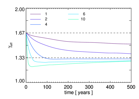
Figure 2.— Evolution of the effective adiabatic index $\gamma_{\mathrm{eff}}$ at the shock front for different values of the injection rate $\eta$ (see legend in units of $10^{-4}$) (derived from Ferrand et al. 2010).

We started the 3D simulations once almost all ($>98$%) the explosion energy is kinetic (in most of our simulations this happens few days after the SN explosion). Then we followed the expansion of the remnant through the RSG wind during the first 340 years of evolution. The initial remnant radius varies between 20 and 200 AU (namely between $10^{-4}$ and $10^{-3}$ pc), depending on the initial radius of the progenitor star. The output of the SN simulations provides the initial radial structure of the ejecta for the SNR simulations.

Several theoretical studies predict that the remnants of core-collapse SNe are characterized by small-scale clumping of material and larger-scale anisotropies (e.g. Li et al. 1993; Wang et al. 2002; Kifonidis et al. 2006; Wang & Wheeler 2008; Gawryszczak et al. 2010, and references therein). Since these structures cannot be described by our 1D SN simulations, we account for them by prescribing an initial clumpy structure of the ejecta and large-scale anisotropies (as suggested by Kifonidis et al. 2006), after the 1D radial density distribution of ejecta (calculated with the SN simulations) is mapped into 3D.

The small-scale ejecta clumps are modeled as per-cell random density perturbations. Following Orlando et al. (2012), we derived these perturbations by adopting a power-law probability distribution with index $\xi=-1$. The parameter characterizing the distribution is the maximum density perturbation that is possible to reach in the simulation. For the purposes of this paper, we assumed that the small-scale clumps have initial size about 2% of the initial remnant radius and a maximum density contrast (namely a density perturbation) $\nu_{\rm max}=5$. These values are in agreement with those suggested by spectropolarimetric studies of SNe (e.g. Wang et al. 2003, 2004; Wang & Wheeler 2008; Hole et al. 2010).

The post-explosion large-scale anisotropies in the ejecta distribution are modeled as overdense spherical knots (hereafter called “shrapnels”) in pressure equilibrium with the surrounding ejecta. Our primary goal is to derive the mass and energy of the anisotropies responsible for the inhomogeneous distribution of Fe and Si/S observed today in Cas A. To this end, we explored the space of parameters characterizing the initial shrapnels to find those best reproducing the observations. In particular, we considered shrapnels initially located either within or outside the iron core, at distance $D_{\rm knot}$ from the center, with radius $r_{\rm knot}$ ranging between 3% and 10% of the initial remnant radius, with density between 10 and 100 times larger than those of the surrounding ejecta at distance $D_{\rm knot}$ (density contrast $\chi_{\rm n}$), and with radial velocity between 1 and 3.5 times larger than that of the surrounding ejecta (velocity contrast $\chi_{\rm v}$). These ranges of values are consistent with those derived from multi-dimensional simulations of core-collapse SNe which show that Rayleigh-Taylor instabilities are seeded by the flow-structures resulting from neutrino-driven convection and are effective at creating metal-rich knots at the terminal ends of Rayleigh-Taylor fingers (e.g. Kifonidis et al. 2003; Ellinger et al. 2012). These knots present dimensions ranging between 2% and 16% of the remnant radius at the time of knot formation and are more than one order of magnitude denser than the surrounding ejecta (e.g. Ellinger et al. 2012). Also the simulations show that the metal fingers and clumps are much faster than the surrounding medium (with velocities up to 5000 km s^-1) and are correlated with the biggest and fastest-rising plumes of neutrino-heated matter (e.g. Wongwathanarat et al. 2015).

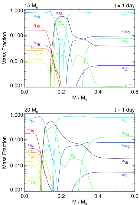
Figure 3.— Isotopic composition of the ejecta as it results from post-shock SN processing of a core-collapse SN originating from a $15\,M_{\rm\odot}$ (upper panel) and $20\,M_{\rm\odot}$ (lower panel) MS star (derived from Thielemann et al. 1996). Only the dominant abundances of intermediate mass nuclei are considered.

As initial isotopic composition of the ejecta, we adopted that derived by Thielemann et al. (1996) for a core-collapse SN either from a $15\,M_{\rm\odot}$ or from a $20\,M_{\rm\odot}$ MS star, namely the extremes of the range of masses suggested in the literature (e.g. Aldering et al. 1994; Lee et al. 2014). Fig. 3 shows the dominant abundances of elements that we follow in details during the evolution. These elements are those that can allow us to compare the distribution of chemical homogeneous regions of ejecta derived from the simulations with those derived from the analysis of observations (e.g. DeLaney et al. 2010; Hwang & Laming 2012; Milisavljevic & Fesen 2013, 2015). The mean atomic mass $\mu$ for the ejecta considers their isotopic composition (Thielemann et al. 1996), whereas $\mu=1.3$ for the RSG wind, assuming cosmic abundances.

As discussed in Sect. 2.1, we assume that the blast wave from the SN explosion propagates through the wind of the progenitor RSG during the whole evolution. The wind is assumed to be spherically symmetric with gas density proportional to $r^{-2}$ (where $r$ is the radial distance from the progenitor). The wind density at $r=2.5$ pc is constrained by X-ray observations of the shocked wind (Lee et al. 2014). Since the shock compression ratio varies with the injection rate, the wind density is different for models with different $\eta$ (see Table 2) in order to obtain the same post-shock density as inferred from the observations.

Table 2Parameters for the Models of Cas A best reproducing the observations

Modela	$\eta$	$n_{\rm w}$	$E_{\rm cr}$
		[cm-3]	[$10^{50}$ erg]
SN-4M-2.3E-0ETA	0	0.9	0
SN-4M-2.3E-1ETA	$1\times 10^{-4}$	0.81	0.94
SN-4M-2.3E-2ETA	$2\times 10^{-4}$	0.62	1.80
SN-4M-2.3E-4ETA	$4\times 10^{-4}$	0.50	2.20
SN-4M-2.3E-6ETA	$6\times 10^{-4}$	0.44	2.28
SN-4M-2.3E-10ETA	$1\times 10^{-3}$	0.42	2.34

^a In all these models, the explosion energy is $E_{\rm SN}=2.3\times 10^{51}$ erg, the ejecta mass is $M_{\rm env}=4M_{\rm\odot}$, and the progenitor pre-SN radius is $R_{0}=350\,R_{\odot}$.

We studied the chemical evolution of the ejecta by adopting the multiple fluids approach present in FLASH (Fryxell et al. 2000). Each fluid is associated to one of the heavy elements shown in Fig. 3 and initialized with the corresponding abundances of elements reported in the figure. In such a way, we followed the evolution of the isotopic composition of the ejecta and mapped the spatial distribution of heavy elements at the present epoch. During the remnant evolution, the different fluids mix together. At any time $t$ the density of a specific element in a fluid cell is given by $\rho_{\rm el}=\rho C_{\rm el}$, where $C_{\rm el}$ is the mass fractions of each element and the index “el” refers to a different element.

The SN explosion is assumed to sit at the origin of the 3D Cartesian coordinate system $(x_{0},y_{0},z_{0})=(0,0,0)$. The computational domain extends 6 pc in the $x$, $y$, and $z$ directions (the current outer radius of the remnant is $\approx 2.5$ pc, assuming a distance of $\approx 3.4$ kpc; Reed et al. 1995). We assume zero-gradient (outflow) conditions at all boundaries.

The SN explosion and subsequent evolution of Cas A involve very different length and time scales, from the relatively small size of the very fast evolving system in the immediate aftermath of the SN explosion (the remnant radius at the beginning of the 3D hydrodynamic simulations is between $10^{-4}$ and $10^{-3}$ pc) to the larger extension of the slowly expanding remnant (the final remnant radius is $\approx 2.5$ pc). This makes rather challenging the 3D modeling of Cas A and we were able to capture the very different scales involved, by exploiting the adaptive mesh refinement capabilities of FLASH. More specifically, we employed 20 nested levels of refinement, with resolution increasing twice at each refinement level. The refinement/derefinement of the mesh is guided by the changes in mass density and temperature and follows the criterion of Löhner (1987). In addition we kept the computational cost approximately constant during the evolution, by adopting an automatic mesh derefinement scheme in the whole spatial domain (Orlando & Drake 2012): we gradually decreased the maximum number of refinement levels from 20 (at the beginning of the simulations) to 6 (at the end) following the expansion of the remnant. The effective spatial resolution reached at the finest level was $\approx 10^{-6}$ pc ($\approx 10^{-2}$ pc) at the beginning (at the end) of the simulations, corresponding to an effective mesh size of $[5\times 10^{6}]^{3}$ ($[512]^{3}$). In such a way, the number of grid zones per radius of the remnant $N_{\rm pt}$ was $>100$ during the whole evolution, with $N_{\rm pt}\approx 100$ at $t=0$ and $N_{\rm pt}>250$ at $t=340$ yr.

3. Results

3.1. The case of a spherically symmetric explosion

As a first step, we explored the parameter space of the SN-SNR model, assuming a 3D spherically symmetric SN explosion. The simulations considered, therefore, include the small-scale clumpy structure of the ejecta but do not consider any large-scale anisotropy (i.e. the shrapnels; see Sect. 2.3). The aim was to derive the best-fit basic parameters of the model (ejecta mass, explosion energy, RSG wind density, and efficiency of CR acceleration) by comparing model results with observations, in view of the study concerning the effects of large-scale anisotropies on the remnant morphology.

Our observing constraints are the radii and velocities of the forward and reverse shocks as observed at current time (reported in Table 1; see also van Veelen et al. 2009). Another constraint is the density of the shocked RSG wind that is inferred to range between 3 and 5 cm^-3 from the analysis of Chandra observations (Lee et al. 2014). Thus we searched for the parameters ($R_{0}$, $E_{\rm SN}$, and $M_{\rm env}$) of the SN model which reproduce altogether the observed density of the shocked wind and the observed radii and velocities of the forward and reverse shocks. Since the non-thermal emission detected in Cas A indicates that effective acceleration of CRs occurs at the shock fronts (e.g. Abdo et al. 2010), we explored also different values of the injection rate $\eta$ (see Sect. 2.3) to account the feedback of CR acceleration on the remnant expansion. Considering that the shock compression ratio increases with $\eta$ (due to a faster decrease of the effective adiabatic index; see Fig. 2), we varied accordingly the pre-shock wind density $n_{\rm w}$ at $r=2.5$ pc (namely the current outer radius of Cas A).

In all the cases explored, the SN-SNR simulations consist of two main phases: the post-explosion evolution of the supernova (lasting few hundreds days since the outburst) and the transition from SN to SNR. The first phase starts when the shock wave following the core-collapse reaches the stellar surface. Then the evolution follows the general trend described by Pumo & Zampieri (2011) and it is briefly summarized below. Initially the envelope is completely ionized and optically thick. Most of the internal energy is gradually released, contributing to the gross emission of the SN. Few days after, the ejecta start to recombine and the shock front recedes through the envelope. In this phase, the resulting sudden release of energy dominates the SN emission. After the envelope is fully recombined and optically thin to optical photons, the SN emission originates from the thermalization of the energy deposited by $\gamma$-ray photons.

The second phase starts few hundreds days after the SN event. We followed the transition from SN to SNR for 340 years. During this time a forward and a reverse shocks are formed, the former propagating into the RSG wind and the latter driven back into the ejecta. The ejecta clumps interact with each other and enhance the development of hydrodynamic instabilities that enhance the mixing of layers with different isotopic composition.

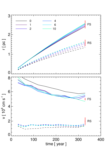
Figure 4.— Angle-averaged radii (upper panel) and velocities (lower panel) of the forward (solid lines) and reverse (dashed lines) shocks vs. time for models assuming a different value of injection rate $\eta$ (see legend in units of $10^{-4}$; see also Fig. 2). The red crosses show the corresponding observational values at the current age of Cas A (see Table 1); the vertical lines of the crosses show the observational uncertainty.

At $t=340$ yr we compared the angle-averaged radii and velocities of the forward and reverse shocks resulting from our models with those observed. Fig. 4 shows these quantities for the models best reproducing the observations together with the observed values at the current epoch. The models in the figure differ from each other for the injection rate $\eta$ and, consequently, for the wind density $n_{\rm w}$ at $r=2.5$ pc (see Table 2). We found that the observations are best reproduced by models characterized by a total ejecta energy $E_{\rm SN}=2.3\times 10^{51}$ erg, an envelope mass $M_{\rm env}=4\,M_{\odot}$ (which has been fixed in our simulations), and a progenitor radius $R_{0}=350\,R_{\odot}$. Our best-fit explosion energy is in good agreement with the value inferred from the observations, $E_{\rm SN}\approx 2\times 10^{51}$ erg (e.g. Laming & Hwang 2003; Hwang & Laming 2003); the ejecta mass is within the range of values discussed in the literature, $M_{\rm ej}=2-4M_{\odot}$ (e.g. Laming & Hwang 2003; Hwang & Laming 2003; Young et al. 2006). We note that our model predicts a total energy which is smaller than that found by Chevalier & Oishi (2003), $E_{\rm SN}\approx 4\times 10^{51}$ erg, on the basis of a 1D hydrodynamic model. Apart from the effects of ejecta clumping that are not included in their model, these authors consider a mass of ejecta, $M_{\rm ej}=3.2\,M_{\odot}$, which is significantly smaller than that adopted here. As a consequence, in their case, a larger total explosion energy is required to fit the observed radius of Cas A. Table 2 summarizes the basic parameters characterizing the SN-SNR models which best-fit our observing constraints: injection rate $\eta$, wind density $n_{\rm w}$ at $r=2.5$ pc, and the fraction of explosion energy converted to CRs $E_{\rm cr}$ at $t=340$ yr; all these models have the same ejecta mass $M_{\rm env}$, explosion energy $E_{\rm SN}$, and progenitor pre-SN radius $R_{0}$.

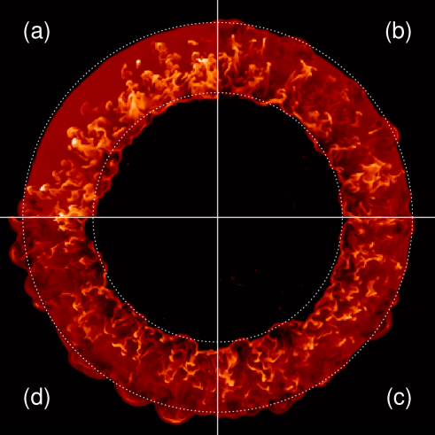
Figure 5.— 2D sections in the $(x,z)$ plane of the spatial density distribution of shocked plasma at $t=340$ yr for runs SN-4M-2.3E-1ETA (a), SN-4M-2.3E-4ETA (b), SN-4M-2.3E-6ETA (c), and SN-4M-2.3E-10ETA (d). The dotted circles mark the observed average position of the forward and reverse shocks in the $(x,z)$ plane.

As expected, the back-reaction of accelerated CRs mainly affects the density structure of the region between the forward and reverse shocks. There the plasma is characterized by an effective adiabatic index $\gamma_{\mathrm{eff}}$ which depends on $\eta$ and varies between $\approx 4/3$ and $5/3$ (see Fig. 2). As a result, the density jump at the shock $\sigma=(\gamma_{\mathrm{eff}}+1)/(\gamma_{\mathrm{eff}}-1)$ varies between 7 and 4. The ejecta clumping enhances the growth of Rayleigh-Taylor instabilities at the contact discontinuity (Orlando et al. 2012). The CR acceleration enhances even further these instabilities. This is shown in Fig. 5 that presents 2D sections in the $(x,z)$ plane of the spatial distribution of plasma density at $t=340$ yr for models with different $\eta$ (runs SN-4M-2.3E-1ETA, SN-4M-2.3E-4ETA, SN-4M-2.3E-6ETA, and SN-4M-2.3E-10ETA). As a consequence of the enhanced intershock Rayleigh-Taylor mixing, the shell of shocked wind is thinner at the forward shock for higher values of $\eta$ and, consequently, the separation between the forward shock and the contact discontinuity is smaller. Panel (c) and, especially, panel (d) of Fig. 5 also show that the enhanced mixing can easily spread the ejecta material close to, or even beyond, the average radius of the forward shock, depending on the size and density contrast of the initial clumps (see also Orlando et al. 2012; Miceli et al. 2013 for more details).

Fig. 4 shows that models differing for the injection rate are all able to fit quite well the radius of the forward shock within the observational uncertainty so that, from the comparison of model results with observations, it is not possible to constrain the value of $\eta$. Nevertheless we note that models with low values of $\eta$ tend to underestimate the radius of the reverse shock and overestimate the velocity of the forward shock. In general our models predict a velocity of the reverse shock which is slightly lower than observed.

For each of the models fitting our observing constraints, we derived the fraction of explosion energy converted to CRs, $E_{\rm cr}$, and compared the simulated values (see Table 2) with those inferred from observations. From the analysis of Fermi data, Abdo et al. (2010) estimated the total content of accelerated CRs as $\approx(1-4)\times 10^{49}$ erg. A similar result has been found by Yuan et al. (2013) who suggest that the total energy lost amounts to $\approx 4\times 10^{49}$ erg. In our model, $E_{\rm cr}$ increases for higher values of $\eta$ and ranges between $9\times 10^{49}$ erg ($\eta=10^{-4}$) and $2.3\times 10^{50}$ erg ($\eta=10^{-3}$), higher than those inferred from the observations. We conclude therefore that the injection rate in Cas A should be slightly lower than $\eta=10^{-4}$.

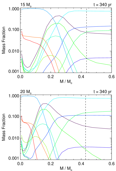
Figure 6.— As in Fig. 3 at $t=340$ yr for run SN-4M-2.3E-1ETA. The dashed lines show the position of the reverse shock.

During the remnant expansion, we followed the evolution of the isotopic composition of ejecta, focusing on the fluids tracing the isotopes of Fe, Si, and S (see Fig. 6), namely those characterizing most of the anisotropies (e.g. jets, pistons) identified in the morphology of Cas A (e.g. DeLaney et al. 2010). We investigated their spatial distribution at $t=340$ yr in the case of a progenitor MS star of either $15M_{\odot}$ or $20M_{\odot}$ and estimated the fraction of their mass which is expected to be shocked. We found that, in average, the stratification of chemical layers at the present age reflects the radial distribution of ejecta in the immediate aftermath of the progenitor SN. It is interesting to note that, from observations, there is evidence that the onion-skin nucleosynthetic layering of the SN has been preserved in some regions of Cas A (Fesen et al. 2006; DeLaney et al. 2010).

On the other hand, in all models of spherically symmetric explosion, the masses of shocked Si and S are significantly lower (by more than 40%) than inferred from observations. More important, we found that no significant amount ($<10^{-3}M_{\odot}$) of shocked Fe is predicted at odds with the results of observations (Hwang & Laming 2012). At first sight, this result may appear to be not surprising, given that the Fe lies deeply in the remnant interior in all our models and the bulk of it has not been reached by the reverse shock at the age of Cas A. However, the ejecta are known to be characterized by a clumpy structure. This may lead to the mixing of initially chemically homogeneous layers and to some overturning of the ejecta due to hydrodynamic instabilities developing during clumps interaction. Our 3D hydrodynamic model shows that the small-scale clumping of ejecta cannot account for the observed redistribution of elements in chemically distinct layers of ejecta in Cas A.

3.2. Effect of a post-explosion anisotropy of ejecta

The results of Sect. 3.1 strongly support the idea that violent dynamical processes have characterized the SN explosion and led to a redistribution of heavy elements in the outer chemical layers. Possible examples of these processes are uneven neutrino heating, axisymmetric magnetorotational effects, hydrodynamic instabilities (e.g. Kifonidis et al. 2003; Wheeler et al. 2002).

Here we investigate how the parameters (size, density, and velocity) of a post-explosion anisotropy formed few hours after the SN event may determine the redistribution of Fe, Si, and S in the outer chemical layers of the remnant. As discussed in Sect. 2.3, the anisotropy is included in the simulations by modeling a large-scale spherical knot (a shrapnel) with given size, density, and velocity. To reduce the computational cost, we performed 3D simulations by considering only one octant of the whole spatial domain (namely the domain extends between 0 and 3 pc in the $x$, $y$, and $z$ directions; see Sect 2.3) and limiting the study to the case of a progenitor MS star of $20\,M_{\odot}$. Reflecting boundary conditions were used at $x=0$, $y=0$, and $z=0$, consistent with the adopted symmetry. Note that analogous simulations have been performed by Miceli et al. (2013) and Tsebrenko & Soker (2015) but in two-dimensions (2D). A major difference with those simulations is that our 3D model describes the post-explosion evolution of the SN and traces the evolution of the isotopic composition of ejecta since few hours after the SN event.

For the basic parameters of the SN-SNR model (mass of ejecta, energy of explosion, injection rate, density of the RSG wind, etc.), we considered those of run SN-4M-2.3E-1ETA (see Table 2) which is one of the models reproducing the main observing constraints of Cas A. We preferred this model to the others because it predicts a fraction of explosion energy converted to CRs that is closer to the values inferred from observations (a factor of $\approx 2$ larger than that suggested by Abdo et al. 2010 and Yuan et al. 2013)

We explored the case of a shrapnel initially located either within the iron core at the distance $D_{\rm knot}=0.15\,R_{\rm SNR}$ from the center (where $R_{\rm SNR}\approx 10$ AU is the initial radius of the remnant 1 day after the SN event) or just outside the iron core at $D_{\rm knot}=0.35\,R_{\rm SNR}$. In all the cases, the shrapnel is placed at an angle of $45^{o}$ with respect to the $x$, $y$, and $z$-axis. The initial radius of the shrapnel is $r_{\rm knot}$, its density and velocity are $\chi_{\rm n}$ and $\chi_{\rm v}$ times larger, respectively, than those of the surrounding ejecta at distance $D_{\rm knot}$ from the center. A summary of the cases explored is given in Table 3.

Table 3Summary of the models describing the evolution of a post-explosion anisotropy of ejecta

Model	$D_{\rm knot}$	$r_{\rm knot}$	$\chi_{\rm n}$	$\chi_{\rm v}$
	[$R_{\rm SNR}$]	[$R_{\rm SNR}$]
Fe-R6-D10-V3.5	0.15	0.06	10	3.5
Fe-R6-D50-V3.5	0.15	0.06	50	3.5
Fe-R6-D100-V3.5	0.15	0.06	100	3.5
Fe-R4-D100-V1.5	0.15	0.04	100	1.5
Fe-R4-D100-V2.5	0.15	0.04	100	2.5
Fe-R4-D100-V3.5	0.15	0.04	100	3.5
Fe-R3-D100-V3.5	0.15	0.03	100	3.5
Si-R10-D10-V1	0.35	0.1	10	1
Si-R10-D5-V3	0.35	0.1	5	3
Si-R10-D3-V5	0.35	0.1	3	5
Si-R10-D1-V10	0.35	0.1	1	10

The evolution of the shrapnel is analogous to that described by Miceli et al. (2013), except for the interaction with the surrounding small-scale clumps of ejecta which are present in our simulations. Initially the shrapnel pushes out through less dense and chemically distinct layers above, favoring the development of hydrodynamic instabilities at its boundary which contribute to its fragmentation. Then the shrapnel enters in the intershock region where it is compressed, heated, and ionized. Also it interacts with Rayleigh-Taylor and Richtmyer-Meshkov instabilities developed at the contact discontinuity. As a result, the shrapnel is partially eroded by the instabilities and evolves towards a core-plume structure. At this stage, its core can be significantly denser than the surrounding shocked ejecta, depending on the initial size and density contrast of the knot.

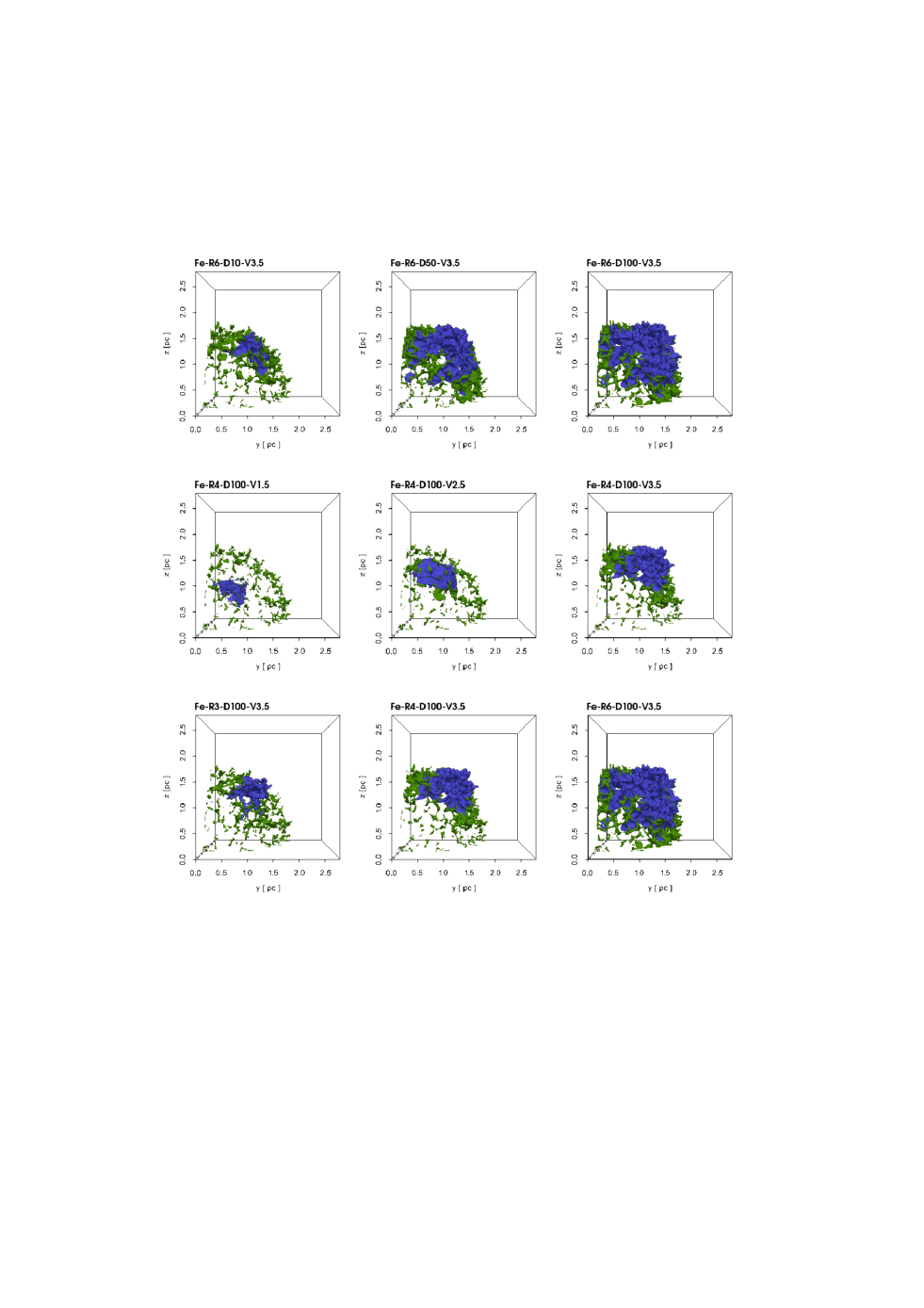
Figure 7.— Spatial distributions of shocked Fe (blue) and Si/S (green) at $t=340$ yr, in the case of a shrapnel initially located within the iron core (see models with $D_{\rm knot}=0.15R_{\rm SNR}$ in Table 3) and assuming a $20M_{\odot}$ progenitor MS star. The figure shows one octant of the domain (the SN explosion occurred at the origin of the 3D Cartesian coordinate system $(x_{0},y_{0},z_{0})=(0,0,0)$) and the colored regions mark material with particle number density $n>0.03$ cm^-3. The upper panels show the distributions for different initial density contrasts $\chi_{\rm n}$, the middle panels for different initial velocity contrasts $\chi_{\rm v}$, and the lower panels for different initial radii of the shrapnel $r_{\rm knot}$.

Fig. 7 shows the spatial distributions of shocked Fe (blue) and Si/S (green) at the age of Cas A, for different parameters of a shrapnel initially located within the iron core ($D_{\rm knot}=0.15\,R_{\rm SNR}$; see Table 3). Depending on its initial density and velocity contrasts, the shrapnel can produce a spatial inversion of ejecta layers, leading to the Si/S-rich ejecta physically interior to the Fe-rich ejecta. A similar effect is observed in Cas A as, for example, in the so-called SE Fe piston: X-ray observations show that Fe-rich ejecta are at a greater radius than Si/S-rich ejecta, and this has been interpreted as an overturning of ejecta layers during the SN explosion (e.g. Hughes et al. 2000). In our simulations, the spatial inversion occurs because the piston is subject to hydrodynamic instabilities which lead to some overturning of the layers in a way analogous that that described by Kifonidis et al. (2006) for the instabilities developed during a SN explosion. The inversion is evident at $t=340$ yr if the initial density contrast of the shrapnel was $\chi_{\rm n}>10$ and its velocity contrast was $\chi_{\rm v}>2.5$ (see upper and middle panels of Fig. 7). Also we found that the presence of the inversion does not depend on the shrapnel size $r_{\rm knot}$, at least in the range of values explored (see lower panel of Fig. 7). This result puts a lower limit to both the density and velocity contrasts of an overdense knot formed in the iron core few hours after the SN explosion in order to produce the spatial inversion of Fe-rich ejecta with Si-rich ejecta observed in Cas A.

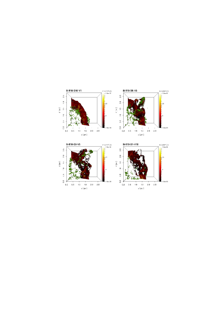
Figure 8.— As in Fig. 7 for a shrapnel initially located outside the iron core (see models with $D_{\rm knot}=0.35R_{\rm SNR}$ in Table 3). In this case, no significant shocked Fe is found. A slice showing the distribution of density, in log scale, in the intershock region is superimposed (see color table on the right of each panel). Each panel shows the result for different combinations of $\chi_{\rm n}$ and $\chi_{\rm v}$.

The final distribution of shocked Si/S in the case of a knot initially located just outside the iron core is shown in Fig. 8. In this case, the simulations showed that knots with $\chi_{\rm v}=1$ do not reach the remnant outline at $t=340$ yr even if their density contrast $\chi_{\rm n}$ is up to 10 (upper left panel in Fig. 8); knots with $\chi_{\rm n}=1$ can perturb the remnant outline at $t=340$ yr if $\chi_{\rm v}=10$ but without producing a collimated Si/S-rich protrusion (see lower right panel in Fig. 8). Indeed a Si/S-rich shrapnel can reach the remnant outline and protrude it, if the initial knot was both denser and faster than the surrounding medium. Knots with initial density and velocity contrasts larger than 1 produce Si-rich jet-like features (see upper right and lower left panels in Fig. 8) which are similar to the NE and SW Si-rich jets observed in Cas A.

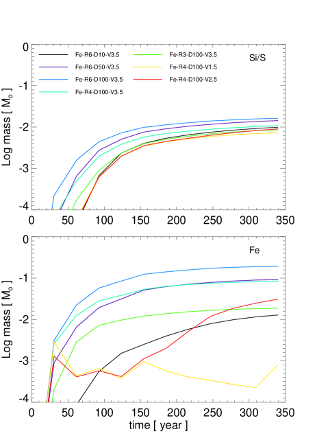
Figure 9.— Amount of shocked Si/S (upper panel) and Fe (lower panel) vs time for models assuming a shrapnel initially located within the iron core ($D_{\rm knot}=0.15R_{\rm SNR}$) and characterized by different parameters (see Table 3).

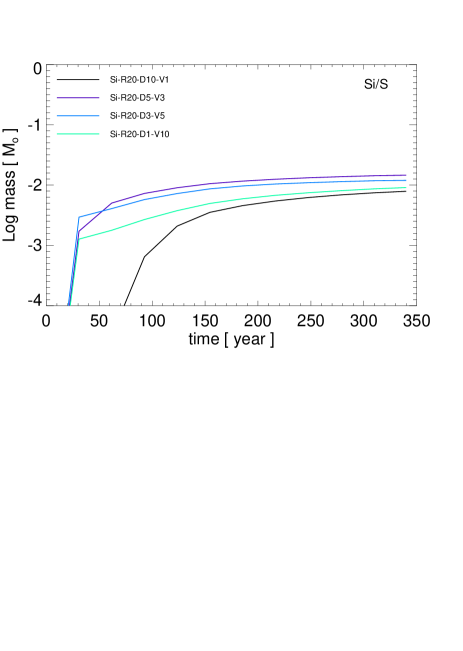
Figure 10.— As in the upper panel of Fig. 9 for models assuming a shrapnel initially located outside the iron core ($D_{\rm knot}=0.35R_{\rm SNR}$; see Table 3).

From the simulations, we derived the amount of shocked Fe and Si/S for the different parameters of the shrapnel (see Figs. 9-10). We found that the amount of shocked Si/S at $t=340$ yr is poorly affected by the initial shrapnel parameters (within the ranges explored) and even by the initial location of the knot (either inside or outside the iron core). The final amount of shocked Si/S ranges between 0.008 and $0.016M_{\odot}$. This is mainly due to the fact that a significant part of the Si/S shell interacts with the reverse shock even without any initial shrapnel, so that the contribution of the latter to the amount of shocked Si/S is poorly relevant. On the other hand, the mass of shocked Fe at $t=340$ yr strongly depends on the initial parameters of the shrapnel. In fact, in the absence of initial anisotropies, the iron core is not reached by the reverse shock during the first 340 yr of evolution (see Sect. 3.1). The shocked Fe observed in the simulations therefore is entirely due to the shrapnel. We found that knots with $\chi_{\rm n}>10$, $\chi_{\rm v}>2.5$, and $r_{\rm knot}>0.03R_{\rm SNR}$ lead up to $\approx 0.1M_{\odot}$ of shocked Fe (see lower panel in Fig. 9). Finally it is worth noting that significant shocked Fe is produced only if the initial anisotropy was located within the iron core.

3.3. Spatial distribution and chemical composition of the Cas A ejecta

Based on the results obtained in Sect. 3.2, we searched for the initial anisotropies that best reproduce the spatial distribution of Fe and Si/S observed today in Cas A (e.g. DeLaney et al. 2010; Hwang & Laming 2012; Milisavljevic & Fesen 2013). As reference model, we considered the case of a progenitor MS star with $15\,M_{\odot}$ and injection rate $\eta=10^{-4}$ (run CAS-15MS-1ETA). The mass of ejecta, energy of explosion, radius of progenitor star, and density of the RSG wind are those of run SN-4M-2.3E-1ETA (see Table 2). Then we explored the space of parameters characterizing the anisotropies, by adopting an iterative process of trial and error to converge on parameters that reproduce the spatial distribution and mass of shocked Fe and Si/S inferred from observations (Hwang & Laming 2012). Table 4 reports our best-fit parameters describing the initial anisotropies.

Table 4Parameters of the post-explosion anisotropies of ejecta describing the final morphology of Cas A

piston/jet	$D_{\rm knot}$	$r_{\rm knot}$	$\chi_{\rm n}$	$\chi_{\rm v}$	$M_{\rm knot}$	$E_{\rm knot}$
	[$R_{\rm SNR}$]	[$R_{\rm SNR}$]			[$M_{\odot}$]	[$10^{49}erg$]
Fe-rich SE	0.15	0.05	100	4.2	0.10	5.0
Fe-rich SW	0.15	0.02	50	4.2	0.0015	0.076
Fe-rich NW	0.15	0.06	50	4.2	0.10	4.8
Si-rich NE	0.35	0.1	5.0	3.0	0.040	4.2
Si-rich SW	0.35	0.1	1.2	3.0	0.0091	1.0

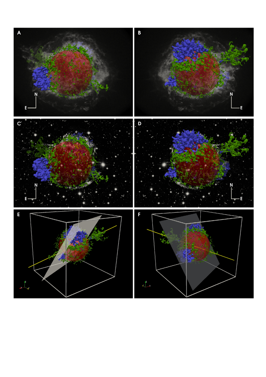
Figure 11.— 3D spatial distribution of Cas A shocked Fe (blue) and Si/S (green) derived from run CAS-15MS-1ETA (see Table 5). Panels A and C show the 3D distribution assuming the vantage point at Earth (the perspective is in the plane of the sky); panels B and D show the same perspective but with the vantage point from behind Cas A (namely the perspective is rotated by $180^{o}$ about the northsouth axis); panels E and F show the distribution from arbitrary points of view. The transparent image in the upper panels (A and B) is a Chandra observation showing the hot shocked plasma in the wavelength band $[0.3,10]$ keV (retrieved from www.nasa.gov); the transparent image in the middle panels (C and D) is a composite Hubble Space Telescope (HST) image sensitive to emission in cold O and S lines (retrieved from www.spacetelescope.org). The transparent red sphere marks the fiducial reverse shock; the transparent plane in panels E and F represents the plane where the initial Fe-rich anisotropies lie; the yellow line in panels E and F shows the direction of propagation of the Si-rich jet and counterjet. Refer to Movie 1 for an animation of these data.

Three of them are located within the iron core at $D_{\rm knot}=0.15\,R_{\rm SNR}$, roughly lying in a plane oriented with an $\approx-30^{o}$ rotation about the $x$-axis (namely the eastwest axis in the plane of the sky) and an $\approx 25^{o}$ rotation about the $z$-axis (the northsouth axis in the plane of the sky; see Fig. 11). The other two are located just outside the iron core at $D_{\rm knot}=0.35\,R_{\rm SNR}$ on a line oriented with an $\approx-67^{o}$ rotation about the $x$-axis and an $\approx 67^{o}$ rotation about the $z$-axis (see Fig. 11). The first three knots reproduce the Fe-rich regions and the others the Si-rich NE jet and SW counterjet observed today in Cas A. Table 4 reports also the masses and energies of the pistons responsible for the observed distribution of Fe and Si/S. We note that the total kinetic energy of all the pistons is about $1.5\times 10^{50}$ erg. Thus the pistons/jets represent a relatively small fraction ($\approx 7$%) of the remnant’s energy budget, at odds with previous estimates (e.g. Willingale et al. 2003; Laming et al. 2006).

We performed additional simulations to explore also the case of a progenitor MS star with $20\,M_{\odot}$ (run CAS-20MS-1ETA) and the case in which there is no feedback of accelerated CRs ($\eta=0$; run CAS-15MS-0ETA). However, from the analysis of the distribution of Si, S, and Fe, we did not find any appreciable difference of these cases with our reference model (run CAS-15MS-1ETA). In the following, therefore, we discuss in detail only the results of run CAS-15MS-1ETA, mentioning the differences (if any) with the other two cases.

3.3.1 Shocked ejecta

Table 5Element Masses Derived from Models and Comparison with Chandra Observations (Hwang & Laming 2012)

Model	Element	$M_{\rm el,sh}/M_{\odot}$	$M_{\rm el,sh}/M_{\rm ej}$
CAS-15MS-1ETA	Si/S	0.076	0.019
	Fe	0.19	0.048
	$M_{\rm ej,sh}$	3.66	0.92
	$M_{\rm ej}$	4	1
CAS-15MS-0ETA	Si/S	0.080	0.020
	Fe	0.19	0.048
	$M_{\rm ej,sh}$	3.70	0.92
	$M_{\rm ej}$	4	1
CAS-20MS-1ETA	Si/S	0.080	0.020
	Fe	0.18	0.045
	$M_{\rm ej,sh}$	3.66	0.92
	$M_{\rm ej}$	4	1
Observationsa	Si/S	0.08	0.03
	Fe	0.14	0.04
	$M_{\rm ej,sh}$	2.84	0.90
	$M_{\rm ej}$	3.14	1

In our favored model, the initial ejecta distribution (at day $\approx 1$ since the SN event) is characterized by five large-scale spherical knots (in addition to the smaller-scale clumpy structure). From our model, we derived the total mass of shocked ejecta at $t=340$ yr, $M_{\rm ej,sh}\approx 3.66\,M_{\odot}$ (see Table 5). This value is larger than that inferred by Hwang & Laming (2012) from the analysis of Chandra observations of Cas A, namely $M_{\rm ej,sh}\approx 2.84\,M_{\odot}$. The latter estimate, however, has been derived by matching the Cas A observations with 1D hydrodynamic models of SNR evolution. We note that their best-fit model considers a total ejecta mass, $M_{\rm ej}\approx 3.14M_{\odot}$, lower than that adopted in our simulations ($M_{\rm ej}\approx 4M_{\odot}$). Indeed, considering the fraction of the total ejecta mass that is shocked at $t=340$ yr, $M_{\rm ej,sh}/M_{\rm ej}$, we found that the value predicted with our model ($\approx 92$ %) is in agreement with that derived by Hwang & Laming (2012) ($\approx 90$ %).

Fig. 11 shows the 3D spatial distribution of shocked Fe and Si/S derived from run CAS-15MS-1ETA, considering different points of view. An on-line animation has been provided that shows the 3D distribution rotated completely about the northsouth axis (Movie 1). The ejecta morphology is dominated by the three Fe-rich regions caused by the initial anisotropies located in the iron core (see Table 4). We note that the SE Fe-rich region has more a jet-like structure if compared with the other regions in agreement with the observations (DeLaney et al. 2010). This is due to the higher density contrast of the corresponding initial anisotropy (see Table 4). As expected on the base of the results of Sect. 3.2, the initial anisotropies produce a spatial inversion of ejecta layers at the age of Cas A, leading locally to Fe-rich ejecta placed at a greater radius than Si/S-rich ejecta.

A striking aspect is that the Fe-rich regions are circled by rings of Si/S-rich ejecta. In particular we can identify clearly two complete rings around the NW and SE Fe-rich regions (see Movie 1). These features resemble the cellular structure of [Ar II], [Ne II], and Si XIII observed in Cas A that appears as rings on the surface of a sphere (e.g. DeLaney et al. 2010). The Si/S-rich rings form as a result of the high velocity Fe-rich ejecta pistons (the shrapnels) in a way similar to that suggested by DeLaney et al. (2010). Each piston pushes out the chemically distinct layers above and, at some point, it breaks through some of them, leading to the spatial inversion of ejecta layers (see Sect. 3.2). Then the material of the outer layers (in particular the Si/S) is swept out by the piston and progressively accumulates at its sides. As a result, when the piston encounters the reverse shock, a region of shock-heated Fe forms which is enclosed by a ring of shock-heated Si/S.

The post-explosion anisotropies located just outside the iron core are responsible for the Si/S-rich jets (see Fig. 11 and Movie 1). In this case the shrapnels (given the initial values of their density and velocity contrasts) break through the outer ejecta layers, thus not preserving locally the original onion-skin nucleosynthetic layering. Then the shrapnels are able to protrude the remnant outline, thus forming wide-angle ($\approx 40^{o}$) opposing streams of Si/S-rich ejecta in the NE and SW quadrants. This is consistent with the scenario proposed to explain the origin of the Si/S-rich NE jet and SW counterjet observed in Cas A (e.g. Fesen et al. 2006). The streams travel at velocities up to $\approx 10000$ km s^-1 in agreement with the values inferred from the observations (Fesen 2001; Hwang et al. 2004; Fesen & Milisavljevic 2015).

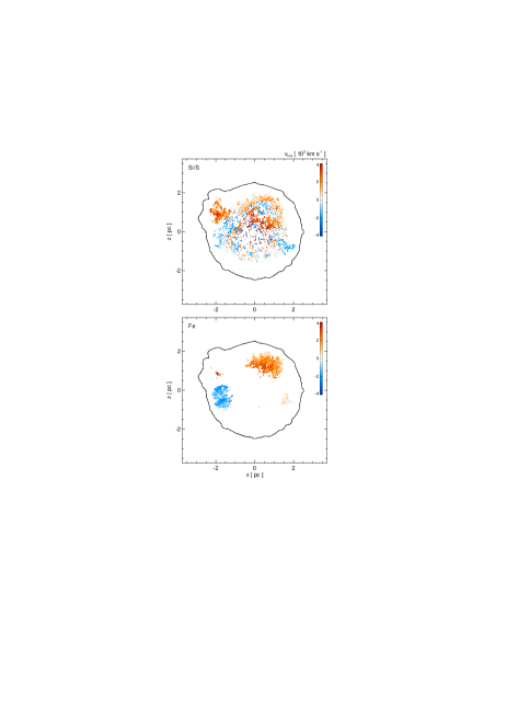
Figure 12.— 2D maps of average emission-measure-weighted velocity along the line-of-sight, $v_{los}$, for shocked Si/S (upper panel) and Fe (lower panel) derived from run CAS-15MS-1ETA. The approximate velocity range is $\pm 4000$ km s^-1 (see color bar on the right in units of $10^{3}$ km s^-1). These images correspond to effective Doppler maps derived from observations.

The pistons correspond to regions where relatively faster-moving ejecta were expelled. Fig. 12 shows the average emission-measure-weighted velocity of shocked Fe and Si/S along the line of sight derived from our model. The shocked Si/S is mostly concentrated in the redshifted jet to the NE and a large redshifted ring-like feature to the NW. The latter is the result of the piston which breaks through the Si/S layer and is responsible for the large Fe-rich region to the NW. These two features are those with the highest absolute values of velocity along the line of sight, $\approx 4000$ km s^-1. In the case of the NE jet (inclined with an angle of $23^{o}$ with respect to the plane of the sky), this corresponds to the high velocity values of the streams of $\approx 10000$ km s^-1 derived from the simulation. The SW jet and the SE piston are visible as blueshifted material. The shocked Fe is concentrated in the most prominent redshifted area to the NW and the blueshifted area to the SE. We note that the velocity pattern of shocked Fe is remarkably similar to the Doppler images derived from observations of Cas A (e.g. Willingale et al. 2002; DeLaney et al. 2010). In particular it matches the approximate velocity range inferred from observations, namely $\pm 4000$ km s^-1.

From the models we calculated the masses of Fe and Si/S in shocked ejecta at $t=340$ yr (see Table 5) and compared them with the values inferred from the analysis of Chandra observations (Hwang & Laming 2012). We found that the models adopting the parameters of the anisotropies summarized in Table 4 reproduce quite well the mass of shocked Fe. On the other hand, all our models slightly underestimate the fraction of mass of shocked Si/S, $M_{\rm Si/S,sh}/M_{\rm ej}$, by $\approx 30$% (see Table 4). This was somehow expected on the basis of the results of Sect. 3.2. In fact, the effect of the initial asymmetries is only to slightly increase the mass of shocked Si/S with respect to the case of a spherically symmetric explosion. Thus a way to increase significantly the mass of shocked Si/S might be to change the initial isotopic composition adopted for the ejecta. However, we found that our result does not change either if we adopt a progenitor MS star with $20\,M_{\odot}$ (run CAS-20MS-1ETA in Table 5) or if we neglect the effects of CRs acceleration (run CAS-15MS-0ETA). Nevertheless we note that our models as well as the values inferred from the observations are subject to some uncertainties, so that a discrepancy of the order of 30% may be considered satisfactory.

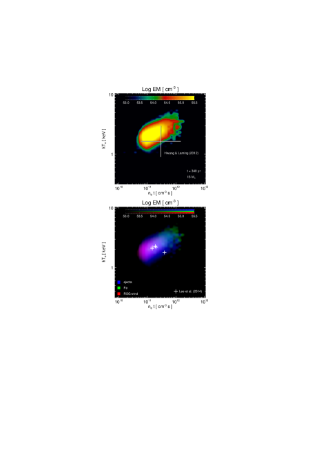
Figure 13.— Upper panel: distribution of emission measure vs. electron temperature $kT_{\rm e}$ and ionization age $n_{\rm e}t$ at $t=340$ yr derived from run CAS-15MS-1ETA. The white cross shows the ranges of $kT_{\rm e}$ and $n_{\rm e}t$ values inferred from Chandra observations (Hwang & Laming 2012). Lower panel: corresponding three-color composite image of the emission measure distribution. The colors show the contribution to emission measure from the shocked ejecta (blue), shocked Fe (green), and shocked RSG wind (red). The white crosses mark the values derived by Lee et al. (2014) from the analysis of regions dominated by thermal emission of shocked ambient gas.

Fig. 13 shows the emission measure distribution as a function of electron temperature, $kT_{\rm e}$, and ionization age, $n_{\rm e}t$, for the shocked plasma at the age of Cas A. The X-ray emitting plasma is largely out of equilibrium of ionization with the emission measure distribution peaking at $kT_{\rm e}\approx 2$ keV and $n_{\rm e}t\approx 10^{11}$ cm^-3 s in a region dominated by shocked ISM (see upper panel in Fig. 13). These values are in excellent agreement with the best-fit parameters derived by Lee et al. (2014) from the analysis of X-ray spectra extracted from several regions around the outermost boundary dominated by thermal emission of shocked ambient gas (see lower panel in Fig. 13). A more complete comparison of our model results with observations is obtained by considering the analysis of Chandra observations of Hwang & Laming (2012). These authors provided a consistent spectral characterization of the entire remnant of Cas A by defining a grid of macropixels across the remnant and analyzing every spectrum in the grid. In such a way, they were able to derive the distributions of ionization ages and electron temperatures of the entire remnant. We found that our simulation predicts $kT_{\rm e}$ and $n_{\rm e}t$ values in the observed ranges. The distributions of $kT_{\rm e}$ and $n_{\rm e}t$ derived from the simulation are highly peaked in agreement with the findings of Hwang & Laming (2012) who suggested that the peaked distributions result from the multiple secondary shocks following reverse shock interaction with ejecta inhomogeneities. Fig. 13 shows also that the shocked Fe is at an advanced ionization age ($n_{\rm e}t\approx 10^{12}$ cm^-3 s) relative to the other elements. This is also in nice agreement with the observations (e.g. Hwang & Laming 2003, 2012).

3.3.2 Unshocked ejecta

In our model, the total mass of unshocked ejecta at the age of Cas A is $\approx 0.34\,M_{\odot}$. This value is in good agreement with that inferred from the analysis of low frequency ($<100$ MHz) radio observations ($\approx 0.39\,M_{\odot}$; DeLaney et al. 2014) and that derived by Hwang & Laming (2012) by interpreting the Chandra observations with hydrodynamic models ($\approx 0.30\,M_{\odot}$).

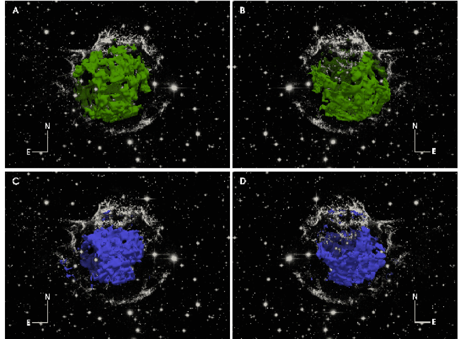
Figure 14.— 3D spatial distribution of Cas A unshocked Si/S (green, upper panels) and Fe (blue, lower panels) derived from run CAS-15MS-1ETA. Panels A and C show the 3D distribution assuming the vantage point at Earth; panels B and D show the same perspective but with the vantage point from behind Cas A. As in Fig.11, the transparent image in the panels is a composite HST image. Refer to Movie 2 for an animation of these data.

The 3D spatial distributions of unshocked Fe and Si/S are reported in Fig. 14. An on-line animation shows the 3D distribution rotated completely about the northsouth axis (Movie 2). The majority of the unshocked Si/S follows roughly the original onion-skin nucleosynthetic layering. However, the original Si/S layer is characterized by five large cavities corresponding to the directions of propagation of the post-explosion anisotropies (pistons/jets). The regions of shocked Fe observed in the main-shell and the NE and SW jets are located exactly above the cavities. We also found that the cavities are physically connected to some of the rings of shocked Si/S in the main-shell as, for instance, in the case of the NW and SE cavities (compare Figs. 11 and 14, and Movies 1 and 2). The average structure of the unshocked Si/S is somehow reminiscent of the bubble-like morphology characterizing the remnant interior of Cas A, inferred from the analysis of near-infrared spectra of the remnant including the [S III] 906.9 and 953.1 nm (Milisavljevic & Fesen 2015).

The Fe-rich NW and SE pistons are responsible for the largest cavities in our simulations, with the NW cavity with a radius of $\approx 0.88$ pc and the SE cavity with a radius of $\approx 0.54$ pc. These values are also in good agreement with those estimated from the analysis of observations (Milisavljevic & Fesen 2015). On the other hand, the distribution of unshocked S derived from the analysis of near-infrared spectra appears much more structured than in our simulations. This may suggest that a number of smaller-scale pistons with lower velocity and/or density contrast (not considered in our simulations) might be present in Cas A.

The structure of Si/S is filled by unshocked Fe (see Fig. 14 and Movie 2) with a density below 0.1 cm^-3. Most of the Fe is concentrated in the remnant core and shows a clumpy structure in agreement with the expectation of strong instabilities associated with the explosion reverse shock during the first few hours after the SN explosion. The distribution of Fe is roughly spherically symmetric, although large cavities are evident which correspond to the regions of the initial pistons. The total mass of unshocked Fe derived from the model is $\approx 0.1\,M_{\odot}$.

Our model predicts a low-density and low-temperature environment in the unshocked ejecta. The average density derived from the simulation is $\rho\approx 2\times 10^{-24}$ g cm^-3. From the analysis of radio observations of Cas A, DeLaney et al. (2014) derive a density $\rho\approx 5.5\times 10^{-24}$ g cm^-3, assuming a uniform density ejecta distribution throughout the remnant interior with no clumping. The hydrodynamic models considered by Hwang & Laming (2012) to interpret the Chandra observations of Cas A predict a density $\rho\approx 1\times 10^{-24}$ g cm^-3 at an age of 330 yr. The temperature of the unshocked ejecta is rather low due to the rapid expansion of the SNR and ranges between $\approx 10$ K (close to the origin of the SN explosion) and $\approx 10^{3}$ K (immediately before the reverse shock). These temperatures are consistent with the analysis of the Spitzer infrared data (e.g. Eriksen et al. 2009) and with the evidence that unshocked dust temperatures of about 35 K are observed in the infrared band (e.g. Nozawa et al. 2010).

4. Summary and conclusions

We studied the evolution of ejecta in the SNR Cas A with the aim to investigate the origin of the asymmetries observed today in its morphology. In particular, we investigated the scenario of high velocity pistons of ejecta emerging from the SN explosion proposed by DeLaney et al. (2010) to explain the distribution of Fe-rich regions and Si-rich jets observed today in Cas A. To this end, we developed a hydrodynamic model describing the evolution of Cas A from the immediate aftermath of the SN explosion to the remnant expansion through the wind of the progenitor RSG, thus covering the evolution of the system from few seconds after the SN event till the current age of the remnant ($t=340$ yr). The model includes the effects on shock dynamics due to back-reaction of accelerated cosmic rays and describes the initial structure of the ejecta through small-scale clumping of material and larger-scale anisotropies, according to indications from theoretical studies (e.g. Li et al. 1993; Wang et al. 2002; Kifonidis et al. 2006; Wang & Wheeler 2008; Gawryszczak et al. 2010, and references therein). The model follows the evolution of the post-explosion isotopic composition of the ejecta in order to trace the distribution of Si, S, and Fe, namely the elements characterizing most of the anisotropies (e.g. jets, pistons) identified in the morphology of Cas A (e.g. DeLaney et al. 2010; Milisavljevic & Fesen 2013).

We explored the parameter space of the model searching for the values of ejecta mass, $M_{\rm ej}$, and explosion energy, $E_{\rm SN}$, best reproducing the radii and velocities of the forward and reverse shocks as observed at the current time ($t=340$ yr), and the density of the shocked RSG wind inferred from observations. The best match was found for models with $M_{\rm ej}\approx 4M_{\odot}$ and $E_{\rm SN}\approx 2.3\times 10^{51}$ erg. These values are in good agreement with those estimated from the analysis of observations (Laming & Hwang 2003; Hwang & Laming 2003; Young et al. 2006). It is worth noting that, in our simulations, the envelope mass, $M_{\rm ej}$, was fixed equal to $4M_{\odot}$ (according to Young et al. 2006 and van Veelen et al. 2009) in order to reduce the computational cost in the exploration of the parameter space. On the other hand, an envelope mass of $\approx 3-5\,M_{\odot}$ would not considerably deviate from the observations. We expect that, adopting lower values of $M_{\rm ej}$, the explosion energy $E_{\rm SN}$ required to fit our observational constraints would be larger than that found here. The opposite is expected for higher values of $M_{\rm ej}$. On the other hand, the explosion energy that we found for $M_{\rm ej}\approx 4M_{\odot}$ is very close to that inferred from the observations ($\approx 2\times 10^{51}$ erg; Laming & Hwang 2003; Hwang & Laming 2003), so that we are confident that the envelope mass adopted here is not far away from the true value. Our best-fit models also predict that the radius of the progenitor RSG at the explosion was $R_{0}\approx 300-400\,R_{\odot}$. It is interesting to note that this value is compatible with a RSG that has lost a significant fraction of its H-rich envelope before the SN event (e.g. Bersten et al. 2012).

The evidence of non-thermal emission in Cas A suggests that effective acceleration of CRs occurs at the shock fronts. Thus we investigated the effects of back-reaction of accelerated CRs on the shock dynamics for different injection rates $\eta$. We found that the fraction of explosion energy converted to CRs at the current epoch increases with $\eta$ and ranges between $\approx 9\times 10^{49}$ erg ($\eta=10^{-4}$) and $\approx 2.3\times 10^{50}$ erg ($\eta=10^{-3}$). These values are larger than those inferred from the observations (namely $\approx 4\times 10^{49}$ erg; Abdo et al. 2010; Yuan et al. 2013), suggesting that the injection rate in Cas A is $\eta<10^{-4}$. Since the plasma compressibility increases in the presence of CR acceleration, a less dense RSG wind is needed to fit the observed radii and velocities of the forward and reverse shocks. In the case of a very efficient CR acceleration ($\eta=10^{-3}$), our model predicts a wind density $n_{\rm w}\sim 0.4$ cm^-3 at $r\approx 2.5$ pc, suggesting that the swept-up mass of the RSG wind is $M_{\rm w,sh}\approx 3M_{\odot}$ (see Eq. 1). Note that the value $M_{\rm w,sh}\approx 6M_{\odot}$ derived in Sect. 2.1 for negligible CR acceleration is an upper limit to the shocked mass of the wind.

It is interesting to note that models with different $\eta$ required the same explosion energy to fit our observational constraints, despite the amount of energy lost in CRs acceleration is larger for higher values of $\eta$. This is explained because a lower density of the RSG wind was required to fit the observed density of the shocked wind. In fact, on one hand, the energy lost produces a slowdown and, on the other hand, the lower wind density produces a speedup of the forward shock. We found that the two effects cancel out each other in our simulations, so that the same explosion energy is required for different values of $\eta$.

We investigated the effects that high-velocity pistons emerging from the SN explosion have on the final remnant morphology. In particular, we explored the parameter space of the initial pistons with the aim to reproduce the spatial distribution and the masses of shocked Fe and Si/S inferred from the observations of Cas A. For this exploration, we considered the initial size of the shrapnels and their contrasts of density and velocity with respect to the surrounding ejecta. Since the physical quantities characterizing the shrapnels are set relatively to the surrounding medium, we do not expect significant changes in our results if different total mass of ejecta (which affects their density) and/or explosion energy (affecting the density and velocity of ejecta) were adopted in the simulations. In all the cases explored we found that the initial shrapnels are gradually fragmented into smaller clumps as the remnant evolves. In particular this happens when the shrapnels are compressed and heated by the reverse shock arising from the interaction of the remnant with the RSG wind.

The model best matching the observations predicts that, at least, five large-scale anisotropies have developed in the immediate aftermath of the SN explosion. Three of them were located within the iron core and reproduce the Fe-rich regions observed today in Cas A. The other two were located just outside the iron core and reproduce the Si-rich NE jet and SW counterjet. The parameters characterizing these anisotropies (namely their initial size, and the velocity and density contrasts) are consistent with those found through multi-dimensional modeling of SN explosions for the dense knots produced by Rayleigh-Taylor instabilities seeded by flow structures resulting from neutrino-driven convection (e.g. Kifonidis et al. 2003; Ellinger et al. 2012). We determined the energies and masses of the initial anisotropies and found that they had a total mass of $\approx 0.25\,M_{\odot}$ and a total kinetic energy of $\approx 1.5\times 10^{50}$ erg, thus representing a small fraction of the total ejecta mass ($\approx 5$%) and of the remnant’s energy budget ($\approx 7$%).

We note that our simulations predict that the initial pistons were faster than the surrounding ejecta. Interestingly, Wongwathanarat et al. (2015), through 3D modeling of core-collapse SNe, have found that SN explosions from RSG progenitors with $15\,M_{\odot}$ (at variance with SNe from blue supergiant progenitors) present a large development of fast plumes of Ni-rich ejecta which grow into extended fingers from which fast metal-rich clumps detach. This leads to a global metal asymmetry characterized by pronounced clumpiness, and a deep penetration of Ni fingers into the overlying layers of ejecta.

In regions not affected by large-scale anisotropies, the average chemical stratification of the ejecta few days after the SN event is roughly maintained in the subsequent evolution until the current age of Cas A. Thus, although the rapid ejecta expansion is certainly not homologous because clumps and instabilities may easily develop (e.g. Wang & Chevalier 2001; Orlando et al. 2012), our model suggests that the abundance pattern observed in young SNRs keeps memory of the radial distribution of heavy elements in the aftermath of the explosion in regions not affected by the large-scale anisotropies developed during the SN event. This result explains the evidence that, apparently, the onion-skin nucleosynthetic layering of the SN has been preserved in some regions of Cas A (e.g. Fesen et al. 2006; DeLaney et al. 2010), namely those not affected by the initial pistons.

On the other hand, the chemical stratification is not preserved in regions strongly affected by the pistons/jets propagation. The pistons responsible for Si/S-rich jets break through the outer ejecta layers, protruding the remnant outline and forming opposing streams of Si/S-rich ejecta in the NE and SW quadrants. The Fe-rich pistons produce a spatial inversion of ejecta layers, leading to the Si/S-rich ejecta physically interior to the Fe-rich ejecta. In fact, each piston is subject to hydrodynamic instabilities during its propagation and this lead to some overturning of the chemical layers. Again, this result matches nicely with the evidence that Fe-rich ejecta are at a greater radius than Si/S-rich ejecta in the Fe-rich regions of shocked ejecta observed in Cas A (e.g. Hughes et al. 2000).

A striking feature is that the regions of Fe-rich shocked ejecta are circled by rings of Si/S-rich shocked ejecta. These rings are the result of the dynamics of high-velocity pistons emerging from the SN explosion. As a snowplow, each piston pushes the layers above to the side, causing a progressive accumulation of chemically distinct material (in particular Si/S) around the piston itself. As a result, when the piston encounters the reverse shock, a central region of shocked Fe circled by a ring enriched of shocked Si/S forms. An example is the region of Fe-rich shocked ejecta to the NW (see Fig. 11 and Movie 1).

The modeled rings are consistent with the bright rings of [Ar II], [Ne II], and Si XIII around the Fe-rich regions observed in Cas A (e.g. Morse et al. 2004; Patnaude & Fesen 2007; DeLaney et al. 2010). Thus our model provides evidence that high-velocity pistons emerging from the SN explosion may explain the origin of the bright rings observed in Cas A, supporting the original scenario proposed by DeLaney et al. (2010). We note however that the observed rings are much more pronounced than those in our simulations. A role might be played by the magnetic field which is neglected in our model. If the ejecta are magnetized, the clumps are expected to be preserved and longer-living because the field would envelope the ejecta clumps, limiting the growth of hydrodynamic instabilities contributing to their fragmentation (e.g. Orlando et al. 2012). As a result, the clumps of chemically distinct material pushed to the side of the pistons might survive for a longer time, producing more evident and brighter rings.

A further support to the scenario of high-velocity pistons comes from the analysis of the deviations from equilibrium of ionization of shocked plasma. Our simulations predict that the shocked Fe is at an advanced ionization age ($n_{\rm e}t\approx 10^{12}$ cm^-3 s) relative to the other elements, in excellent agreement with Chandra observations of Cas A (e.g. Hwang & Laming 2012). It is interesting to note that the evidence of an advanced ionization age of shocked Fe is considered as an argument against the origin of Fe-rich regions from expanding plumes of radioactive ⁵⁶Ni-rich ejecta which predicts much lower ionization ages (e.g. Li et al. 1993; Blondin et al. 2001; Milisavljevic & Fesen 2015).

Finally we analyzed also the distribution of unshocked ejecta and found that our model reproduces the main features observed in the radio and near-infrared bands. The distribution of unshocked Si/S is characterized by large cavities corresponding to the directions of propagation of the pistons/jets. This explains why the cavities observed in near-infrared observations are physically connected to the bright rings in the main-shell (e.g. Milisavljevic & Fesen 2015). Our model predicts that the structure of Si/S is filled by low-density unshocked Fe. We estimated a total mass of unshocked Fe of $\approx 0.1\,M_{\odot}$.

References

- Abdo et al. (2010) Abdo, A. A. et al. 2010, ApJ, 710, L92
- Aldering et al. (1994) Aldering, G., Humphreys, R. M., & Richmond, M. 1994, AJ, 107, 662
- Badenes et al. (2008) Badenes, C., Hughes, J. P., Cassam-Chenaï, G., & Bravo, E. 2008, ApJ, 680, 1149
- Bersten et al. (2012) Bersten, M. C. et al. 2012, ApJ, 757, 31
- Blasi (2002) Blasi, P. 2002, Astroparticle Physics, 16, 429
- Blasi (2004) —. 2004, Astroparticle Physics, 21, 45
- Blondin et al. (2001) Blondin, J. M., Borkowski, K. J., & Reynolds, S. P. 2001, ApJ, 557, 782
- Chevalier & Oishi (2003) Chevalier, R. A., & Oishi, J. 2003, ApJ, 593, L23
- Colella & Woodward (1984) Colella, P., & Woodward, P. 1984, JCP, 54, 174
- Crowther (2007) Crowther, P. A. 2007, ARA&A, 45, 177
- Dall’Ora et al. (2014) Dall’Ora, M. et al. 2014, ApJ, 787, 139
- DeLaney et al. (2014) DeLaney, T., Kassim, N. E., Rudnick, L., & Perley, R. A. 2014, ApJ, 785, 7
- DeLaney et al. (2004) DeLaney, T., Rudnick, L., Fesen, R. A., Jones, T. W., Petre, R., & Morse, J. A. 2004, ApJ, 613, 343
- DeLaney et al. (2010) DeLaney, T. et al. 2010, ApJ, 725, 2038
- Dwarkadas (2014) Dwarkadas, V. V. 2014, MNRAS, 440, 1917
- Dwarkadas et al. (2010) Dwarkadas, V. V., Dewey, D., & Bauer, F. 2010, MNRAS, 407, 812
- Ellinger et al. (2012) Ellinger, C. I., Young, P. A., Fryer, C. L., & Rockefeller, G. 2012, ApJ, 755, 160
- Eriksen et al. (2009) Eriksen, K. A., Arnett, D., McCarthy, D. W., & Young, P. 2009, ApJ, 697, 29
- Ferrand et al. (2010) Ferrand, G., Decourchelle, A., Ballet, J., Teyssier, R., & Fraschetti, F. 2010, A&A, 509, L10
- Fesen (2001) Fesen, R. A. 2001, ApJS, 133, 161
- Fesen et al. (2006) Fesen, R. A. et al. 2006, ApJ, 645, 283
- Fesen & Milisavljevic (2015) Fesen, R. A., & Milisavljevic, D. 2015, ArXiv e-prints
- Fryxell et al. (2000) Fryxell, B. et al. 2000, ApJS, 131, 273
- Garcia-Segura et al. (1996) Garcia-Segura, G., Langer, N., & Mac Low, M.-M. 1996, A&A, 316, 133
- Gawryszczak et al. (2010) Gawryszczak, A., Guzman, J., Plewa, T., & Kifonidis, K. 2010, A&A, 521, A38
- Ghavamian et al. (2007) Ghavamian, P., Laming, J. M., & Rakowski, C. E. 2007, ApJ, 654, L69
- Gotthelf et al. (2001) Gotthelf, E. V., Koralesky, B., Rudnick, L., Jones, T. W., Hwang, U., & Petre, R. 2001, ApJ, 552, L39
- Hole et al. (2010) Hole, K. T., Kasen, D., & Nordsieck, K. H. 2010, ApJ, 720, 1500
- Hughes et al. (2000) Hughes, J. P., Rakowski, C. E., Burrows, D. N., & Slane, P. O. 2000, ApJ, 528, L109
- Hwang & Laming (2003) Hwang, U., & Laming, J. M. 2003, ApJ, 597, 362
- Hwang & Laming (2009) —. 2009, ApJ, 703, 883
- Hwang & Laming (2012) —. 2012, ApJ, 746, 130
- Hwang et al. (2004) Hwang, U. et al. 2004, ApJ, 615, L117
- Kaastra & Mewe (2000) Kaastra, J. S., & Mewe, R. 2000, in Atomic Data Needs for X-ray Astronomy, p. 161
- Kifonidis et al. (2003) Kifonidis, K., Plewa, T., Janka, H.-T., & Müller, E. 2003, A&A, 408, 621
- Kifonidis et al. (2006) Kifonidis, K., Plewa, T., Scheck, L., Janka, H.-T., & Müller, E. 2006, A&A, 453, 661
- Kochanek et al. (2012) Kochanek, C. S., Khan, R., & Dai, X. 2012, ApJ, 759, 20
- Krause et al. (2008) Krause, O., Birkmann, S. M., Usuda, T., Hattori, T., Goto, M., Rieke, G. H., & Misselt, K. A. 2008, Science, 320, 1195
- Laming & Hwang (2003) Laming, J. M., & Hwang, U. 2003, ApJ, 597, 347
- Laming et al. (2006) Laming, J. M., Hwang, U., Radics, B., Lekli, G., & Takács, E. 2006, ApJ, 644, 260
- Lee et al. (2014) Lee, J.-J., Park, S., Hughes, J. P., & Slane, P. O. 2014, ApJ, 789, 7
- Levesque et al. (2005) Levesque, E. M., Massey, P., Olsen, K. A. G., Plez, B., Josselin, E., Maeder, A., & Meynet, G. 2005, ApJ, 628, 973
- Li et al. (1993) Li, H., McCray, R., & Sunyaev, R. A. 1993, ApJ, 419, 824
- Löhner (1987) Löhner, R. 1987, Comp. Meth. Appl. Mech. Eng., 61, 323
- Lopez et al. (2011) Lopez, L. A., Ramirez-Ruiz, E., Huppenkothen, D., Badenes, C., & Pooley, D. A. 2011, ApJ, 732, 114
- Mewe et al. (1985) Mewe, R., Gronenschild, E. H. B. M., & van den Oord, G. H. J. 1985, A&AS, 62, 197
- Meynet & Maeder (2005) Meynet, G., & Maeder, A. 2005, A&A, 429, 581
- Miceli et al. (2013) Miceli, M., Orlando, S., Reale, F., Bocchino, F., & Peres, G. 2013, MNRAS, 430, 2864
- Milisavljevic & Fesen (2013) Milisavljevic, D., & Fesen, R. A. 2013, ApJ, 772, 134
- Milisavljevic & Fesen (2015) —. 2015, Science, 347, 526
- Morse et al. (2004) Morse, J. A., Fesen, R. A., Chevalier, R. A., Borkowski, K. J., Gerardy, C. L., Lawrence, S. S., & van den Bergh, S. 2004, ApJ, 614, 727
- Nomoto et al. (1993) Nomoto, K., Suzuki, T., Shigeyama, T., Kumagai, S., Yamaoka, H., & Saio, H. 1993, Nature, 364, 507
- Nozawa et al. (2010) Nozawa, T., Kozasa, T., Tominaga, N., Maeda, K., Umeda, H., Nomoto, K., & Krause, O. 2010, ApJ, 713, 356
- Orlando et al. (2012) Orlando, S., Bocchino, F., Miceli, M., Petruk, O., & Pumo, M. L. 2012, ApJ, 749, 156
- Orlando & Drake (2012) Orlando, S., & Drake, J. J. 2012, MNRAS, 419, 2329
- Orlando et al. (2015) Orlando, S., Miceli, M., Pumo, M. L., & Bocchino, F. 2015, ApJ, 810, 168
- Pastorello et al. (2012) Pastorello, A. et al. 2012, A&A, 537, A141
- Patnaude & Fesen (2007) Patnaude, D. J., & Fesen, R. A. 2007, AJ, 133, 147
- Patnaude et al. (2015) Patnaude, D. J., Lee, S.-H., Slane, P. O., Badenes, C., Heger, A., Ellison, D. C., & Nagataki, S. 2015, ApJ, 803, 101
- Pumo & Zampieri (2011) Pumo, M. L., & Zampieri, L. 2011, Astrophys. J., 741, 41
- Reed et al. (1995) Reed, J. E., Hester, J. J., Fabian, A. C., & Winkler, P. F. 1995, ApJ, 440, 706
- Schure et al. (2008) Schure, K. M., Vink, J., García-Segura, G., & Achterberg, A. 2008, ApJ, 686, 399
- Smartt (2009) Smartt, S. J. 2009, ARA&A, 47, 63
- Spiro et al. (2014) Spiro, S. et al. 2014, MNRAS, 439, 2873
- Takáts et al. (2014) Takáts, K. et al. 2014, MNRAS, 438, 368
- Thielemann et al. (1996) Thielemann, F.-K., Nomoto, K., & Hashimoto, M.-A. 1996, ApJ, 460, 408
- Tsebrenko & Soker (2015) Tsebrenko, D., & Soker, N. 2015, MNRAS, 453, 166
- van Veelen et al. (2009) van Veelen, B., Langer, N., Vink, J., García-Segura, G., & van Marle, A. J. 2009, A&A, 503, 495
- Vink et al. (1998) Vink, J., Bloemen, H., Kaastra, J. S., & Bleeker, J. A. M. 1998, A&A, 339, 201
- Wang & Chevalier (2001) Wang, C.-Y., & Chevalier, R. A. 2001, ApJ, 549, 1119
- Wang et al. (2003) Wang, L. et al. 2003, ApJ, 591, 1110
- Wang et al. (2004) Wang, L., Baade, D., Höflich, P., Wheeler, J. C., Kawabata, K., & Nomoto, K. 2004, ApJ, 604, L53
- Wang & Wheeler (2008) Wang, L., & Wheeler, J. C. 2008, ARA&A, 46, 433
- Wang et al. (2002) Wang, L. et al. 2002, ApJ, 579, 671
- Wheeler et al. (2002) Wheeler, J. C., Meier, D. L., & Wilson, J. R. 2002, ApJ, 568, 807
- Willingale et al. (2003) Willingale, R., Bleeker, J. A. M., van der Heyden, K. J., & Kaastra, J. S. 2003, A&A, 398, 1021
- Willingale et al. (2002) Willingale, R., Bleeker, J. A. M., van der Heyden, K. J., Kaastra, J. S., & Vink, J. 2002, A&A, 381, 1039
- Wongwathanarat et al. (2015) Wongwathanarat, A., Müller, E., & Janka, H.-T. 2015, A&A, 577, A48
- Yamaguchi et al. (2014) Yamaguchi, H. et al. 2014, ApJ, 785, L27
- Young et al. (2006) Young, P. A. et al. 2006, ApJ, 640, 891
- Yuan et al. (2013) Yuan, Y., Funk, S., Jóhannesson, G., Lande, J., Tibaldo, L., & Uchiyama, Y. 2013, ApJ, 779, 117
- Zirakashvili et al. (2014) Zirakashvili, V. N., Aharonian, F. A., Yang, R., Oña-Wilhelmi, E., & Tuffs, R. J. 2014, ApJ, 785, 130