Effects of anisotropy on interacting ghost dark energy in Brans-Dicke theories

Abstract

By interacting ghost dark energy (ghost DE) in the framework of Brans-Dicke theory, a spatially homogeneous and anisotropic Bianchi type I Universe has been studied. For this purpose, we use the squared sound speed $c_{s}^{2}$ whose sign determines the stability of the model. As well as we probe observational constraints on the ghost dark energy models as the unification of dark matter and dark energy by using the latest observational data. In order to do so, we focus on observational determinations of the Hubble expansion rate (namely, the expansion history) $H(z)$. After that we evaluate the evolution of the growth of perturbations in the linear regime for both ghost DE and Brans-Dicke theory and compare the results with standard FRW and $\Lambda$CDM models. We display the effects of the anisotropy on the evolutionary behaviour the ghost DE models where the growth rate is higher in this models. Eventually the growth factor for the $\Lambda$CDM Universe will always fall behind the ghost DE models in an anisotropic Universe.

Keywords  Anisotropic Universe, Holographic dark energy, Brans-Dicke theories, Stability of theory

1 Introductions

Accelerating expansion of the Universe (Reiss et al, 1998; Perlmutter et al, 1999) can be demonstrated either by a missing energy element which can be usually called “dark energy” (DE) with an exotic equation of state (EoS), or by modifying the underlying theory of gravity on large scales. The other models of DE have been discussed widely in literature considering a cosmological constant (Peebles and Ratra, 2003), a canonical scalar field (quintessence) (Caldwell et al, 1998), a phantom field, which is a scalar field with a negative sign of the kinetic term (Nojiri and Odintsov, 2003; Khodam-Mohammadi et al, 2012), or the combination of quintessence and phantom in a unified model named quintom (Sadeghi et al, 2008). Among various models of DE, a new model of DE called Veneziano ghost dark energy (ghost DE) of our interest has been suggested recently (Urban and Zhitnitsky, 2010; Ohta, 2011). It is supposed to exist to solve the $U(1)$ problem in low-energy effective theory of QCD, has attracted a lot of interests in recent years (Witten, 1979; Veneziano, 1979; Nath and Arnowitt, 1981; Kawarabayashi and Ohta, 1980), though it is totaly decoupled from the physical sector (Kawarabayashi and Ohta, 1980). There are some DE models where the ghost plays the role of DE (see, e.g., (Piazza and Tsujikawa, 2004)) and becomes a real propagating physical degree of freedom subjected to some severe constraints. They have explored a DE model with a ghost scalar field in the context of the runaway dilaton scenario in low-energy effective string theory and addressed the problem of vacuum stability by implementing higher-order derivative terms and shown that a cosmologically viable model of ”phantomized” DE can be constructed without violating the stability of quantum fluctuations. Nevertheless, the Veneziano ghost is not a physical propagating degree of freedom and the corresponding GDE model does not violate unitarity causality or gauge invariance and other crucial features of renormalizable quantum field theory, as advocated in (Zhitnitsky, 2010; Holdom, 2011; Zhitnitsky, 2011).
Scalar-tensor theory provide the most natural generalizations of General Relativity (GR) by presenting additional fields. In this theory, the field equations are even more complex then in GR. One the simplest of the scalar tensor is the Brans-Dicke (BD) theory of gravity which was proposed by (Brans and Dicke, 1961). BD theory involves a scalar field and is perhaps the most viable alternative theory to Einstein’s general theory. It also passed the observational tests in the solar system domain (Bertotti, 2003). Since the ghost DE model have a dynamic behavior it is more reasonable to consider this model in a dynamical framework such as BD theory. It was shown that some features of original ghost DE in BD cosmology differ from Einstein’s gravity (Alavirad and Sheykhi, 2014). For example while the original ghost DE is instable in all range of the parameter spaces in standard cosmology (Ebrahimi and Sheykhi, 2011), it leads to a stable phase in BD theory (Saaidi et al, 2012).
Recent experimental data such as theoretical arguments support the existence of anisotropic expansion phase, which evolves into an isotropic one. It forces one to study evolution of the Universe with the anisotropic background. The possible effects of anisotropy in the early Universe have been studied with Bianchi type I (BI) models from different points of view (Saha, 2006; Pradhan and Singh, 2004; Saha, 2006; Shamir, 2010; Yadav and saha, 2012; Pradhan and Pandey, 2006). Recently, (Aluri et al, 2013) importance of BI model have shown to discuss the effects of anisotropy on the basis of recent evidences. Some exact anisotropy solutions have been also investigated in this BD theory (Sharif and Waheed, 2012; Ram, 1983; Farasat Shamir and Ahmad Bhatti, 2012). Lately, Hossienkhani (Hossienkhani, 2016) investigated the interacting DE scalar fields models in an anisotropic Universe. Consequently, it would be worthwhile to explore anisotropic DE models in the context of BD theory. In this work we study the evolution of the Hubble parameter, squared sound speed and growth of perturbations in ghost DE of BD theory. The ghost DE model is considered as a dynamical DE model with varying EoS parameter which can dominate the Hubble flow and influence the growth of structure in the Universe. Here we consider the interacting case of ghost DE model in BI model.
This paper is organized as follows. In the next section, we review the interacting ghost DE model in an anisotropic Universe and describe the evolution of background cosmology in this model. In section 3 we discuss the linear evolution of perturbations in ghost DE cosmology of BI model. Sect. 4, we formulate the field equations of BD theory for BI Universe and provide the solution to the field equations with interaction between DM and DE. Finally we conclude in Sect. 5.

2 Metric and ghost dark energy model

We consider a class of homogeneous and anisotropic models where the line component is of the Bianchi type I,

$$ds^{2}=dt^{2}-A^{2}(t)dx^{2}-B^{2}(t)dy^{2}-C^{2}(t)dz^{2},$$ (1)

with $A,B,C$ being the functions of time only. This model is an anisotropic generalization of the Friedmann model with Euclidean spatial geometry. Note that the Kantowski-Sachs (KS) is recovered when one takes $B=C$. The contribution of the interaction with the matter fields is given by the energy momentum tensor which, in this case, is defined as

$$T^{\mu}_{\nu}=diag[\rho,-\omega\rho,-\omega\rho,-\omega\rho],$$ (2)

where $\rho$ and $\omega$ describe the energy density and EoS parameter respectively. By taking a preferred timelike vector field (four velocity) $u^{i}$, which satisfies $u^{i}u_{i}=1$, we can write the following Einstein’s field equations for BI model (Hossienkhani and Pasqua, 2014):

$$3H^{2}-\sigma^{2}=\frac{1}{M_{p}^{2}}(\rho_{m}+\rho_{\Lambda}),$$ (3)

$$3H^{2}+2\dot{H}+\sigma^{2}=-\frac{1}{M_{p}^{2}}\left(p_{m}+p_{\Lambda}\right),$$ (4)

$$R=-6(\dot{H}+2H^{2})-2\sigma^{2},$$ (5)

where $M_{p}^{2}=1/(8\pi G)$, $\rho_{\Lambda}$ and $p_{\Lambda}$ are the Planck mass, the energy density and pressure of dark energy, respectively, $a=(ABC)^{\frac{1}{3}}$ is the average scale factor, and $\sigma^{2}=1/2\sigma_{ij}\sigma^{ij}$ in which $\sigma_{ij}=h_{i}^{\gamma}u_{(\gamma;\delta)}h_{j}^{\delta}+\frac{1}{3}\theta h_{ij}$ is the shear tensor, which describes the rate of distortion of the matter flow, $\theta=3H=u^{j}_{;j}$ is the scalar expansion and $h_{ij}$ is the projection tensor defined from the expression $h_{ij}=g_{ij}+u_{i}u_{j}$. It may be pointed out here if one sets $\sigma=0$, the equations reduce to that obtained for a flat FRW Universe. Therefore when the Universe is sufficiently large it behaves like a flat Universe. Let us take the average Hubble parameter and the shear scalar $\sigma^{2}$ as

$$H = \frac{\dot{a}}{a}=\frac{1}{3}\bigg{(}\frac{\dot{A}}{A}+\frac{\dot{B}}{B}+\frac{\dot{C}}{C}\bigg{)},$$ (6)

$$2\sigma^{2} = \sigma_{\mu\nu}\sigma^{\mu\nu}=\left(\frac{\dot{A}}{A}\right)^{2}+\left(\frac{\dot{B}}{B}\right)^{2}+\left(\frac{\dot{C}}{C}\right)^{2}-\frac{\theta^{2}}{3}.$$ (7)

We investigate the ghost DE model in the framework of Einstein gravity. The ghost DE density is given by (Ohta, 2011; Borges and Carneiro, 2005)

$$\rho_{\Lambda}=\alpha H,$$ (8)

where $\alpha$ is a constant with dimension $[energy]^{3}$, and roughly of order of $\Lambda_{QCD}^{3}$ where $\Lambda_{QCD}\sim 100MeV$. Using (3), the dimensionless density parameter can also be defined as usual

$$\Omega_{m}=\frac{\rho_{m}}{\rho_{cr}},\quad\Omega_{\Lambda}=\frac{\rho_{\Lambda}}{\rho_{cr}}=\frac{\alpha}{3M_{p}^{2}H},$$ (9)

where the critical energy density is $\rho_{cr}=3M_{p}^{2}H^{2}$. By using Eq. (9), the first BI (3), can be written as

$$\Omega_{m}+\Omega_{\Lambda}=1-\frac{\sigma^{2}}{3H^{2}}.$$ (10)

We shall take that the shear scalar can be described based on the average Hubbel parameter, $\sigma^{2}=\sigma_{0}^{2}H^{2}$, where $\sigma_{0}^{2}$ is a constant. So, Eq. (10) lead to

$$\Omega_{m}+\Omega_{\Lambda}=1-\Omega_{\sigma 0},\quad~{}with~{}~{}\Omega_{\sigma 0}=\frac{\sigma_{0}^{2}}{3},$$ (11)

where $\Omega_{\sigma 0}$ is the anisotropy parameter. For inserting the energy density of the DE component, we use Eq. (8) into (3) in order to obtain the Hubble parameter in ghost DE cosmologies

$$H=\sqrt{(\frac{\alpha}{6M_{p}^{2}(1-\Omega_{\sigma 0})})^{2}+\frac{\rho_{m0}a^{-3}}{3M_{p}^{2}(1-\Omega_{\sigma 0})}}$$ (12)

$$~{}~{}~{}~{}~{}~{}~{}~{}~{}~{}~{}~{}~{}~{}~{}~{}~{}~{}~{}~{}~{}~{}~{}~{}~{}~{}~{}~{}~{}~{}~{}~{}+\frac{\alpha}{6M_{p}^{2}(1-\Omega_{\sigma 0})}.$$ (13)

In terms of the dimensionless energy density $\Omega_{mo}=\rho_{m0}/(3H_{0}^{2}M_{p}^{2})$ and redshift parameter $z=1/a-1$, the above Hubble equation becomes

$$H=\frac{H_{0}}{2(1-\Omega_{\sigma 0})}\bigg{[}1-\Omega_{m0}-\Omega_{\sigma 0}$$ (14)

$$+\sqrt{(1-\Omega_{m0}-\Omega_{\sigma 0})^{2}+4\Omega_{m0}(1-\Omega_{\sigma 0})(1+z)^{3}}\bigg{]}.$$ (15)

In the $\Lambda$CDM model Hubble’s parameter is $H=H_{0}(\frac{\Omega_{m0}(1+z)^{3}+\Omega_{\Lambda}}{1-\Omega_{\sigma 0}})^{\frac{1}{2}}$ and the EoS of DE is fixed to be $\omega_{\Lambda}=-1$. For model such as $w$CDM (with the constant EoS $w$), it is
$H=H_{0}(\frac{\Omega_{m0}(1+z)^{3}+(1-\Omega_{m0}-\Omega_{\sigma 0})(1+z)^{3(1+w)}}{1-\Omega_{\sigma 0}})^{\frac{1}{2}}$. The Hubble constant $H_{0}$ in (14) is taken as $72~{}km/s~{}Mp/c$, in the whole discussion. Another the Hubble constant measurements, $H_{0}=73.8\pm 2.4~{}kms^{-1}Mpc^{-1}$ from (Reiss et al, 2011), $H_{0}=73\pm 3~{}kms^{-1}Mpc^{-1}$ from the combination WMAP (Spergel et al, 2007), and the other with $H_{0}=68\pm 4~{}kms^{-1}Mpc^{-1}$ from a median statistics analysis of 461 measurements of $H_{0}$ (Chen et al, 2003; Gott et al, 2001). The conservation equations for pressureless dust matter and DE in the presence of interaction are

$$\dot{\rho}_{\Lambda}+3H\rho_{\Lambda}(1+\omega_{\Lambda}) = -Q,$$ (16)

$$\dot{\rho}_{m}+3H\rho_{m} = Q,$$ (17)

where the dot is the derivative with respect to cosmic time, $\omega_{\Lambda}$ is the DE EoS parameter and $Q$ stands for the interaction term. Following (Wang et al, 2005; Sen and Pavón, 2008), we shall assume $Q=3b^{2}H(\rho_{m}+\rho_{\Lambda})$ with the coupling constant $b^{2}$. Differentiating Eq. (3) with respect to time, we obtain

$$\frac{d{H}}{dz} = \frac{3H}{2(1+z)}\frac{\Omega_{\Lambda}(z)}{1-\Omega_{\sigma 0}}\bigg{(}1+r+\omega_{\Lambda}(z)\bigg{)},$$ (18)

$$r = \frac{1-\Omega_{\Lambda}(z)-\Omega_{\sigma 0}}{\Omega_{\Lambda}(z)}.$$ (19)

Combining Eqs. (8) and (18) with the continuity equation given in Eq. (16), the EoS parameter for ghost DE model is

$$\omega_{\Lambda}(z)=\frac{1-\Omega_{\sigma 0}}{-2+\Omega_{\Lambda}(z)+2\Omega_{\sigma 0}}\left(1+\frac{2b^{2}}{\Omega_{\Lambda}(z)}(1-\Omega_{\sigma 0})\right).$$ (20)

One can easily check that in the late time where $\Omega_{\Lambda}\rightarrow 1$ and $\Omega_{\sigma 0}\rightarrow 0$, the EoS parameter of interacting ghost DE necessary crosses the phantom line, namely, $\omega_{\Lambda}=-(1+2b^{2})<-1$ independent of the value of coupling constant $b^{2}$. For present time with taking $\Omega_{\sigma 0}=0.001$ and $\Omega_{\Lambda}^{0}=0.69$, the phantom crossing can be achieved provided $b^{2}>0.1$. We now calculate the equation of motion for the energy density of DE in ghost DE model. Taking the time derivative of $\Omega_{\Lambda}$ in Eq. (9) and using relation $\dot{\Omega}_{\Lambda}=-H(z)(1+z)\Omega_{\Lambda}^{\prime}(z)$, we obtain

$$\Omega_{\Lambda}^{\prime}(z)=-\frac{3\Omega_{\Lambda}(z)}{1+z}\bigg{(}\frac{-1+\Omega_{\sigma 0}+\Omega_{\Lambda}(z)+b^{2}(1-\Omega_{\sigma 0})}{-2+\Omega_{\Lambda}(z)+2\Omega_{\sigma 0}}\bigg{)},$$ (21)

where prime means differentiation with respect to the redshift $z$. We can determine the deceleration parameter $(q)$ as $q=-1+\frac{1+z}{H}\frac{dH}{dz}$ as follow. Using Eqs. (18), (20) and in the presence of interaction the deceleration parameter is obtained by

$$q(z)=\frac{1}{2}+\frac{3}{2}\left(\frac{\Omega_{\Lambda}(z)+2b^{2}(1-\Omega_{\sigma 0})}{-2+\Omega_{\Lambda}(z)+2\Omega_{\sigma 0}}\right),$$ (22)

where $\Omega_{\Lambda}(z)$ is given by Eq. (21). The speed of sound $c^{2}_{s}$ is defined as

$$c_{s}^{2}=\frac{\dot{p}_{\Lambda}}{\dot{\rho}_{\Lambda}}=\frac{\rho_{\Lambda}}{\dot{\rho}_{\Lambda}}\dot{\omega}_{\Lambda}+\omega_{\Lambda}.$$ (23)

Now by computing $\dot{\omega}_{\Lambda}$ and using Eqs. (8), (16) and (20) which reduces to

$$c_{s}^{2}=\frac{2(-1+\Omega_{\sigma 0})}{\Omega_{\Lambda}(-2+2\Omega_{\sigma 0}+\Omega_{\Lambda})^{2}}\bigg{(}\Omega_{\Lambda}(1-\Omega_{\sigma 0}-\Omega_{\Lambda})$$ (24)

$$~{}~{}~{}~{}~{}~{}~{}~{}~{}~{}~{}+b^{2}(\Omega_{\sigma 0}-1)(-4+4\Omega_{\sigma 0}+3\Omega_{\Lambda})\bigg{)},$$ (25)

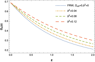
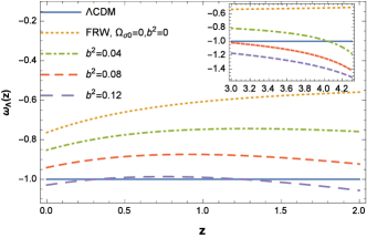
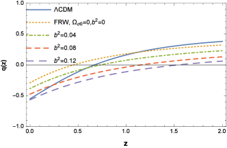
Fig. 1 : Upper panel: The redshift evolution of the density parameters $\Omega_{\Lambda}(z)$. Middle panel: The evolution of EoS parameter $\omega_{\Lambda}(z)$. Lower panel: The deceleration parameter $q(z)$ as a function of cosmic redshift $z$ for the different parameter $b^{2}$. Here we take $\Omega_{\Lambda}^{0}=0.69$ and $\Omega_{\sigma 0}=0.001$.

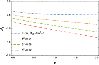
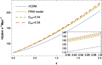
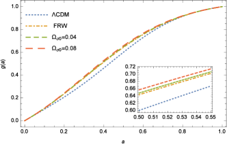
Fig. 2 : Upper panel: The evolution of squared sound speed $c_{s}^{2}$ as a function of cosmic redshift $z$ for the different parameter $b^{2}$ with $\Omega_{\Lambda}^{0}=0.69$ and $\Omega_{\sigma 0}=0.001$. Middle panel: Evolution of the Hubble parameter $H(z)$ as a function of cosmic redshift $z$ for the different parameter $\Omega_{\sigma 0}$ with $b^{2}=0.1$, $\Omega_{m0}=0.277$ and $H_{0}=72kms^{-1}Mpc^{-1}$. Lower panel: Time evolution of the growth factor as a function of the scale factor for the different cosmological models and comparing to the $\Lambda$CDM and FRW models. Auxiliary parameters are the same as shown in the middle panel of Fig. (2).

which is the squared sound speed for interacting ghost DE fluid. It may be mentioned that for causality and stability under perturbation it is required to satisfy the inequality condition $c_{s}^{2}\leq 1$ (Lixin et al, 2012).
In Fig. (1) we show the energy density of DE component $\Omega_{\Lambda}$ (upper panel), the evolution of the EoS parameter $\omega_{\Lambda}$ (middle panel), the deceleration parameter $q(z)$ (lower panel) while in Fig. (2) we show the squared sound speed $c_{s}^{2}$ (upper panel) and Hubble parameter $H$ (middle panel) as a function of the cosmic redshift $z$ for different values of the model parameters $b^{2}$ and $\Omega_{\sigma 0}$, and comparing to FRW ghost DE and $\Lambda$CDM cosmological models. In the case of the ghost DE model we have assumed the present values: $\Omega_{\sigma 0}=0.001$, $\Omega_{\Lambda}^{0}=0.69$ and $H_{0}=72~{}km/s~{}Mp/c$. Also for the case of $\Lambda$CDM model it is $\Omega_{\Lambda}^{0}=0.7$ and $\Omega_{m0}=0.3$. From figure (1) we see that for the case of $b^{2}\neq 0.12$, the EoS parameter for ghost DE model is always bigger than $\omega_{\Lambda}=-1$ and remains in the quintessence regime, i.e., $\omega_{\Lambda}>-1$ while for $b^{2}=0.12$, we see that $\omega_{\Lambda}$ of the ghost DE can cross the phantom divide. In the limiting case of the FRW Universe it was argued (Wei and Cai, 2008) that without interaction ($b^{2}=0$) $\omega_{\Lambda}$ is always larger than $-1$ and cannot cross the phantom divide while in the presence of the interaction the situation is changed. Recent studies have constructed $q(z)$ takeing into account that the strongest evidence of accelerations happens at redshift of $z\sim 0.2$. In order to do this, they have set $q(z)=1/2(q_{1}z+q_{2})/(1+z)^{2}$ to reconstruct it and after that they have obtained $q(z)\sim-0.31$ by fitting this model to the observational data (Gong and Wang, 2006). Under these conditions and considering bottom panel of figure (1), we give the present value of the deceleration parameter for the interacting ghost DE with $b^{2}=0.12$ is $q_{0}\simeq-0.56$, is significantly smaller than $q_{0}\sim-0.54$ for the $\Lambda$CDM cosmological model (Daly et al, 2008), as expected (see also figure (1)). Graphical analysis of $c_{s}^{2}$ shows that our theory could be unstable in FRW and BI models as shown in upper panel of Fig. (2). Furthermore, we would see that the non interacting ghost DE in FRW is more stable than the interacting ghost DE in an anisotropic Universe. It is also interesting to see how our models when compared with recent measurements of the Hubble parameter performed with the $\Lambda$CDM model. This comparison is done in figure 2 (middle panel), where we plot the evolution of $H(z)$ depends on the value of the $\Omega_{\sigma 0}$ parameter for the ghost DE and $\Lambda$CDM model considered in this work. It was observed that the Hubble parameter are bigger in these models compared to the $\Lambda$CDM model. Also, we can see that for the biggest value, the $\Omega_{\sigma 0}$ parameter is taken, and the biggest value of the Hubble expansion rate $H(z)$ is gotten.

3 Linear perturbation theory in ghost DE

The coupling between the dark components could significantly affect not only the expansion history of the Universe, but also the evolutions of the density perturbations, which would change the growth history of cosmic structure. The linear growth of perturbations for the large scale structures is derived from matter era, by calculating the evolution of the growth factor $g(a)$ in ghost DE models and compare it with the solution found for the $\Lambda$CDM model. The differential equation for $g(a)$ is given by (Pace et al, 2010, 2014; Percival, 2005)

$$g^{\prime\prime}(a)+(\frac{3}{a}+\frac{E^{\prime}(a)}{E(a)})g^{\prime}(a)-\frac{3}{2}\frac{\Omega_{m0}}{a^{5}E^{2}(a)}g(a)=0,$$ (26)

for the prime denoting the derivative with respect to $\ln a$ and $E(z)=H/H_{0}$ is the evolution of dimensionless Hubble parameter. For a non interacting DE model, by using Eqs. (14), (18) and (21), we solve numerically Eq. (26) for studying the linear growth with ghost DE in an anisotropic Universe. After that we compare the linear growth in the ghost DE model with the linear growths in the $\Lambda$CDM and FRW models. To evaluate the initial conditions, since we are in the linear regime, we take that the linear growth factor has a power law solution, $g(a)\propto a^{n}$, with $n>1$, then the linear growth should grow in time. In bottom panel of Fig. (2) we show the evolution of the linear growth factor $g(a)$ as a function of the scale factor. In the ghost DE model with $\Omega_{\sigma 0}\neq 0$, the growth factor evolves proportionally to the scale factor, as expected. In the FRW model ($\Omega_{\sigma 0}=0$), the growth factor evolves more slowly compared to the BI model because the FRW model dominates in the late time Universe. In the case of $\Lambda$CDM, $g(a)$ evolves more slowly than in the ghost DE of FRW model since the expansion of the Universe slows down the structure formation.

4 Bianchi type I field equations and ghost dark energy in Brans-Dicke theory

The BD theory with self-interacting potential is described by the action (Arik and Calik, 2006; Cataldo et al, 2001; Ebrahimi and Sheykhi, 2011)

$$S=\int d^{4}x\sqrt{g}\left(-\frac{1}{8\omega_{0}}\phi^{2}R+\frac{1}{2}g^{\mu\nu}\partial_{\mu}\phi\partial_{\nu}\phi+L_{m}\right),$$ (27)

where $\omega_{0}$ represent the constant BD parameter and $L_{m}$ the matter part of the Lagrangian. We have taken $8\pi G_{0}=c=1$. In particular we may expect that $\phi$ is spatially uniform, but varies slowly with time. The nonminimal coupling term $\phi^{2}R$ where $R$ is the Ricci scalar, replaces with the Einstein-Hilbert term $\frac{1}{G_{N}}R$ in such a way that $G_{eff}^{-1}=\frac{2\pi}{\omega_{0}}\phi^{2}$ where $G_{eff}^{-1}$ is the effective gravitational constant as long as the dynamical scalar field $\phi$ varies slowly. Using the principle of least action, we obtain the field equations

$$\phi G_{\mu\nu}=-8\pi T_{\mu\nu}^{m}-\frac{\omega_{0}}{\phi}\left(\phi_{,\mu}\phi_{,\nu}-\frac{1}{2}g^{\mu\nu}\phi_{,\gamma}\phi^{,\gamma}\right)$$ (28)

$$~{}~{}~{}~{}~{}~{}~{}~{}~{}~{}~{}~{}~{}~{}~{}~{}~{}~{}~{}~{}~{}~{}-\phi_{;\mu;\nu}+g_{\mu\nu}\Box\phi,$$ (29)

and

$$\Box\phi=\alpha^{\prime}T^{m\gamma}_{\gamma},$$ (30)

respectively, where $\alpha^{\prime}=\frac{8\pi}{2\omega_{0}+3}$ and $T^{m\gamma}_{\gamma}=g^{\mu\nu}T^{m}_{\mu\nu}$ is the trace of the matter stress-tensor which becomes calculated from $L_{m}$ through the definition $T^{m}_{\mu\nu}=\frac{2}{\sqrt{-g}}\frac{\delta}{\delta g_{\mu\nu}}[\sqrt{-g}L_{m}]$. For Bianchi type I spacetime, the field equations take the form

$$\frac{\phi^{2}}{4\omega_{0}}\left(3H^{2}-\sigma^{2}\right)-\frac{1}{2}\dot{\phi}^{2}-\frac{3H}{2\omega_{0}}\phi\dot{\phi}=\rho_{\Lambda}+\rho_{m},$$ (31)

$$\frac{-1}{4\omega_{0}}\left(2\dot{H}+3H^{2}+\sigma^{2}\right)\phi^{2}-\frac{1}{2}(1+\frac{1}{\omega_{0}})\dot{\phi}^{2}$$ (32)

$$~{}~{}~{}~{}~{}~{}~{}~{}~{}~{}~{}~{}~{}~{}~{}~{}~{}~{}~{}~{}~{}~{}+\frac{H}{\omega_{0}}\phi\dot{\phi}-\frac{1}{2\omega_{0}}\phi\ddot{\phi}=p_{\Lambda},$$ (33)

and the wave equation is

$$\ddot{\phi}+3H\dot{\phi}-\frac{1}{2\omega_{0}}\left(3\dot{H}+6H^{2}+\sigma^{2}\right)\phi=0.$$ (34)

As above, Eqs. (31), (33) and (34), are 3 independent equation which having unknown parameters such as $\phi$, $H$ and $\sigma$. To solve them we take $\sigma^{2}=\sigma_{0}^{2}H^{2}$ and $\phi=\phi_{0}a^{\epsilon}$ (Riazi and Nasr, 2000), where $\epsilon$ is any integer, implies that $\dot{\phi}=\epsilon H\phi$. So, Eq. (31) lead to

$$1+2\epsilon-\frac{2}{3}\omega_{0}\epsilon^{2}-\frac{\sigma_{0}^{2}}{3}=\frac{4\omega_{0}}{3H^{2}\phi^{2}}(\rho_{\Lambda}+\rho_{m}).$$ (35)

The fractional energy densities are defined as

$$\Omega_{m}=\frac{\rho_{m}}{\rho_{cr}}=\frac{4\omega_{0}\rho_{m}}{3\phi^{2}H^{2}},$$ (36)

$$\Omega_{\Lambda}=\frac{\rho_{\Lambda}}{\rho_{cr}}=\frac{4\omega_{0}\rho_{\Lambda}}{3\phi^{2}H^{2}}=\frac{4\omega_{0}\alpha}{3\phi^{2}H},$$ (37)

where $\rho_{cr}=\frac{3\phi^{2}H^{2}}{4\omega_{0}}$. Therefore, Eq. (35) give

$$\Omega_{\Lambda}+\Omega_{m}=1+2\epsilon-\frac{2}{3}\omega_{0}\epsilon^{2}-\Omega_{\sigma 0}.$$ (38)

In the following, we take the time derivative of (35), after using (38), so

$$\frac{{H^{\prime}(z)}}{H}=\frac{3}{2(1+z)}$$ (39)

$$~{}~{}~{}~{}~{}~{}\times\left(1+\frac{2}{3}\epsilon+\frac{\Omega_{\Lambda}\omega_{\Lambda}}{1+2\epsilon-\frac{2}{3}\omega_{0}\epsilon^{2}-\Omega_{\sigma 0}}\right).$$ (40)

For the case of $\epsilon=0$, the above equation reduce to (18). Here by combining (8) with (16) and also (39), we obtain the EoS parameter in BD theory as

$$\omega_{\Lambda}(z)=\frac{1+2\epsilon-\frac{2}{3}\omega_{0}\epsilon^{2}-\Omega_{\sigma 0}}{-2(1+2\epsilon-\frac{2}{3}\omega_{0}\epsilon^{2}-\Omega_{\sigma 0})+\Omega_{\Lambda}(z)}$$ (41)

$$~{}~{}~{}~{}\times\bigg{(}1-\frac{2\epsilon}{3}+\frac{2b^{2}(1+2\epsilon-\frac{2}{3}\omega_{0}\epsilon^{2}-\Omega_{\sigma 0})}{\Omega_{\Lambda}(z)}\bigg{)}.$$ (42)

The solar-system experiments give the lower bound for the value of $\omega_{0}$ to be $\omega_{0}>40000$ (Ohta, 2011). However, when probing the larger scales, the limit obtained will be weaker than this result. It was shown (Acquaviva and Verde, 2007) that $\omega_{0}$ can be smaller than 40000 on the cosmological scales. Also, Sheykhi et al. (Shekhi et al, 2013) obtained the result for the value of $\epsilon$ is $\epsilon<0.01$. The ghost DE model in BD framework has an interesting feature compared to the ghost DE model in BI Universe. In the case of $b^{2}=0$, the EoS parameter of in the BD framework, requiring condition $\omega_{\Lambda}<-1$ leads to $(1+2\epsilon-\frac{2}{3}\omega_{0}\epsilon^{2}-\Omega_{\sigma 0})(3+2\epsilon)<3\Omega_{\Lambda}$. We can also obtain the evolution behavior of the DE. Taking the derivative of (36) as $\dot{\Omega}_{\Lambda}=-\Omega_{\Lambda}H(\frac{\dot{H}}{H^{2}}+2\epsilon)$ and using relation $\dot{\Omega}_{\Lambda}=-H(z)(1+z)\Omega_{\Lambda}^{\prime}(z)$, it follows that

$$\Omega_{\Lambda}^{\prime}(z)=-\frac{3\Omega_{\Lambda}}{1+z}\bigg{(}\frac{\Omega_{\Lambda}-1-2\epsilon+\frac{2}{3}\omega_{0}\epsilon^{2}+\Omega_{\sigma 0}}{-2(1+2\epsilon-\frac{2}{3}\omega_{0}\epsilon^{2}-\Omega_{\sigma 0})+\Omega_{\Lambda}(z)}\bigg{)}$$ (43)

$$\bigg{(}1-\frac{2}{3}\epsilon+b^{2}(1+2\epsilon-\frac{2}{3}\omega_{0}\epsilon^{2}-\Omega_{\sigma 0})\bigg{)}.$$ (44)

Now, the deceleration parameter in BD theory is obtained as

$$q(z)=\frac{1}{2}+\epsilon+\frac{3\Omega_{\Lambda}}{-2(1+2\epsilon-\frac{2}{3}\omega_{0}\epsilon^{2}-\Omega_{\sigma 0})+\Omega_{\Lambda}(z)}$$ (45)

$$~{}~{}~{}~{}~{}\times\bigg{(}1-\frac{2}{3}\epsilon+\frac{b^{2}(1+2\epsilon-\frac{2}{3}\omega_{0}\epsilon^{2}-\Omega_{\sigma 0})}{\Omega_{\Lambda}(z)}\bigg{)},$$ (46)

where $\Omega_{\Lambda}$ is given by Eq. (43). A same steps as the pervious section can be followed to obtain the squared sound speed $c_{s}^{2}$ for Brans-Dicke theories. Taking time derivative of Eq. (41) and replacing them into the Eq. (23) it is a matter of calculation to show that

$$c_{s}^{2}=\frac{\gamma}{3\Omega_{\Lambda}(2\gamma+\Omega_{\Lambda})^{2}}\bigg{[}(2\gamma+\Omega_{\Lambda})(6b^{2}\gamma+\epsilon^{\prime}\Omega_{\Lambda})$$ (47)

$$+\frac{(\gamma(\epsilon^{\prime}+3b^{2})+\epsilon^{\prime}\Omega_{\Lambda})(\epsilon^{\prime}\Omega^{2}_{\Lambda}+12\gamma b^{2}(\gamma+\Omega_{\Lambda}))}{\gamma(-3+3b^{2}-2\epsilon)-3\Omega_{\Lambda}}\bigg{]},$$ (48)

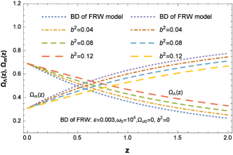
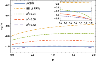
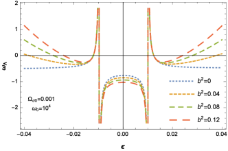
Fig. 3 : Top panel: DE density parameters $\Omega_{\Lambda}$ and $\Omega_{m}$ for the interacting ghost DE of BD theory with different $b^{2}$. The evolutionary trajectories of $\omega_{\Lambda}$ for the interacting ghost DE with $\epsilon=0.003$ with different values $b^{2}$ as a function of cosmic redshift $z$ (middle panel) and in terms of $\epsilon$ (lower panel). Here we choose $\omega_{0}=10^{4}$, $\Omega^{0}_{\Lambda}=0.69$ and $\Omega_{\sigma 0}=0.001$.

Fig. 4 : The best fits of $\epsilon$ with anisotropy parameter for the interacting GDE model. The results given by current only are $z=1$, $H_{0}=72~{}km/s/Mpc$, $b^{2}=0.1$, and $\Omega_{m0}=0.277$.

where $\gamma=-1-2\epsilon+\frac{2}{3}\omega_{0}\epsilon^{2}+\Omega_{\sigma 0}$ and $\epsilon^{\prime}=-3+2\epsilon$. In Fig. 3 we plot the energy density of DE component $\Omega_{\Lambda}(z)$ and the energy density of DM $\Omega_{m}(z)$ (upper panel), the redshift evolution of the equation of state $\omega_{\Lambda}(z)$ as a function of both $z$ and $\epsilon$ in middle (lower panel) while the parameter $\epsilon$ versus the anisotropy parameter is plotted in figure (4). In Fig. 5 we plot the deceleration parameter (upper panel) and the squared sound speed (middle panel) as a function of the cosmic redshift $z$ for different parameter $b^{2}$ in BD theory. In the case of the ghost DE of BD theory we select the model parameter as $\Omega_{\sigma 0}=0.001$, $\Omega_{\Lambda}^{0}=0.69$, $\epsilon=0.003$ and $\omega_{0}=10^{4}$. Fig. 3 (upper) indicates that at the late time $\Omega_{\Lambda}\rightarrow 0.7$ while for the case of the energy density of DM $\Omega_{m}\rightarrow 0.3$, which is similar to the behaviour of the original ghost DE in previous section. From Fig. 3 (middle) we observe that for $b^{2}=\Omega_{\sigma 0}=0$, the EoS parameter of BD theory translates the Universe from low quintessence region towards high quintessence region. But for $b^{2}\neq 0.12$, $\omega_{\Lambda}$ increases from phantom region at early times and approaches to quintessence region at late times. Also from Fig. 3 we see that for $b^{2}=0.12$, $\omega_{\Lambda}$ of the interacting ghost DE in BD theory can cross the phantom divide and eventually the Universe approaches low phantom phase of expansion at late time. The lower of figure (3) indicates that one can generate a phantom-like behavior provided $-0.01<\epsilon<0.01$ which this point is completely compatible with the Ref. (Shekhi et al, 2013). For a better insight, we plotted $\epsilon$ against the anisotropy parameter as shown in figure 4. The sweet spot is estimated to be $z=1$.
We figure out that the behaviour of the deceleration parameter for the best-fit Universe is quite different from the $\Lambda$CDM cosmology as shown in Fig. 5 (upper panel). We can also see that the best fit values of transition redshift and current deceleration parameter with ghost DE of BD theory are $z=2.13^{+0.84+1.28}_{-0.00-0.55}$ and $q_{0}=-1.32^{+00+0.10}_{-0.07-0.17}$ which is matchable with the observations (Ishida et al, 2008) while for the case of $\Lambda$CDM, where $z\sim 0.67$ and $q_{0}=-0.54$. We can see that increasing $b^{2}$ decreases the value of $q(z)$. The evolution of $c_{s}^{2}$ against $z$ is plotted in Fig. 5 (middle panel) for different values of the coupling parameter $b^{2}$. The figure reveals that $c_{s}^{2}$ is always negative and thus, as the previous case, a background filled with the interacting ghost DE seems to be unstable against the perturbation. This implies that we cannot obtain a stable ghost DE dominated Universe in BD theory, which are in agreement with (Fayaz, 2016; Myung, 2007). One important point is the sensitivity of the instability to the coupling parameter $b^{2}$. The larger $b^{2}$, leads to more instability against perturbations.
In the following, we study the capability of the $H(z)$ measurements in constraining DE models in BD theory. The evolution of Hubble parameter $H(z)$ in ghost DE model with BD theory is obtained by using Eqs. (8) and (35) as follows

$$H=\frac{H_{0}}{-2\gamma}\bigg{(}-\Omega_{m0}-\gamma$$ (49)

$$~{}~{}~{}~{}~{}~{}~{}~{}+\sqrt{(-\gamma-\Omega_{m0})^{2}-4\gamma\Omega_{m0}(1+z)^{3}}\bigg{)}.$$ (50)

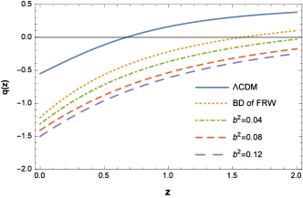
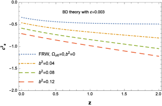
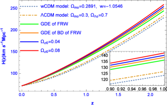
Fig. 5 : Top panel: The evolution of $q(z)$ in terms of $z$ for the interacting ghost DE of BD theory with different $b^{2}$. Middle panel: The evolution of $c_{s}^{2}$ as a function of cosmic redshift $z$ for the different parameter $b^{2}$ with $\Omega^{0}_{\Lambda}=0.69$ and $\Omega_{\sigma 0}=0.001$. Lower panel: Hubble expansion parameter in terms of redshift for the different parameter $\Omega_{\sigma 0}$ with $b^{2}=0.1$, $\Omega_{m0}=0.277$, $H_{0}=72kms^{-1}Mpc^{-1}$, $\epsilon=0.003$ and $\omega_{0}=10^{4}$.

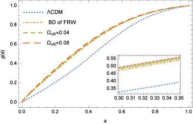
Fig. 6 : Evolution of growth function $g(a)$ in terms of $a$ for the different $\Omega_{\sigma 0}$ and comparing to the $\Lambda$CDM and FRW models in ghost DE of BD theory.

The behaviour of the Hubble parameter is similar to that of the matter density parameters ($\Omega_{m}$), which is expected because DE comes to dominate the evolution of the Hubble parameter only at very low redshift. We elect three specific DE models as representatives of cosmological models in order to make the analysis. They are the $\Lambda$CDM, $w$CDM, ghost DE of BD theory in BI (FRW) models. We consider to use the SGL+CBS (the strong gravitational lensing, the cosmic microwave background, baryon acoustic oscillations and type Ia supernova) data to constrain the $w$CDM and ghost DE models and we take $\Omega_{m0}=0.2891$ and $w=-1.0546$ (Cui et al, 2015). As a matter of fact we can also see the lower panel of Fig. 5 that in a BI model although ghost DE model performs a little poorer than $\Lambda$CDM model, but it performs better than ghost DE in BD theory. Also, from this figure we can understand the Hubble parameter in ghost DE of BD theory in BI are bigger than in the ghost DE of FRW, $\Lambda$CDM and $w$CDM models. The larger the Hubble expansion rate $H(z)$ is taken, the bigger the anisotropy parameter $\Omega_{\sigma 0}$ can reach. Therefore, from the above analysis, we will figure out that both the parameters, $b^{2}$ and $\Omega_{\sigma 0}$, can impact the cosmic expansion history in the interacting ghost DE of BD theory in BI model.
In Fig. (6) we show the effects of anisotropy on the growth factor in ghost DE of BD theory for the DE models considered in this work, as compared to the $\Lambda$CDM model. Generally, the $\Lambda$CDM model observe less growth compared to the ghost DE of BD theory in an anisotropic Universe. Therefore the growth factor $g(a)$ for the $\Lambda$CDM Universe will always fall behind the ghost DE models.
The theoretical distance modulus $\mu_{th}(z)$ is defined as (Wang et al, 2016)

$$\mu_{th}(z)=5\log_{10}\frac{d_{L}(z)}{Mpc}+25,$$ (51)

where $d_{L}(z)=(1+z)\int{{}^{z}_{0}H^{-1}(z^{\prime})}dz^{\prime}$ is the luminosity distance. The structure of the anisotropies of the CMB radiation depends on two eras in cosmology, such as last scattering and today. We can also measure $d_{L}(z)$ through the Hubble parameter by using the Eq. (14). Figure 7 presents the distance modulus with the best fit of our model and the best fit of the $\Lambda$CDM model. From Fig. (7) we can observe the Universe is accelerating expansion. In all, current data are unable to discriminate between the popular $\Lambda$CDM, FRW and our interaction models.

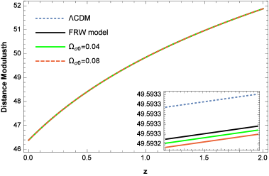
Fig. 7 : Distance modulus for the best fit model $\Omega_{m0}=0.277$, $H_{0}=72~{}km/s/Mpc$, $b^{2}=0.1$, and the $\Lambda$CDM model, $\Omega_{m0}=0.3$, $H_{0}=72~{}km/s/Mpc$ and $\Omega^{0}_{\Lambda}=0.7$.

5 Conclusion

In this work we studied the linear evolution of structure formation in interacting ghost DE models within the framework of Brans-Dicke theory. first of all, we initiate our analysis by studying the effects of anisotropy on the background expansion history of the growth factor. We obtained the evolution of density parameter $\Omega_{\Lambda}$, the equation of state parameter $\omega_{\Lambda}$, the deceleration parameter $q$ and the squared sound speed $c_{s}^{2}$ for both the ghost DE and Brans-Dicke theory with respect to the cosmic redshift function. At first, the EoS parameter of the ghost DE and BD theory models in the case of $b^{2}\neq 0.12$, cannot cross the phantom divide while it for $b^{2}=0.12$ can cross the phantom divide line. Beside, increasing of the anisotropy and the interaction parameter is increased the phantomic. Then, the evolution of the interacting ghost DE density parameter in BD theory is depend on the anisotropy density parameter $\Omega_{\sigma 0}$ and the coupling constant $b^{2}$. On the basis of the above considerations, it seems reasonable to investigate an anisotropic Universe, in which the present cosmic acceleration is followed by a decelerated expansion in an early matter dominant phase. In other words, it indicates that the values of transition scale factor and current deceleration parameter are $z=0.74^{+0.40+0.78}_{-0.00-0.28}$ and $q_{0}=-0.37^{+00+0.08}_{-0.09-0.19}$ for the case of ghost DE, $z=2.13^{+0.84+1.28}_{-0.00-0.55}$ and $q_{0}=-1.32^{+00+0.10}_{-0.07-0.17}$ for the case of ghost DE with BD theory while for the case of $\Lambda$CDM model, $z=0.67$ and $q_{0}=-0.54$ which is consistent with observations (Gong and Wang, 2006; Myung, 2007). We have used the squared sound speed $c_{s}^{2}$ as the main factor to study the stability of the ghost DE in BD theory. As a result, a BI Universe filled with DM and ghost DE component in BD gravity can lead to an unstable interacting ghost DE dominated Universe. In this case the frequency of the oscillations becomes purly imaginary and the density perturbations will grow with time.
Then, we analyzed $H(z)$ and compare the results with observational data. We found that, by choosing appropriate values of constant parameters, we figure out our model has more agreement with observational data than $\Lambda$CDM. Furthermore, we show that in anisotropic Universe with ghost DE of BD theory, the Hubble parameter are bigger than the ghost DE of FRW, $\Lambda$CDM and $w$CDM models. It was observed that the larger the Hubble expansion rate $H(z)$ is taken, the bigger the anisotropy parameter $\Omega_{\sigma 0}$ can reach. Finally the effects of anisotropy on the growth of structures in linear regime is investigated and we compared the linear growth in the ghost DE and BD theory with the linear growth in the FRW and $\Lambda$CDM models which in the $\Lambda$CDM, the growth factor evolves more slowly compared to the ghost DE of FRW in BD theory because the cosmological constant dominates in the late time universe. Also, in the ghost DE of FRW in BD theory, the growth factor evolves more slowly compared to the ghost DE models in anisotropic Universe. Therefore due to BD theory the growth factor $g(a)$ for the $\Lambda$CDM Universe will always fall behind the ghost DE models in an anisotropic Universe.

References

- Reiss et al (1998) A.G. Reiss, A.V. Filippenko, P. Challis et al., Astron. J. 116, 1009 (1998).
- Perlmutter et al (1999) S. Perlmutter, G. Aldering, G. Goldhaber, et al. Astrophys. J. 517, 565 (1999).
- Peebles and Ratra (2003) P.J. Peebles and B. Ratra, Rev. Mod. Phys. 75, 559 (2003).
- Caldwell et al (1998) R.R. Caldwell, R. Dave and P.J. Steinhardt, Phys. Rev. Lett. 80, 1582 (1998).
- Nojiri and Odintsov (2003) S. Nojiri and S.D. Odintsov, Phys. Lett. B 562, 147 (2003).
- Khodam-Mohammadi et al (2012) A. Khodam-Mohammadi, M. Malekjani, M. Monshizadeh, Mod. Phys. Lett. A 27, 1250100 (2012).
- Sadeghi et al (2008) J. Sadeghi, M.R. Setare, A. Banijamali and F. Milani, Phys. Lett. B 662, 92 (2008).
- Urban and Zhitnitsky (2010) F.R. Urban and A.R. Zhitnitsky, Phys. Lett. B 688, 9 (2010).
- Ohta (2011) N. Ohta, Phys. Lett. B 695, 41 (2011).
- Witten (1979) E. Witten, Nucl. Phys. B 156, 269 (1979).
- Veneziano (1979) G. Veneziano, Nucl. Phys. B 159, 213 (1979).
- Nath and Arnowitt (1981) P. Nath and R.L. Arnowitt, Urrent Algebra And The Theta Vacuum, Phys. Rev. D 23, 473 (1981).
- Kawarabayashi and Ohta (1980) K. Kawarabayashi and N. Ohta, Nucl. Phys. B 175, 477 (1980).
- Piazza and Tsujikawa (2004) F. Piazza and S. Tsujikawa, JCAP 0407, 004 (2004).
- Zhitnitsky (2010) A.R. Zhitnitsky, Phys. Rev. D 82, 103520 (2010).
- Holdom (2011) B. Holdom, Phys. Lett. B 697, 351 (2011).
- Zhitnitsky (2011) A.R. Zhitnitsky, Phys. Rev. D 84, 124008 (2011).
- Brans and Dicke (1961) C.H. Brans and R.H. Dicke, Phys. Rev. 124, 925 (1961).
- Bertotti (2003) B. Bertotti, L. Iess and P. Tortora, Nature (London) 425, 374 (2003).
- Alavirad and Sheykhi (2014) H. Alavirad and A. Sheykhi, Phys. Lett. B 734, 148 (2014).
- Ebrahimi and Sheykhi (2011) E. Ebrahimi and A. Sheykhi, Int. J. Mod. Phys. D 20, 2369 (2011).
- Saaidi et al (2012) Kh. Saaidi, A. Aghamohammadi, B. Sabet and O. Farooq, Int. J. Mod. Phys. D 21, 1250057 (2012).
- Saha (2006) B. Saha, Astrophys. Space Sci. 302, 83 (2006).
- Pradhan and Singh (2004) A. Pradhan, S.K. Singh, Int. J. Mod. Phys. D 13, 503 (2004).
- Saha (2006) B. Saha, Int. J. Theor. Phys. 45, 983 (2006).
- Shamir (2010) M.F. Shamir, Astrophys. Space Sci. 330, 183 (2010).
- Yadav and saha (2012) A.K. Yadav, B. Saha, Astrophys. Space Sci. 337, 759 (2012).
- Pradhan and Pandey (2006) A. Pradhan and P. Pandey, Astrophys. Space Sci. 301, 221 (2006).
- Aluri et al (2013) P. Aluri et al., J. Cosmol. Astropart. Phys. 12, 3 (2013).
- Sharif and Waheed (2012) M. Sharif, Saira Waheed, Eur. Phys. J. C, 72, 1876 (2012).
- Ram (1983) S. Ram, Astrophys. Space. Sci. 94, 307 (1983).
- Farasat Shamir and Ahmad Bhatti (2012) M. Farasat Shamir, Akhlaq Ahmad Bhatti, Can. J. Phys. 90, 193 (2012).
- Hossienkhani (2016) H. Hossienkhani, Astrophys. Space Sci. 361, 136 (2016).
- Hossienkhani and Pasqua (2014) H. Hossienkhani and A. Pasqua, Astrophys. Space Sci. 349, 39 (2014); Kh. Saaidi and H. Hossienkhani, Astrophys. Space Sci. 333, 305 (2011).
- Borges and Carneiro (2005) H.A. Borges, S. Carneiro, Gen. Rel. Grav. 37, 1385 (2005).
- Reiss et al (2011) A.G. Riess, L. Macri, S. Casertano et al., Astrophys J, 730, 119 (2011).
- Spergel et al (2007) D.N. Spergel et al., Astrophy. J. Suppl. 170, 377 (2007).
- Chen et al (2003) G. Chen, J.R. Gott, B. Ratra, PASP, 115, 1269 (2003).
- Gott et al (2001) J.R. Gott, M.S. Vogeley, S. Podariu, B. Ratra, ApJ, 549, 1 (2001).
- Wang et al (2005) B. Wang, Y. Gong and E. Abdalla, Phys. Lett. B 624, 141 (2005).
- Sen and Pavón (2008) Anjan A. Sen, D. Pavón, Phys. Lett. B 664, 7 (2008).
- Lixin et al (2012) X. Lixin, W. Yuting and N. Hyerim, Eur. Phys. J. C 72, 1931 (2012).
- Pace et al (2010) F. Pace, J.C. Waizmann, M. Bartelmann, MNRAS, 406, 1865 (2010).
- Pace et al (2014) F. Pace, L. Moscardini, R. Crittenden, M. Bartelmann, V. Pettorino, MNRAS, 437, 547 (2014).
- Percival (2005) W.J. Percival, A. A, 443, 819 (2005).
- Wei and Cai (2008) H. Wei and R.G. Cai, Phys. Lett. B 660, 113 (2008).
- Gong and Wang (2006) Y.G. Gong, A. Wang, Phys. Rev. 75, 043520 (2006).
- Daly et al (2008) R.A. Daly et al., J. Astrophys. 677, 1 (2008).
- Arik and Calik (2006) M. Arik, M.C. Calik, Mod. Phys. Lett. A 21, 1241 (2006).
- Cataldo et al (2001) M. Cataldo, S. del Campo, P. Salgado, Phys. Rev. D 63, 063503 (2001).
- Ebrahimi and Sheykhi (2011) E. Ebrahimi, A. Sheykhi, Phys. Lett. B 706, 19 (2011).
- Riazi and Nasr (2000) N. Riazi, B. Nasr, Astrophys. Space Sci. 271, 237 (2000).
- Acquaviva and Verde (2007) V. Acquaviva, L. Verde, JCAP 0712, 001 (2007).
- Shekhi et al (2013) A. Sheykhi, E. Ebrahimi and Y. Yousefi, Can. J. Phys 91, 662 (2013).
- Ishida et al (2008) E.E.O. Ishida et al., Astropart. Phys, 28, 547 (2008).
- Fayaz (2016) V. Fayaz, Astrophys. Space Sci. 361, 86 (2016).
- Myung (2007) Y.S. Myung, Phys. Lett. B 652, 223 (2007); K.Y. Kim, H.W. Lee and Y.S. Myung, Phys. Lett. B 660, 118 (2008).
- Cui et al (2015) J.L. Cui, Y.Y. Xu, J.F. Zhang, X. Zhang, Sci. China. Phys. Mech. Astron, 58, 110402 (2015).
- Wang et al (2016) S. Wang, Y. Wang and M. Li, (2016), arXiv:1612.00345v1.