Pion-nucleon scattering in covariant baryon chiral perturbation theory with explicit Delta resonances

Abstract

We present the results of a third order calculation of the pion-nucleon scattering amplitude in a chiral effective field theory with pions, nucleons and delta resonances as explicit degrees of freedom. We work in a manifestly Lorentz invariant formulation of baryon chiral perturbation theory using dimensional regularization and the extended on-mass-shell renormalization scheme. In the delta resonance sector, the on mass-shell renormalization is realized as a complex-mass scheme. By fitting the low-energy constants of the effective Lagrangian to the $S$- and $P$-partial waves a satisfactory description of the phase shifts from the analysis of the Roy-Steiner equations is obtained. We predict the phase shifts for the $D$ and $F$ waves and compare them with the results of the analysis of the George Washington University group. The threshold parameters are calculated both in the delta-less and delta-full cases. Based on the determined low-energy constants, we discuss the pion-nucleon sigma term. Additionally, in order to determine the strangeness content of the nucleon, we calculate the octet baryon masses in the presence of decuplet resonances up to next-to-next-to-leading order in SU(3) baryon chiral perturbation theory. The octet baryon sigma terms are predicted as a byproduct of this calculation.

I Introduction

Elastic pion-nucleon ($\pi N$) scattering has been studied extensively since the middle of the last century (see e.g. Refs. Bransden:1973 ; Hohler:1983 ), not only due to the wealth of experimental data, but also because of its importance for our understanding of chiral dynamics of quantum chromodynamics (QCD). From the theory side, in order to describe such a fundamental process, dispersion relations for $\pi N$ scattering have been investigated several decades ago Chew:1957zz ; Hamilton:1963zz ; Steiner:1970mh and many phenomenological models and different approaches have been proposed (see, e.g., Refs. Olsson:1975th ; Bofinger:1991ed ; Gross:1992tj ; Schutz:1998jx ; Krehl:1999ak ; Gasparyan:2003fp ; Gasparyan:2010xz ; Ronchen:2012eg ). Roy-Steiner equations for the pion-nucleon scattering have been also analysed recently Ditsche:2012fv ; Hoferichter:2015dsa ; Hoferichter:2015tha ; Hoferichter:2015hva . In the low-energy region a systematic and powerful tool to study $\pi N$ scattering is provided by chiral perturbation theory (ChPT)  Weinberg:1978kz ; Gasser:1983yg ; Gasser:1984gg ; Scherer:2012xha . An extension of the range of applicability of chiral effective field theory (EFT) beyond the low-energy region has been also suggested in the recent work of Ref. Epelbaum:2015vea .

ChPT is the EFT of QCD in the low-energy region, which is widely used in modern hadronic physics. It has the same symmetries as its underlying theory and is based on an expansion in powers of small quark masses and external momenta, collectively denoted by $p$. According to the power counting rules of ChPT, powers of $p$ are assigned to Feynman diagrams and used to estimate the relative importance of their contributions in physical quantities. Hence, low-energy physical quantities, which can not be obtained within perturbative QCD, are calculated in a perturbative expansion in powers of $p$. Purely mesonic ChPT, the theory of Goldstone bosons only, has been very successful Gasser:1983yg ; Gasser:1984gg . However, in baryon chiral perturbation theory (BChPT), which additionally takes baryons into account, the power counting becomes subtle due to the non-zero baryon masses in the chiral limit. A first attempt to study elastic $\pi N$ scattering using BChPT was made in Ref. Gasser:1987rb . Therein, the power counting rule was shown to be broken when the baryon propagators are involved in loop integrals, namely loop diagrams give contributions of orders lower than assigned by the power counting.

To remedy this power counting breaking (PCB) issue, several approaches were proposed during the last decades. The most well-known approach is to calculate physical quantities within heavy baryon chiral perturbation theory (HBChPT) Jenkins:1990jv ; Bernard:1992qa . In order to restore the power counting, a simultaneous expansion in $p$ and in inverse powers of the baryon mass is performed. Within this framework $\pi N$ scattering was analysed in detail up to order ${\cal O}(p^{3})$ Mojzis:1997tu ; Fettes:1998ud and later up to order ${\cal O}(p^{4})$ Fettes:2000xg . A good description of partial wave phase shifts has been achieved near threshold. However, the non-relativistic heavy baryon expansion distorts the analytic structure of the amplitudes, e.g. the location of the poles of baryon propagators are shifted, and also convergence problems are encountered in certain low-energy regions, e.g. for the scalar form factor of the nucleon at $t=4M_{\pi}^{2}$ Becher:1999he . It should be noted, however, that the proper analytic structure can be regained if one includes subleasing terms in the heavy baryon propagator, see e.g. Bernard:1993ry . In any case, it is of interest to treat the PCB problem within covariant BChPT. A pioneering work in Ref. Ellis:1997kc restored the power counting by keeping only the so-called soft parts of the Feynman diagrams. Successively, a much more elegant approach, known as infrared regularization (IR), was proposed in Ref. Becher:1999he and later extended/reformulated in Refs. Goity:2001ny ; Bernard:2003xf ; Schindler:2003xv ; Bruns:2008ub . All the Feynman integrals in the IR regularization scheme are divided into infrared singular parts, respecting the power counting rules, and infrared regular parts, possibly violating them, and therefore the latter are discarded by means of absorbing them in (an infinite number of) the low-energy constants (LECs) of the effective Lagrangian. By making use of the IR scheme, $\pi N$ scattering has been studied up to ${\cal O}(p^{4})$ order Becher:2001hv (see also Ref. Alarcon:2011kh for ${\cal O}(p^{3})$ order calculation). Besides, the analyses of the isospin violation and the SU(3) sector of BChPT have also been considered in Refs. Hoferichter:2009gn and Mai:2009ce , respectively. However, the IR regularization has its own drawbacks: the presence of an unphysical $u$-channel cut Becher:1999he ; Ellis:1997kc and the prediction of a large discrepancy of the Goldberger-Treiman (GT) relation Alarcon:2011kh . All these problems are due to dropping the entire infrared regular parts.

The extended-on-mass-shell (EOMS) scheme, developed in Refs. Gegelia:1999gf ; Gegelia:1999qt ; Fuchs:2003qc , is an alternative approach to solve the PCB problem. It removes the power counting breaking terms (PCBT) at the level of amplitudes (or observables) by absorbing them into the renormalization of LECs of the effective Lagrangian. This is due to the fact that the PCBTs are polynomials of momenta and/or quark masses. The EOMS scheme preserves the analytic structure of the physical quantities, e.g. scattering amplitudes. $\pi N$ scattering has been calculated using EOMS scheme in Ref. Alarcon:2012kn up to order ${\cal O}(p^{3})$ and in Ref. Chen:2012nx up to order ${\cal O}(p^{4})$. Contributions to the scattering amplitudes obtained in those works possess the correct power counting and correct analytic properties. Moreover, the existing results of partial wave analysis are described well, and remarkably, reasonable predictions for discrepancy of GT relation and the pion-nucleon sigma term $\sigma_{\pi N}$ are obtained. Nevertheless, as pointed out in Ref. Alarcon:2012kn , the convergence of the chiral expansion of the ${\cal O}(p^{3})$ order $\pi N$ scattering amplitude within EOMS scheme is questionable when the $\Delta(1232)$ is not taken as an explicit degree of freedom. This implies the necessity of including the $\Delta(1232)$ resonances as explicit degrees of freedom in the effective Lagrangian, together with nucleons and pions.

In this work, we present the full third order (leading one loop) calculation of the pion-nucleon scattering amplitude in a manifestly Lorentz invariant formulation of BChPT with explicit deltas. We perform renormalization using the EOMS scheme such that the power counting violating terms are dealt with properly. The $S$- and $P$-wave phase shifts are extracted from the manifestly Lorentz invariant amplitudes and then fitted to the phase shifts obtained from the recent Roy-Steiner (RS) equation analysis of $\pi N$ scattering Hoferichter:2015hva such that all involved LECs are determined. Based on the obtained LECs, we predict the $D$- and $F$-wave phase shifts and compare them with the results of the George Washington University (GWU) group analysis SAID . The threshold parameters are determined for both the delta-less and delta-full cases. In addition, we discuss the pion-nucleon sigma term and the strangeness content of the nucleon in SU(3) BChPT.

This paper is organized as follows. In Section II we introduce the notations and the kinematics for the pion-nucleon scattering amplitudes. Terms of the chiral effective Lagrangian that are needed for our third order calculation of the pion-nucleon scattering amplitude are specified in Section III. Contributions of tree and one loop diagrams in the scattering amplitude are discussed in Section IV. Renormalization of the one loop diagrams and the definitions of the pion-nucleon, $g_{\pi N}$, and pion-nucleon-delta, $g_{\pi N\Delta}$, couplings are given in Section V. Section VI contains the extraction of the phase shifts. The baryon sigma terms and the strangeness content of the nucleon are discussed in Section VII. We summarize our results in Section  VIII and the appendices contain explicit expressions of various quantities as well as other technicalities.

II Formal aspects of elastic pion-nuleon scattering

II.1 Kinematics and the structure of the amplitude

The on-shell Lorentz- and time-reversal invariant $T$-matrix for the elastic scattering process $\pi^{a}(q)+N(p)\to\pi^{a^{\prime}}(q^{\prime})+N(p^{\prime})$, with Cartesian isospin indices $a^{\prime}$ and $a$, depends on three Mandelstam variables

$$s=(p+q)^{2}\ ,\quad t=(p-p^{\prime})^{2}\ ,\quad u=(p-q^{\prime})\ ,$$ (1)

subject to the constraint

$$s+t+u=2m_{N}^{2}+2M_{\pi}^{2}\,,$$ (2)

with $m_{N}$ and $M_{\pi}$ the physical masses of the nucleon and the pion, respectively. In the isospin limit, the amplitude $T^{a^{\prime}a}_{\pi N}(s,t,u)$ can be parameterized as

$$T_{\pi N}^{a^{\prime}a}(s,t,u)=\chi_{N^{\prime}}^{\dagger}\left\{\delta_{a^{\prime}a}T^{+}(s,t,u)+\frac{1}{2}[\tau_{a^{\prime}},\tau_{a}]T^{-}(s,t,u)\right\}\chi_{N}\ ,$$ (3)

where $\tau_{i}$ are the Pauli matrices and $\chi_{N}$, $\chi_{N^{\prime}}$ denote nucleon iso-spinors. Unless stated otherwise, the argument $u$ is always to be understood as a function of $s$ and $t$, $u(s,t)=2m_{N}^{2}+2M_{\pi}^{2}-s-t$. The Lorentz decomposition of the invariant amplitudes $T^{\pm}$ reads

$$T^{\pm}(s,t,u)=\bar{u}^{(s^{\prime})}(p^{\prime})\left\{D^{\pm}(s,t,u)-\frac{1}{4m_{N}}[\not{q}^{\prime},\not{q}]B^{\pm}(s,t,u)\right\}u^{(s)}(p)\ ,$$ (4)

with the superscript $(s^{\prime})$, $(s)$ denoting the spins of the Dirac spinors $\bar{u}$, $u$, respectively. The Lorentz decomposition is not unique, a popular alternative form is

$$T^{\pm}(s,t,u)=\bar{u}^{(s^{\prime})}(p^{\prime})\left\{A^{\pm}(s,t,u)+\frac{1}{2}\left(\not{q}^{\prime}+\not{q}\right)B^{\pm}(s,t,u)\right\}u^{(s)}(p)\ .$$ (5)

Furthermore, $A^{\pm}$ can be related to $B^{\pm}$ and $D^{\pm}$ via $A^{\pm}=D^{\pm}-\nu B^{\pm}$ with $\nu\equiv(s-u)/(4m_{N})$. Nevertheless, it is well known that the decomposition in terms of $D$ and $B$, i.e. Eq. (4), is better suited to perform the chiral expansion of the invariant amplitudes, while there exists cancellations between power counting violating contributions from $A$ and $B$.

The whole $T$-matrix $T_{\pi N}^{a^{\prime}a}$ is symmetric under the so-called crossing operation between the $s$- and $u$-channels, i.e. interchanging the incoming pion (nucleon) and the outgoing pion (nucleon). As a result, due to the crossing symmetry the invariant amplitudes $A$, $B$ and $D$ have the following properties:

$$D^{\pm}(s,t,u) = \pm D^{\pm}(u,t,s)\ ,$$

$$B^{\pm}(s,t,u) = \mp B^{\pm}(u,t,s)\ ,$$

$$A^{\pm}(s,t,u) = \pm A^{\pm}(u,t,s)\ .$$ (6)

II.2 Partial wave projection and unitarity

The amplitudes with definite isospin quantum number $I$ can be deduced via

$$\mathcal{A}^{I=\frac{1}{2}}=\mathcal{A}^{+}+2\mathcal{A}^{-}\ ,\quad\mathcal{A}^{I=\frac{3}{2}}=\mathcal{A}^{+}-\mathcal{A}^{-}\ ,$$ (7)

where $\mathcal{A}\in\{A,B,D\}$. All possible elastic $\pi N$ scattering processes are associated with the above specified two isospin amplitudes: $\mathcal{A}^{I=\frac{1}{2}}$ and $\mathcal{A}^{I=\frac{3}{2}}$. The partial wave projection of the isospin amplitudes is given by

$$\mathcal{A}_{\ell}^{I}(s)=\int_{-1}^{+1}\mathcal{A}^{I}(s,t(s,z_{s}))\,P_{\ell}(z_{s}){\rm d}z_{s}\ ,\qquad z_{s}\equiv\cos\theta\ ,$$ (8)

where $\theta$ is the scatting angle in the center-of-mass (CMS) frame and $P_{\ell}(z_{s})$ are Legendre polynomials. Further, $t$ is regarded as a function of $s$ and $z_{s}$, i. e.

$$t(s,z_{s}) = (z_{s}-1)\frac{\lambda(s,m_{N}^{2},M_{\pi}^{2})}{2s}\ ,$$ (9)

where $\lambda(a,b,c)\equiv a^{2}+b^{2}+c^{2}-2ab-2bc-2cd$ is the Källén function. The physically relevant partial wave amplitudes $f_{\ell\pm}^{I}(s)$ can be constructed from $\mathcal{A}_{\ell}^{I}(s)$ through

$$f_{\ell\pm}^{I}(s)=\frac{1}{16\pi\sqrt{s}} \bigg{\{} (E_{p}+m_{N})\left[A_{\ell}^{I}(s)+\left(\sqrt{s}-m_{N}\right)B_{\ell}^{I}(s)\right]$$ (10)

$$+ (E_{p}-m_{N})\left[-A_{\ell\pm 1}^{I}(s)+\left(\sqrt{s}+m_{N}\right)B_{\ell\pm 1}^{I}(s)\right]\bigg{\}}\ ,$$

with $E_{p}=\frac{s+m_{N}^{2}-M_{\pi}^{2}}{2\sqrt{s}}$ and the subscript $\ell\pm$ is an abbreviation for the total angular momentun $J=\ell\pm\frac{1}{2}$. One popular notation for all the partial waves is the spectroscopic one, $L_{2I,2J}$, with $L=S,P,D,F,\ldots$ (corresponding to $\ell=0,1,2,3,\ldots$). In general, below the inelastic threshold, $f_{\ell\pm}^{I}(s)$ obeys the partial wave unitarity:

$${\rm Im}f_{\ell\pm}^{I}(s)=q(s)\left|f_{\ell\pm}^{I}(s)\right|^{2},\qquad\text{or }\qquad S_{\ell\pm}^{I}(s)\left(S_{\ell\pm}^{I}(s)\right)^{\dagger}=1\ ,$$ (11)

where

$$S_{\ell\pm}^{I}(s)\equiv 1+2iq(s)f_{\ell\pm}^{I}(s)$$ (12)

with $q(s)={\lambda(s,m_{N}^{2},M_{\pi}^{2})}/({2\sqrt{s}})$, the modulus of the three-momentum in the CMS frame. A commonly used parametric form of the partial wave amplitudes is

$$S_{\ell\pm}^{I}(s) = e^{2i\delta_{\ell\pm}^{I}(s)}\ ,$$

$$f_{\ell\pm}^{I}(s) = q(s)^{-1}e^{i\delta_{\ell\pm}^{I}(s)}\sin\delta_{\ell\pm}^{I}(s)=\frac{1}{2iq(s)}\left\{e^{2i\delta_{\ell\pm}^{I}(s)}-1\right\}.$$ (13)

Here, the so-called partial wave phase shifts $\delta_{\ell\pm}^{I}(s)$ are real-valued functions and they can be expressed as

$$\delta_{\ell\pm}^{I}(s)={\rm Arg}\{f_{\ell\pm}^{I}(s)\}=\frac{1}{2}{\rm Arg}\{S_{\ell\pm}^{I}(s)\}\ .$$ (14)

II.3 Extracting phase shifts from perturbative amplitudes

In chiral EFT, the scattering amplitude $f(s)$ can be calculated perturbatively up to certain order $\mathcal{O}(p^{P})$ (for simplicity, all indices of the amplitudes are suppressed in this section),

$$f_{P}(s)=f^{(1)}(s)+f^{(2)}(s)+\ldots+f^{(P)}(s)~{}.$$ (15)

The full amplitude $f(s)=f_{P=\infty}(s)$ satisfies the partial wave unitarity condition exactly, however, $f_{P\neq\infty}(s)$ does not. The phase shifts can be calculated using

$$\delta(s)={\rm Arctan}\left\{\frac{q(s)}{{\rm Re}\left[f_{P}(s)^{-1}\right]}\right\}\ .$$ (16)

This is equivalent to constructing a unitarized amplitude $f^{U}(s)$ corresponding to $f_{P}(s)$ by setting

$${\rm Re}\left[f^{U}(s)\right] = \mathcal{N}\cdot{\rm Re}\left[f_{P}(s)\right],$$

$${\rm Im}\left[f^{U}(s)\right] = \mathcal{N}\cdot q(s)\left|f_{P}(s)\right|^{2}=\mathcal{N}\cdot q(s)\left[\left({\rm Re}f_{P}(s)\right)^{2}+\left({\rm Im}f_{P}(s)\right)^{2}\right]\,$$ (17)

and then extracting the phase shifts by substituting the partial wave amplitudes corresponding to $f^{U}(s)$ in Eq. (14). Here, $\mathcal{N}$ is given by the expression

$$\mathcal{N}=\left[\frac{\left[{\rm Re}f_{P}(s)\right]^{2}}{|f_{P}(s)|^{2}}+|q(s)f_{P}(s)|^{2}\right]^{-1}\,.$$ (18)

For all partial waves except $P_{33}$ we use the following expression

$$\delta(s)={\rm Arctan}\left\{{q(s)}{{\rm Re}\left[f_{P}(s)\right]}\right\}\,.$$ (19)

For the non-resonant partial waves the phase shifts given by Eqs. (19) and (16) differ by higher order contributions only.

III Effective Lagrangian

The chiral effective Lagrangian relevant for our calculation of the pion-nucleon scattering amplitude up to order ${\cal O}(p^{3})$ can be written as

$${\cal L}_{{\rm eff}}=\sum_{i=1}^{2}{\cal L}_{\pi\pi}^{(2i)}+\sum_{j=1}^{3}{\cal L}^{(j)}_{\pi N}+\sum_{k=1}^{2}{\cal L}^{(k)}_{\pi\Delta}+\sum_{l=1}^{3}{\cal L}^{(l)}_{\pi N\Delta},$$ (20)

where the superscripts in brackets correspond to the chiral orders. The first two terms in Eq. (20) are sufficient to perform an analysis of the $\pi N$ scattering without explicit deltas. For the case including deltas as explicit degrees of freedom, one also needs the last two terms, which introduce interactions of deltas with pions and nucleons.

We start with the purely mesonic sector for which the required terms are given by Gasser:1983yg ; Bellucci:1994eb

$${\cal L}_{\pi\pi}^{(2)} = \frac{F^{2}}{4}\mbox{Tr}(\partial_{\mu}U\partial^{\mu}U^{\dagger})+\frac{F^{2}M^{2}}{4}\mbox{Tr}(U^{\dagger}+U),$$

$${\cal L}_{\pi\pi}^{(4)} = \frac{1}{8}l_{4}\langle u^{\mu}u_{\mu}\rangle\langle\chi_{+}\rangle+\frac{1}{16}(l_{3}+l_{4})\langle\chi_{+}\rangle^{2},$$ (21)

where $\langle~{}~{}\rangle$ denotes the trace in flavor space, $F$ is the pion decay constant in the chiral limit, and $l_{3},l_{4}$ are mesonic LECs. The chiral operators, $u^{\mu}$ and $\chi_{+}$, are defined as

$$u_{\mu} = i\left[u^{\dagger}(\partial_{\mu}-ir_{\mu})u-u(\partial_{\mu}-il_{\mu})u^{\dagger}\right],\quad U=u^{2}=\exp\left(\frac{i\,\tau^{a}\pi^{a}}{F}\right),$$

$$\chi^{\pm} = u^{\dagger}\chi u^{\dagger}\pm u\chi^{\dagger}u~{},\quad\chi=\left[\begin{array}[]{c c}M^{2}&0\\ 0&M^{2}\\ \end{array}\right],$$ (24)

with $M$ the leading order contribution to the charged pion mass. Further, the Goldstone bosons $\pi^{a}$ are incorporated in a $2\times 2$ matrix-valued field $U$. In our present calculation the external sources $l_{\mu}$ and $r_{\mu}$ can be set to zero, $l_{\mu}=r_{\mu}=0$.

Terms of the effective Lagrangian of the one-nucleon sector of BChPT Fettes:1998ud relevant for the $\pi N$ scattering are given as

$${\cal L}_{\pi N}^{(1)} = \bar{\Psi}_{N}\left\{i\not{D}-m+\frac{1}{2}g\,\not{u}\gamma^{5}\right\}\Psi_{N}\ ,$$

$${\cal L}_{\pi N}^{(2)} = \bar{\Psi}_{N}\left\{c_{1}\langle\chi_{+}\rangle-\frac{c_{2}}{4m^{2}}\langle u^{\mu}u^{\nu}\rangle(D_{\mu}D_{\nu}+h.c.)+\frac{c_{3}}{2}\langle u^{\mu}u_{\mu}\rangle-\frac{c_{4}}{4}\gamma^{\mu}\gamma^{\nu}[u_{\mu},u_{\nu}]\right\}\Psi_{N}\ ,$$

$${\cal L}_{\pi N}^{(3)} = \bar{\Psi}_{N}\left\{-\frac{d_{1}+d_{2}}{4m}\big{(}[u_{\mu},[D_{\nu},u^{\mu}]+[D^{\mu},u_{\nu}]]D^{\nu}+h.c.)\right.$$ (25)

$$\qquad+\frac{d_{3}}{12m^{3}}([u_{\mu},[D_{\nu},u_{\lambda}]](D^{\mu}D^{\nu}D^{\lambda}+sym.)+h.c.\big{)}+i\frac{d_{5}}{2m}([\chi_{-},u_{\mu}]D^{\mu}+h.c.)$$

$$\qquad+i\frac{d_{14}-d_{15}}{8m}(\sigma^{\mu\nu}\langle[D_{\lambda},u_{\mu}]u_{\nu}-u_{\mu}[D_{\nu},u_{\lambda}]\rangle D^{\lambda}+h.c.)+\frac{d_{16}}{2}\gamma^{\mu}\gamma^{5}\langle\chi_{+}\rangle u_{\mu}$$

$$\qquad\left.+\frac{id_{18}}{2}\gamma^{\mu}\gamma^{5}[D_{\mu},\chi_{-}]\right\}\Psi_{N}\ .$$

Here, $m$ and $g$ denote the nucleon bare mass and the bare axial coupling constant, respectively. The notion ’bare’ will be explained below. The LECs $c_{i}$ and $d_{j}$ have dimension GeV^-1 and GeV^-2, respectively. The covariant derivative acting on the nucleon field is defined as $D_{\mu}\Psi_{N}=(\partial_{\mu}+\Gamma_{\mu})\Psi_{N}$ with

$$\Gamma_{\mu}=\frac{1}{2}\left\{u^{\dagger}(\partial_{\mu}-i\,r_{\mu})u+u(\partial_{\mu}-i\,l_{\mu})u^{\dagger}\right\}\,.$$ (26)

Fields with spin-3/2 corresponding to the delta resonances can be described via the Rarita-Schwinger formalism, where the field is represented by a vector spinor $\Psi^{\mu}$ Rarita:1941mf . For the purposes of our calculation the following Lagrangians are needed Hemmert:1997ye ,

$${\cal L}^{(1)}_{\pi\Delta} = -\bar{\Psi}_{\mu}^{i}\xi^{\frac{3}{2}}_{ij}\left\{\left(i\not{D}^{jk}-m_{\Delta}\delta^{jk}\right)g^{\mu\nu}+iA\left(\gamma^{\mu}D^{\nu,jk}+\gamma^{\nu}D^{\mu,jk}\right)\right.$$ (27)

$$+\frac{i}{2}(3A^{2}+2A+1)\gamma^{\mu}\not{D}^{jk}\gamma^{\nu}+m_{\Delta}\delta^{jk}(3A^{2}+3A+1)\gamma^{\mu}\gamma^{\nu}$$

$$\left.+\frac{g_{1}}{2}\not{u}^{jk}\gamma_{5}g^{\mu\nu}+\frac{g_{2}}{2}(\gamma^{\mu}u^{\nu,jk}+u^{\nu,jk}\gamma^{\mu})\gamma_{5}+\frac{g_{3}}{2}\gamma^{\mu}\not{u}^{jk}\gamma_{5}\gamma^{\nu}\right\}\xi^{\frac{3}{2}}_{kl}{\Psi}_{\nu}^{l}\ ,$$

$${\cal L}^{(2)}_{\pi\Delta} = a_{1}\bar{\Psi}_{\mu}^{i}\xi^{\frac{3}{2}}_{ij}\Theta^{\mu\alpha}(z)\langle\chi_{+}\rangle\delta^{jk}g_{\alpha\beta}\Theta^{\beta\nu}(z^{\prime})\xi_{kl}^{\frac{3}{2}}\Psi_{\nu}^{l}\ ,$$ (28)

where $m_{\Delta}$ and $g_{1}$, $g_{2}$, $g_{3}$, $a_{1}$ are the bare mass of the delta and bare coupling constants, respectively. Further, $\Theta^{\mu\alpha}=g^{\mu\alpha}+z\gamma^{\mu}\gamma^{\nu}$, where $z$ is a so-called off-shell parameter.

The isospin-$\frac{3}{2}$ projection operator is defined as $\xi^{\frac{3}{2}}_{ij}=\delta_{ij}-\tau_{i}\tau_{j}/3$. ${\Psi}_{\mu}^{i}$ is a short-hand notation for ${\Psi}_{\mu,\alpha,i,r}$, which is a vector-spinor isovector-isospinor field, with $\mu$ being a Lorentz vector index, $\alpha$ Dirac spinor index, $i$ an isovector index, and $r$ an isospinor index. From now on, the Dirac spinor and the isospinor indices will be suppressed for simplicity. The fields ${\Psi}_{\mu}^{i}$ are related to the physical $\Delta(1232)$ states $\Delta^{++}$, $\Delta^{+}$, $\Delta^{0}$ and $\Delta^{-}$ by

$$\xi_{1j}^{\frac{3}{2}}\Psi_{\mu}^{j} = \frac{1}{\sqrt{2}}\left(\begin{array}[]{c}\frac{1}{\sqrt{3}}\Delta_{\mu}^{0}-\Delta_{\mu}^{++}\\ \Delta_{\mu}^{-}-\frac{1}{\sqrt{3}}\Delta_{\mu}^{+}\\ \end{array}\right)\ ,$$ (31)

$$\xi_{2j}^{\frac{3}{2}}\Psi_{\mu}^{j} = -\frac{i}{\sqrt{2}}\left(\begin{array}[]{c}\frac{1}{\sqrt{3}}\Delta_{\mu}^{0}+\Delta_{\mu}^{++}\\ \Delta_{\mu}^{-}+\frac{1}{\sqrt{3}}\Delta_{\mu}^{+}\\ \end{array}\right)\ ,$$ (34)

$$\xi_{3j}^{\frac{3}{2}}\Psi_{\mu}^{j} = \sqrt{\frac{2}{3}}\left(\begin{array}[]{c}\Delta_{\mu}^{+}\\ \Delta_{\mu}^{0}\\ \end{array}\right)\ .$$ (37)

The covariant derivative acting on the Rarita-Schiwinger fields is defined as

$${\cal D}_{\mu,ij}\Psi_{\nu}^{j} = \left(\partial_{\mu}\delta_{ij}-2i\epsilon_{ijk}\Gamma_{\mu,k}+\delta_{ij}\Gamma_{\mu}\right)\Psi_{\nu}^{j}\ ,$$

$$\Gamma_{\mu,k} = \frac{1}{2}\langle\tau_{k}\Gamma_{\mu}\rangle=-\frac{i}{4F^{2}}\epsilon_{ijk}(\partial_{\mu}\pi^{i})\pi^{j}+\frac{i}{48F^{4}}\pi^{a}\pi^{a}\epsilon_{ijk}(\partial_{\mu}\pi^{i})\pi^{j}+{\cal O}(\pi^{4}),$$ (38)

with $\Gamma_{\mu}$ given by Eq. (26).

Finally, the pion-nucleon-delta interaction part has the form

$${\cal L}^{(1)}_{\pi N\Delta} = h\,\bar{\Psi}_{\mu}^{i}\xi_{ij}^{\frac{3}{2}}\Theta^{\mu\alpha}(z_{1})\ \omega_{\alpha}^{j}\Psi_{N}+h.c.\ ,$$

$${\cal L}^{(2)}_{\pi N\Delta} = \bar{\Psi}_{\mu}^{i}\xi_{ij}^{\frac{3}{2}}\Theta^{\mu\alpha}(z_{2})\left[i\,b_{3}\omega_{\alpha\beta}^{j}\gamma^{\beta}+i\,\frac{b_{8}}{m}\omega_{\alpha\beta}^{j}i\,D^{\beta}\right]\Psi_{N}+h.c.\ ,$$

$${\cal L}^{(3)}_{\pi N\Delta} = \bar{\Psi}_{\mu}^{i}\xi_{ij}^{\frac{3}{2}}\Theta^{\mu\nu}(z_{3})\left[\frac{f_{1}}{m}[D_{\nu},\omega_{\alpha\beta}^{j}]\gamma^{\alpha}i\,D^{\beta}-\frac{f_{2}}{2m^{2}}[D_{\nu},\omega_{\alpha\beta}^{j}]\{D^{\alpha},D^{\beta}\}\right.$$ (39)

$$\hskip 71.13188pt\left.+f_{4}\omega_{\nu}^{j}\langle\chi_{+}\rangle+f_{5}[D_{\nu},i\chi_{-}^{j}]\right]\Psi_{N}+h.c.,$$

where the bare pion-nucleon-delta coupling constant at lowest order is denoted by $h$ and $b_{3}$, $b_{8}$, $f_{1}$, $f_{2}$, $f_{4}$ and $f_{5}$ are bare LECs of higher orders. New off-shell parameters $z_{1}$, $z_{2}$ and $z_{3}$ appear in the interaction terms. As discussed later, they do not contribute in physical quantities. For convenience, the three chiral structures, $\omega_{\alpha}^{i}$, $\omega_{\alpha\beta}^{j}$ and $\chi_{-}^{k}$, are introduced as building blocks of the Lagrangian. Their explicit expressions are given by

$$\omega_{\alpha}^{i} = \frac{1}{2}\langle\tau^{i}u_{\alpha}\rangle=-\frac{1}{F}\partial_{\alpha}\pi^{i}+\frac{1}{6F^{3}}(\partial_{\alpha}\pi^{i}\pi^{a}\pi^{a}-\pi^{i}\partial_{\alpha}\pi^{a}\pi^{a})+{\cal O}(\pi^{5})\ ,$$

$$\omega_{\alpha\beta}^{j} = \frac{1}{2}\langle\tau^{j}[\partial_{\alpha},u_{\beta}]\rangle=-\frac{1}{F}\partial_{\alpha}\partial_{\beta}\pi^{j}+{\cal O}(\pi^{3})\ ,$$

$$\chi_{-}^{k} = \frac{1}{2}\langle\tau^{k}\chi_{-}\rangle=-\frac{2i}{F}M^{2}\pi^{k}+{\cal O}(\pi^{3})\ ,$$ (40)

where we expanded them in powers of pion fields to the order needed for our calculations.

IV Calculation of the pion-nucleon amplitude up to NNLO

IV.1 Power counting

For diagrams involving only pion and nucleon lines, we use the standard power counting of Refs. Weinberg:1991um ; Ecker:1994gg . For diagrams with delta lines we apply the power counting of Refs. Hemmert:1996xg ; Hemmert:1997ye , that is we count the mass difference $\Delta=m_{\Delta}-m_{N}$ as of order ${\cal O}(p)$, although we do not expand the interaction terms of the effective Lagrangian and the physical quantities in $\Delta$. The above power counting leads to the dressing of the delta propagator in the resonant region (for a different point of view, see Refs. Pascalutsa:2002pi ; Hagelstein:2015egb ).

In particular, it is self-consistent to count $A-B\sim p^{n}$ if $A\sim p^{n}$ and $B\sim p^{n}$, however, more care has to be taken when dealing with inverse powers of similar differences. From $A\sim p^{n}$, $B\sim p^{n}$ it does not necessarily follow that $1/(A-B)\sim p^{-n}$. For example, if we have $A=M_{\pi}+aM_{\pi}^{3}$ ($a\neq 0$) and $B=M_{\pi}+bM_{\pi}^{4}$ ($b\neq a$), by counting $A-B$ as of order $p$ we overestimate this difference (which causes no problems), however, if we count $1/(A-B)$ as of order $1/p$, we underestimate this quantity, which is apparently of order $1/p^{3}$ and that leads to inconsistency. Considering the delta propagator appearing in the intermediate states in the $s$-channel diagrams $D_{0}^{\mu\nu}\sim 1/(s-m_{\Delta}^{2})=1/(s-m_{N}^{2}-2m_{N}\Delta+{\cal O}(\Delta^{2}))$, we count $s-m_{N}^{2}\sim p$, $\Delta\sim p$, however, it would be wrong to conclude that $\sim 1/(s-m_{\Delta}^{2})=1/(s-m_{N}^{2}-\Delta(m_{N}+m_{\Delta}))\sim 1/p$. For $s\to m_{\Delta}^{2}$ this propagator diverges, so do all diagrams with multiple self-energy insertions, therefore we need to sum up these diagrams, i.e. consider the dressed propagator $D^{\mu\nu}(k)\sim 1/(\not{k}-m_{\Delta}-\Sigma(k))$. For $\not{k}\to m_{\Delta}$ we obtain $D^{\mu\nu}(k)\sim 1/(-\Sigma(k))\sim 1/p^{3}$ as the leading contribution in the self-energy is of order ${\cal O}(p^{3})$. We follow an alternative way of dealing with the problem by using the complex-mass scheme, specified later, where the undressed propagator contains the width of the unstable particle and therefore the re-summation is not needed.

IV.2 Tree level contributions

Figure 1: Tree level diagrams contributing to $\pi N$ scattering up to order ${\cal O}(p^{3})$. Dashed, solid and double lines represent pions, nucleons and deltas, respectively. Circled numbers mark the chiral orders of the vertices. Crossed diagrams are not shown. The diagrams in the first, second, third and fourth rows are of $O(p^{1})$, $O(p^{2})$, $O(p^{3})$ and $O(p^{3})$, respectively.

The Feynman tree diagrams contributing to the pion-nucleon scattering amplitude up to order ${\cal O}(p^{3})$ are displayed in Fig. 1 with chiral orders specified in front of them. The crossed diagrams are not shown since their contributions can be obtained by using the crossing relations given in Eq. (II.1). The diagrams with mass insertions in propagators, which are generated by the $c_{1}$ term in $\mathcal{L}_{\pi N}^{(2)}$ for the nucleon and $a_{1}$ term in $\mathcal{L}_{\pi\Delta}^{(2)}$ for the delta, are not shown either. Their contributions are automatically taken into account if one replaces the masses in the nucleon and delta propagators by

$$m \to m_{2}=m-4c_{1}M^{2}\ ,$$

$$m_{\Delta} \to m_{\Delta,2}=m_{\Delta}-4a_{1}M^{2}\ .$$ (41)

As can be seen from Figure 1, there are three different types of contributions: nucleon-exchange, contact-interaction and delta-exchange diagrams. The $s$-channel Born-term contributions of the nucleon-exchange diagrams, namely the sum of contributions of diagrams (a), (g) and (h), can be written as

$$D^{\pm}_{N}(s,t) = -\frac{g_{2}^{2}}{4F^{2}}\frac{2m_{N}}{s-m_{2}^{2}}\left\{(s-m_{N}^{2})(m_{2}+m_{N})-\frac{s-u}{4m_{N}}\left(s+2m_{N}m_{2}+m_{N}^{2}\right)\right\}\ ,$$

$$B^{\pm}_{N}(s,t) = -\frac{g_{2}^{2}}{4F^{2}}\frac{s+2m_{N}m_{2}+m_{N}^{2}}{s-m_{2}^{2}}\ ,$$ (42)

where $g_{2}\equiv g+2(2d_{16}-d_{18})M^{2}$. Here the appearance of $m_{2}$ is due to the inclusion of the mass-insertion diagrams to the order we are working. The contact-term contributions, which are represented by Diagrams (c), (f) and (i), read

$$D^{+}_{C}(s,t) = -\frac{4c_{1}M^{2}}{F^{2}}+\frac{c_{2}(16m_{N}^{2}\nu^{2}-t^{2})}{8F^{2}m^{2}}+\frac{c_{3}(2M_{\pi}^{2}-t)}{F^{2}}\,,$$

$$D^{-}_{C}(s,t) = \frac{\nu}{2F^{2}}+\frac{2\nu}{F^{2}}\left\{2(d_{1}+d_{2}+2d_{5})M_{\pi}^{2}-(d_{1}+d_{2})t+2d_{3}\nu^{2}\right\},$$

$$B^{+}_{C}(s,t) = \frac{4(d_{14}-d_{15})\nu\,m_{N}}{F^{2}}\,,\quad B^{-}_{C}(s,t)=\frac{1}{2F^{2}}+\frac{2c_{4}m_{N}}{F^{2}}\,.$$ (43)

The calculation of the delta-exchange diagrams is performed using the Lagrangian of Eq. (III), where the off-shell parameters $z_{1}$, $z_{2}$ and $z_{3}$ are involved. As argued in Refs. Tang:1996sq ; Pascalutsa:2000kd ; Krebs:2009bf , those parameters are redundant in the sense that their contributions in physical quantities can be absorbed into LECs of other interaction terms. The same applies also to the $g_{2}$ and $g_{3}$ terms in the Lagrangian of Eq. (27), therefore for the convenience we take

$$g_{2}=g_{3}=z_{1}=z_{2}=z_{3}=0\ .$$ (44)

With the above specifications, the LO Born-term contribution of the $\Delta$-exchange is

$$D^{+}_{\Delta}(s,t) = \frac{h^{2}}{9F^{2}m_{\Delta}^{3}(m_{\Delta}^{2}-s)}\bigg{\{}\mathcal{F}_{A}(s,t)-\frac{s-u}{4m_{N}}\mathcal{F}_{B}(s,t)\bigg{\}}\,,$$

$$B^{+}_{\Delta}(s,t) = -\frac{h^{2}}{9F^{2}m_{\Delta}^{3}(m_{\Delta}^{2}-s)}\mathcal{F}_{B}(s,t)\,,$$

$$D^{-}_{\Delta}(s,t) = -\frac{1}{2}D^{+}_{\Delta}(s,t)\ ,\qquad B^{-}_{\Delta}(s,t)=-\frac{1}{2}B^{+}_{\Delta}(s,t).$$ (45)

The definition of the functions $\mathcal{F}_{A,B}(s,t)$ is given in Appendix A. Similarly to the nucleon case, $m_{\Delta}$ should be understood as $m_{\Delta,2}$ but we keep using $m_{\Delta}$ for short. Tree order amplitudes corresponding to diagrams (d), (e), (j), (k) and (l) are given in Appendix A. However, they are redundant in the sense that their contributions can be taken into account by the redefinition of $h$ in Eq. (IV.2) and the LECs in the contact terms, Eq. (IV.2). By redefining the $\pi N\Delta$ coupling $h$ as

$$h \to h+\left(b_{3}\Delta_{23}+b_{8}\,\Delta_{123}\right)+\left(f_{1}\Delta_{23}+f_{2}\,\Delta_{123}\right)\Delta_{123}-2(2f_{4}-f_{5})M^{2}\ ,$$ (46)

with

$$\Delta_{123}\equiv\frac{M^{2}+m^{2}-m_{\Delta}^{2}}{2m}\ ,\qquad\Delta_{23}\equiv m-m_{\Delta}\ ,$$ (47)

the pole structures in the $\mathcal{O}(p^{2})$ and $\mathcal{O}(p^{3})$ order delta-exchange diagrams are absorbed. Further, the remaining none-pole parts can be absorbed by making use of

$$c_{i} \to c_{i}+\delta c_{i}\ ,\qquad(i=1,2,3,4)\ ,$$

$$d_{j} \to d_{j}+\delta d_{j}\ ,\qquad(j=1,2,3,5,14,15).$$ (48)

The explicit expressions for $\delta c_{i}$ and $\delta d_{j}$ are given in Appendix A.

Finally, if the redefinitions of Eqs. (46) and (IV.2) are imposed, the tree contribution can be summarized as

$$D_{\rm tree}^{\pm}(s,t) = D^{\pm}_{N}(s,t)\pm D^{\pm}_{N}(u,t)+D^{\pm}_{\Delta}(s,t)\pm D^{\pm}_{\Delta}(u,t)+D^{\pm}_{C}(s,t)\ ,$$

$$B_{\rm tree}^{\pm}(s,t) = B^{\pm}_{N}(s,t)\mp B^{\pm}_{N}(u,t)+B^{\pm}_{\Delta}(s,t)\mp B^{\pm}_{\Delta}(u,t)+B^{\pm}_{C}(s,t)\ ,$$ (49)

where Eq. (II.1) has been used.

IV.3 Leading one-loop contributions

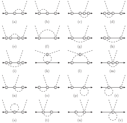
Figure 2: One-loop Feynman diagrams without explicit deltas to order $O(p^{3})$. Dashed and solid lines represent pions and nucleons, respectively. Circled numbers mark the chiral orders of the vertices. Crossed diagrams are not shown.

Figure 3: One-loop Feynman diagrams with explicit deltas to order $O(p^{3})$. Dashed, solid and double lines represent pions, nucleons and deltas, respectively. Circled numbers mark the chiral orders of the vertices. Crossed diagrams, diagrams with the reversed time ordering and diagrams giving vanishing contributions are not shown.

The one-loop Feynman diagrams up to order $\mathcal{O}(p^{3})$, without and with explicit deltas, are shown in Fig. 2 and Fig. 3, respectively. For easier comparison, the labeling scheme for the delta-less loop diagrams of Refs. Alarcon:2012kn ; Chen:2012nx is followed. For the explicit expressions of the contributions of the delta-less one-loop diagrams in the amplitudes we refer the reader to Refs. Alarcon:2012kn ; Chen:2012nx . We have reproduced their results.

Due to the complexity of the spin-$3/2$ delta propagator, the calculation of the delta-full loop diagrams in Fig. 3 is much more complicated. All diagrams have been calculated using two independent computer codes giving identical results. The final expressions are much too huge to be displayed in the paper, however, they can be obtained from the authors.

V Renormalization

To calculate the loop diagrams we apply dimensional regularization with $d$ the number of space-time dimensions. All UV divergences of physical quantities are removed by counter terms generated by the effective Lagrangian and absorbed in the corresponding LECs. The finite pieces of the subtraction terms are fixed such that the subtracted contributions of the loop diagrams in physical quantities satisfy the power counting. The required counter terms are generated by splitting the bare parameters as follows:

$$X \equiv X_{R}+\frac{\bar{\delta}X}{16\pi^{2}F^{2}}R+\frac{\bar{\bar{\delta}}X}{16\pi^{2}F^{2}}\ ,\qquad X\in\{g,h,m,m_{\Delta},a_{1},c_{i=1,\cdot 4}\}\ ,$$ (50)

$$Y \equiv Y_{R}+\frac{\bar{\delta}Y}{16\pi^{2}F^{2}}R\ ,\quad Y\in\{\ell_{3},\ell_{4},d_{1}+d_{2},d_{3},d_{5},d_{14}-d_{15},d_{18}-2d_{16}\}\ ,$$ (51)

where $X_{R}$ and $Y_{R}$ are renormalized parameters and $R\equiv{2}/({d-4})+\gamma_{E}-1-\ln(4\pi)$, and $\gamma_{E}$ is the Euler number.

Below we first introduce the renormalized and physical masses and wave function renormalization constants followed by the definitions of the pion decay constant $F_{\pi}$, the LO $\pi NN$ coupling $g_{\pi N}$ and LO $\pi N\Delta$ coupling $g_{\pi N\Delta}$. In the calculations of $g_{\pi N}$ and $g_{\pi N\Delta}$ we follow a procedure analogous that of Ref. Schindler:2006it . The $\pi N$ scattering amplitudes obtained by using the EOMS scheme are discussed in the end.

V.1 Masses and wave function renormalization constants

V.1.1 Pion

The pions, nucleons and deltas are explicit degrees of freedom in our calculation. Expressions for the pion wave function renormalization constant $\mathcal{Z}_{\pi}$ and the pion pole mass $M_{\pi}^{2}$ at one-loop order have the form (see e.g. Ref. Scherer:2002tk )

$$\mathcal{Z}_{\pi} = 1-\frac{1}{F^{2}}\left[2\ell_{4}M^{2}+\frac{2}{3}\mathcal{H}_{\pi}\right],$$ (52)

$$M_{\pi}^{2} = M^{2}\left[1+\ell_{3}\frac{M^{2}}{F^{2}}-\frac{1}{2F^{2}}\mathcal{H}_{\pi}\right],$$ (53)

where $\mathcal{H}_{\pi}$ is a one-loop integral defined in the appendix together with all loop integrals which contribute in our calculations. Since in dimensional regularization there are no power counting violating terms from the loops, the renormalization of the pion mass can be treated in the standard way of mesonic ChPT by taking $\ell_{3}\equiv\ell_{3R}-\frac{3}{4}\frac{R}{16\pi^{2}}$.

The case of the nucleon is more complicated and can be done in the EOMS scheme so that the PCBTs from loops are dealt properly. We also give the renormalization of the delta mass and the corresponding wave function renormalization constant.

V.1.2 Nucleon

Defining $-i\Sigma_{N}$ as the sum of one-particle irreducible diagrams contributing to the nucleon two-point function, the dressed propagator of the nucleon is given as

$$i\,S_{N}(p)=\frac{i}{\not{p}-m-\Sigma_{N}(\not{p})}=\frac{i\mathcal{Z}_{N}}{\not{p}-m_{N}}+{\rm NP},$$ (54)

where $m_{N}$ is the nucleon pole mass and $\mathcal{Z}_{N}$ is the wave function renormalization constant. NP stands for the non-pole part (also for the delta propagator below).

Figure 4: Tree and one-loop diagrams contributing to the self-energies of the nucleon and the delta resonance up to the order $O(p^{3})$.

The nucleon self-energy up to order ${\cal O}(p^{3})$ consists of tree and loop diagrams shown in Fig. 4 (a), (b) and (c) and the corresponding expressions are given by

$$\Sigma_{N}(\not{p})=-4c_{1}M^{2}+\Sigma_{A}^{N,{\rm loop}}(s)+\not{p}\,\Sigma_{B}^{N,{\rm loop}}(s)\ ,$$ (55)

where $s\equiv p^{2}$ and the first term is the tree-order contribution. The explicit expressions for $\Sigma_{A}^{N,{\rm loop}}(s)$ and $\Sigma_{B}^{N,{\rm loop}}(s)$ are shown in Appendix D. The pole mass of the nucleon, $m_{N}$, corresponding to Eq. (55) is given as the solution to the equation

$$m_{N}=m-4c_{1}M^{2}+\Sigma_{A}^{N,{\rm loop}}(m_{N}^{2})+m_{N}\,\Sigma_{B}^{N,{\rm loop}}(m_{N}^{2})\,.$$ (56)

The nucleon wave function renormalization constant $\mathcal{Z}_{N}$ is given by

$$\mathcal{Z}_{N} = \left[\Sigma_{B}^{N,{\rm loop}}(s)+2s\frac{\partial}{\partial s}\Sigma_{B}^{N,{\rm loop}}(s)+2\not{p}\frac{\partial}{\partial s}\Sigma_{A}^{N,{\rm loop}}(s)\right]_{\not{p}=m_{N}}\,.$$ (57)

Within the on mass-shell renormalization the renormalized mass of a particle is chosen equal to the pole position of the corresponding dressed propagator. In case of BChPT, where we want to keep track of the quark mass dependence of physical quantities explicitly, we use the EOMS scheme Fuchs:2003qc , that is we choose the renormalized mass of the nucleon as the pole mass in the chiral limit. In order to cancel the UV divergence and PCBTs from the loop diagrams, one needs to split the bare parameters $m$ and $c_{1}$ in Eq. (56) as specified by Eq. (50). The explicit expressions of the counter terms ${\bar{\delta}}m$, $\bar{\bar{\delta}}{m}$, ${\bar{\delta}}{c_{1}}$ and $\bar{\bar{\delta}}{c_{1}}$ are given in the Appendix E.

V.1.3 Delta

In case of unstable particles the pole of the dressed propagator is located in the complex plane. We choose the renormalized mass of the delta resonance as the pole position of its dressed propagator in the chiral limit, that is we apply a generalization of the complex-mass scheme introduced originally for the Standard Model Stuart:1990 ; Denner:1999gp . Note that the non-trivial issue of unitarity within the complex-mass scheme has been discussed in Ref. Bauer:2012gn and studied in more details in Ref. Denner:2014zga .

The propagator of the Rarita-Schwinger field corresponding to the Lagrangian of Eq. (27) for $A=-1$ in $d$ space-time dimensions has the form

$$iS_{0,ij}^{\mu\nu}(p) = -\frac{i(\not{p}+m_{\Delta})}{p^{2}-m_{\Delta}^{2}+i0^{+}}\Biggl{[}g^{\mu\nu}-\frac{1}{d-1}\,\gamma^{\mu}\gamma^{\nu}$$ (58)

$$+ \frac{1}{(d-1)m_{\Delta}}(p^{\mu}\gamma^{\nu}-\gamma^{\mu}p^{\nu})-\frac{d-2}{(d-1)m_{\Delta}^{2}}p^{\mu}p^{\nu}\Biggr{]}\xi_{ij}^{\frac{3}{2}}\ .$$

Using notations of Ref. Hacker:2005fh and defining $i\Sigma^{\mu\nu}$ as the sum of one-particle irreducible diagrams contributing to the delta two-point function, we parameterize the self-energy of the $\Delta$ as

$$\Sigma^{\mu\nu} = \Sigma_{1}\,g^{\mu\nu}+\Sigma_{2}\,\gamma^{\mu}\gamma^{\nu}+\Sigma_{3}\,p^{\mu}\gamma^{\nu}+\Sigma_{4}\,\gamma^{\mu}p^{\nu}+\Sigma_{5}\,p^{\mu}p^{\nu}+\Sigma_{6}\,p/\hskip 1.00006ptg^{\mu\nu}$$ (59)

$$+ \Sigma_{7}\,p/\hskip 1.00006pt\gamma^{\mu}\gamma^{\nu}+\Sigma_{8}\,p/\hskip 1.00006ptp^{\mu}\gamma^{\nu}+\Sigma_{9}\,p/\hskip 1.00006pt\gamma^{\mu}p^{\nu}+\Sigma_{10}\,p/\hskip 1.00006ptp^{\mu}p^{\nu},$$

where the $\Sigma_{i}$ are functions of $p^{2}$. The dressed delta propagator has the form

$$i\,S^{\mu\nu}_{ij}(p)=\frac{-i\,g^{\mu\nu}\xi_{ij}^{\frac{3}{2}}}{\not{p}-m_{\Delta}-\Sigma_{1}^{\Delta}(p^{2})-\not{p}\,\Sigma_{6}^{\Delta}(p^{2})}+{\rm NP}=\frac{-i\,g^{\mu\nu}\xi_{ij}^{\frac{3}{2}}\,\mathcal{Z}_{\Delta}}{\not{p}-z_{\Delta}}+{\rm NP},$$ (60)

where the pole position $z_{\Delta}$ of the $\Delta$-propagator is obtained by solving the equation

$$z_{\Delta}-m_{\Delta}-\Sigma_{1}^{\Delta}(z_{\Delta}^{2})-z_{\Delta}\,\Sigma_{6}^{\Delta}(z_{\Delta}^{2})=0\,.$$ (61)

The leading tree-order contribution to the delta self-energy is shown in diagram (d) in Fig. 4 and the leading loop contributions are given by diagrams in Figs. 4 (e) and (f). Similarly to the nucleon case, the delta wave function renormalization constant is obtained via

$$\mathcal{Z}_{\Delta} = \left[\Sigma_{6}^{\Delta,{\rm loop}}(s)+2s\frac{\partial}{\partial s}\Sigma_{6}^{\Delta,{\rm loop}}(s)+2\not{p}\frac{\partial}{\partial s}\Sigma_{1}^{\Delta,{\rm loop}}(s)\right]_{\not{p}=z_{\Delta}}\ .$$ (62)

The explicit expressions of $\Sigma_{1}^{\Delta,{\rm loop}}$ and $\Sigma_{6}^{\Delta,{\rm loop}}$ are given in the Appendix D. Renormalization of the one-loop delta mass is carried out using Eq. (50) with the counter terms shown in Appendix E.

V.2 Coupling constants of the leading order interactions

V.2.1 Pion decay constant $F_{\pi}$

For practical convenience, one often needs to replace the quantities in the chiral limit, $F$, $g_{R}$ and $h_{R}$ by the physical ones, $F_{\pi}$, $g_{\pi N}$ and $g_{\pi N\Delta}$, respectively. At one-loop order the pion decay constant $F_{\pi}$ is given via Gasser:1983yg

$$F_{\pi}=F\left[1+\ell_{4}\frac{M^{2}}{F^{2}}+\frac{1}{F^{2}}\mathcal{H}_{\pi}\right],$$ (63)

which is renormalized in the standard way, i.e. $\ell_{4}=\ell_{4R}-{R}/({16\pi^{2}})$.

V.2.2 Pion-nucleon coupling constant $g_{\pi N}$

Figure 5: Tree and one-loop diagrams contributing to the $g_{\pi N}$ coupling constant up to order $O(p^{3})$.

In the isospin limit $m_{u}=m_{d}=\hat{m}$, where $m_{u}$ and $m_{d}$ are the masses of the $u$ and $d$ quarks, respectively, the matrix element of the pseudoscalar density evaluated between one-nucleon states can be parameterized as

$$\hat{m}\langle N(p^{\prime})|P^{a}(0)|N(p)\rangle=\frac{M_{\pi}^{2}F_{\pi}}{M_{\pi}^{2}-q^{2}}G_{\pi N}(q^{2})\,i\,\bar{u}(p^{\prime})\gamma^{5}\tau^{a}u(p)~{},$$ (64)

where $q=p^{\prime}-p$. $G_{\pi N}(q^{2})$ is called the pion-nucleon form factor and its value at $q^{2}=M_{\pi}^{2}$ defines the pion-nucleon coupling constant $g_{\pi N}=G_{\pi N}(M_{\pi}^{2})$. Tree and one-loop diagrams up to order ${\cal O}(p^{3})$ contributing to the $\pi NN$ vertex function are shown in Fig. 5. The result up to leading one-loop order can be written as

$$g_{\pi N}=\frac{{g}\,m_{N}}{F_{\pi}}(1+g_{\pi N}^{(2)})\ ,\qquad g_{\pi N}^{(2)}=\frac{2(d_{18}-2d_{16})M_{\pi}^{2}}{F_{\pi}^{2}}+g_{\pi N}^{(2),{\rm loop}}\ ,$$ (65)

where $g_{\pi N}^{(2),{\rm loop}}$ represents the very lengthy loop contribution which is not given explicitly in this paper but obtainable from the authors (also the loop contributions to $g_{\pi N\Delta}$ coupling, discussed below). The coupling $g_{\pi N}$ is renormalized in the EOMS scheme and we have checked that the divergences and PCBTs from the loop contributions can indeed be canceled by counter terms generated by ${g}$ and $d_{18}-2d_{16}$.

V.2.3 Pion-nucleon-delta coupling constant $g_{\pi N\Delta}$

Figure 6: Tree and one-loop diagrams contributing to the $g_{\pi N\Delta}$ coupling constant up to order $O(p^{3})$.

Following Ref. Gegelia:2009py we define the “physical” coupling constant $g_{\pi N\Delta}$ by considering the pion-nucleon-delta vertex function $\Gamma$ on the complex mass-shell of the delta. Tree and one-loop diagrams up to order ${\cal O}(p^{3})$ contributing in the $\pi N\Delta$ vertex function are shown in Fig. 6. With $t=q^{2}=(p^{\prime}-p)^{2}$, the form factor $g_{\pi N\Delta}(t)$ is defined by Ellis:1997kc

$$\bar{u}(p^{\prime})\Gamma^{(i,\mu),a}(p,p^{\prime},q)u_{\mu}(p)=g_{\pi N\Delta}(t)\xi^{ia}\bar{u}(p^{\prime})q^{\mu}u_{\mu}(p)~{},$$ (66)

where $u_{\mu}(p)$ and $\bar{u}(p^{\prime})$ are the Dirac spinors of the delta and the nucleon, respectively. We define the ${\pi N\Delta}$ coupling by taking the external pion on the mass-shell, i.e. $g_{\pi N\Delta}=g_{\pi N\Delta}(M_{\pi}^{2})$. One can redefine ${h}$ using Eq. (46) and by that the tree contributions from Diagrams (b) and (c) in Fig. 6 can be absorbed. Hence, the final expression of $g_{\pi N\Delta}$ can be written as

$$g_{\pi N\Delta}=\frac{{h}}{F_{\pi}}(1+g_{\pi N\Delta}^{(2),{\rm loop}})\ ,$$ (67)

with ${h}$ the redefined parameter (as specified in Eq. (46)) and $g_{\pi N\Delta}^{(2),{\rm loop}}$ the loop contribution. Like the renormalization of $g_{\pi N}$, UV-divergences and PCBTs are canceled by counter terms generated by ${h}$. As pointed out e.g. in Ref. Ellis:1997kc , the coupling $g_{\pi N\Delta}$ is a complex-valued quantity.

V.3 The $\pi N$ scattering amplitude

According to the LSZ reduction formula, the $\pi N$ scattering amplitude $T_{\pi N}$ is related to the amputated Greens function $\hat{T}_{\pi N}$, which has been calculated in the above section, via

$$T_{\pi N}=\mathcal{Z}_{\pi}\mathcal{Z}_{N}\bar{u}(p^{\prime})\hat{T}_{\pi N}u(p)\ ,$$ (68)

where $\mathcal{Z}_{\pi}$ and $\mathcal{Z}_{N}$ are the wave function renormalization constants of the pion and the nucleon, respectively.

UV divergences and power counting violating contributions of loop diagrams contributing to the amplitudes which have to be subtracted are calculated by applying the procedure outlined in details in Refs. Fuchs:2003qc ; Schindler:2003xv . We do not give the expressions of these subtraction terms due to their large size. As mentioned above these subtraction terms are canceled by counter terms generated by parameters of the effective Lagrangian, see Eq. (50) and (51). After taking into account the contributions of the counter terms, we obtain a finite amplitude respecting the power counting and possessing the correct analytic behavior.

Note that while we give the explicit form of the counter terms for $c_{1}$ in the appendix, the ones for $c_{2,3,4}$ are too lengthy to be shown here. However, one can display them as

$$c_{i}=c_{iR} + \frac{1}{16\pi^{2}F^{2}}\left\{\mathcal{C}_{1}^{i}\overset{\circ}{\mathcal{H}}_{N}+\mathcal{C}_{2}^{i}\overset{\circ}{\mathcal{H}}_{\Delta}+\mathcal{C}_{3}^{i}\overset{\circ}{\mathcal{H}}_{\pi\Delta}({m}^{2})+\mathcal{C}_{4}^{i}\overset{\circ}{\mathcal{H}}_{\pi N}({m}_{\Delta}^{2})+\mathcal{C}_{5}^{i}\overset{\circ}{\mathcal{H}}_{\pi NN}({m}^{2},0,{m}_{\Delta}^{2})\right.$$ (69)

$$\left.\hskip 42.67912pt+\mathcal{C}_{6}^{i}\overset{\circ}{\mathcal{H}}_{\pi N\Delta}({m}_{\Delta}^{2},0,{m}^{2})+\mathcal{C}_{7}^{i}\overset{\circ}{\mathcal{H}}_{\pi\Delta\Delta}({m}^{2},0,{m}_{\Delta}^{2})\right\},$$

with $i=2,3,4$ and $\mathcal{C}_{j=1,\cdots,7}^{i}$ being the corresponding coefficients. Since the integrals like $\overset{\circ}{\mathcal{H}}_{\pi N}(m_{\Delta}^{2})$ are complex, the $c_{2,3,4}$ are renormalized to complex quantities. Note that $c_{1}$ remains real after renormalization in view of Eq. (108).

Finally, for the sake of practical use, the quantities in the chiral limit contributing to the $\pi N$ amplitude at one-loop order, such as $M$, $m_{R}$, $m_{\Delta R}$, $F$, $g_{R}$ and $h_{R}$, can be substituted by their corresponding physical quantities specified by Eqs. (53), (56), (61), (63), (65) and (67) as this leads to differences beyond the accuracy of the current calculation.

VI Phase shifts and threshold parameters

Based on the $\pi N$ scattering amplitudes specified in the above section, we calculate the phase shifts and threshold parameters. In what follows, we first determine the unknown LECs involved in the $\pi N$ scattering amplitudes by fitting to the phase shifts of the $S$- and $P$-waves. Then we predict the $D$- and $F$-wave phase shifts and the threshold parameters using the determined LECs.

VI.1 Fitting procedure

For the partial wave analysis of the pion-nucleon scattering amplitudes results of several groups are available: Karlsruhe Koch:1980ay ; Koch:1985bn , Matsinos Matsinos:2006sw and GWU SAID . Unfortunately, none of these groups provide uncertainties of their results. Therefore, we prefer to perform fits to the phase shifts generated by the recent Roy-Steiner-equation analysis (RS) of the $\pi N$ scattering Hoferichter:2015hva , where both the central values and the errors of results are given by Schenk-like or conformal parameterizations. Note that this analysis also includes the most up-to-date experimental information on the pion-nucleon scattering lengths. For fitting we extract the RS phase shifts equidistantly from the threshold $W_{\rm th}=1078$ MeV to $W=1318$ MeV with a step-size of $0.8$ MeV. Furthermore, at each fixed energy point, the central value of the phase shift is generated randomly with a normal distribution $N(\mu,\sigma)$, where the mean value $\mu$ and the standard deviation $\sigma$ are specified by the results of the RS equation analysis, and the corresponding error to the central value is assigned to be $\sigma$. This procedure generates a set of simulated data for the chosen energy configuration which is suitable for fitting. In order to obtain stable values for the LECs one should repeat such a procedure as well as fitting for a large number of times, which will generate a large number of (central) values for the LECs and from which the mean values and the statistical errors of the LECs can be determined. In order to achieve this it is enough in our case to repeat the fitting procedure 100 times. Note that our results are Gaussian and thus in fact any procedure using different fitting approaches would lead to the same central values and error bars. Our interest here is to obtain a value of the $\chi^{2}$ which has the usual interpretation, namely a good $\chi^{2}$ corresponds to a value close to 1. For fits done directly using the RS equations a good $\chi^{2}$ would be close to zero.

In the fitting procedure, two $S$-waves, $S_{31}$ and $S_{11}$ and four $P$-waves, $P_{31}$, $P_{11}$, $P_{33}$, $P_{13}$, are taken into account. We use Eq. (16) to extract the phase shifts for $P_{33}$ partial wave, where the Delta resonance is located. For the other partial waves, as discussed in Section II.3, the difference due to various unitarization procedures appears at higher orders, and we use Eq. (19). This is especially advantageous for the $P_{11}$ partial wave, since there is a numerical problem when using Eq. (16) because the real part of the partial wave amplitude vanishes for some energy close to the threshold.

There are eleven LECs (or independent combinations of them) involved in the $\pi N$ amplitudes in total: $c_{1}$, $c_{2}$, $c_{3}$, $c_{4}$, $d_{1}+d_{2}$, $d_{3}$, $d_{5}$, $d_{14}-d_{15}$, $g_{\pi N}$, $g_{\pi N\Delta}$ and $g_{1}$. We fix $g_{\pi N}$ coupling at the central value of $g_{\pi N}^{2}/(4\pi)=13.69\pm 0.20$, which was recently obtained through the Goldberger-Miyazawa-Oehme sum rule Baru:2010xn ; Baru:2011bw . The renormalized couplings $c_{i=1,2,3,4}$ and $g_{\pi N\Delta}$ are complex due to absorption of complex subtraction terms of loop diagrams. Nevertheless, for convenience, we use real-valued renormalized $c_{i}$’s in our fitting procedure and the corresponding imaginary parts of the subtraction terms are retained in the loop contributions rather than absorbed in the $c_{i}$. As for $g_{\pi N\Delta}$, we define

$$h_{A}=g_{\pi N\Delta}F_{\pi}\,,$$ (70)

which is more often used in BChPT and the large-$N_{c}$ relation yields

$$h_{A}=(3g_{A})/2\sqrt{2}\simeq 1.35\ ,\qquad{\rm with}\qquad g_{A}=1.27\ .$$ (71)

Note that our notation differs from the one used in Ref. Pascalutsa:2006up by a factor of 2. Obviously, $h_{A}$ is also a complex coupling in the calculation up to NNLO. However, one can just choose the real part ${\rm Re}[h_{A}]$ as a fitting parameter, and the corresponding imaginary part can be obtained using Eq. (67). In practice, the involved loop integrals can be calculated with all the masses being specified in the next paragraph and hence the imaginary part of $h_{A}$ is given by (up to higher order corrections)

$${\rm Im}[h_{A}]=\frac{\left(1.51F_{\pi}^{2}g_{\pi N}^{2}-1.84{\rm Re}[h_{A}]^{2}\right){\rm Re}[h_{A}]}{160F_{\pi}^{2}\pi^{2}}\ .$$ (72)

Thus we are left with ten unknown real fitting parameters. It is worth noting that $h_{A}$ appearing in the loop contributions can be substituted by ${\rm Re}[h_{A}]$ since the difference caused is of higher order.

For the masses of the particles and the pion decay constant the following values are employed throughout our fitting procedure: $M_{\pi}=139~{}{\rm MeV}$, $m_{N}=939~{}{\rm MeV}$, $z_{\Delta}=(1210-i\,50)~{}{\rm MeV}$, $F_{\pi}=92.2~{}{\rm MeV}$. We take the dimensional regularization scale $\mu=m_{N}$. Here, $z_{\Delta}$ has been identified as the pole position of the dressed delta propagator with its value given by PDG Agashe:2014kda . Note that one can use ${\rm Re}[z_{\Delta}]$ in the loop contributions instead of $z_{\Delta}$ since the difference caused by this approximation is of higher-order, at least order $\mathcal{O}(p^{5})$. This substitution guarantees that all arguments of the required loop integrals are real (no arguments with complex momenta) and, therefore, this enables us to calculate all one-loop integrals using the programs for numerical evaluation OneLoop vanHameren:2010cp and LoopTools Hahn:1998yk . The fits below were performed using the Fortran package MinuitJames:1975dr .

Figure 7: Phase shifts obtained from delta-less BChPT by fitting RS phase shifts in the c.m. energy range $[1082,1110]$ MeV (pion laboratory momentum $q_{\pi}\in[36.1,108.4]$ MeV). Dots with error bars correspond to the RS phase shifts, while circles without error bars stand for the GWU phase shifts. The solid (red) lines represent the results of the current work. The red narrow error bands correspond to the uncertainties propagated from the errors of LECs using Eq. (73). The wide dashed error bands correspond to the theoretical uncertainties due to the truncation of the chiral series estimated by using Eq. (74) proposed in Ref. Epelbaum:2014efa .

Figure 8: Phase shifts obtained from BChPT with explicit delta degrees of freedom in the tree diagrams corresponding to Fit-II. Dots with error bars stand for the RS phase shifts and circles without error bars represent the GWU phase shifts. The solid (red) line represents the result of Fit II of the current work. The red narrow error bands correspond to the uncertainties propagated from the errors of LECs using Eq. (73). The wide dashed error bands correspond to the theoretical uncertainties due to the truncation of the chiral series estimated by using Eq. (74) proposed in Ref. Epelbaum:2014efa .

Figure 9: Phase shifts obtained from BChPT with explicit delta degrees of freedom corresponding to Fit-III. Dots with error bars stand for the RS phase shifts and circles without error bars represent the GWU phase shifts. The solid (red) line represents the result of Fit III of the current work. The red narrow error bands correspond to the uncertainties propagated from the errors of LECs using Eq. (73). The wide dashed error bands correspond to the theoretical uncertainties due to the truncation of the chiral series estimated by using Eq. (74) proposed in Ref. Epelbaum:2014efa .

VI.2 Results

Table 1: Values of the LECs for various fits to the RS phase shifts. The $c_{i}$ and $d_{j}$ are in units of GeV^-1 and GeV^-2, respectively. The statistical and systematic uncertainties are shown in the first and the second brackets, respectively.

	Fit-I	Fit-II	Fit-III
LEC	$N$ (i.e. $\not{\Delta}$)	$N$+LO $\Delta$	$N$+$\Delta$
$c_{1}$	$-1.22(2)(2)$	$-0.99(2)(1)$	$-1.31(2)(1)$
$c_{2}$	$3.58(3)(6)$	$1.38(3)(1)$	$0.78(4)(2)$
$c_{3}$	$-6.04(2)(9)$	$-2.33(3)(1)$	$-2.55(10)(7)$
$c_{4}$	$3.48(1)(3)$	$1.71(2)(1)$	$1.20(4)(2)$
$d_{1+2}$	$3.25(4)(9)$	$0.14(4)(3)$	$4.85(68)(64)$
$d_{3}$	$-2.88(8)(14)$	$-0.97(8)(15)$	$-0.62(10)(15)$
$d_{5}$	$-0.15(6)(14)$	$0.39(6)(11)$	$-0.93(11)(15)$
$d_{14-15}$	$-6.19(7)(12)$	$-1.08(8)(3)$	$5.54(2.79)(2.01)$
$g_{\pi N}$	$13.12^{\ast}$	$13.12^{\ast}$	$13.12^{\ast}$
$h_{A}$	$-$	$1.28(1)(1)$	$1.42(1)(1)-i\,0.16(1)(1)$
$g_{1}$	$-$	$-$	$-1.21(46)(39)$
${{\chi}^{2}}/{\rm dof}$	$\frac{272.0(23.7)}{216-8}=1.31(11)$	$\frac{339.8(27.4)}{328-9}=1.07(9)$	$\frac{373.8(29.9)}{328-10}=1.18(9)$

Table 2: Correlation and covariance coefficients for the fits. The upper and lower triangles correspond to the correlations (in unit of $10^{-2}$) and covariances (in unit of $10^{-4}$), respectively.

Fit-I	$c_{1}$	$c_{2}$	$c_{3}$	$c_{4}$	$d_{1+2}$	$d_{3}$	$d_{5}$	$d_{14-15}$
$c_{1}$	$6$	$83$	$35$	$-10$	$-14$	$-18$	$24$	$16$
$c_{2}$	$7$	$12$	$-22$	$28$	$28$	$-29$	$16$	$-20$
$c_{3}$	$2$	$-2$	$4$	$-62$	$-73$	$19$	$13$	$65$
$c_{4}$	$1$	$1$	$-2$	$2$	$26$	$-8$	$-4$	$-19$
$d_{1+2}$	$-1$	$4$	$-6$	$1$	$14$	$-4$	$-37$	$-77$
$d_{3}$	$-3$	$-8$	$3$	$-1$	$-1$	$65$	$-91$	$27$
$d_{5}$	$3$	$3$	$2$	$1$	$-8$	$-42$	$32$	$6$
$d_{14-15}$	$3$	$-5$	$10$	$-2$	$-21$	$15$	$3$	$51$

Fit-II	$c_{1}$	$c_{2}$	$c_{3}$	$c_{4}$	$d_{1+2}$	$d_{3}$	$d_{5}$	$d_{14-15}$	${\rm Re}[h_{A}]$
$c_{1}$	$6$	$80$	$36$	$-16$	$-17$	$-17$	$25$	$19$	$17$
$c_{2}$	$6$	$12$	$-26$	$31$	$31$	$-28$	$14$	$-25$	$-27$
$c_{3}$	$2$	$-2$	$7$	$-72$	$-78$	$18$	$17$	$74$	$80$
$c_{4}$	$-1$	$2$	$-3$	$2$	$42$	$-10$	$-10$	$-38$	$-56$
$d_{1+2}$	$-2$	$4$	$-9$	$3$	$16$	$-3$	$-39$	$-80$	$-64$
$d_{3}$	$-3$	$-8$	$4$	$-1$	$-1$	$64$	$-90$	$25$	$18$
$d_{5}$	$3$	$3$	$3$	$-1$	$-9$	$-41$	$33$	$10$	$11$
$d_{14-15}$	$3$	$-7$	$16$	$-5$	$-25$	$16$	$4$	$60$	$63$
${\rm Re}[h_{A}]$	$1$	$1$	$1$	$1$	$-1$	$1$	$1$	$2$	$1$

Fit-III	$c_{1}$	$c_{2}$	$c_{3}$	$c_{4}$	$d_{1+2}$	$d_{3}$	$d_{5}$	$d_{14-15}$	${\rm Re}[h_{A}]$	$g_{1}$
$c_{1}$	$6$	$67$	$-7$	$7$	$18$	$-8$	$-4$	$-16$	$5$	$-18$
$c_{2}$	$7$	$19$	$-44$	$56$	$27$	$-20$	$-7$	$18$	$-61$	$-25$
$c_{3}$	$-2$	$-19$	$91$	$-93$	$-86$	$-37$	$68$	$-88$	$51$	$91$
$c_{4}$	$1$	$9$	$-33$	$14$	$73$	$26$	$-55$	$72$	$-64$	$-77$
$d_{1+2}$	$30$	$80$	$-562$	$186$	$4650$	$44$	$-85$	$87$	$-11$	$-97$
$d_{3}$	$-2$	$-8$	$-34$	$9$	$284$	$90$	$-79$	$55$	$15$	$-50$
$d_{5}$	$-1$	$-3$	$68$	$-22$	$-609$	$-79$	$110$	$-73$	$-3$	$81$
$d_{14-15}$	$105$	$213$	$-2339$	$752$	$16597$	$1456$	$-2142$	$77827$	$-11$	$-97$
${\rm Re}[h_{A}]$	$1$	$-1$	$2$	$-1$	$-4$	$1$	$1$	$-16$	$1$	$15$
$g_{1}$	$-19$	$-50$	$403$	$-133$	$-3053$	$-219$	$393$	$-12474$	$4$	$2142$

The fitted LECs for three different cases are given in Table 1, where the statistical and systematic uncertainties are shown in the first and second brackets behind the central values, respectively. The systematic uncertainties represent the effects of varying the fitting ranges, which will be discussed later on in this section. The covariance and correlation matrices between the LECs are given in Table 2. They are calculated using the standard formulae

$${\rm Cor}(x_{i},x_{j}) = \frac{{\rm Cov}(i,j)}{\sqrt{{\rm Cov}(x_{i},x_{i}){\rm Cov}(x_{j},x_{j})}}\ ,$$

$${\rm Cov}(x_{i},x_{j}) = \frac{(\bf{x_{i}}-\bar{\bf{x_{i}}})^{T}\cdot(\bf{x_{j}}-\bar{\bf{x_{j}}})}{N-1}\ ,$$

where ${\bf x_{i}}$ is the vector of $N$ central values of the LECs obtained from the fitting of our pseudo-data as explained before, for our case $N=100$. There are strong correlations between some LECs. Results of our fits are displayed and compared with the phase shifts of the RS analysis as well as GWU analysis in Figures 7, 8 and 9. The red narrow bands stand for the uncertainties propagated from the errors of the LECs using

$$\delta\,\mathcal{O}_{\rm LEC}=\bigg{\{}\left[\frac{\partial\mathcal{O}(\bar{x}_{i})}{\partial x_{i}}\right]^{2}\left(\delta x_{i}\right)^{2}+{\rm Cor}(x_{i},x_{j})\left[\frac{\partial\mathcal{O}(\bar{x}_{i})}{\partial x_{i}}\right]\left[\frac{\partial\mathcal{O}(\bar{x}_{j})}{\partial x_{j}}\right]\delta x_{i}\delta x_{j}\bigg{\}}^{\frac{1}{2}}\,,\ i\neq j\,,$$ (73)

where $\mathcal{O}$ is any observables under consideration and the summation over the repeated indices is meant. Note that the contributions from statistical and systematic errors of the LECs to the error of the observable $\mathcal{O}$ are added in quadrature. The dashed wide bands represent uncertainties estimated by truncation of the chiral series for the central values of LECs, using the method which was proposed in Ref. Epelbaum:2014efa . To be specific, the uncertainty $\delta\,\mathcal{O}^{(n)}$ of a prediction for an observable $\mathcal{O}$ up to $O(p^{n})$ is assigned to be

$$\delta\,\mathcal{O}^{(n)}_{\rm theo.}={\rm max}\big{(}|\mathcal{O}^{(n_{\rm LO})}|Q^{n-n_{\rm LO}+1},\{|\mathcal{O}^{(k)}-\mathcal{O}^{(j)}|Q^{n-j}\}\big{)}\,,\qquad n_{\rm LO}\leq j<k\leq n\,,$$ (74)

with $Q=\omega_{q}/\Lambda_{b}$ where $\omega_{q}$ and $\Lambda_{b}$ are the pion energy in the center-of-mass frame and the breakdown scale of the chiral expansion, respectively. For the delta-full case, we choose to employ $\Lambda_{b}\sim 0.6$ GeV following Ref. Epelbaum:2014efa , which is lower than the scale of the chiral symmetry breaking $\Lambda_{\chi}\sim 4\pi F_{\pi}\sim 1$ GeV. The lightest particle we do not include explicitly is the Roper resonance $N^{*}(1440)$ and its mass differs from the nucleon mass by about $0.5$ GeV. Our choice of $\Lambda_{b}$ is close to that number. Similarly, for the delta-less case, $\Lambda_{b}$ is taken $0.4$ GeV due to the nucleon-delta mass difference. For more discussions on the choice of $\Lambda_{b}$ see Ref. Siemens:2016hdi . Now let us proceed with the details of the three different fits.

Fit-I corresponds to the delta-less case and is performed up to $W_{\rm max}$=$1.11$ GeV. This maximal energy is chosen according to the following criterions: I) the average $\overline{\chi^{2}}$ per degree of freedom ($\overline{\chi^{2}}/{\rm d.o.f}$) for the 100-times fits is around $1.0,$ II) the average $\overline{\chi^{2}}$ increases rapidly if one takes larger $W_{\rm max}$. For Fit-I, we get results similar to those obtained by fitting to the phase shifts of partial wave analysis by GWU group up to $1.13$ GeV Alarcon:2012kn ; Chen:2012nx . There exist slight differences between our current results and the previous ones Alarcon:2012kn ; Chen:2012nx due to the fact that different data (RS data versus GWU data) were fitted and the fitting ranges are not the same. Besides, they have one more fitting parameter $d_{18}$, which is related to $g_{\pi N}$ by making use of the Goldberber-Treiman relation at NNLO. Our plots for Fit-I are shown in Figure 7. The error bands in $P_{33}$ and $S_{31}$ partial waves do not cover the RS and GWU data beyond the fitting range, which suggests that $\Lambda_{b}=0.4$ GeV underestimates the theoretical errors for these partial waves.

Adding the delta degree of freedom should mostly improve the description of the $P_{33}$ wave in the $\Delta$-resonance region. We thus performed two fits (Fit-II and Fit-III) using 1.2 GeV as $W_{\rm max}$ for the $P_{33}$ partial wave and 1.11 GeV for the other five partial waves - the same value as for Fit I. Fit II is done by adding the LO Born-term contribution of the delta-exchange diagrams to the delta-less case and serves only the purpose of estimating the effect of the loop diagrams. Our plots for Fit-II are shown in Figure 8. Since only the tree order contributions of the delta are included, $h_{A}$ is a real parameter and meanwhile $g_{1}$ does not show up in Fit-II. Compared to the strategies in Refs. Alarcon:2012kn ; Chen:2012nx , in the current work the complex pole position of the delta propagator rather than the real mass is incorporated in a systematic way and hence the effect of the delta width is included explicitly. We obtain better results with smaller uncertainties than the previous studies, for instance, the large errors in $d_{14}-d_{15}$ are substantially reduced.

Fit-III is done (up to 1.2 GeV for $P_{33}$ and up to $1.11$ GeV for the other waves) with the full contributions of pions, nucleons and deltas up to NNLO. The obtained LECs of Fit-III are different from those of Fit-II due to the inclusion of contributions of loop diagrams involving delta lines. Note that all the $c_{i}$ and most of the higher order LECs are of natural size. Our plots for Fit-III are shown in Figure 9. Compared to the plots in Figure 8, although both fits describe well the phase shifts in the fitting range, Fit-III improves the predictions beyond fitting ranges in most of the partial waves, especially for the $S_{11}$ wave. The larger theoretical error in Figure 9 compared to Figure 8 is due to the large contributions of delta-loop diagrams, which are not taken into account in estimation of the theoretical error of Fit-II using Eq. (74).

As one can see from Table 1, the imaginary part of $h_{A}$ from Fit-III is small compared to the corresponding real part ${\rm Re}[h_{A}]$ and our determination for ${\rm Re}[h_{A}]$ is close to the large-$N_{c}$ prediction (71). The obtained $g_{1}$ for Fit-III is nearly consistent (within the error bars) with the corresponding large-$N_{C}$ result, $|g_{1}|=9g_{A}/5\simeq 2.28$. As noted in Ref. Fettes:2000bb , $g_{1}$ appears only in the loop contribution, hence a precise determination of its value is not to be expected.

All the above three fits are done with their own preferred $W_{\rm max}$. However, following Ref. Durr:2014oba , one can change those maximal energies around the preferred $W_{\rm max}$ and redo the fits to see the influence on the obtained LECs. For Fit-I, we made fits with $W_{\rm max}=1.11\pm 0.004$ GeV, $1.11\pm 0.008$ GeV, $1.11\pm 0.012$ GeV and $1.11\pm 0.016$ GeV in order to produce such kind of systematic errors to the LECs. For Fit-II and Fit-III, we keep the maximal energy at $1.2$ GeV for the $P_{33}$ partial wave but vary it for the other waves as is the case for Fit-I. A demonstration of how to obtain the systematic errors is given in Fig. 10 for the case of Fit-I and analogous figures are obtained for other three fits. The obtained systematic errors to the LECs are shown in the second bracket in Table 1.

Note that all the presented fits have been done with the energy steps of $0.8$ MeV. We have checked that the influence of varying the energy step on the central values of the LECs is essentially negligible. Also the statistical errors decrease when the fitting range is extended keeping the energy step the same, see Fig. 10, or more fitting points are added in the same fitting range. However, we do not estimate such systematic uncertainties here.

Using the LECs obtained by fitting to the phase shifts of $S$- and $P$-waves, one can predict the phase shifts of higher partial waves. In Fig. 11 we show the phase shifts of $D$ and $F$ partial waves obtained using the parameters of Fit-I and Fit-III compared to the results obtained by the GWU group  SAID . As expected, the predicted phase shifts of higher partial waves are indeed small. Except for $D_{33}$ channel, our predictions agree qualitatively with the GWU results and the predictions of the delta-full theory are somewhat better than those of the delta-less theory.

Figure 10: Demonstration of the effect of varying the fitting range on the fitted LECs. The solid (blue) line with inner (cyan) band indicate the central value and the statistical error which come from the preferred fit with $W_{\rm max}=1.11$ GeV. The outer (blue) band is yielded by adding the systematic uncertainty which is generated by the scatter of all results with different fitting ranges. The error bars correspond to statistical errors of the fitting procedure.

Figure 11: Phase shifts of the $D$ and $F$ partial waves obtained from the delta-less and delta-full BChPT using the parameters of Fit-I (red line extending up to 1.16 GeV) and Fit-III (blue line with band extending up to 1.2 GeV), respectively. The circles correspond to phase shifts by the GWU group  SAID .

Finally, in order to demonstrate how well Eq. (16) extracts phase shifts from perturbative amplitudes, we draw the so-called Argand plot for the $P_{33}$ partial wave in Fig. 12 by using the LECs of Fit-III. In Fig. 12 the red solid and the magenta dashed lines correspond, respectively, to the full contribution ($\pi$+$N$+$\Delta$) and the contribution of the pion and nucleon ($\pi+N$) alone. As we can see, the inclusion of the $\Delta$ contribution has a huge influence on improving the unitarity constraints. The unitarized amplitude based on the full contribution is represented by the blue dotted line, which is located on the unitary circle (broad cyan solid circle), as expected. The energy corresponding to the 15th point is $W_{15}=1314$ MeV and the interval between two adjacent points on the same line is $16$ MeV. The effect of Eq. (16) is to move the points of the full NNLO perturbative amplitudes to the closest positions on the unitary circle.

Figure 12: Argand diagram for the $P_{33}$ partial wave for the LECs of Fit-III. For a detailed description see the text.

VI.3 Scattering lengths and volumes

At low energies, one can predict the threshold parameters based on the above determined LECs. For the partial wave with angular momentum $\ell$ the general form of the effective range expansion is given by

$$|{\bf p}|^{2\ell+1}{\rm cot}[\delta_{\ell\pm}^{I}]=\frac{1}{a_{\ell\pm}^{I}}+\frac{1}{2}r_{\ell\pm}^{I}|{\bf p}|^{2}+\sum_{n=2}^{\infty}v_{n,\ell\pm}^{I}|{\bf p}|^{2n}\,,$$ (75)

where ${\bf p}$ is the three-momentum of the nucleon in CMS frame, $a$ is the threshold parameter (e.g. scattering length for the $S$-wave and scattering volume for the $P$-wave), $r$ is the effective range parameter, and $v_{n}$ are the shape parameters. Using Eq. (75) one can obtain the threshold parameters as

$$a_{\ell\pm}^{I}=\lim_{|{\bf p}|\to 0}\frac{\tan\delta_{\ell\pm}^{I}}{|{\bf p}|^{2\ell+1}}=\lim_{|{\bf p}|\to 0}\frac{{\rm Re}f_{\ell\pm}^{I}(s)}{|{\bf p}|^{2\ell}}\,.$$ (76)

The second equality holds true due to the fact that the imaginary parts of the partial wave amplitudes vanish faster at threshold. As ${{\rm Re}f_{\ell\pm}^{I}(s)}/{|{\bf p}|^{2\ell}}$ can not be computed numerically exactly at the threshold we calculated its values for energies very close to the threshold and then obtained the threshold parameters by extrapolating to the threshold. Results of the threshold parameters corresponding to the three different fits are presented in Table 3, together with the determinations from the Roy-Steiner equation analysis Hoferichter:2015hva (and the input from the analysis of pionic hydrogen and deuterium atom data). The errors in the first brackets are propagated from the uncertainties of the LECs, while the ones in the second brackets are obtained via Eq. (74). After taking the errors into consideration, all the obtained results agree well with those of the Roy-Steiner equation analysis, especially for Fit-III.

Table 3: Scattering lengths and volumes. The numbers in brackets correspond to the errors propagated from the uncertainties of LECs and the theoretical errors, respectively.

Threshold Para.	Fit-I	Fit-II	Fit-III	RS Hoferichter:2015hva
$a_{0+}^{+}~{}[10^{-3}M_{\pi}^{-1}]$	$-0.6(7)(3.4)$	$-1.1(7)(3.0)$	$-0.5(7)(7.1)$	$-0.9(1.4)$
$a_{0+}^{-}~{}[10^{-3}M_{\pi}^{-1}]$	$85.7(5)(3.3)$	$85.8(4)(1.1)$	$85.8(3)(1.0)$	$85.4(9)$
$a_{1-}^{+}~{}[10^{-3}M_{\pi}^{-3}]$	$-49.8(1.0)(15.9)$	$-52.5(4)(4.7)$	$-51.0(5)(6.7)$	$-50.9(1.9)$
$a_{1-}^{-}~{}[10^{-3}M_{\pi}^{-3}]$	$-9.7(3)(9.5)$	$-11.3(3)(3.2)$	$-9.5(2)(1.7)$	$-9.9(1.2)$
$a_{1+}^{+}~{}[10^{-3}M_{\pi}^{-3}]$	$139.9(1.8)(11.6)$	$131.0(4)(4.0)$	$131.5(5)(8.8)$	$131.2(1.7)$
$a_{1+}^{-}~{}[10^{-3}M_{\pi}^{-3}]$	$-84.0(6)(4.0)$	$-80.3(1)(1.4)$	$-80.4(2)(2.3)$	$-80.3(1.1)$

VII Baryon sigma terms and the strangeness content of the nucleon

Sigma terms are interesting observables and important for understanding the sea-quark structures of baryons. In particular, for the nucleon there are many studies of the $\pi N$ $\sigma$-term, e.g., see Refs. Bernard:1993nj ; Alarcon:2011zs ; Hoferichter:2015dsa , and of the strangeness content, see Refs. Gasser:1980sb ; Borasoy:1996bx ; Alarcon:2012nr ; Ren:2014vea for instance. A high-precision determination of the $\sigma_{\pi N}$ was done from RS-equation analysis based on the improved Cheng-Dashen low-energy theorem and $\sigma_{\pi N}=(59.1\pm 3.5)$ MeV was reported in Ref. Hoferichter:2015dsa . In this section we discuss the $\sigma_{\pi N}$ based on our fitted results obtained above. In order to estimate the strangeness content of the nucleon, we perform the corresponding calculation in SU(3) BChPT. As byproducts, the baryon sigma terms are also given.

VII.1 $\pi N$ sigma term

The $\pi N$ sigma term $\sigma_{\pi N}$ can be obtained from the nucleon mass by applying the Hellmann-Feynman theorem,

$$\sigma_{\pi N}=\hat{m}\frac{\partial m_{N}}{\partial\hat{m}},\quad\hat{m}=\frac{(m_{u}+m_{d})}{2}\ .$$ (77)

For practical convenience, using the expression of the nucleon mass $m_{N}$ given in Section V.1.2, one can express $\sigma_{\pi N}$ as

$$\sigma_{\pi N}=\underbrace{-77.28\,c_{1}}_{\rm LO}+\underbrace{(-11.72)\,g_{A}^{2}+(-6.55)\,{\rm Re}[h_{A}]^{2}}_{\rm NLO}\ ,$$ (78)

where the involved loop integrals have been computed numerically. Notice that the last term in this expression does not contribute in the calculation of the sigma terms of Fit-I and Fit-II.

The results for the pion-nucleon sigma term $\sigma_{\pi N}$ based on the different fitting results in the above section are shown in Table 4, where contributions from different orders are also shown. The error in the first bracket is propagated from the uncertainties of the fitted LECs using Eq. (73). The error in the second bracket is theoretical uncertainty estimated using Eq. (74) and we employ $Q=M_{\pi}/\Lambda_{b}$ with $\Lambda_{b}=400$ MeV for the delta-less case and with $\Lambda_{b}=600$ MeV for the delta-full case. Note that here for Fit-II the theoretical error originating from the delta-loop contribution is also taken into account. For easy comparison, the recent determination of the pion-nucleon sigma term from the Roy-Steiner equations Hoferichter:2015dsa is also given.

Our prediction for Fit-I, $\sigma_{\pi N}=74.8(2.2)(11.4)$ MeV, is marginally consistent with the RS determination when the large uncertainties are taken into account. For the delta-full case with LO delta contribution, applying the same unitarization as in Ref. Alarcon:2011zs , we obtain $\sigma_{\pi N}=60.1(1.6)(6.2)$ MeV based on Fit-II. On the other hand, by including the explicit delta width rather than generating it by unitarization as in Ref. Alarcon:2011zs , we obtained $\sigma_{\pi N}=57.1(1.9)(7.0)$ MeV based on Fit-II, which appears to agree with the RS determination very well. As for Fit-III, our prediction $\sigma_{\pi N}=68.5(1.9)(7.6)$ MeV improves the delta-less result and within the error it overlaps the value of the RS analysis. The large estimated theoretical error comes from the delta-loop diagram contributions by using Eq. (74).

Table 4: The pion-nucleon sigma term in units of MeV. The numbers in brackets correspond to the errors propagated from the uncertainties of LECs and the theoretical errors, respectively.

	Fit-I	Fit-II	Fit-III	RS Hoferichter:2015dsa
LO	$94.3$	$76.5$	$101.2$	$-$
NLO	$-19.5$	$-19.5$	$-32.7$	$-$
Sum	$74.8(2.2)(11.4)$	$57.1(1.9)(7.0)$	$68.5(1.9)(7.6)$	$59.1(3.5)$

VII.2 The strangeness content of the nucleon and the sigma terms of baryons from SU(3) BChPT

Similarly to $\sigma_{\pi N}$ one can obtain the nucleon expectation value of the operator $m_{s}\bar{s}s$ using the Hellmann-Feynman theorem,

$$\sigma_{sN}=m_{s}\frac{\partial m_{N}}{\partial m_{s}}\ ,$$ (79)

where $m_{s}$ is the mass of the strange quark. However, the nucleon mass $m_{N}$ in the above equation should be calculated in SU(3) BChPT. We calculated the masses of the baryon octet in SU(3) BChPT also including the baryon decuplet as explicit degrees of freedom up to third order. Details of this calculation are specified in the Appendix F. The other baryon sigma terms are also obtainable by using formulas similar to Eqs. (77) and  (79) but with the nucleon mass being replaced by $m_{\Sigma}$, $m_{\Lambda}$ or $m_{\Xi}$.

The strangeness content of the nucleon $y$ is defined through

$$y=\frac{2\hat{m}}{m_{s}}\frac{\sigma_{sN}}{\sigma_{\pi N}},$$ (80)

and the nucleon expectation value of the operator $\bar{u}u+\bar{d}d-2\bar{s}s$ (see e.g. Borasoy:1996bx ) is given by the following equation

$$\sigma_{0}={\sigma_{\pi N}}{(1-y)}.$$ (81)

In order to determine the strangeness content of the nucleon and the sigma terms specified above, we first need to pin down the unknown LECs involved in the SU(3) calculation. Therefore, we fit to the experimental values for $m_{N}$, $m_{\Sigma}$, $m_{\Lambda}$ and $m_{\Xi}$ (taken from PDG Agashe:2014kda ) as well as the RS determination of $\sigma_{\pi N}$, as given in the last column of Table 4. There are the following five unknown LECs: the octet mass in the chiral limit $M_{0}$, the LECs corresponding to the NLO mass splitting operators $b_{0}$, $b_{D}$ and $b_{F}$, and the LO Goldstone-boson-octet-decuplet coupling constant $\mathscr{C}$. For the other parameters we use the following values

$$D = 0.80,\quad F=0.46,\quad M_{\pi}=0.139~{}{\rm GeV},\quad M_{K}=0.494~{}{\rm GeV},$$

$$M_{B} = 1.151~{}{\rm GeV},\quad M_{D}=1.382~{}{\rm GeV},$$ (82)

with $M_{B}$ and $M_{D}$ being the averages of the physical masses of the octet and decuplet, respectively. The mass of the $\eta$ meson is obtained from the Gell-Mann-Okubo relation: $3M_{\eta}^{2}=4M_{K}^{2}-M_{\pi}^{2}$. Furthermore, $F_{\phi}=1.17F_{\pi}$ with $F_{\pi}=92.2$ MeV is used.

We performed two fits:

• Fit A: The octet baryon mass in the loops is fixed at $M_{B}$, and the mass of the decuplet baryons to $m_{D}$.

• Fit B: The octet baryon mass in the loops is set as the chiral limit mass $M_{0}$, and the mass of the decuplet baryons to $m_{D}$.

If the chiral series of the baryon masses and the sigma terms converges well, these two fits should differ slightly since the differences are of high order. However, we obtain results with sizable differences (see $y$ and $\sigma_{0}$ together with the fitted parameters in Table 5) which implies that the higher-order contributions are large. Only when the theoretical errors, which is due to the truncation of the chiral series using Eq. (74) with $Q=M_{\pi}/\Lambda_{\chi}$, are taken into account, these fit results overlap. The previous determinations are as follows: $y=0.15(10)$ and $\sigma_{0}=33(5)$ of the NLO calculation Gasser:1980sb , $y=0.21(20)$ and $\sigma_{0}=36(7)$ of the NNLO calculation within HBChPT Borasoy:1996bx , $y=0.02(23)$ and $\sigma_{0}=58(8)$ of the NNLO calculation within Covariant BChPT Alarcon:2012nr . We therefore conclude that to this order in the chiral expansion, one is not able to make a precise statement about the strangeness content of the nucleon. Likewise, various values of $y$ calculated either directly in Lattice QCD, or indirectly using the octet baryon masses and sigma terms obtained in Lattice QCD, are very different. Therefore we do not compare to those results.

We also predict the octet baryon masses and sigma terms in Table 6 and Table 7, respectively. The errors for the masses and the ones in the first brackets for the sigma terms are propagated from the uncertainties of the LECs. For the sigma terms we also estimated the theoretical errors, which are shown in the second brackets in Table 7. As we can see, the theoretical errors for $\sigma_{sN}$ are very large due to the bad convergence of the chiral series in SU(3) BChPT. Note also that determinations of $\sigma_{sN}$ by different Lattice QCD collaborations vary in a large range, see e.g. Refs Durr:2011mp ; Yang:2015uis ; Durr:2015dna ; Horsley:2011wr ; Freeman:2012ry ; Junnarkar:2013ac ; Oksuzian:2012rzb ; Engelhardt:2012gd ; Gong:2013vja ; Abdel-Rehim:2016won .

Table 5: LECs and strangeness content of the nucleon. Results are obtained with $z=-1$ and $\mu=1$ GeV. The numbers in brackets for $y$ and $\sigma_{0}$ correspond to the errors propagated from the uncertainties of LECs and the theoretical errors, respectively.

	$M_{0}~{}({\rm GeV})$	$b_{0}$	$b_{D}$	$b_{F}$	$\mathscr{C}$	$y~{}~{}[\%]$	$\sigma_{0}~{}~{}[{\rm MeV}]$
Fit-A	$0.654(1)$	$-1.155(1)$	$0.122(1)$	$-0.359(1)$	$1.495(5)$	$1.2(6)(12.1)$	$58.4(4)(9.0)$
Fit-B	$0.622(2)$	$-0.956(1)$	$0.082(1)$	$-0.368(1)$	$2.289(20)$	$20.2(6)(6.5)$	$47.2(4)(5.2)$

Table 6: Masses of octet baryons obtained with the LECs given in Table 5. The numbers in brackets correspond to the errors propagated from the uncertainties of LECs and the theoretical errors, respectively.

	$m_{N}$	$m_{\Lambda}$	$m_{\Sigma}$	$m_{\Xi}$
Fit-A	$939.2(5.0)(61.8)$	$1115.7(4.5)(77.1)$	$1186.0(4.5)(87.7)$	$1327.4(4.3)(97.6)$
Fit-B	$939.2(6.1)(33.7)$	$1115.7(5.6)(51.7)$	$1186.0(5.5)(55.6)$	$1327.4(5.4)(71.7)$
expt.	$938.925(645)$	$1115.683(6)$	$1193.15(4.30)$	$1318.28(3.43)$

Table 7: Sigma terms obtained with the LECs given in Table 5. The numbers in brackets correspond to the errors propagated from the uncertainties of LECs and the theoretical errors, respectively.

	Fit-A	Fit-B
$\sigma_{\pi N}$	$59.1(2)(5.5)$	$59.1(2)(3.6)$
$\sigma_{\pi\Lambda}$	$46.9(2)(5.5)$	$45.8(2)(3.6)$
$\sigma_{\pi\Sigma}$	$38.6(2)(5.7)$	$40.7(2)(3.7)$
$\sigma_{\pi\Xi}$	$30.5(2)(5.6)$	$30.0(2)(3.7)$
$\sigma_{sN}$	$8.5(4.4)(86.6)$	$144.7(4.6)(45.9)$
$\sigma_{s\Lambda}$	$166.0(3.7)(106.3)$	$297.2(3.8)(69.1)$
$\sigma_{s\Sigma}$	$203.6(3.9)(122.3)$	$355.4(4.0)(75.2)$
$\sigma_{s\Xi}$	$342.5(3.4)(133.9)$	$479.0(3.4)(95.3)$

VIII Summary and conclusion

In this paper we presented the ${\cal O}(p^{3})$ order calculation of the pion-nucleon scattering amplitudes in the framework of BChPT including pions, nucleons and deltas as explicit degrees of freedom. There are tree and one-loop diagrams contributing at this order. We applied the EOMS renormalization scheme to loop diagrams involving pion and nucleon lines only. For diagrams with the delta lines in loops we used the complex-mass scheme which is a generalization of the on-mass-shell scheme for unstable particles. That is we subtracted the divergent pieces and the power counting violating contributions of the loop diagrams by canceling them by counter terms generated by splitting the bare parameters of the effective Lagrangian in renormalized couplings and counter terms.

We fitted the renormalized coupling constants to the $S$- and $P$-wave phase shifts, which are randomly generated by using the results of the Roy-Steiner equation analysis of Ref. Hoferichter:2015hva and hence are normally distributed simulations. Both the phase shifts extracted from the RS equation analysis and the GWU group analysis SAID are well described up to 1.11 GeV for the delta-less case. For the delta-full case, the $P_{33}$ partial wave is fitted up to 1.20 GeV while the other partial waves up to 1.11 GeV.

Based on the obtained LECs, we predicted the $D$- and $F$-wave phase shifts and compared them with the results given by the GWU group. We found that our prediction for $D_{33}$ wave differs from the determination of the GWU group while the predictions for other $D$ and $F$ waves agree well. Considering the Argand plot for the $P_{33}$ partial wave we checked that the unitarized amplitude, from which we extracted the phase shifts, is a good approximation to the amplitude obtained by our perturbative calculation. At low energies, we extracted the threshold parameters and compared to the corresponding results of the Roy-Steiner equation analysis obtaining satisfactory agreement.

In addition, we calculated the pion-nucleon sigma term. Our extractions of $\sigma_{\pi N}$ based on the fitted LECs of Fit-I and Fit-III are consistent with the result of RS analysis $\sigma_{\pi N}=(59.1\pm 3.5)$ MeV taking into account the large errors of our determination.

In the end, we also studied the strangeness content of the nucleon $y$ in SU(3) BChPT. We first fixed all the involved SU(3) LECs by fitting to the experimental octet baryon masses as well as the RS result $\sigma_{\pi N}=(59.1\pm 3.5)$ MeV Hoferichter:2015dsa . Two different strategies were used. In principle, they should only slightly differ from each other since the differences are due to higher-order contributions. However, because of the bad convergence properties of the SU(3) BChPT for these quantities, we obtained two sets of predictions with rather large discrepancies from each other. Nevertheless, when the large uncertainties are taken into account, they are consistent with each other. Hence at the order one is working here, we unfortunately cannot disentangle a small from a large value of $y$. Similar picture appears when one takes an overall view on the previous determinations from BChPT Gasser:1980sb ; Borasoy:1996bx ; Alarcon:2012nr and Lattice QCD Durr:2011mp ; Yang:2015uis ; Durr:2015dna ; Horsley:2011wr ; Freeman:2012ry ; Junnarkar:2013ac ; Oksuzian:2012rzb ; Engelhardt:2012gd ; Gong:2013vja ; Abdel-Rehim:2016won ; Bali:2016lvx . Within these two strategies, we predict all the octet baryon sigma terms as well.

Appendix A Tree amplitudes of delta-exchange

In what follows, the amplitudes corresponding to tree-order delta-exchange diagrams are given explicitly here.

• Born-terms of $\mathcal{O}(p^{1})$ diagram (g):

  $$A^{+}_{g}(s,t) = \frac{h^{2}}{9F^{2}{m}_{\Delta}^{3}({m}_{\Delta}^{2}-s)}{\mathcal{F}_{A}(s,t)},\qquad A^{-}_{g}(s,t)=-\frac{1}{2}A^{+}_{g}(s,t),$$

  $$B^{+}_{g}(s,t) = -\frac{h^{2}}{9F^{2}{m}_{\Delta}^{3}({m}_{\Delta}^{2}-s)}{\mathcal{F}_{B}(s,t)},\qquad B^{-}_{g}(s,t)=-\frac{1}{2}B^{+}_{g}(s,t).$$ (83)

• Born-terms of $\mathcal{O}(p^{2})$ diagrams (h+i):

  $$A^{+}_{hi}(s,t) = \frac{2h}{9F^{2}{m}_{\Delta}^{3}({m}_{\Delta}^{2}-s)}\left\{b_{3}\,\mathcal{G}_{A}(s,t)+b_{8}\frac{(s-m_{N}^{2}-M_{\pi}^{2})}{2m_{N}}\mathcal{F}_{A}(s,t)\right\},$$

  $$B^{+}_{hi}(s,t) = -\frac{2h}{9F^{2}{m}_{\Delta}^{3}({m}_{\Delta}^{2}-s)}\left\{b_{3}\,\mathcal{G}_{B}(s,t)+b_{8}\frac{(s-m_{N}^{2}-M_{\pi}^{2})}{2m_{N}}\mathcal{F}_{B}(s,t)\right\},$$

  $$A^{-}_{hi}(s,t) = -\frac{1}{2}A^{+}_{hi}(s,t),\qquad B^{-}_{hi}(s,t)=-\frac{1}{2}B^{+}_{hi}(s,t).$$ (84)

• Born-terms of $\mathcal{O}(p^{3})$ diagrams (j+k):

  $$A^{+}_{jk}(s,t) = \frac{2h}{9F^{2}{m}_{\Delta}^{3}({m}_{\Delta}^{2}-s)}\left\{-f_{1}\frac{s-m_{N}^{2}-M_{\pi}^{2}}{2m_{N}}\mathcal{G}_{A}(s,t)\right.$$

  $$\hskip 28.45274pt\left.+\left[-f_{2}\frac{(s-m_{N}^{2}-M_{\pi})^{2}}{4m_{N}^{2}}+2(2f_{4}-f_{5})M_{\pi}^{2}\right]\mathcal{F}_{A}(s,t)\right\},$$

  $$B^{+}_{jk}(s,t) = -\frac{2h}{9F^{2}{m}_{\Delta}^{3}({m}_{\Delta}^{2}-s)}\left\{-f_{1}\frac{s-m_{N}^{2}-M_{\pi}^{2}}{2m_{N}}\mathcal{G}_{B}(s,t)\right.$$

  $$\hskip 28.45274pt\left.+\left[-f_{2}\frac{(s-m_{N}^{2}-M_{\pi})^{2}}{4m_{N}^{2}}+2(2f_{4}-f_{5})M_{\pi}^{2}\right]\mathcal{F}_{B}(s,t)\right\},$$

  $$A^{-}_{jk}(s,t) = -\frac{1}{2}A^{+}_{jk}(s,t),\qquad B^{-}_{jk}(s,t)=-\frac{1}{2}B^{+}_{jk}(s,t).$$ (85)

• Born-terms of $\mathcal{O}(p^{3})$ diagram (l):

  $$A^{+}_{l}(s,t) = \frac{1}{9F^{2}{m}_{\Delta}^{3}({m}_{\Delta}^{2}-s)}\left\{{b_{3}^{2}\mathcal{H}_{A}(s,t)}+2b_{3}b_{8}\frac{s-m_{N}^{2}-M_{\pi}^{2}}{2m_{N}}\mathcal{G}_{A}(s,t)\right.$$

  $$\hskip 28.45274pt\left.+b_{8}^{2}\frac{(s-m_{N}^{2}-M_{\pi}^{2})^{2}}{4m_{N}^{2}}\mathcal{F}_{A}(s,t)\right\},$$

  $$B^{+}_{l}(s,t) = -\frac{h^{2}}{9F^{2}{m}_{\Delta}^{3}({m}_{\Delta}^{2}-s)}\left\{{b_{3}^{2}\mathcal{H}_{B}(s,t)}+2b_{3}b_{8}\frac{s-m_{N}^{2}-M_{\pi}^{2}}{2m_{N}}\mathcal{G}_{B}(s,t)\right.$$

  $$\hskip 28.45274pt\left.+b_{8}^{2}\frac{(s-m_{N}^{2}-M_{\pi}^{2})^{2}}{4m_{N}^{2}}\mathcal{F}_{B}(s,t)\right\},$$

  $$A^{-}_{l}(s,t) = -\frac{1}{2}A^{+}_{l}(s,t),\qquad B^{-}_{l}(s,t)=-\frac{1}{2}B^{+}_{l}(s,t).$$ (86)

Here the ${\cal F}$, ${\cal G}$ and ${\cal H}$ functions are defined as

$$\mathcal{F}_{A}(s,t) = (m_{N}+{m}_{\Delta}){m}_{\Delta}^{2}\bigg{[}2(s-m_{N}^{2})+3(t-2M_{\pi}^{2})\bigg{]}$$

$$+(s-m_{N}^{2}+M_{\pi}^{2})\bigg{[}(s-m_{N}^{2}+M_{\pi}^{2})m_{N}+2{m}_{\Delta}M_{\pi}^{2}\bigg{]},$$

$$\mathcal{F}_{B}(s,t) = {m}_{\Delta}^{2}\bigg{[}4m_{N}(m_{N}+{m}_{\Delta})+(4M_{\pi}^{2}-3t)\bigg{]}$$ (87)

$$+(s-m_{N}^{2}+M_{\pi}^{2})\bigg{[}(m_{N}^{2}-s-M_{\pi}^{2})-2m_{N}{m}_{\Delta}\bigg{]},$$

$$\mathcal{G}_{A}(s,t) = m_{N}{m}_{\Delta}\bigg{[}(s-m_{N}^{2})^{2}-M_{\pi}^{2}\bigg{]}+(s-m_{N}^{2})(s-m_{N}^{2}+M_{\pi}^{2})^{2}$$

$$+{m}_{\Delta}^{2}\bigg{[}(s-m_{N}^{2})^{2}+3(s-m_{N}^{2})(t-2M_{\pi}^{2})+M_{\pi}^{4}\bigg{]},$$

$$\mathcal{G}_{B}(s,t) = -{m}_{\Delta}\bigg{[}(s+M_{\pi}^{2})^{2}-4m_{N}^{2}(s+M_{\pi}^{2})+3M_{N}^{4}\bigg{]}+(4M_{\pi}^{2}-3t){m}_{\Delta}^{3}$$ (88)

$$+m_{N}(s-m_{N}^{2}+M_{\pi}^{2})^{2}+m_{N}{m}_{\Delta}^{2}\bigg{[}2(s-m_{N}^{2})+3(t-2M_{\pi}^{2})\bigg{]},$$

$$\mathcal{H}_{A}(s,t) = 2{m}_{\Delta}(s-m_{N}^{2})^{2}(s-m_{N}^{2}+M_{\pi}^{2})-m_{N}(s-m_{N}^{2})(s-m_{N}^{2}+M_{\pi}^{2})^{2}$$

$$+{m}_{\Delta}^{2}({m}_{\Delta}-m_{N})\bigg{[}3(s-m_{N}^{2})(t-2M_{\pi}^{2})+2M_{\pi}^{2}\bigg{]},$$

$$\mathcal{H}_{B}(s,t) = 2m_{N}{m}_{\Delta}[2(s-m_{N}^{2})+M_{\pi}^{2}](m_{N}^{2}-s-M_{\pi}^{2})+6m_{N}{m}_{\Delta}^{3}(2M_{\pi}^{2}-t)$$ (89)

$$+{m}^{2}\bigg{[}3t(s+m_{N}^{2})-4M_{\pi}^{2}(s+2m_{N}^{2})\bigg{]}+(s+m_{N}^{2})(s-m_{N}^{2}+M_{\pi}^{2})^{2}.$$

Appendix B Redefinition of the LECs

For simplicity, the following abbreviations are used:

$$\Sigma_{23} = {m}+{m}_{\Delta},\qquad\Delta_{23}={m}-{m}_{\Delta},\qquad\mathcal{Y}(a,b)\equiv 2a{m}+b\Sigma_{23},$$

$$\Delta_{(b_{3},b_{8},f_{1},f_{2})} \equiv 2{m}\mathcal{Y}(b_{3},b_{8})+\Delta_{23}\Sigma_{23}\mathcal{Y}(f_{1},f_{2}).$$ (90)

In order to absorb the non-pole parts of the contributions of the $\mathcal{O}(p^{2})$ and $\mathcal{O}(p^{3})$ order delta-exchange diagrams, the following redefinition of the LECs in the contact terms are needed

$$c_{i}\to c_{i}+\delta c_{i},\qquad d_{j}\to d_{j}+\delta d_{j},$$ (91)

where the shifts of the $c_{i}$ have the form

$$\delta c_{1} = 0\,,\quad\delta c_{2}=\frac{1}{9{m}_{\Delta}^{2}}\bigg{\{}2h\,\Delta_{(b_{3},b_{8},f_{1},f_{2})}+\frac{\Delta_{23}}{4\,{m}^{2}}\Delta_{(b_{3},b_{8},f_{1},f_{2})}^{2}\bigg{\}}\,,$$

$$\delta c_{3} = \frac{{m}_{\Delta}^{2}}{{m}^{2}}\delta c_{2}\,,\qquad\delta c_{4}=\frac{{m}_{\Delta}^{2}}{2{m}^{2}}\delta c_{2}\,,$$ (92)

and the shifts for the $d_{j}$ read

$$\delta d_{L} = \frac{1}{18{m}{m}_{\Delta}}\bigg{\{}2h\left[2b_{8}{m}+\Sigma_{23}\mathcal{Y}(f_{1},f_{2})\right]-\left[\mathcal{Y}(b_{3},b_{8})-2b_{8}\Delta_{23}\right]\mathcal{Y}(b_{3},b_{8})\bigg{\}},$$

$$\delta d_{3} = \frac{1}{36{m}_{\Delta}^{2}}\bigg{\{}2h\left[-2b_{8}{m}+\Sigma_{23}\mathcal{Y}(f_{1},f_{2})\right]+\left[\mathcal{Y}(b_{3},b_{8})-4(b_{3}+b_{8}){m}\right]\mathcal{Y}(b_{3},b_{8})\bigg{\}},$$

$$\delta d_{T} = -\frac{h}{36{m}^{2}{m}_{\Delta}^{2}}\Biggl{\{}2{m}[2{m}\mathcal{Y}(b_{3},b_{8})-b_{8}{m}_{\Delta}(\Sigma_{23}+2{m}_{\Delta})]$$

$$+ (2{m}^{3}-{m}^{2}{m}_{\Delta}+3{m}_{\Delta}^{3})\mathcal{Y}(f_{1},f_{2})\Biggr{\}},$$

$$- \frac{1}{{m}^{2}{m}_{\Delta}^{2}}\left\{\mathcal{Y}(b_{3},b_{8})\bigg{[}(2\Delta_{23}-{m}_{\Delta})\Sigma_{23}\mathcal{Y}(b_{3},b_{8})-2b_{8}{m}_{\Delta}(\Sigma_{23}+2{m}_{\Delta})\Delta_{23}\bigg{]}\right\},$$

$$\delta d_{5} = \frac{h}{72{m}^{2}{m}_{\Delta}^{2}}\left\{-8b_{3}{m}^{3}-\Sigma_{23}({m}+\Sigma_{23})\left[2b_{8}{m}-\Delta_{23}\mathcal{Y}(f_{1},f_{2})\right]\right\}$$ (93)

$$-\frac{1}{144{m}^{2}{m}_{\Delta}^{2}}\Delta_{23}\mathcal{Y}(b_{3},b_{8})\left\{({m}+\Delta_{23})\mathcal{Y}(b_{3},b_{8})+2b_{8}{m}_{\Delta}\Sigma_{23}\right\},$$

where $d_{L}\equiv d_{14}-d_{15}$ and $d_{T}\equiv d_{1}+d_{2}$.

Appendix C Definitions of the one-loop integrals

Using notations similar to Ref. Denner:2005nn , the one-loop $n$-point integrals are defined by

$$\mathcal{H}^{\mu_{1}\cdots\mu_{P}}_{a_{1}\cdots a_{n}} = \frac{(2\pi\mu)^{4-d}}{i\pi^{2}}$$

$$\times \int\frac{{\rm d}^{d}k\,k_{\mu_{1}}\cdots k_{\mu_{P}}}{\left[k^{2}-m_{a_{1}}^{2}+i\epsilon\right]\left[(k+p_{1})^{2}-m_{a_{2}}^{2}+i\epsilon\right]\cdots\left[(k+p_{n-1})^{2}-m_{a_{n}}^{2}+i\epsilon\right]},$$

with $a_{j}\in\{\pi,N,\Delta\}$, $j=1,\cdots,n$. The results of integrals can be written in terms of the external momenta $p_{i}$ as (we need up to 4-point functions)

$$\mathcal{H}^{\mu_{1}\cdots\mu_{P}}_{a_{1}},\quad\mathcal{H}^{\mu_{1}\cdots\mu_{P}}_{a_{1}a_{2}}(p_{1}^{2})\,,\quad\mathcal{H}^{\mu_{1}\cdots\mu_{P}}_{a_{1}a_{2}a_{3}}(p_{1}^{2},(p_{2}-p_{1})^{2},p_{2}^{2})\,,$$

$$\mathcal{H}_{a_{1}a_{2}a_{3}a_{4}}^{\mu_{1}\cdots\mu_{P}}(p_{1}^{2},(p_{2}-p_{1})^{2},(p_{3}-p_{2})^{2},p_{3}^{2},p_{2}^{2},(p_{3}-p_{1})^{2})\,.$$ (95)

Scalar integrals correspond to $P=0$ and for the tensor integrals $P\neq 0$.

The Passarino-Veltman decomposition expresses the tensor integrals in terms of Lorentz structures depending on the metric tensors and external momenta, for example for the one-point functions we have

$$\mathcal{H}^{\mu}_{a_{1}}=0\,,\quad\mathcal{H}^{\mu\nu}_{a_{1}}=g^{\mu\nu}\mathcal{H}^{(00)}_{a_{1}}\,,\cdots,$$ (96)

and for 2-point functions

$$\mathcal{H}_{a_{1}a_{2}}^{\mu} = p_{1}^{\mu}\mathcal{H}_{a_{1}a_{2}}^{(1)},\quad\mathcal{H}_{a_{1}a_{2}}^{\mu\nu}=g^{\mu\nu}\mathcal{H}_{a_{1}a_{2}}^{(00)}+p_{1}^{\mu}p_{1}^{\nu}\mathcal{H}_{a_{1}a_{2}}^{(11)},$$

$$\mathcal{H}_{a_{1}a_{2}}^{\mu\nu\rho} = (g^{\mu\nu}p_{1}^{\rho}+g^{\mu\rho}p_{1}^{\nu}+g^{\nu\rho}p_{1}^{\mu})\mathcal{H}_{a_{1}a_{2}}^{(001)}+p_{1}^{\mu}p_{1}^{\nu}p_{1}^{\rho}\mathcal{H}_{a_{1}a_{2}}^{(111)},\cdots.$$ (97)

The above decompositions are needed for the self-energies in the following section, and we refer the reader to Ref. Denner:2005nn for the higher rank tensors and more-point functions.

We denote loop integrals with removed UV-divergent parts (multiples of $R$) by $\bar{\mathcal{H}}$ and loop integrals in chiral limit (i.e. for $M^{2}\to 0$) without divergent pieces are labelled by $\overset{\circ}{\mathcal{H}}$. For example,

$$\overset{\circ}{\mathcal{H}}_{\pi}=0\,,\qquad\overset{\circ}{\mathcal{H}}_{\pi N}({m}^{2})=\left\{\bar{\mathcal{H}}_{\pi N}({m}^{2})\right\}_{M^{2}\to 0}.$$ (98)

Appendix D Self-energies of the nucleon and the delta

The self-energy of the nucleon at leading one-loop order reads

$$\Sigma_{A}^{N,{\rm loop}}(s) = \frac{3g^{2}}{4F_{\pi}^{2}}\left\{\mathcal{H}_{N}+M^{2}\mathcal{H}_{\pi N}(s)+(s-{m}^{2})\mathcal{H}^{(1)}_{\pi N}(s)\right\}+\frac{(d-2){h}^{2}}{2(d-1)F_{\pi}^{2}{m}_{\Delta}^{2}}\times$$

$$\left\{(s-{m}_{\Delta}^{2}-3M^{2})\mathcal{H}_{\pi}-2(\mathcal{H}_{\pi}^{(00)}-\mathcal{H}^{(00)}_{\Delta})+\lambda_{\pi\Delta}(s)\left[\mathcal{H}_{\pi\Delta}(s)+\mathcal{H}^{(1)}_{\pi\Delta}(s)\right]\right\},$$

$$\Sigma_{B}^{N,{\rm loop}}(s) = \frac{3g^{2}{m}}{4F_{\pi}^{2}}\left\{\mathcal{H}_{N}+M^{2}\mathcal{H}_{\pi N}(s)\right\}+\frac{(d-2){h}^{2}}{2(d-1)F_{\pi}^{2}{m}_{\Delta}}\left\{(s-{m}_{\Delta}^{2}-3M^{2})\mathcal{H}_{\pi}\right.$$ (99)

$$\left.+(s-M^{2}+{m}_{\Delta}^{2})\mathcal{H}_{\Delta}-\lambda_{\pi\Delta}(s)\mathcal{H}_{\pi\Delta}(s)\right\},$$

and the self-energy of the delta is

$$\Sigma_{1}^{\Delta}(s) = -\frac{{h}^{2}{m}}{F_{\pi}^{2}}\mathcal{H}^{(00)}_{\pi N}(s)+\frac{5g_{1}^{2}}{12(d-1)F_{\pi}^{2}{m}_{\Delta}}\left\{-(d-1){m}_{\Delta}^{2}\left[\mathcal{H}_{\Delta}+M^{2}\mathcal{H}_{\pi\Delta}(s)\right]-\right.$$

$$\left.+(d-2)\left[\mathcal{H}_{\Delta}^{(00)}+M^{2}\mathcal{H}^{(00)}_{\pi\Delta}(s)\right]+2\left[\mathcal{H}_{\pi}^{(00)}+(s+{m}_{\Delta}^{2})\mathcal{H}^{(00)}_{\pi\Delta}(s)\right]\right\},$$

$$\Sigma_{6}^{\Delta}(s) = -\frac{{h}^{2}}{F_{\pi}^{2}}\left\{\mathcal{H}^{(00)}_{\pi N}(s)+\mathcal{H}^{(001)}_{\pi N}(s)\right\}+\frac{5g_{1}^{2}}{12(d-1)F_{\pi}^{2}{m}_{\Delta}^{3}}\left\{4{m}_{\Delta}^{2}\mathcal{H}^{(00)}_{\pi\Delta}(s)\right.$$ (100)

$$-(d-1){m}_{\Delta}^{2}\left[\mathcal{H}_{\Delta}+M^{2}\mathcal{H}_{\pi\Delta}(s)+(s-{m}_{\Delta}^{2})\mathcal{H}_{\pi\Delta}^{(1)}(s)\right]$$

$$\left.+(d-2)\left[\mathcal{H}_{\Delta}^{(00)}+M^{2}\mathcal{H}^{(00)}_{\pi\Delta}(s)+(s-{m}_{\Delta}^{2})\mathcal{H}_{\pi\Delta}^{(001)}(s)\right]\right\}.$$

Appendix E Counter terms in the EOMS scheme

In general, all LECs generate counter terms in the EOMS scheme as follows:

$$X = X_{R}+\frac{\bar{\delta}X}{16\pi^{2}F^{2}}R+\frac{\bar{\bar{\delta}}X}{16\pi^{2}F^{2}}\ ,\qquad X\in\{{g},{h},{m},{m}_{\Delta},a_{1},c_{i=1,\cdots,4}\}\,,$$

$$Y = Y_{R}+\frac{\bar{\delta}Y}{16\pi^{2}F^{2}}R\,,\quad Y\in\{\ell_{3},\ell_{4},d_{1}+d_{2},d_{3},d_{5},d_{14}-d_{15},d_{18}-2d_{16}\}\,.$$ (101)

We have derived all counter terms explicitly and most of them turn out to be too lengthy to be shown here. Hence, we only show the counter terms for the parameters involved in the nucleon and delta mass renormalization.

The infinite parts of counter terms for ${m}$, ${m}_{\Delta}$, $c_{1}$ and $a_{1}$ are

$${\bar{\delta}}{m} = -\frac{{m}_{R}^{2}\left({h}_{R}^{2}\left({m}_{R}^{3}+2{m}_{R}^{2}m_{\Delta R}-2{m}_{R}m_{\Delta R}^{2}-6m_{\Delta R}^{3}\right)-9{g}_{R}^{2}{m}_{R}m_{\Delta R}^{2}\right)}{6m_{\Delta R}^{2}}\,,$$ (102)

$${\bar{\delta}}{m}_{\Delta} = \frac{110g_{1R}^{2}m_{\Delta R}^{3}+9{h}_{R}^{2}\left(6{m}_{R}^{3}+2{m}_{R}^{2}m_{\Delta R}-2{m}_{R}m_{\Delta R}^{2}-m_{\Delta R}^{3}\right)}{216}\,,$$ (103)

$${\bar{\delta}}c_{1} = -\frac{{m}_{R}\left(9{g}_{R}^{2}m_{\Delta R}^{2}+2{h}_{R}^{2}{m}_{R}(2{m}_{R}+3m_{\Delta R})\right)}{24m_{\Delta R}^{2}}\,,$$ (104)

$${\bar{\delta}}a_{1} = -\frac{50g_{1R}^{2}m_{\Delta R}+9{h}_{R}^{2}(3{m}_{R}+2m_{\Delta R})}{432}\,.$$ (105)

The finite parts of counter terms for ${m}$, ${m}_{\Delta}$, $c_{1}$ and $a_{1}$ are

$$\bar{\bar{\delta}}{m} = \frac{(2-d){h}_{R}^{2}\overset{\circ}{\mathcal{H}}_{\Delta}\left(d\,{m}_{R}^{4}+2d\,{m}_{R}^{3}m_{\Delta R}-2(d-2){m}_{R}^{2}m_{\Delta R}^{2}+2d\,{m}_{R}m_{\Delta R}^{3}+d\,m_{\Delta R}^{4}\right)}{4(d-1)d\,{m}_{R}m_{\Delta R}^{2}}$$ (106)

$$-\frac{3{g}_{R}^{2}{m}_{R}\overset{\circ}{\mathcal{H}}_{N}}{2}+\frac{(d-2){h}_{R}^{2}({m}_{R}-m_{\Delta R})^{2}({m}_{R}+m_{\Delta R})^{4}\overset{\circ}{\mathcal{H}}_{\pi\Delta}({m}_{R}^{2})}{4(d-1){m}_{R}m_{\Delta R}^{2}}\,,$$

$$\bar{\bar{\delta}}{m}_{\Delta} = \frac{{h}_{R}^{2}({m}_{R}-m_{\Delta R})^{2}({m}_{R}+m_{\Delta R})^{4}\overset{\circ}{\mathcal{H}}_{\pi N}(m_{\Delta R}^{2})}{8(d-1)m_{\Delta R}^{3}}-\frac{5((d-2)(d-1)d-2)g_{1R}^{2}m_{\Delta R}\overset{\circ}{\mathcal{H}}_{\Delta}}{6(d-1)^{2}d}$$ (107)

$$-\frac{{h}_{R}^{2}\overset{\circ}{\mathcal{H}}_{N}\left(d\,{m}_{R}^{4}+2d\,{m}_{R}^{3}m_{\Delta R}-2(d-2){m}_{R}^{2}m_{\Delta R}^{2}+2d\,{m}_{R}m_{\Delta R}^{3}+d\,m_{\Delta R}^{4}\right)}{8(d-1)d\,m_{\Delta R}^{3}}\,,$$

$$\bar{\bar{\delta}}c_{1} = \frac{(d-2)h_{R}^{2}({m}_{R}+m_{\Delta R})^{2}\left(d\left({m}_{R}^{2}+m_{\Delta R}^{2}\right)-2{g}_{R}{m}_{R}\right){\overset{\circ}{\mathcal{H}}}_{\pi\Delta}({m}_{R}^{2})}{16(d-1){m}_{R}m_{\Delta R}^{2}}$$ (108)

$$+\frac{3(d-2){g}_{R}^{2}\overset{\circ}{\mathcal{H}}_{N}}{16(d-3){m}_{R}}-\frac{(d-2)h_{R}^{2}\overset{\circ}{\mathcal{H}}_{\Delta}\left(d({m}_{R}+m_{\Delta R})^{2}-2{m}_{R}m_{\Delta R}\right)}{16(d-1){m}_{R}m_{\Delta R}^{2}}\,,$$

$$\bar{\bar{\delta}}a_{1} = \frac{5((d-2)d+2)g_{1R}^{2}\overset{\circ}{\mathcal{H}}_{\Delta}}{48(d-1)^{2}F^{2}m_{\Delta R}}-\frac{{h}_{R}^{2}\overset{\circ}{\mathcal{H}}_{N}\left(d({m}_{R}+m_{\Delta R})^{2}-2{m}_{R}m_{\Delta R}\right)}{32(d-1)F^{2}m_{\Delta R}^{3}}$$ (109)

$$+\frac{{h}_{R}^{2}({m}_{R}+m_{\Delta R})^{2}\left(d\left({m}_{R}^{2}+m_{\Delta R}^{2}\right)-2{m}_{R}m_{\Delta R}\right)\overset{\circ}{\mathcal{H}}_{\pi N}(m_{\Delta R}^{2})}{32(d-1)F^{2}m_{\Delta R}^{3}}\,.$$

Appendix F One loop contributions in the baryon octet self energy

We use the definitions and notations of Ref.  Lehnhart:2004vi and the LO meson-octet-decuplet interaction term is taken from Ref. Borasoy:1996bx with the coupling constant ${\mathscr{C}}$. Contact interaction and one loop diagrams contributing to the octet masses are shown in Fig. 4 a), where the solid, dashed and double lines correspond to the octet brayons, mesons and the decuplet baryons, respectively.

The contributions of NLO contact interactions to the octet baryon masses can be found e.g. in Ref.  Lehnhart:2004vi and the one loop order contributions to the octet self energy are specified below. $\Sigma^{ab}_{oct}$ corresponds to the diagram with octet baryon propagators in the loop and $\Sigma^{ab}_{dec}$ to the one with decuplet baryon propagators. Summation over repeated indices is implied.

$$\Sigma^{ab}_{oct} = \frac{im_{B}}{8\pi^{2}F_{\phi}^{2}}\left(M_{d}^{2}B_{0}\left(m_{B}^{2},m_{B}^{2},M_{d}^{2}\right)+A_{0}\left(m_{B}^{2}\right)\right)(Dd^{dca}+iFf^{dca})(Ff^{dbc}-iDd^{dbc}),$$

$$\Sigma^{ab}_{dec} = \left[{\rm Tr}\left\{\lambda^{a}\lambda^{b}\right\}{\rm Tr}\left\{\lambda^{d}\lambda^{d}\right\}-{\rm Tr}\left\{\lambda^{a}\lambda^{d}\lambda^{d}\lambda^{b}\right\}\right]$$ (110)

$$\times \Biggl{\{}-\frac{{\mathscr{C}}^{2}\left((m_{B}-m_{D})^{2}-M_{d}^{2}\right)\left((m_{B}+m_{D})^{2}-M_{d}^{2}\right)^{2}B_{0}\left(m_{B}^{2},m_{D}^{2},M_{d}^{2}\right)}{1536\pi^{2}F_{\phi}^{2}m_{B}m_{D}^{2}}$$

$$+ \frac{{\mathscr{C}}^{2}A_{0}\left(m_{D}^{2}\right)\left(-M_{d}^{2}+m_{B}^{2}-m_{B}m_{D}+m_{D}^{2}\right)\left(-M_{d}^{2}+m_{B}^{2}+3m_{B}m_{D}+m_{D}^{2}\right)}{1536\pi^{2}F_{\phi}^{2}m_{B}m_{D}^{2}}$$

$$+ \frac{{\mathscr{C}}^{2}A_{0}\left(M_{d}^{2}\right)\left(M_{d}^{2}\left(3m_{B}^{2}+2m_{B}m_{D}+2m_{D}^{2}\right)-M_{d}^{4}+(m_{B}-m_{D})(m_{B}+m_{D})^{3}\right)}{1536\pi^{2}F_{\phi}^{2}m_{B}m_{D}^{2}}$$

$$+ \frac{m_{B}{\mathscr{C}}^{2}}{9216\pi^{2}F_{\phi}^{2}m_{D}^{2}}\biggl{[}-4m_{B}M_{d}^{2}(2m_{B}+3m_{D})-3M_{d}^{4}+2m_{B}^{4}+4m_{B}^{3}m_{D}$$

$$- 4m_{B}^{2}m_{D}^{2}-12m_{B}m_{D}^{3}+3m_{D}^{4}\biggr{]}\Biggr{\}}.$$

We renormalize these loop contributions by applying the EOMS scheme without expanding in powers of $m_{D}-m_{B}$, i.e. we expand in powers of the meson masses and absorb terms of order zero in the renormalization of the mass in the chiral limit and the order two terms in the renormalization of contact interactions. We checked that this renormalization indeed can be carried out self-consistently.

References

- (1) B.H. Bransden and R.G. Moorhouse, The pion-nucleon system, Princeton University Press, 1973;
- (2) G. Höhler, Landolt-Börnstein, Vol. 9b2, edited by H. Schopper, Springer, Berlin, 1983.
- (3) G. F. Chew, M. L. Goldberger, F. E. Low and Y. Nambu, Phys. Rev. 106, 1337 (1957).
- (4) J. Hamilton and W. S. Woolcock, Rev. Mod. Phys. 35, 737 (1963).
- (5) F. Steiner, Fortsch. Phys. 18, 43 (1970).
- (6) M. G. Olsson and E. T. Osypowski, Nucl. Phys. B 101, 136 (1975).
- (7) D. Bofinger and W. S. Woolcock, Nuovo Cim. A 104, 1489 (1991).
- (8) F. Gross and Y. Surya, Phys. Rev. C 47, 703 (1993).
- (9) C. Schütz, J. Haidenbauer, J. Speth and J. W. Durso, Phys. Rev. C 57, 1464 (1998). doi:10.1103/PhysRevC.57.1464
- (10) O. Krehl, C. Hanhart, S. Krewald and J. Speth, Phys. Rev. C 60, 055206 (1999) doi:10.1103/PhysRevC.60.055206 [nucl-th/9906090].
- (11) A. M. Gasparyan, J. Haidenbauer, C. Hanhart and J. Speth, Phys. Rev. C 68, 045207 (2003) doi:10.1103/PhysRevC.68.045207 [nucl-th/0307072].
- (12) A. Gasparyan and M. F. M. Lutz, Nucl. Phys. A 848, 126 (2010) doi:10.1016/j.nuclphysa.2010.08.006 [arXiv:1003.3426 [hep-ph]].
- (13) D. Ronchen et al., Eur. Phys. J. A 49, 44 (2013) doi:10.1140/epja/i2013-13044-5 [arXiv:1211.6998 [nucl-th]].
- (14) C. Ditsche, M. Hoferichter, B. Kubis and U.-G. Meißner, JHEP 1206, 043 (2012).
- (15) M. Hoferichter, J. Ruiz de Elvira, B. Kubis and U.-G. Meißner, Phys. Rev. Lett. 115, 092301 (2015) doi:10.1103/PhysRevLett.115.092301 [arXiv:1506.04142 [hep-ph]].
- (16) M. Hoferichter, J. Ruiz de Elvira, B. Kubis and U.-G. Meißner, Phys. Rev. Lett. 115, no. 19, 192301 (2015) doi:10.1103/PhysRevLett.115.192301 [arXiv:1507.07552 [nucl-th]].
- (17) M. Hoferichter, J. R. de Elvira, B. Kubis and U.-G. Meißner, arXiv:1510.06039 [hep-ph], Phys. Rep. in press.
- (18) S. Weinberg, Physica A 96, 327 (1979).
- (19) J. Gasser and H. Leutwyler, Annals Phys. 158, 142 (1984).
- (20) J. Gasser and H. Leutwyler, Nucl. Phys. B 250, 465 (1985).
- (21) S. Scherer and M. R. Schindler, Lect. Notes Phys. 830, pp.1 (2012). doi:10.1007/978-3-642-19254-8
- (22) E. Epelbaum, J. Gegelia, U.-G. Meißner and D. L. Yao, Eur. Phys. J. C 75, no. 10, 499 (2015) doi:10.1140/epjc/s10052-015-3728-7 [arXiv:1510.02388 [hep-ph]].
- (23) J. Gasser, M. E. Sainio and A. Svarc, Nucl. Phys. B 307, 779 (1988).
- (24) E. E. Jenkins and A. V. Manohar, Phys. Lett. B 255, 558 (1991).
- (25) V. Bernard, N. Kaiser, J. Kambor and U.-G. Meißner, Nucl. Phys. B 388, 315 (1992).
- (26) M. Mojžiš, Eur. Phys. J. C 2, 181 (1998).
- (27) N. Fettes, U.-G. Meißner and S. Steininger, Nucl. Phys. A 640, 199 (1998).
- (28) N. Fettes and U.-G. Meißner, Nucl. Phys. A 676, 311 (2000).
- (29) T. Becher and H. Leutwyler, Eur. Phys. J. C 9, 643 (1999).
- (30) V. Bernard, N. Kaiser, U.-G. Meißner and A. Schmidt, Z. Phys. A 348, 317 (1994) doi:10.1007/BF01305891 [hep-ph/9311354].
- (31) P. J. Ellis and H. -B. Tang, Phys. Rev. C 57, 3356 (1998).
- (32) J. L. Goity, D. Lehmann, G. Prezeau and J. Saez, Phys. Lett. B 504, 21 (2001) doi:10.1016/S0370-2693(01)00289-1 [hep-ph/0101011].
- (33) V. Bernard, T. R. Hemmert and U.-G. Meißner, Phys. Lett. B 565, 137 (2003) doi:10.1016/S0370-2693(03)00538-0 [hep-ph/0303198].
- (34) M. R. Schindler, J. Gegelia and S. Scherer, Phys. Lett. B 586, 258 (2004).
- (35) P. C. Bruns and U.-G. Meißner, Eur. Phys. J. C 58, 407 (2008) doi:10.1140/epjc/s10052-008-0775-3 [arXiv:0808.3174 [hep-ph]].
- (36) T. Becher and H. Leutwyler, JHEP 0106, 017 (2001).
- (37) J. M. Alarcon, J. Martin Camalich, J. A. Oller and L. Alvarez-Ruso, Phys. Rev. C 83, 055205 (2011).
- (38) M. Hoferichter, B. Kubis and U.-G. Meißner, Nucl. Phys. A 833, 18 (2010).
- (39) M. Mai, P. C. Bruns, B. Kubis and U.-G. Meißner, Phys. Rev. D 80, 094006 (2009).
- (40) J. Gegelia and G. Japaridze, Phys. Rev. D 60, 114038 (1999) [hep-ph/9908377].
- (41) J. Gegelia, G. Japaridze and X. Q. Wang, J. Phys. G 29, 2303 (2003) [hep-ph/9910260].
- (42) T. Fuchs, J. Gegelia, G. Japaridze and S. Scherer, Phys. Rev. D 68, 056005 (2003).
- (43) J. M. Alarcon, J. Martin Camalich and J. A. Oller, Annals Phys. 336, 413 (2013).
- (44) Y. -H. Chen, D. -L. Yao and H. Q. Zheng, Phys. Rev. D 87, no. 5, 054019 (2013).
- (45) Computer code SAID, online program at http://gwdac.phys.gwu.edu/ (solution WI08), and R. A. Arndt et al., Phys. Rev. C 74, 045205 (2006) (solution SM01).
- (46) S. Bellucci, J. Gasser and M. E. Sainio, Nucl. Phys. B 423, 80 (1994) [Nucl. Phys. B 431, 413 (1994)] doi:10.1016/0550-3213(94)90566-5 [hep-ph/9401206].
- (47) W. Rarita and J. S. Schwinger, Phys. Rev. 60, 61 (1941).
- (48) T. R. Hemmert, B. R. Holstein and J. Kambor, J. Phys. G 24, 1831 (1998) doi:10.1088/0954-3899/24/10/003 [hep-ph/9712496].
- (49) S. Weinberg, Nucl. Phys. B 363, 3 (1991). doi:10.1016/0550-3213(91)90231-L
- (50) G. Ecker, Prog. Part. Nucl. Phys. 35, 1 (1995) doi:10.1016/0146-6410(95)00041-G [hep-ph/9501357].
- (51) T. R. Hemmert, B. R. Holstein and J. Kambor, Phys. Lett. B 395, 89 (1997) doi:10.1016/S0370-2693(97)00049-X [hep-ph/9606456].
- (52) V. Pascalutsa and D. R. Phillips, Phys. Rev. C 67, 055202 (2003) doi:10.1103/PhysRevC.67.055202 [nucl-th/0212024].
- (53) F. Hagelstein, R. Miskimen and V. Pascalutsa, arXiv:1512.03765 [nucl-th].
- (54) H. -B. Tang and P. J. Ellis, Phys. Lett. B 387, 9 (1996) [hep-ph/9606432].
- (55) V. Pascalutsa, Phys. Lett. B 503, 85 (2001) [hep-ph/0008026].
- (56) H. Krebs, E. Epelbaum and U.-G. Meißner, Phys. Lett. B 683, 222 (2010) [arXiv:0905.2744 [hep-th]].
- (57) M. R. Schindler, T. Fuchs, J. Gegelia and S. Scherer, Phys. Rev. C 75, 025202 (2007) doi:10.1103/PhysRevC.75.025202 [nucl-th/0611083].
- (58) S. Scherer, Adv. Nucl. Phys. 27, 277 (2003) [hep-ph/0210398].
- (59) R. G. Stuart, in Physics, ed. J. Tran Thanh Van (Editions Frontieres, Gif-sur-Yvette, 1990), p.41.)
- (60) A. Denner, S. Dittmaier, M. Roth and D. Wackeroth, Nucl. Phys. B560, 33 (1999).
- (61) T. Bauer, J. Gegelia, G. Japaridze and S. Scherer, Int. J. Mod. Phys. A 27, 1250178 (2012).
- (62) A. Denner and J. N. Lang, Eur. Phys. J. C 75, no. 8, 377 (2015), arXiv:1406.6280 [hep-ph].
- (63) C. Hacker, N. Wies, J. Gegelia and S. Scherer, Phys. Rev. C 72, 055203 (2005) doi:10.1103/PhysRevC.72.055203 [hep-ph/0505043].
- (64) J. Gegelia and S. Scherer, Eur. Phys. J. A 44, 425 (2010) doi:10.1140/epja/i2010-10955-5 [arXiv:0910.4280 [hep-ph]].
- (65) R. Koch and E. Pietarinen, Nucl. Phys. A 336, 331 (1980). doi:10.1016/0375-9474(80)90214-6
- (66) R. Koch, Nucl. Phys. A 448, 707 (1986). doi:10.1016/0375-9474(86)90438-0
- (67) E. Matsinos, W. S. Woolcock, G. C. Oades, G. Rasche and A. Gashi, Nucl. Phys. A 778, 95 (2006) doi:10.1016/j.nuclphysa.2006.07.040 [hep-ph/0607080].
- (68) V. Baru, C. Hanhart, M. Hoferichter, B. Kubis, A. Nogga and D. R. Phillips, Phys. Lett. B 694, 473 (2011) doi:10.1016/j.physletb.2010.10.028 [arXiv:1003.4444 [nucl-th]].
- (69) V. Baru, C. Hanhart, M. Hoferichter, B. Kubis, A. Nogga and D. R. Phillips, Nucl. Phys. A 872, 69 (2011) doi:10.1016/j.nuclphysa.2011.09.015 [arXiv:1107.5509 [nucl-th]].
- (70) V. Pascalutsa, M. Vanderhaeghen and S. N. Yang, Phys. Rept. 437, 125 (2007) doi:10.1016/j.physrep.2006.09.006 [hep-ph/0609004].
- (71) K. A. Olive et al. [Particle Data Group Collaboration], Chin. Phys. C 38, 090001 (2014). doi:10.1088/1674-1137/38/9/090001
- (72) A. van Hameren, Comput. Phys. Commun. 182, 2427 (2011) doi:10.1016/j.cpc.2011.06.011 [arXiv:1007.4716 [hep-ph]].
- (73) T. Hahn and M. Perez-Victoria, Comput. Phys. Commun. 118, 153 (1999) doi:10.1016/S0010-4655(98)00173-8 [hep-ph/9807565].
- (74) F. James and M. Roos, Comput. Phys. Commun. 10, 343 (1975).
- (75) E. Epelbaum, H. Krebs and U.-G. Meißner, Eur. Phys. J. A 51, no. 5, 53 (2015) doi:10.1140/epja/i2015-15053-8 [arXiv:1412.0142 [nucl-th]].
- (76) D. Siemens, V. Bernard, E. Epelbaum, A. Gasparyan, H. Krebs and U.-G. Meißner, arXiv:1602.02640 [nucl-th].
- (77) N. Fettes and U.-G. Meißner, Nucl. Phys. A 679, 629 (2001) [hep-ph/0006299].
- (78) S. Dürr, PoS LATTICE 2014, 006 (2015) [arXiv:1412.6434 [hep-lat]].
- (79) V. Bernard, N. Kaiser and U.-G. Meißner, Z. Phys. C 60, 111 (1993) [hep-ph/9303311].
- (80) J. M. Alarcon, J. Martin Camalich and J. A. Oller, Phys. Rev. D 85, 051503 (2012) [arXiv:1110.3797 [hep-ph]].
- (81) J. Gasser, Annals Phys. 136, 62 (1981).
- (82) B. Borasoy and U.-G. Meißner, Annals Phys. 254, 192 (1997) doi:10.1006/aphy.1996.5630 [hep-ph/9607432].
- (83) J. M. Alarcon, L. S. Geng, J. Martin Camalich and J. A. Oller, Phys. Lett. B 730, 342 (2014) [arXiv:1209.2870 [hep-ph]].
- (84) X. L. Ren, L. S. Geng and J. Meng, Phys. Rev. D 91, no. 5, 051502 (2015) doi:10.1103/PhysRevD.91.051502 [arXiv:1404.4799 [hep-ph]].
- (85) S. Dürr et al., Phys. Rev. D 85, 014509 (2012) doi:10.1103/PhysRevD.85.014509 [arXiv:1109.4265 [hep-lat]].
- (86) Y. B. Yang, A. Alexandru, T. Draper, J. Liang and K. F. Liu, arXiv:1511.09089 [hep-lat].
- (87) S. Dürr et al., arXiv:1510.08013 [hep-lat].
- (88) R. Horsley et al. [QCDSF-UKQCD Collaboration], Phys. Rev. D 85, 034506 (2012) doi:10.1103/PhysRevD.85.034506 [arXiv:1110.4971 [hep-lat]].
- (89) W. Freeman et al. [MILC Collaboration], Phys. Rev. D 88, 054503 (2013).
- (90) P. Junnarkar and A. Walker-Loud, Phys. Rev. D 87, 114510 (2013).
- (91) H. Ohki et al. [JLQCD Collaboration], Phys. Rev. D 87, 034509 (2013).
- (92) M. Engelhardt, Phys. Rev. D 86, 114510 (2012).
- (93) M. Gong et al. [XQCD Collaboration], Phys. Rev. D 88, 014503 (2013).
- (94) A. Abdel-Rehim, C. Alexandrou, M. Constantinou, K. Hadjiyiannakou, K. Jansen, C. Kallidonis, G. Koutsou and A. V. Aviles-Casco, arXiv:1601.01624 [hep-lat].
- (95) G. S. Bali, S. Collins, D. Richtmann, A. Schäfer, W. Söldner and A. Sternbeck, arXiv:1603.00827 [hep-lat].
- (96) A. Denner and S. Dittmaier, Nucl. Phys. B 734, 62 (2006) [hep-ph/0509141].
- (97) B. C. Lehnhart, J. Gegelia and S. Scherer, J. Phys. G 31, 89 (2005) doi:10.1088/0954-3899/31/2/002 [hep-ph/0412092].