Pseudoscalar top-Higgs coupling: Exploration of $\mathrm{CP}$-odd observables to resolve the sign ambiguity

Abstract

We present a collection of $\mathrm{CP}$-odd observables for the process $pp\to t\,\left(\rightarrow b{\ell}^{+}\nu_{\ell}\right)\bar{t}\,\left(\rightarrow\bar{b}{\ell}^{-}{\bar{\nu}}_{\ell}\right)\,H$ that are linearly dependent on the scalar ($\kappa_{t}$) and pseudoscalar ($\tilde{\kappa}_{t}$) top-Higgs coupling and hence sensitive to the corresponding relative sign. The proposed observables are based on triple product (TP) correlations that we extract from the expression for the differential cross section in terms of the spin vectors of the top and antitop quarks. In order to explore other possibilities, we progressively modify these TPs, first by combining them, and then by replacing the spin vectors by the lepton momenta or the $t$ and $\bar{t}$ momenta by their visible parts. We generate Monte Carlo data sets for several benchmark scenarios, including the Standard Model ($\kappa_{t}=1$, $\tilde{\kappa}_{t}=0$) and two scenarios with mixed $\mathrm{CP}$ properties ($\kappa_{t}=1$, $\tilde{\kappa}_{t}=\pm 1$). Assuming an integrated luminosity that is consistent with that envisioned for the High Luminosity Large Hadron Collider, using Monte Carlo-truth and taking into account only statistical uncertainties, we find that the most promising observable can disentangle the “$\mathrm{CP}$-mixed” scenarios with an effective separation of $\sim 19\sigma$. In the case of observables that do not require the reconstruction of the $t$ and $\bar{t}$ momenta, the power of discrimination is up to $\sim 13\sigma$ for the same number of events. We also show that the most promising observables can still disentangle the $\mathrm{CP}$-mixed scenarios when the number of events is reduced to values consistent with expectations for the Large Hadron Collider in the near term.

1 Introduction

After the discovery of a new boson $H$ by the ATLAS atlasH and CMS cmsH collaborations, it has become of crucial importance to determine its physical properties with the highest possible precision. The study of the new boson’s couplings to fermions is of great relevance and will allow us to better understand this particle’s $\mathrm{CP}$-transformation properties, as well as the extent to which this particle is consistent with the Higgs boson predicted by the Standard Model (SM) of particle physics. It is of particular importance to test the coupling of the putative Higgs boson to the top quark. This coupling governs the main Higgs boson production mechanism (which proceeds via gluon fusion) and it contributes to the important Higgs boson decay mode to two photons. It is also involved in the scalar-field naturalness problem – giving rise to the leading dependence on the cut-off energy scale in the corrections to the Higgs mass – and it may play an important role in the mechanism for electroweak symmetry breaking.

Given that the main Higgs boson production process is dominated by a top quark loop and that the diphoton and digluon decay channels are also mediated by a top loop, these processes provide constraints on the scalar and pseudoscalar $tH$ couplings, $\kappa_{t}$ and $\tilde{\kappa}_{t}$ constraints1 ; constraints2 ; constraints3 ; constraints4 . However, these constraints assume that there are no other sources contributing to the corresponding effective couplings; furthermore, in the case of the diphoton decay channel (which also involves a $W$ boson loop), it is also assumed that the coupling of the Higgs boson to the $W$ is standard. In this sense, the constraints derived from measurements of Higgs boson production and decay rates are indirect constraints. Electric dipole moments can also impose stringent indirect constraints on $\tilde{\kappa}_{t}$ by assuming that there are no new physics (NP) particles contributing to the loops of the relevant diagrams and in the case of the EDM of the electron that the electron-Higgs coupling is that predicted by the SM constraints1 ; edm ; cirigliano . In order to probe the $tH$ coupling directly, processes with smaller cross sections need to be considered.

In contrast to the $\tau H$ coupling, which can be studied through the decay $H\rightarrow\tau^{+}\tau^{-}$ tau , the $tH$ coupling can only be tested directly via production processes, since the Higgs boson is kinematically forbidden from decaying to a $t\bar{t}$ pair. Two types of processes are of particular interest in this regard – the production of a Higgs boson in association with a $t\bar{t}$ pair and in association with a single top or antitop. The cross section for associated Higgs production with a single top (antitop) is smaller than that for production with a $t\bar{t}$ pair, and involves the interference between a diagram in which the Higgs is radiated from the top (antitop) leg and one with the Higgs emitted from the intermediate virtual $W$ boson. Interestingly, this implies that the contraints on $\kappa_{t}$ and $\tilde{\kappa}_{t}$ derived from $tH$ and $\bar{t}H$ production are dependent on the assumption made regarding the coupling of the Higgs boson to the $W$ gauge boson, $\kappa_{W}$. Nevertheless, it is important to note that the interference between the above mentioned diagrams can be exploited to determine the relative sign between $\kappa_{t}$ and $\kappa_{W}$ (see for example ref. tHmaltoni ; Maltoni ). Associated Higgs production with a $t\bar{t}$ pair has been studied by several authors, and various observables sensitive to the couplings $\kappa_{t}$ and $\tilde{\kappa}_{t}$ have been proposed. Examples of such observables (all of which are $\mathrm{CP}$-even) are the cross section, invariant mass distributions, the transverse Higgs momentum distribution and the azimuthal angular separation between the $t$ and $\bar{t}$, to name a few Guadagnoli ; Boosted ; Li ; Golden ; Khatibi ; Demartin ; Kobakhidze ; Kobakhidze2 ; BhupalDev ; Hagiwara . Also, an approach based on weighted moments and optimal observables has been developed in ref. Gunion1 ; Gunion2 ; Gunion3 ; Gunion to discriminate the hypothesis of a $\mathrm{CP}$-even Higgs from that of a $\mathrm{CP}$-mixed state within the context of an $e^{+}e^{-}$ as well as a $pp$ collider. Now, $\mathrm{CP}$-even observables are not sensitive to the relative sign between the scalar and pseudoscalar couplings $\kappa_{t}$ and $\tilde{\kappa}_{t}$. Such observables are quadratically dependent on these couplings and thus only provide an indirect measure of $\mathrm{CP}$ violation. In order to be sensitive to the relative sign between $\kappa_{t}$ and $\tilde{\kappa}_{t}$, $\mathrm{CP}$-odd observables must be considered.

Since the top quark decays before it can hadronize, its spin information is passed on to the angular distributions of its decay products in such a way that these particles work as spin analyzers. As is well known, in the case of semileptonic top decay, the charged lepton is the most powerful in this regard. It is also known that the top quark and antiquark spins are highly correlated in $t\bar{t}$ production, a feature that is manifested in the double angular distributions of the decay products of the $t$ and $\bar{t}$ systems Mahlon1 ; Mahlon2 ; Mahlon3 ; atwood . In the case of $t\bar{t}H$ associated production, the $t\bar{t}$ spin correlations are also sensitive to the manner in which the top couples to the Higgs boson. In fact, observables that exploit the differences in the $t\bar{t}$ spin configurations were used in ref. Biswas to improve the discrimination of the $t\bar{t}H$ signal from the dominant irreducible background $t\bar{t}b\bar{b}$, which does not involve the Higgs boson.

In this paper, we define a set of observables that are linearly dependent on $\kappa_{t}$ and $\tilde{\kappa}_{t}$ and are thus sensitive to the relative sign of these couplings. The proposed observables are based on a particular set of triple product (TP) correlations that we extract from the expression for the differential cross section for $pp\to t\,\left(\rightarrow b{\ell}^{+}\nu_{\ell}\right)\bar{t}\,\left(\rightarrow\bar{b}{\ell}^{-}{\bar{\nu}}_{\ell}\right)\,H$, making use of the fact that the $t$ and $\bar{t}$ decay products contain spin information and are sensitive to the nature of the $tH$ coupling, as noted above. By using spinor techniques we relate the top and antitop spin vectors to final state particle momenta and separate the production process from the decay. This allows for the straightforward identification of the contributions that are linearly sensitive to the couplings. TP correlations in these contributions incorporate the $t$ and $\bar{t}$ spin vectors; starting with these TPs, we not only recover the observables given in refs. Ellis ; Guadagnoli but also propose additional possibilities that have an increased sensitivity to the $tH$ coupling. In order to establish a hierarchy in the sensitivity of the TPs under analysis we use simulated events to investigate three different types of observables: asymmetries, mean values and angular distributions. We note that TP correlations have been used in ref. Valencia1 ; Valencia2 in the context of top-quark production and decay and in ref. Valencia3 in the framework of anomalous color dipole operators.

The remainder of this paper is organized as follows. In section 2 we study the theoretical framework for the process $pp\to t\,\left(\rightarrow b{\ell}^{+}\nu_{\ell}\right)\bar{t}\,\left(\rightarrow\bar{b}{\ell}^{-}{\bar{\nu}}_{\ell}\right)\,H$ and derive a general expression for the differential cross section. A first set of TP correlations is then extracted from this expression. In section 3 we probe the sensitivity of these TPs to the $tH$ coupling by using various $\mathrm{CP}$-odd observables. Subsequent sections are dedicated to the analysis of other $\mathrm{CP}$-odd observables. In particular, observables based on TPs that do not contain the $t$ and $\bar{t}$ spin vectors, and in certain cases incorporate the Higgs momentum, are discussed in section 4; observables that do not involve the $t$ and $\bar{t}$ momenta are studied in section 5. In section 6 we discuss the experimental feasibility of the most promising observables encountered here. The main conclusions are summarized in section 7.

2 Theoretical framework for $pp\to t(\to b{\ell}^{+}\nu_{\ell})\,\bar{t}(\to\bar{b}{\ell}^{-}\bar{\nu}_{\ell})\,H$

At the Large Hadron Collider (LHC) $t\bar{t}H$ production proceeds via $q\bar{q}$ annihilation and $gg$ fusion processes. The relevant leading-order Feynman diagrams are displayed in figure 1, where the first two rows show the $q\bar{q}$ and $gg$ $s$-channel diagrams, and the last one depicts the $gg$ $t$-channel diagrams. Three more $gg$-initiated diagrams are obtained by exchanging the gluon lines in the third row. We describe the $tH$ coupling with the effective Lagrangian

$$\mathcal{L}_{t\bar{t}H}=-\frac{m_{t}}{v}(\kappa_{t}\bar{t}t+i\tilde{\kappa}_{t}\bar{t}\gamma_{5}t)H,$$ (1)

where $v=246~{}\mathrm{GeV}$ is the SM Higgs vacuum expectation value, and the coefficients $\kappa_{t}$ and $\tilde{\kappa}_{t}$ parameterize the scalar and pseudoscalar interaction, respectively. The SM case is obtained for $\kappa_{t}=1$ and $\tilde{\kappa}_{t}=0$, while the values $\kappa_{t}=0$ and $\tilde{\kappa}_{t}\neq 0$ parameterize a $\mathrm{CP}$-odd Higgs boson.

Before turning to a discussion of $\mathrm{CP}$-odd observables, it is useful to consider a few theoretical aspects of the process $pp\to t\,\left(\rightarrow b{\ell}^{+}\nu_{\ell}\right)\bar{t}\,\left(\rightarrow\bar{b}{\ell}^{-}{\bar{\nu}}_{\ell}\right)\,H$, in which the top and antitop both decay semileptonically. In the following subsections we derive a “factorized” expression for the gluon fusion contribution to this process and then use this expression to isolate various mathematical quantities that will be useful as we construct $\mathrm{CP}$-odd observables.

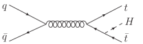
(a)

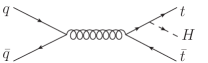
(b)

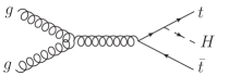
(c)

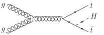
(d)

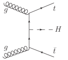
(e)

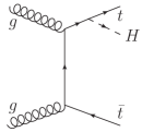
(f)

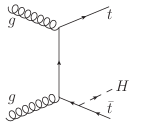
(g)

Figure 1: Tree-level Feynman diagrams contributing to $t\bar{t}H$ production at the LHC. Three more diagrams are obtained by exchanging the gluon lines in the $t$-channel diagrams.

2.1 Factorized expression for the scattering cross section

In this subsection we focus on the $gg$-initiated contributions to $t\bar{t}H$ production, since these dominate over the the quark-antiquark annihilation contributions. As we shall show below, assuming the narrow width approximation for the top and antitop quarks, the unpolarized differential cross section for $gg\to t(\to b{\ell}^{+}\nu_{\ell})\,\bar{t}(\to\bar{b}{\ell}^{-}{\bar{\nu}}_{\ell})\,H$ may be written in the following “factorized” form,

$$d\sigma=\sum_{\begin{subarray}{c}b{\ell}^{+}\nu_{l}\\ \tiny{\mathrm{spins}}\end{subarray}}\,\sum_{\begin{subarray}{c}\bar{b}{\ell}^{-}{\bar{\nu}}_{\ell}\\ \mathrm{\tiny{spins}}\end{subarray}}\left(\frac{2}{\Gamma_{t}}\right)^{2}\,d\sigma(gg\to t(n_{t})\bar{t}(n_{\bar{t}})H)\,d\Gamma(t\to b{\ell}^{+}\nu_{\ell})\,d\Gamma(\bar{t}\to\bar{b}{\ell}^{-}{\bar{\nu}}_{\ell}),$$ (2)

where $d\sigma(gg\to t(n_{t})\bar{t}(n_{\bar{t}})H)$ is the differential cross section for the production of a top and antitop quark, with spin vectors $n_{t}$ and $n_{\bar{t}}$, respectively, along with a Higgs boson. Also, $d\Gamma(t\to b{\ell}^{+}\nu_{\ell})$ and $d\Gamma(\bar{t}\to\bar{b}{\ell}^{-}{\bar{\nu}}_{\ell})$ are the partial differential decay widths for an unpolarized top and anti-top quark. The four-vectors $n_{t}$ and $n_{\bar{t}}$ are not arbitrary, but are given by particular combinations of the momenta of the $t,\bar{t},\ell^{+}$ and $\ell^{-}$ Arens ,

$$n_{t} = -\frac{p_{t}}{m_{t}}+\frac{m_{t}}{(p_{t}\cdot p_{{\ell}^{+}})}p_{{\ell}^{+}}$$ (3)

$$n_{\bar{t}} = \,\frac{p_{\bar{t}}}{m_{t}}-\frac{m_{t}}{(p_{\bar{t}}\cdot p_{{\ell}^{-}})}p_{{\ell}^{-}}.$$ (4)

Expressions similar to eq. (2) have been derived previously for the production of short-lived particles in $e^{-}e^{+}$ colliders kawasaki and for $t\bar{t}$ production both in $e^{-}e^{+}$ colliders Arens and $pp$ colliders ale1 ; ale2 ; ale3 ; ale4 .

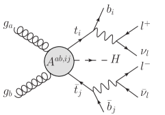
Figure 2: Schematic representation of the process $g_{a}g_{b}\to t(\to b_{i}{\ell}^{+}\nu_{\ell})\bar{t}(\to\bar{b}_{j}{\ell}^{-}{\bar{\nu}}_{\ell})H$. The indices $i,j$ denote the colours of the quarks, while $a,b$ are gluon indices.

To derive the above expressions, we begin by considering the schematic representation for the process $g_{a}g_{b}\to t(\to b_{i}{\ell}^{+}\nu_{\ell})\,\bar{t}(\to\bar{b}_{j}{\ell}^{-}{\bar{\nu}}_{\ell})\,H$ that is sketched in figure 2. Here $a$ and $b$ denote the initial-state gluons and $i$ and $j$ refer to the colours of the top and antitop quarks. The amplitude for this process may be written in the following compact form

$$\mathcal{M}^{ab,ij}=\bar{\psi}_{t}\,\mathcal{A}^{ab,ij}\,\psi_{\bar{t}}\,,$$ (5)

where the spinors $\bar{\psi}_{t}$ and $\psi_{\bar{t}}$ contain all of the information regarding the decay of the virtual top and anti-top, respectively, and where the quantity $A^{ab,ij}$ is given by

$$\mathcal{A}^{ab,ij}\equiv A^{ab,ij}_{\mu\nu}(\epsilon_{\lambda_{a}})^{\mu}(\epsilon_{\lambda_{b}})^{\nu}=\sum_{k=1}^{8}\mathcal{A}^{ab,ij}_{k}=\kappa_{t}\sum_{k=1}^{8}\mathcal{S}^{ab,ij}_{k}+i\tilde{\kappa}_{t}\sum_{k=1}^{8}\mathcal{P}^{ab,ij}_{k}.$$ (6)

The sum over $k$ in the above expression corresponds to the eight gluon-initiated diagrams indicated in figure 1; also, $\epsilon_{\lambda_{a}}$ and $\epsilon_{\lambda_{b}}$ are the polarization vectors corresponding to $g_{a}$ and $g_{b}$, respectively. In the last equality in eq. (6) we have explicitly separated the amplitude into two sums, with one sum corresponding to the scalar contributions and the other to the pseudoscalar ones. Taking all of the final-state particles to be massless, we can use the spinor techniques developed in ref. Kleiss to write $\bar{\psi}_{t}$ and $\psi_{\bar{t}}$ as follows

$$\bar{\psi}_{t}=-g^{2}\,\mathbb{P}_{t}(t)\,\mathbb{P}_{W}(t-b)\,\langle b-|\nu_{\ell}+\rangle\langle{\ell}^{+}\!+|(t\not{}\hskip 4.0pt+m_{t})$$ (7)

$$\psi_{\bar{t}}=g^{2}\,\mathbb{P}_{t}(\bar{t})\,\mathbb{P}_{W}(\bar{t}-\bar{b})\,\langle{\bar{\nu}}_{\ell}+|\bar{b}-\rangle(\bar{t}\not{}\hskip 4.0pt-m_{t})|{\ell}^{-}+\rangle,\\$$ (8)

where $|i+(-)\rangle\equiv(1/2)(1\pm\gamma^{5})\,\psi_{i}$ represents a right-handed (left-handed) chiral spinor for final-state particle $i$ and $\langle i+(-)|$ represents the corresponding adjoint spinor. Also, $\mathbb{P}_{t}(q)=(q^{2}-m^{2}_{t}+im_{t}\Gamma_{t})^{-1}$ and $\mathbb{P}_{W}(q)=(q^{2}-m^{2}_{W}+im_{W}\Gamma_{W})^{-1}$, and we have denoted the momenta of the various particles by the symbols that refer to the names of those particles Mangano .

Using the expressions defined above for $\bar{\psi}_{t}$ and $\psi_{\bar{t}}$, we can write the amplitude $\mathcal{M}^{ab,ij}$ in a form that is (in a sense) factorized. As a first step, we insert eqs. (7) and (8) into eq. (5), yielding

$$\mathcal{M}^{ab,ij}=\!-g^{4}\,\mathbb{P}_{t}(t)\,\mathbb{P}_{t}(\bar{t})\,\mathbb{P}_{W}(t-b)\,\mathbb{P}_{W}(\bar{t}-\bar{b})\,\langle b-|\nu_{\ell}+\rangle\langle{\bar{\nu}}_{\ell}+|\bar{b}-\rangle\sqrt{2(t\cdot{\ell}^{+})}\sqrt{2(\bar{t}\cdot{\ell}^{-})}\,[\bar{\phi}_{t}\mathcal{A}^{ab,ij}\phi_{\bar{t}}],$$ (9)

where the spinors $\phi_{t}$ and $\phi_{\bar{t}}$ are defined as

$$\phi_{t}=\frac{(t\not{}\hskip 4.0pt+m_{t})}{\sqrt{2(t\cdot{\ell}^{+})}}|{\ell}^{+}+\rangle$$ (10)

$$\phi_{\bar{t}}=\frac{(\bar{t}\not{}\hskip 4.0pt-m_{t})}{\sqrt{2(\bar{t}\cdot{\ell}^{-})}}|{\ell}^{-}+\rangle\,.$$ (11)

Note that in writing down the above expressions we have adopted the narrow-width approximation for the top and antitop quarks. Working out the projection operators $\phi_{t}\,\bar{\phi}_{t}$ and $\phi_{\bar{t}}\,\bar{\phi}_{\bar{t}}$, we have

$$\phi_{t}\,\bar{\phi}_{t}=\frac{1}{2}(1+n\not\hskip 4.0pt{}_{\!t}\gamma^{5})(t\not{}\hskip 4.0pt+m_{t})$$ (12)

and

$$\phi_{\bar{t}}\,\bar{\phi}_{\bar{t}}=\frac{1}{2}(1+n\not\hskip 4.0pt{}_{\!\bar{t}}\gamma^{5})(\bar{t}\not{}\hskip 4.0pt-m_{t}),$$ (13)

with $n_{t}$ and $n_{\bar{t}}$ being the four-vectors defined in eqs. (3) and (4). Thus, $\phi_{t}$ and $\phi_{\bar{t}}$ may be regarded as describing a top quark with spin vector $n_{t}$ and an antitop quark with spin vector $n_{\bar{t}}$, respectively.

As a final step toward factorizing the amplitude $\mathcal{M}^{ab,ij}$, we note that the amplitude for a top quark with spin vector $n_{t}$ to decay into $b{\ell}^{+}\nu_{\ell}$ is given by

$$\mathcal{M}(t(n_{t})\to b{\ell}^{+}\nu_{\ell})=ig^{2}\mathbb{P}_{W}(t-b)\langle b-|\nu_{\ell}+\rangle\sqrt{2(t\cdot{\ell}^{+})}\,,$$ (14)

and likewise,

$$\mathcal{M}(\bar{t}(n_{\bar{t}})\to\bar{b}{\ell}^{-}\bar{\nu}_{\ell})=ig^{2}\mathbb{P}_{W}(\bar{t}-\bar{b})\langle\bar{\nu}_{\ell}+|\bar{b}-\rangle\sqrt{2(\bar{t}\cdot{\ell}^{-})}.$$ (15)

Furthermore, the term inside the square brackets in eq. (9) is the amplitude for producing a top quark with spin vector $n_{t}$, along with an anti-top with spin vector $n_{\bar{t}}$ and a Higgs boson,

$$\mathcal{M}(g_{a}g_{b}\to t^{i}(n_{t})\bar{t}^{j}(n_{\bar{t}})H)=\bar{\phi}_{t}\mathcal{A}^{ab,ij}\phi_{\bar{t}}.$$ (16)

Combining eqs. (14)-(16), we can write eq. (9) in a form that appears to be factorized,

$$\mathcal{M}^{ab,ij}=\mathbb{P}_{t}(t)\mathbb{P}_{t}(\bar{t})\,\mathcal{M}(t(n_{t})\to b{\ell}^{+}\nu_{\ell})\,\mathcal{M}(\bar{t}(n_{\bar{t}})\to\bar{b}{\ell}^{-}\bar{\nu}_{\ell})\,\mathcal{M}(g_{a}g_{b}\to t^{i}(n_{t})\bar{t}^{j}(n_{\bar{t}})H)\,.$$ (17)

It is important to note that, even though the above expression has the appearance of being factorized into production and decay parts, this apparent factorization is a bit misleading. In particular, the amplitude for $t\bar{t}H$ production contains the top and antitop quark spin four-vectors $n_{t}$ and $n_{\bar{t}}$, which depend on final-state kinematical quantities (see eqs. (3) and (4)). With this qualification in mind, we may now use the amplitude in eq. (17) to determine the corresponding scattering cross section. After some manipulation of the phase space variables to take advantage of the presence of the propagator terms, $\mathbb{P}_{t}(t)$ and $\mathbb{P}_{t}(\bar{t})$, we arrive at the expression in eq. (2). This expression also has the appearance of being factorized, but qualifying remarks, similar to those above, apply.

2.2 Origin of triple product terms

The expression derived above for the scattering cross section (see eq. (2), as well as eq. (17)) provides significant insight into how one might analyze $pp\to t\,\left(\rightarrow b{\ell}^{+}\nu_{\ell}\right)\bar{t}\,\left(\rightarrow\bar{b}{\ell}^{-}{\bar{\nu}}_{\ell}\right)\,H$ in order to determine the nature of the top-Higgs coupling. In particular, let us focus on the production amplitude, $\mathcal{M}(g_{a}g_{b}\to t^{i}(n_{t})\bar{t}^{j}(n_{\bar{t}})H))$, which forms part of the overall amplitude in eq. (17). The absolute value squared of the production amplitude is used to determine $d\sigma(gg\to t(n_{t})\bar{t}(n_{\bar{t}})H)$, which in turn forms part of the expression for the “factorized” cross section in eq. (2). Summing over colour and gluon indices we have

$$\sum_{\begin{subarray}{c}a,b\\ i,j\end{subarray}}|\mathcal{M}(g_{a}g_{b}\to t^{i}(n_{t})\bar{t}^{j}(n_{\bar{t}})H)|^{2}=\sum_{\begin{subarray}{c}a,b\\ i,j\end{subarray}}\left|\sum^{8}_{k=1}C^{ab,ij}_{k}\,\bar{\phi}_{t}(\kappa_{t}\mathcal{S}_{k}+i\tilde{\kappa}_{t}\mathcal{P}_{k})\phi_{\bar{t}}\right|^{2},$$ (18)

where we have separated the colour structure of each diagram by defining $\mathcal{S}^{\,ab,ij}_{k}=C^{ab,ij}_{k}\mathcal{S}_{k}$ and $\mathcal{P}^{\,ab,ij}_{k}=C^{ab,ij}_{k}\mathcal{P}_{k}$ (see eqs. (6) and (16)). Also, the factors $g^{2}_{s}m_{t}/v$ and $-ig^{2}_{s}m_{t}/v$ arising from the vertices of the $t$- and $s$-channel diagrams, respectively, have been included in the definition of $C^{ab,ij}_{k}$ for convenience. The terms linear in $\kappa_{t}$ and $\tilde{\kappa}_{t}$ can be written as

$$\mathcal{O}(\kappa_{t}\tilde{\kappa}_{t})\to\frac{1}{2}\kappa_{t}\tilde{\kappa}_{t}\sum_{k,r}\mathbb{C}_{kr}\mathrm{Im}\left\{\mathrm{Tr}\left[(1+n\not\hskip 4.0pt{}_{t}\gamma^{5})(t\not{}\hskip 4.0pt+m_{t})\mathcal{S}_{k}(1+n\not\hskip 4.0pt{}_{\bar{t}}\gamma^{5})(\bar{t}\not{}\hskip 4.0pt-m_{t})\tilde{\mathcal{P}}_{r}\right]\right\},$$ (19)

where the factor $\mathbb{C}_{kr}=\sum_{ab,ij}C^{ab,ij}_{k}C^{ab,ij*}_{r}$ is real and where $\tilde{\mathcal{P}}_{r}=\gamma^{0}\mathcal{P}^{\dagger}_{r}\gamma^{0}$. The only terms that yield non-zero contributions in the above sum are those with an odd number of $\gamma^{5}$ matrices; these lead to triple-product (TP) correlations of the form $\epsilon_{\alpha\beta\gamma\delta}\,p^{\alpha}_{a}p^{\beta}_{b}p^{\gamma}_{c}p^{\delta}_{d}$, where $p_{a}$-$p_{d}$ represent various four momenta associated with the process. In contrast, it can be seen from eq. (18) that the terms proportional to $\kappa_{t}^{2}$ and $\tilde{\kappa}^{2}_{t}$ descend from traces containing an even number of $\gamma^{5}$ matrices and can be written in terms of scalar products of the available momenta.

With the above considerations in mind, it is useful to write a general expression for the differential cross section $d\sigma(gg\to t(n_{t})\bar{t}(n_{\bar{t}})H)$ in terms of the momenta $q=(q_{1}-q_{2})/2$, $Q=(q_{1}+q_{2})/2$, $t$, $\bar{t}$, $n_{t}$ and $n_{\bar{t}}$, where $q_{1,2}$ denote the momenta of the initial-state gluons. Note that with this choice, $q\cdot Q=0$ and $Q^{2}=-q^{2}=M^{2}_{t\bar{t}H}/4$, where $M_{t\bar{t}H}$ is the invariant mass of the $t\bar{t}H$ system. Fifteen TPs can be constructed from these six four-vectors, so that

$$d\sigma(gg\to t(n_{t})\bar{t}(n_{\bar{t}})H)=\kappa_{t}^{2}\,f_{1}(p_{i}\cdot p_{j})+\tilde{\kappa}^{2}_{t}\,f_{2}(p_{i}\cdot p_{j})+\kappa_{t}\tilde{\kappa}_{t}\,\sum^{15}_{l=1}g_{l}(p_{i}\cdot p_{j})\,\epsilon_{l},$$ (20)

where $\epsilon_{l}=\epsilon_{\alpha\beta\gamma\delta}\,p^{\alpha}_{a}p^{\beta}_{b}p^{\gamma}_{c}p^{\delta}_{d}$ denotes the $l$th TP (we adopt the convention $\epsilon_{0123}=+1$) and where $p_{i}$ and $p_{j}$ refer to any of the six momenta. The functions $f_{1,2}$ and $g_{k}$ depend only on the possible scalar products and are therefore even under a parity transformation ($\mathrm{P}$). However, the terms linear in $\kappa_{t}\tilde{\kappa}_{t}$ are $\mathrm{P}$-odd due to the presence of the $\mathrm{P}$-odd TPs. Hence, only the functions $f_{1,2}$ will contribute to the total cross section, whereas the TP terms will be sensitive to the sign of the anomalous coupling $\tilde{\kappa}_{t}$. Of the fifteen TPs mentioned above, we will focus on those that contain both of the spin vectors $n_{t}$ and $n_{\bar{t}}$, but do not include $q$. The decision not to consider $q$-dependent TPs is motivated by the fact that $q$ cannot be expressed in terms of the momenta of final state particles (as $Q$ can, by virtue of energy-momentum conservation). The decision to focus on TPs that contain both $n_{t}$ and $n_{\bar{t}}$ is rooted in the fact that the spins of pair-produced top and antitop quarks are highly correlated at hadron colliders (even though the quarks themselves are unpolarized). Observables that combine the decay products of the $t$ and $\bar{t}$ will be sensitive to this spin correlation Bernreuther . A similar behaviour is expected in $t\bar{t}H$ production, where it can be shown that single-spin asymmetries vanish Ellis ; Biswas . Hence, in order to construct observables sensitive to the structure of the $tH$ coupling, we will restrict our attention to those TPs that include information on the decay products of both the top and anti-top quarks. Only five of the fifteen TPs in eq. (20) do not involve the four vector $q$ and, among these, only three include both $n_{t}$ and $n_{\bar{t}}\,$. Thus, we will restrict our attention to the following TPs

$$\epsilon_{1}\equiv\epsilon(t,\bar{t},n_{t},n_{\bar{t}}),\,\,\vspace*{1mm}$$ (21)

$$\epsilon_{2}\equiv\epsilon(Q,\bar{t},n_{t},n_{\bar{t}}),\vspace*{1mm}$$ (22)

$$\epsilon_{3}\equiv\epsilon(Q,t,n_{t},n_{\bar{t}}).\vspace*{1mm}$$ (23)

Before turning to a consideration of various CP-odd observables, we remark that even though all of the above discussion took place within the context of $gg$-initiated production, similar conclusions are obtained for $q\bar{q}$-initiated production. In particular, the definitions of the spin vectors in eqs. (3)-(4) and the general form of $d\sigma$ introduced in eq. (20) are valid in both cases.

3 $\mathrm{\mathbf{CP}}$-odd observables

In this section we present three types of observables based on the TPs discussed in section 2, namely, asymmetries, angular distributions and mean values. These observables are sensitive not only to the magnitude of the pseudoscalar coupling $\tilde{\kappa}_{t}$, but also to its sign. In order to test the various observables, we have used $\mathtt{MadGraph5\_aMC@NLO}$ Madgraph to simulate the process $pp\to t\,\left(\rightarrow b{\ell}^{+}\nu_{\ell}\right)\bar{t}\,\left(\rightarrow\bar{b}{\ell}^{-}{\bar{\nu}}_{\ell}\right)\,H$ at parton level for different values of the couplings $\kappa_{t}$ and $\tilde{\kappa}_{t}$. In all cases we have generated $10^{5}$ events and have assumed a center-of-mass energy of $14\,\mathrm{TeV}$. We have also imposed the following set of cuts: $p_{T}$ of leptons $>10\,\mathrm{GeV}$, $|\eta|$ of leptons $<2.5$, $|\eta|$ of $b$ jets $<2.5$ and $\Delta R_{\ell\ell}>0.4$. Note that we have used this somewhat large number of events ($10^{5}$) in order to determine clearly the extent to which the proposed observables are sensitive to the anomalous coupling. Section 6 contains an analysis of the experimental feasibility of the more promising observables.

Before continuing on to our analysis, let us make a few comments regarding the values that we choose for $\kappa_{t}$ and $\tilde{\kappa}_{t}$. First of all, we note that if the pseudoscalar coupling $\tilde{\kappa}_{t}$ is the only source of physics beyond the SM, then indirect contraints (based on the signal strength of $gg\to H\to\gamma\gamma$) disfavour $\kappa_{t}<0$ but do not resolve the degeneracy in the sign of $\tilde{\kappa}_{t}$ Guadagnoli . On the other hand, if one assumes that the tensor structure of the Higgs interactions are the same as those of the SM and if one parameterizes these interactions via one universal Higgs coupling to vector bosons, $\kappa_{V}$, and one universal Higgs coupling to fermions, $\kappa_{f}$, then the measured signal strengths provided by the ATLAS and CMS collaborations are compatible with the values predicted by the SM, (namely, $\kappa_{f}=1$ and $\kappa_{V}=1$). With these facts in mind, we will, for the most part, set the value of the scalar coupling to its SM value ($\kappa_{t}=1$) and will allow the pseudoscalar coupling to take on various values (including both possible signs). In particular, we analyze the cases $\tilde{\kappa}_{t}=0,\pm 0.25,\pm 0.5,\pm 0.75,\pm 1$. We shall often focus on the scenarios with $\kappa_{t}=1$ and $\tilde{\kappa}_{t}=\pm 1$, which we shall refer to as the “$\mathrm{CP}$-mixed” scenarios. In addition, we also provide some analysis regarding the pure $\mathrm{CP}$-odd case ($\kappa_{t}=0,\tilde{\kappa}_{t}=1$).

3.1 Asymmetry

The first type of $\mathrm{CP}$-odd observable that we will consider is an asymmetry that compares the number of events for which a given TP is positive to that for which it is negative. Normalizing to the total number of events, we define

$$\mathcal{A}(\epsilon)=\frac{N(\epsilon>0)-N(\epsilon<0)}{N(\epsilon>0)+N(\epsilon<0)}.$$ (24)

By construction, $\mathcal{A}\in[-1,+1]$. Based on the general expression given in eq. (20), we expect the following functional form for the asymmetry,

$$\mathcal{A}(\epsilon)=\frac{A\kappa_{t}\tilde{\kappa}_{t}}{B\kappa^{2}_{t}+C\tilde{\kappa}^{2}_{t}},$$ (25)

which for $\kappa_{t}=1$ can be parameterized as

$$\mathcal{A}(\epsilon)=\frac{a\tilde{\kappa}_{t}}{1+b\tilde{\kappa}^{2}_{t}},$$ (26)

where the parameter $a\equiv A/B$ determines the sensitivity to the pseudoscalar coupling, whereas $b\equiv C/B$ quantifies the deviation from linear behaviour.

table 1 shows numerical results for the asymmetries associated with three different TPs, $\epsilon_{1}$, $\epsilon_{2}$ and $\epsilon_{3}$, taking $\kappa_{t}=1$ and $\tilde{\kappa}_{t}=0,\pm 1$. The asymmetry $\mathcal{A}$ is shown in each case, along with $\mathcal{A}/\sigma_{\mathcal{A}}$, where $\sigma_{\mathcal{A}}$ is the corresponding statistical uncertainty. As is evident from the table, the asymmetries in question provide a clear separation between the SM and the $\mathrm{CP}$-mixed cases, with typical deviations being of order $10\sigma$. Furthermore, the asymmetries for the SM case are each statistically consistent with zero, as one would expect. The three asymmetries also allow one to determine the sign of $\tilde{\kappa}_{t}$, with the $\tilde{\kappa}_{t}=\pm 1$ cases effectively separated by more than $20\sigma$. The sensitivity of the asymmetry is quite similar for the three TPs, as can be seen by including other values of $\tilde{\kappa}_{t}$ and using the expression in eq. (26) as a fitting function (see figure 3). Performing such a fit, we obtain $(a=-0.057\pm 0.006,b=0.5\pm 0.2),(a=-0.056\pm 0.006,b=0.5\pm 0.2)$ and $(a=0.058\pm 0.006,b=0.6\pm 0.2)$ for $\epsilon_{1}$, $\epsilon_{2}$ and $\epsilon_{3}$, respectively.

Table 1: Asymmetries for three different scenarios, obtained by using $10^{5}$ simulated events, for the TPs $\epsilon_{1}=\epsilon(t,\bar{t},n_{t},n_{\bar{t}}),\epsilon_{2}=\epsilon(Q,\bar{t},n_{t},n_{\bar{t}})$ and $\epsilon_{3}=\epsilon(Q,t,n_{t},n_{\bar{t}})$. The three scenarios correspond to the SM ($\kappa_{t}=1$ and $\tilde{\kappa}_{t}=0$) and the two “$\mathrm{CP}$-mixed” cases (defined by $\kappa_{t}=1$ and $\tilde{\kappa}_{t}=\pm 1$).

$\kappa_{t}$	$\tilde{\kappa}_{t}$	$\mathcal{A}(\epsilon_{1})$	$\mathcal{A}(\epsilon_{1})/\sigma_{\mathcal{A}}$	$\mathcal{A}(\epsilon_{2})$	$\mathcal{A}(\epsilon_{2})/\sigma_{\mathcal{A}}$	$\mathcal{A}(\epsilon_{3})$	$\mathcal{A}(\epsilon_{3})/\sigma_{\mathcal{A}}$
$1$	$-1$	$0.0315$	$10.0$	$0.0332$	$10.5$	$-0.0307$	$-9.7$
$1$	$0$	$-0.0021$	$-0.7$	$0.0009$	$0.3$	$-0.0011$	$-0.3$
$1$	$1$	$-0.0379$	$-12.0$	$-0.0411$	$-13.0$	$\,0.0378$	$12.0$

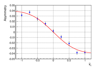
(a)

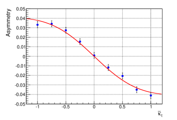
(b)

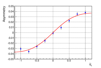
(c)

Figure 3: Asymmetries for the TPs $\epsilon_{1}=\epsilon(t,\bar{t},n_{t},n_{\bar{t}})$ (top-left), $\epsilon_{2}=\epsilon(Q,\bar{t},n_{t},n_{\bar{t}})$ (top-right) and $\epsilon_{3}=\epsilon(Q,t,n_{t},n_{\bar{t}})$ (bottom). The points represent the values for $\tilde{\kappa}_{t}=0,\pm 0.25,\pm 0.5,\pm 0.75,\pm 1$ and the red solid line is the fitting curve.

The results shown in table 1 and figure 3 all assume a $pp$ initial state, which is actually a combination of events coming from $gg$ and $q\bar{q}$ initial states. While this combination of initial states is the appropriate scenario to consider, it is interesting to consider the relative contributions to the asymmetry coming from the $gg$ and $q\bar{q}$ initial states. Figure 4 shows three curves for the “$\epsilon_{1}$” case, one for $gg$-initiated events, one for $q\bar{q}$-initiated events, and one for the usual combination of these events (the “$pp$” initial state). Interestingly, we see from figure 4 that the asymmetry for this TP is enhanced for $gg$-initiated production, while it is reduced and of opposite sign for the $q\bar{q}$-initiated events. The asymmetry for the $pp$ case is evidently dominated by the $gg$ contribution, but is somewhat smaller in magnitude due to the $q\bar{q}$ contribution.

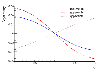
Figure 4: Asymmetry for the TP $\epsilon_{1}=\epsilon(t,\bar{t},n_{t},n_{\bar{t}})$. The dashed line (red) corresponds to $gg$-initiated production, the dot-dashed line (grey) to $q\bar{q}$-initiated production and the solid line (blue) to $pp$ production.

We have also tested various combinations of the TPs $\epsilon_{1,2,3}$ and have found that the asymmetry is enhanced for the following combination:

$$\epsilon_{4}=\epsilon_{3}-\epsilon_{2}=\epsilon(Q,t-\bar{t},n_{t},n_{\bar{t}}).$$ (27)

Note that in the $Q$ rest frame, $\epsilon_{4}=Q^{0}(\vec{t}-\vec{\bar{t}}\,)\cdot(\vec{n}_{t}\times\vec{n}_{\bar{t}})$ and the sign of this TP is determined by the quantity $(\vec{t}-\vec{\bar{t}}\,)\cdot(\vec{n}_{t}\times\vec{n}_{\bar{t}})$. The values obtained for the asymmetry associated with this TP are shown in table 2. By comparing the results in tables 1 and 2, we see that the capability of this asymmetry to distinguish between the two $\mathrm{CP}$-mixed scenarios is increased by at least $2.8\sigma$.

Table 2: Asymmetry for the TP $\epsilon_{4}$ for the SM case and the two $\mathrm{CP}$-mixed scenarios. The values are obtained using sets of $10^{5}$ simulated events.

$\kappa_{t}$	$\tilde{\kappa}_{t}$	$\mathcal{A}(\epsilon_{4})$	$\mathcal{A}(\epsilon_{4})/\sigma_{\mathcal{A}}$
$1$	$-1$	$-0.0371$	$-11.7$
$1$	$0$	$0.0004$	$0.1$
$1$	$1$	$0.0461$	$14.6$

Finally, it is worth noting that the asymmetries described in this subsection are not useful for discriminating between the SM hypothesis ($\kappa_{t}=1,\tilde{\kappa}_{t}=0$) and the pure pseudoscalar hypothesis ($\kappa_{t}=0,\tilde{\kappa}_{t}=1$). Since the numerators of the asymmetries are linear in both $\kappa_{t}$ and $\tilde{\kappa}_{t}$, they are expected to vanish in these cases. However, we will show in the next subsection that there exist angular distributions derived from the TPs that are actually suitable for distinguishing between these two hyphotheses.

3.2 Angular Distributions

Given a certain TP, it is possible to define associated angular distributions that are sensitive to the pseudoscalar coupling $\tilde{\kappa}_{t}$. In order to clarify this, let us first consider the TP $\epsilon(t,\bar{t},n_{t},n_{\bar{t}})$. This TP can be written as $\epsilon(t+\bar{t},\bar{t},n_{t},n_{\bar{t}})$, so that in the reference frame defined by $\vec{t}+\vec{\bar{t}}=0$ and $\vec{\bar{t}}\parallel\hat{z}$ we have

$$\epsilon(t+\bar{t},\bar{t},n_{t},n_{\bar{t}})=M_{t\bar{t}}\,|\vec{\bar{t}}|\,(\vec{n}_{t}\times\vec{n}_{\bar{t}})_{z}=M_{t\bar{t}}\,|\vec{\bar{t}}||\vec{n}_{t}||\vec{n}_{\bar{t}}|\sin\theta_{n_{t}}\sin\theta_{n_{\bar{t}}}\sin\Delta\phi(n_{t},n_{\bar{t}}),$$ (28)

where $M_{t\bar{t}}$ is the invariant mass of the $t\bar{t}$ pair, the angles $\theta_{n_{t}}$ and $\theta_{n_{\bar{t}}}$ denote the polar angles of $\vec{n}_{t}$ and $\vec{n}_{\bar{t}}$, respectively, and $\Delta\phi(n_{t},n_{\bar{t}})$ is the angular difference between the projections of $\vec{n}_{t}$ and $\vec{n}_{\bar{t}}$ onto the plane perpendicular to $\vec{\bar{t}}$. If we define the angle $\Delta\phi(n_{t},n_{\bar{t}})$ to be within the range $[-\pi,\pi]$, we see from eq. (28) that its sign will determine the sign of the TP. Thus, the distribution of the number of events with respect to the angle $\Delta\phi(n_{t},n_{\bar{t}})$ is related to the asymmetry of the TP,

$$\mathcal{A}(\epsilon)=1-2\frac{N(\epsilon<0)}{N_{T}}\,\,\mbox{ and }\,\,\frac{N(\epsilon<0)}{N_{T}}=\int^{0}_{-\pi}\frac{1}{N_{T}}\frac{dN}{d\Delta\phi(n_{t},n_{\bar{t}})}\,d\Delta\phi(n_{t},n_{\bar{t}}),$$ (29)

where $N_{T}$ is the total number of events. Moreover, for a certain TP one can derive different angular distributions by considering different reference frames, although all of these will satisfy eq. (29) (note that $\mathcal{A}(\epsilon)$ is Lorentz invariant). Recalling the various TPs considered in section 2, we examine the following angular distributions.

1. $\epsilon_{1}=\epsilon(t,\bar{t},n_{t},n_{\bar{t}})$. To probe $\epsilon_{1}$, we construct the distribution $d\sigma/d\Delta\phi_{1}(n_{t},n_{\bar{t}})$ in the rest frame of $t\bar{t}$, taking $\vec{\bar{t}}$ to define the $z$-axis. The angle $\Delta\phi_{1}(n_{t},n_{\bar{t}})$ is the angular difference between the projection of the spin vectors onto the plane perpendicular to $\vec{\bar{t}}$.

2. $\epsilon_{2}=\epsilon(Q,\bar{t},n_{t},n_{\bar{t}})$. In this case, we define the distribution $d\sigma/d\Delta\phi_{2}(n_{t},n_{\bar{t}})$ in the rest frame of $Q$, taking $\vec{\bar{t}}$ to define the $z$-axis. The angle $\Delta\phi_{2}(n_{t},n_{\bar{t}})$ is the angular difference between the projection of the spin vectors onto the plane perpendicular to $\vec{\bar{t}}$.

3. $\epsilon_{3}=\epsilon(Q,t,n_{t},n_{\bar{t}})$. The distribution $d\sigma/d\Delta\phi_{3}(n_{t},n_{\bar{t}})$ is also defined in the rest frame of $Q$, but this time taking $\vec{t}$ to be along the $z$-axis. The angle $\Delta\phi_{3}(n_{t},n_{\bar{t}})$ is the angular difference between the projection of the spin vectors onto the plane perpendicular to $\vec{t}$.

Figure 5 shows the normalized distributions obtained for the first case listed above. Four scenarios are considered, corresponding to the SM ($\kappa_{t}=1$ and $\tilde{\kappa}_{t}=0$), two cases in which the Higgs boson has mixed $\mathrm{CP}$ couplings ($\kappa_{t}=1$ and $\tilde{\kappa}_{t}=\pm 1$) and a case in which the Higgs boson is purely $\mathrm{CP}$-odd ($\kappa_{t}=0,\tilde{\kappa}_{t}=1$). Figure 6 shows the analogous distributions for $\epsilon_{2}$. The distributions corresponding to $\epsilon_{3}$ are similar to those of $\epsilon_{2}$, except that the “shifts” are in the opposite directions for the two $\mathrm{CP}$-mixed cases. Given the similarities of the plots we do not include them here.

As can be seen from figures 5 and 6, the peaks of the distributions are shifted to the left or the right of the origin in the $\mathrm{CP}$-mixed cases ($\kappa_{t}=1$ and $\tilde{\kappa}_{t}=\pm 1$). The magnitude of the shift appears to be approximately the same in both cases, but is in the opposite direction for $\kappa_{t}=\tilde{\kappa}_{t}=1$ compared to $\kappa_{t}=-\tilde{\kappa}_{t}=1$, thus allowing one to distinguish the sign of the pseudoscalar coupling. The observed dependence on the sign of $\tilde{\kappa}_{t}$ in these cases is consistent with the fact that the numerator of $\mathcal{A}(\epsilon)$ is linear in $\tilde{\kappa}_{t}$ (see eq. (26)) and that the quantity $N(\epsilon<0)/N_{T}$ is related to the angular distribution according to eq. (29). The angular distributions for the SM case ($\kappa_{t}=1$ and $\tilde{\kappa}_{t}=0$) and the pure pseudoscalar case ($\kappa_{t}=0$ and $\tilde{\kappa}_{t}=1$) are visibly different from each other and from the $\mathrm{CP}$-mixed scenarios. Comparing the SM and purely pseudoscalar cases, we note that while the angular distributions for the former case exhibit a minimum at $\Delta\phi_{1,2}(n_{t},n_{\bar{t}})=0$, those for the latter case exhibit a peak at this location. Thus, these two scenarios can be distinguished from each other via these angular distributions. This is to be contrasted with the situation for the asymmetries $\mathcal{A}(\epsilon)$, which vanish in both cases.

In order to quantify the shifts discussed above, we have fitted the simulated distributions with the following function, which was proposed in ref. Ellis ,

$$\frac{1}{\sigma}\frac{d\sigma}{d\Delta\phi_{i}(n_{t},n_{\bar{t}})}=a_{0}+a_{1}\cos(\Delta\phi_{i}(n_{t},n_{\bar{t}})+\delta),\qquad\,i=1,2,3.$$ (30)

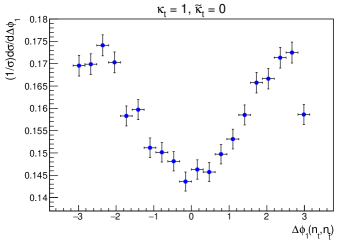
(a)

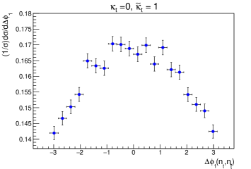
(b)

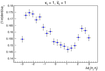
(c)

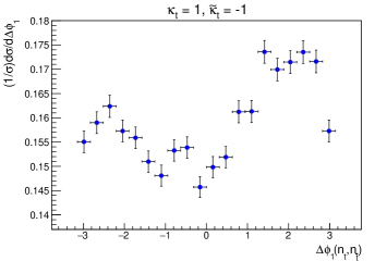
(d)

Figure 5: Angular distributions associated with the TP $\epsilon_{1}=\epsilon(t,\bar{t},n_{t},n_{\bar{t}})$ for various values of $\kappa_{t}$ and $\tilde{\kappa}_{t}$. The error bars correspond to the statistical uncertainties.

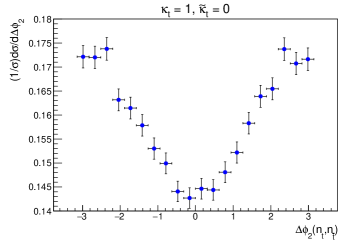
(a)

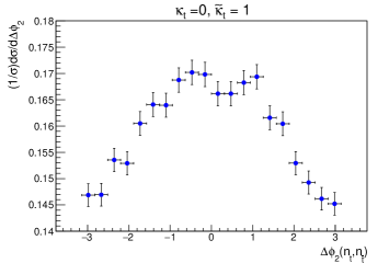
(b)

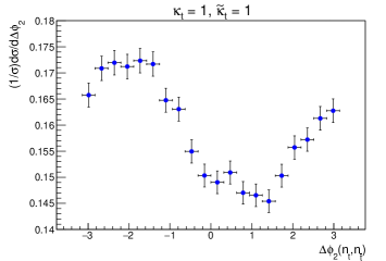
(c)

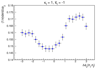
(d)

Figure 6: Angular distributions associated with the TP $\epsilon_{2}=\epsilon(Q,\bar{t},n_{t},n_{\bar{t}})$ for various values of $\kappa_{t}$ and $\tilde{\kappa}_{t}$. The error bars indicate the statistical uncertainties.

To the extent that the above expression is exact, we note that eq. (29) gives $\mathcal{A}(\epsilon_{i})=-4a_{1}\sin\delta$. With this fitting function, we obtain phase shifts $\delta$ that are approximately between $0.9$ and $1$ ($-1$ and $-0.9$) for $\kappa_{t}=-\tilde{\kappa}_{t}=1$ ($\kappa_{t}=\tilde{\kappa}_{t}=1$), both for $\epsilon_{1}$ and $\epsilon_{2}$. However, the quality of the fits in the four scenarios considered is not very good, particularly for $\epsilon_{1}$. The $\chi^{2}/\mathrm{d.o.f}$ for the fits corresponding to $\epsilon_{1}$ are in the range $1.69$-$3.86$, while for $\epsilon_{2}$ they are in the range $0.53$-$1.16$. The deviation from the functional form proposed in eq. (30) appears to be due primarily to the $\Delta R_{ll}$ cut that we have imposed. In fact, when this cut is turned off, the above ranges for the $\chi^{2}/\mathrm{d.o.f}$ become $0.75$-$1.14$ and $0.44$-$1.07$ for the $\epsilon_{1}$ and $\epsilon_{2}$ distributions, respectively. tables 3 and 4 list the results of the fits obtained when the $\Delta R_{\ell\ell}$ cut is relaxed. Figure 7 shows the corresponding plots for a couple of the scenarios. As is evident from tables 3 and 4, the parameter $\delta$ is sensitive not only to the modulus of $\tilde{\kappa}_{t}$ but also to its sign, as would be expected from eq. (29). The phase shift $\delta$ for the $\Delta\phi_{1}$ distribution appears to exhibit a slightly higher sensitivity than that obtained for the $\Delta\phi_{2}$ distribution, although the corresponding numerical values obtained for the various scenarios are compatible to within their statistical uncertainties. It is important to stress, however, that the fits for the $\Delta\phi_{2}$ distributions always yield smaller values for the $\chi^{2}/\mathrm{d.o.f}$.

In section 3.1 we defined a fourth triple product, $\epsilon_{4}=\epsilon_{3}-\epsilon_{2}$. We have constructed an angular distribution related to this TP as well. Specifically, we have analyzed the $\Delta\phi(n_{t},n_{\bar{t}})$ distribution in the $Q$ rest frame, taking $H$ to define the $z$-axis. We have studied the distributions for various values of $\kappa_{t}$ and $\tilde{\kappa}_{t}$ and have found that they are not well described by eq. (30). Instead of resembling sinusoids that are shifted to the left or right for different values of the parameters, the distributions become distorted in such a way that there is a non-zero asymmetry (see eq. (29)). Moreover, the associated asymmetry values are larger than the asymmetries for the other TPs (see tables 1 and 2).

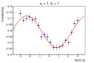
(a)

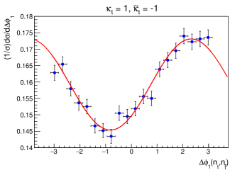
(b)

(c)

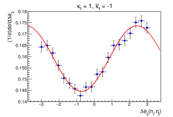
(d)

Figure 7: Angular distributions $d\sigma/(\sigma d\Delta\phi_{1}(n_{t},n_{\bar{t}}))$ (top) and $d\sigma/(\sigma d\Delta\phi_{2}(n_{t},n_{\bar{t}}))$ (bottom) associated with the TPs $\epsilon_{1}=\epsilon(t,\bar{t},n_{t},n_{\bar{t}})$ and $\epsilon_{2}=\epsilon(Q,\bar{t},n_{t},n_{\bar{t}})$, respectively, for the $\mathrm{CP}$-mixed cases $\kappa_{t}=\tilde{\kappa}_{t}=1$ (left) and $\kappa_{t}=-\tilde{\kappa}_{t}=1$ (right). The $\Delta R_{\ell\ell}$ cut was turned off when generating these results. The corresponding fit curves (see eq. (30)) are displayed in red.

Table 3: Fit results for the angular distribution $d\sigma/(\sigma d\Delta\phi_{1}(n_{t},n_{\bar{t}}))$ (related to the TP $\epsilon_{1}=\epsilon(t,\bar{t},n_{t},n_{\bar{t}})$) with the $\Delta R_{\ell\ell}$ cut turned off. Note that the sign of the parameter $a_{1}$ changes for $\kappa_{t}=0,\kappa_{t}=1$, compared to the other cases. We restrict $\delta$ to be between $\pm\pi/2$.

$\kappa_{t}$	$\tilde{\kappa}_{t}$	$a_{0}$	$a_{1}$	$\delta$
$1$	$-1$	$0.1592\pm 0.0006$	$-0.0139\pm 0.0008$	$0.81\pm 0.07$
$1$	$0$	$0.1595\pm 0.0006$	$-0.0181\pm 0.0008$	$0.002\pm 0.06\,\,$
$1$	$1$	$0.1591\pm 0.0006$	$-0.0131\pm 0.0008$	$\,-0.82\pm 0.07\quad$
$0$	$1$	$0.1591\pm 0.0006$	$\,0.0102\pm 0.0008$	$0.11\pm 0.08$

Table 4: Fit results for the angular distribution $d\sigma/(\sigma d\Delta\phi_{2}(n_{t},n_{\bar{t}}))$ (related to the TP $\epsilon_{2}=\epsilon(Q,\bar{t},n_{t},n_{\bar{t}})$), with the $\Delta R_{\ell\ell}$ cut turned off. As was the case in table 3, the sign of the parameter $a_{1}$ changes for $\kappa_{t}=0,\kappa_{t}=1$ and we restrict $\delta$ to be between $\pm\pi/2$.

$\kappa_{t}$	$\tilde{\kappa}_{t}$	$a_{0}$	$a_{1}$	$\delta$
$1$	$-1$	$0.1591\pm 0.0006$	$-0.0146\pm 0.0008$	$0.73\pm 0.06$
$1$	$0$	$0.1594\pm 0.0007$	$-0.0190\pm 0.0008$	$0.005\pm 0.06\,\,$
$1$	$1$	$0.1592\pm 0.0006$	$-0.0136\pm 0.0008$	$\,-0.77\pm 0.07\quad$
$0$	$1$	$0.1591\pm 0.0006$	$\,0.0113\pm 0.0008$	$0.09\pm 0.08$

3.3 Mean value

We turn now to consider the last type of observable that we will construct from the TPs, the mean value. As was the case for the observables considered in sections 3.1 and 3.2, the mean value is sensitive to $\tilde{\kappa}_{t}$. Given a certain TP, we define its mean value in the following manner,

$$\langle\epsilon\rangle=\frac{\int\epsilon\,[d\sigma(pp\to b\,\ell^{+}\nu_{\ell}\,\bar{b}\,\ell^{-}\bar{\nu}_{\ell}H)/d\Phi]\,d\Phi}{\int[d\sigma(pp\to b\,\ell^{+}\nu_{\ell}\,\bar{b}\,\ell^{-}\bar{\nu}_{\ell}H)/d\Phi]\,d\Phi},$$ (31)

where $\Phi$ is the Lorentz-invariant phase space corresponding to the final state $b\,\ell^{+}\nu_{\ell}\,\bar{b}\,\ell^{-}\bar{\nu}_{\ell}H$. From eq. (20) we see that only the terms linear in (both) $\kappa_{t}$ and $\tilde{\kappa}_{t}$ will contribute to the mean value. Thus, we expect this observable to be sensitive not only to the magnitude of $\kappa_{t}\tilde{\kappa}_{t}$, but also to the relative sign of the couplings.

The results obtained for the TPs $\epsilon_{1}=\epsilon(t,\bar{t},n_{t},n_{\bar{t}})$, $\epsilon_{2}=\epsilon(Q,\bar{t},n_{t},n_{\bar{t}})$ and $\epsilon_{3}=\epsilon(Q,t,n_{t},n_{\bar{t}})$ introduced in section 2 are displayed in table 5. For each TP we list the mean value divided by the corresponding statistical uncertainty. We see that the three observables are capable of distinguishing the SM case from both $\mathrm{CP}$-mixed cases. Furthermore, the two $\mathrm{CP}$-mixed cases are clearly disentangled, since the observables are sensitive to the sign of $\tilde{\kappa}_{t}$. The observables $\langle\epsilon_{2}\rangle$ and $\langle\epsilon_{3}\rangle$ appear to be slightly more sensitive than $\langle\epsilon_{1}\rangle$. Also, the mean value for the combination $\epsilon_{4}$ introduced in section 3.1 is slightly less sensitive than $\langle\epsilon_{1}\rangle$, $\langle\epsilon_{2}\rangle$ and $\langle\epsilon_{3}\rangle$, with values $-4.32$, $1.11$ and $7.23$ for the cases $(\kappa_{t}=1,\tilde{\kappa}_{t}=-1,0,1)$, respectively. As with the asymmetry, the purely $\mathrm{CP}$-even and purely $\mathrm{CP}$-odd cases cannot be distinguished by the mean value, since it is linear in both $\kappa_{t}$ and $\tilde{\kappa}_{t}$ (see eqs. (20) and (31)). Comparing the results in table 5 with the results presented in section 3.1, we can conclude that the sensitivity to the anomalous $tH$ coupling is smaller for the mean values of the TPs under consideration than for the corresponding asymmetries.

Table 5: Mean values obtained for the TPs $\epsilon_{1,2,3}$ for the SM case and two $\mathrm{CP}$-mixed cases. The values are obtained using a sample of $10^{5}$ simulated events.

$\kappa_{t}$	$\tilde{\kappa}_{t}$	$\langle\epsilon_{1}\rangle/\sigma_{\bar{\epsilon}_{1}}$	$\langle\epsilon_{2}\rangle/\sigma_{\bar{\epsilon}_{2}}$	$\langle\epsilon_{3}\rangle/\sigma_{\bar{\epsilon}_{3}}$
$1$	$-1$	$4.26$	$4.94$	$-5.81$
$1$	$0$	$-0.91$	$-0.22$	$1.25$
$1$	$1$	$-7.98$	$-8.83$	$8.75$

4 $\mathrm{CP}$-odd observables not depending on $t$ and $\bar{t}$ spin vectors

So far we have considered TPs involving the momenta $t,\bar{t}$ and $Q$ and the spin vectors $n_{t}$ and $n_{\bar{t}}$ [defined in eqs. (3)-(4)]. Furthermore, we have described the general form of the differential cross section in terms of these vectors in eq. (20). In this section we consider other possibilities for the choice of the vectors from which the $\mathrm{CP}$-odd observables can be constructed. From the definitions in eqs. (3) and (4), we see that the TPs $\epsilon_{1,2,3}$ can be written as follows,

$$\epsilon(t,\bar{t},n_{t},n_{\bar{t}})=\frac{m^{2}_{t}}{(t\cdot\ell^{+})(\bar{t}\cdot\ell^{-})}\,\epsilon(t,\bar{t},\ell^{-}\!,\ell^{+}),$$ (32)

$$\epsilon(Q,\bar{t},n_{t},n_{\bar{t}})=\frac{m^{2}_{t}}{(t\cdot\ell^{+})(\bar{t}\cdot\ell^{-})}\left(\epsilon(t,\bar{t},\ell^{-}\!,\ell^{+})+\epsilon(H,\bar{t},\ell^{-}\!,\ell^{+})+\frac{(t\cdot\ell^{+})}{m^{2}_{t}}\epsilon(H,\bar{t},t,\ell^{-}\!)\right)\,,$$ (33)

$$\epsilon(Q,t,n_{t},n_{\bar{t}})=\frac{m^{2}_{t}}{(t\cdot\ell^{+})(\bar{t}\cdot\ell^{-})}\left(-\epsilon(t,\bar{t},\ell^{-}\!,\ell^{+})+\epsilon(H,t,\ell^{-}\!,\ell^{+})+\frac{(\bar{t}\cdot\ell^{-})}{m^{2}_{t}}\epsilon(H,\bar{t},t,\ell^{+}\!)\right).\vspace*{2mm}$$ (34)

The above equations express the TPs studied in the last sections as a combination of TPs involving the momenta $t,\bar{t},H,\ell^{+}$ and $\ell^{-}$, with coefficients that are functions of phase space variables. These five momenta give rise to five TPs whose sensitivity can also be tested by means of the observables introduced in sections 3.1-3.3. We have found that TPs that do not include both the lepton and anti-lepton momenta yield negligible sensitivity to the value of $\tilde{\kappa}_{t}$. For this reason, we concentrate here on the results obtained for the remaining TPs,

$$\epsilon_{5}\equiv\epsilon(t,\bar{t},\ell^{-}\!,\ell^{+})\,,\vspace*{1mm}$$ (35)

$$\epsilon_{6}\equiv\epsilon(H,t,\ell^{-}\!,\ell^{+})\,,\vspace*{1mm}$$ (36)

$$\epsilon_{7}\equiv\epsilon(H,\bar{t},\ell^{-}\!,\ell^{+})\,.\vspace*{1mm}$$ (37)

tables 6 and 7 summarize the results for the TPs $\epsilon_{5,6,7}$. We see that $\epsilon_{5}$ gives rise to asymmetries and mean values that are clearly larger than those obtained for $\epsilon_{6}$ and $\epsilon_{7}$. This is in contrast to the TPs $\epsilon_{1,2,3}$, for which the asymmetries and mean values are comparable among the TPs (see tables 1 and 5). We also note that the asymmetry for $\epsilon_{5}$ is exactly the same as for $\epsilon_{1}$, as is expected from eq. (32), since the proportionality factor relating them is positive definite. Regarding the mean values, we see by comparing tables 5 and 7 that the TPs $\epsilon_{1,2,3}$ appear to have a higher sensitivity to the pseudoscalar coupling than do $\epsilon_{5,6,7}$.

Table 6: Asymmetries for the TPs $\epsilon_{5,6,7}$ for the SM case and the two $\mathrm{CP}$-mixed cases. The values correspond to $10^{5}$ simulated events.

$\kappa_{t}$	$\tilde{\kappa}_{t}$	$\mathcal{A}(\epsilon_{5})$	$\mathcal{A}(\epsilon_{5})/\sigma_{\mathcal{A}}$	$\mathcal{A}(\epsilon_{6})$	$\mathcal{A}(\epsilon_{6})/\sigma_{\mathcal{A}}$	$\mathcal{A}(\epsilon_{7})$	$\mathcal{A}(\epsilon_{7})/\sigma_{\mathcal{A}}$
$1$	$-1$	$0.0315$	$10.0$	$-0.0134$	$-4.2$	$0.0111$	$3.5$
$1$	$0$	$-0.0021$	$-0.7$	$-0.0011$	$-0.3$	$0.0009$	$0.3$
$1$	$1$	$-0.0379$	$-12.0$	$0.0143$	$4.5$	$-0.0137$	$\,-4.3$

Table 7: Mean values obtained for $\epsilon_{5,6,7}$ for the SM case and the two $\mathrm{CP}$-mixed cases. The values correspond to $10^{5}$ simulated events.

$\kappa_{t}$	$\tilde{\kappa}_{t}$	$\langle\epsilon_{5}\rangle/\sigma_{\bar{\epsilon}_{5}}$	$\langle\epsilon_{6}\rangle/\sigma_{\bar{\epsilon}_{6}}$	$\langle\epsilon_{7}\rangle/\sigma_{\bar{\epsilon}_{7}}$
$1$	$-1$	$3.98$	$-1.96$	$1.69$
$1$	$0$	$-0.43$	$1.25$	$0.74$
$1$	$1$	$-6.76$	$3.46$	$-3.29$

It is important to mention that in the $t\bar{t}$ rest frame the sign of the TP $\epsilon_{5}$ is defined through the angle $\Delta\phi(\ell^{-},\ell^{+})$ (see the discussion following eq. (28)), which is the angular difference between the projections of the leptons’ momenta onto the plane perpendicular to $\vec{\bar{t}}$. As in section 3.2, we can construct an associated angular distribution (see eq. (29)) that will be sensitive to the sign of the pseudoscalar coupling. The angular variable $\Delta\phi(\ell^{-},\ell^{+})$ is the same as that proposed in ref. Ellis as a useful $\mathrm{CP}$-odd observable. Moreover, it is shown in ref. Ellis that the corresponding angular distribution follows the functional form given in eq. (30). The associated shifts ($\delta$) obtained for different values of $\tilde{\kappa}_{t}$ are expected to be of the same order as those exhibited by the $\Delta\phi_{1}(n_{t},n_{\bar{t}})$ distribution since the $\Delta\phi(\ell^{-},\ell^{+})$ distribution is constrained by the asymmetry $\mathcal{A}(\epsilon_{5})$ [via eq. (29)], which in turn is equal to $\mathcal{A}(\epsilon_{1})$. Also, we note that $\mathcal{A}(\epsilon_{5})$ is slightly less sensitive than $\mathcal{A}(\epsilon_{2})$, as can be seen from table 1.

In addition to the $\epsilon_{5}$ angular distribution (defined above), one can also define angular distributions corresponding to $\epsilon_{6}$ and $\epsilon_{7}$. As was the case for the $\epsilon_{5}$ distribution, the corresponding angles will be defined in terms of the momenta of the leptons instead of in terms of the spin vectors (as was done in section 3.2). The angular distributions based on $\epsilon_{5}$-$\epsilon_{7}$ have the same overall behaviour as those derived from $\epsilon_{1}$-$\epsilon_{3}$. Using eq. (30) to fit the distributions and comparing to the results obtained for $\epsilon_{1}$-$\epsilon_{3}$, we find that the phase shifts ($\delta$) are comparable for the $\epsilon_{5}$ angular distribution, but are smaller for the $\epsilon_{6}$ and $\epsilon_{7}$ distributions.

In analogy with the combination of TPs considered in section 3, we have found a combination of the TPs $\epsilon_{5,6,7}$ for which the asymmetry is enhanced compared to those for $\epsilon_{5}$-$\epsilon_{7}$,

$$\epsilon_{8}=2\epsilon_{5}-\epsilon_{6}+\epsilon_{7}=\epsilon(t+\bar{t}+H,t-\bar{t},\ell^{+},\ell^{-}).$$ (38)

We see from eq. (38) that in the $t\bar{t}H$ rest frame $\epsilon_{8}=M_{t\bar{t}H}(\vec{t}-\vec{\bar{t}})\cdot(\vec{\ell}^{+}\!\times\vec{\ell}^{-})$, where $M_{t\bar{t}H}$ is the invariant mass of the $t\bar{t}H$ system. Hence, in the $t\bar{t}H$ rest frame the sign of $\epsilon_{8}$ is determined by the quantity $(\vec{t}-\vec{\bar{t}})\cdot(\vec{\ell}^{+}\!\times\vec{\ell}^{-})$. Comparing eqs. (27) and (38), and noting that $Q=(t+\bar{t}+H)/2$, we see that the only relevant difference between $\epsilon_{4}$ and $\epsilon_{8}$ is that in the latter the spin vectors $n_{t}$ and $n_{\bar{t}}$ have been replaced by the momenta of the leptons $\ell^{+}$ and $\ell^{-}$, respectively. The values obtained for $\mathcal{A}(\epsilon_{8})$ are shown in table 8. Compared to the TPs $\epsilon_{1}$-$\epsilon_{3}$ and $\epsilon_{5}$-$\epsilon_{7}$ (see tables 1 and 6), the asymmetry for $\epsilon_{8}$ has a comparable or slightly higher sensitivity for resolving the $\mathrm{CP}$-mixed cases. Comparing with $\mathcal{A}(\epsilon_{4})$, however, we see that using the momenta of the leptons (in $\epsilon_{8}$) instead of the spin vectors produces a decrease in the sensitivity of the asymmetry (see tables 2 and 8).

The mean values of $\epsilon_{8}$ for the scenarios under consideration are comparable with the values listed in table 7 for $\epsilon_{5}$. We have also studied the associated angular distributions. Specifically, we have analyzed the $\Delta\phi(\ell^{+},\ell^{-})$ distribution in the $t\bar{t}H$ rest frame, taking $H$ to define the $z$-axis. The distributions obtained for different values of $\kappa_{t}$ and $\tilde{\kappa}_{t}$ are not well described by eq. (30) (the situation is similar to that encountered for the angular distribution associated with $\epsilon_{4}$ – see the discussion at the end of section 3.2.). For different values of the parameters, the distributions become slightly distorted giving rise to a non-zero asymmetry (see eq. (29)).

Table 8: Asymmetry for the TP $\epsilon_{8}$ for the SM case and the two $\mathrm{CP}$-mixed scenarios. The values are obtained with $10^{5}$ simulated events.

$\kappa_{t}$	$\tilde{\kappa}_{t}$	$\mathcal{A}(\epsilon_{8})$	$\mathcal{A}(\epsilon_{8})/\sigma_{\mathcal{A}}$
$1$	$-1$	$0.0331$	$10.5$
$1$	$0$	$0.0023$	$0.7$
$1$	$1$	$-0.0403$	$\,-12.7$

5 $\mathrm{CP}$-odd observables not depending on $t$ and $\bar{t}$ momenta

The observables discussed in the preceding sections all involve the momenta of the top and/or anti-top quarks and thus require the full reconstruction of the kinematics of the individual $t$ and $\bar{t}$ systems in order to be measured. Although challenging due to the presence of the two neutrinos in the final state, this can in principle be done by applying a kinematic reconstruction algorithm (we will come back to this point in the next section). Another possibility is to define observables that do not depend on the $t$ and $\bar{t}$ momenta but instead make use of the momenta of the $b$ and $\bar{b}$ quarks to which the $t$ and $\bar{t}$ decay. In order to construct such observables we will take as our starting point the most sensitive observables studied in sections 3 and 4, namely those associated with the TPs $\epsilon_{4}$ and $\epsilon_{8}$, respectively.

Let us first consider the TP combination $\epsilon_{8}$, which is defined in eq. (38). Replacing the momenta of the $t$ and $\bar{t}$ quarks by the momenta of the $b$ and $\bar{b}$ quarks, respectively, we have a new TP,

$$\epsilon_{9}=\epsilon(b+\bar{b}+H,b-\bar{b},\ell^{+},\ell^{-}).$$ (39)

Note that the sign of $\epsilon_{9}$ is determined by the sign of the quantity $(\vec{b}-\vec{\bar{b}})\cdot(\vec{\ell}^{+}\!\times\vec{\ell}^{-})$ in the $b\bar{b}H$ rest frame. This combination of three vectors (determined in the lab frame instead of the $b\bar{b}H$ rest frame) is used in ref. Guadagnoli to define a $\mathrm{CP}$-odd observable that only depends on lab frame variables. The values of the asymmetry for $\epsilon_{9}$ are listed in table 9. Comparing tables 8 and 9 we see that the use of the $b$ and $\bar{b}$ momenta instead of the $t$ and $\bar{t}$ momenta leads to a decrease in the sensitivity of the asymmetry by $\sim 5\sigma$ for $\kappa_{t}=1,\tilde{\kappa}_{t}=\pm 1$. Nevertheless, the observable can still discriminate not only between the two $\mathrm{CP}$-mixed scenarios but also between these and the SM case.

Table 9: Asymmetry for the TP $\epsilon_{9}$ for the SM case and the two $\mathrm{CP}$-mixed cases. The values are obtained with $10^{5}$ simulated events.

$\kappa_{t}$	$\tilde{\kappa}_{t}$	$\mathcal{A}(\epsilon_{9})$	$\mathcal{A}(\epsilon_{9})/\sigma_{\mathcal{A}}$
$1$	$-1$	$0.0171$	$5.4$
$1$	$0$	$0.0010$	$0.3$
$1$	$1$	$-0.0247$	$\,-7.8$

We proceed in a similar manner with the TP $\epsilon_{4}$. Starting from eq. (27) and using the definitions of the spin vectors in eqs. (3) and (4), we have

$$\epsilon_{4}=\frac{m^{2}_{t}}{(t\cdot\ell^{+})\cdot(\bar{t}\cdot\ell^{-})}\,\epsilon(Q,t-\bar{t},\ell^{-},\ell^{+})+\frac{1}{(t\cdot\ell^{+})}\,\epsilon(Q,t,\ell^{+},\bar{t})-\frac{1}{(\bar{t}\cdot\ell^{-})}\,\epsilon(Q,\bar{t},t,\ell^{-}).$$ (40)

Since the asymmetry is not changed by the presence of an overall positive definite multiplicative factor, let us concentrate instead on the following combination of TPs,

$$\epsilon(Q,t-\bar{t},\ell^{-},\ell^{+})+\frac{(\bar{t}\cdot\ell^{-})}{m^{2}_{t}}\epsilon(Q,t,\ell^{+},\bar{t})-\frac{(t\cdot\ell^{+})}{m^{2}_{t}}\epsilon(Q,\bar{t},t,\ell^{-}).$$ (41)

Instead of replacing $t$ and $\bar{t}$ directly by $b$ and $\bar{b}$, we use the visible contributions, namely $b+\ell^{+}$ and $\bar{b}+\ell^{-}$, respectively. This results in the following definition

$$\epsilon_{10}=\epsilon(\tilde{Q},c_{b\bar{b}}\,,\ell^{-},\ell^{+})-w_{1}\,\epsilon(\tilde{Q},b,\bar{b},\ell^{+})+w_{2}\,\epsilon(\tilde{Q},b,\bar{b},\ell^{-}),$$ (42)

where $\tilde{Q}\equiv(b+\ell^{+}\!+\bar{b}+\ell^{-})/2$ stands for the visible part of $Q$, $c_{b\bar{b}}=(1-w_{1})\,b-(1-w_{2})\,\bar{b}$, and the weights $w_{1,2}$ are given by $(\bar{b}\cdot\ell^{-})/m^{2}_{t}$ and $(b\cdot\ell^{+})/m^{2}_{t}$, respectively. Also, the contribution $m^{2}_{\ell}/m^{2}_{t}$ has been neglected both in $w_{1}$ and in $w_{2}$. Note that if we set $w_{1}=w_{2}=0$, the combination $\epsilon_{10}$ reduces to $\epsilon_{9}/2$ and $\mathcal{A}(\epsilon_{10})$ becomes equal to $\mathcal{A}(\epsilon_{9})$. The results obtained for the asymmetry of $\epsilon_{10}$ are given in table 10. By comparing tables 2 and 10 we see again that the sensitivity of the asymmetry decreases when $t$ and $\bar{t}$ are not included in the TP. Nevertheless, the combination $\epsilon_{10}$ remains a useful observable for discriminating the $\mathrm{CP}$ nature of the Higgs boson, with the corresponding asymmetry having a sensitivity that is higher than that of $\epsilon_{9}$.

Comparing tables 9 and 10, we see that the effective separation between the $\mathrm{CP}$-mixed scenarios is enhanced by about $3\sigma$ for $\mathcal{A}(\epsilon_{10})$ compared to $\mathcal{A}(\epsilon_{9})$. This improvement in the asymmetry may be due to two facts. In the first place, as was pointed out in section 4 when comparing the TPs $\epsilon_{4}$ and $\epsilon_{8}$, the asymmetry appears to be higher when the spin vectors are used instead of the lepton momenta. We see from eqs. (39) and (42) that $\epsilon_{10}$, being obtained from $\epsilon_{4}$, contains the information on the spin vectors; by way of contrast, $\epsilon_{9}$ depends directly on the lepton momenta because it is derived from $\epsilon_{8}$. In the second place, in order to obtain $\epsilon_{10}$, we have replaced the top and antitop momenta by their visible parts, while in the case of $\epsilon_{9}$ the bottom and antibottom momenta have been used.

For comparison purposes, we have also used our simulated events to test the lab frame

Table 10: Asymmetry for the TP $\epsilon_{10}$ for the SM case and the two $\mathrm{CP}$-mixed cases. The values are obtained by using $10^{5}$ simulated events.

$\kappa_{t}$	$\tilde{\kappa}_{t}$	$\mathcal{A}(\epsilon_{10})$	$\mathcal{A}(\epsilon_{10})/\sigma_{\mathcal{A}}$
$1$	$-1$	$-0.0213$	$-6.7$
$1$	$0$	$0.0031$	$1.0$
$1$	$1$	$0.0300$	$9.5$

observable given in ref. Guadagnoli . We have found that this observable appears to be slightly less sensitive than $\mathcal{A}(\epsilon_{10})$, giving rise to an effective separation between the $\mathrm{CP}$-mixed scenarios that is smaller by about $1.4\sigma$.

6 Experimental Feasibility

In our numerical analyses so far we have used relatively large samples of events ($10^{5}$ events per sample) in order to clearly distinguish which observables would be most promising. The number of events expected at the High Luminosity Large Hadron Collider (HL-LHC), however, is smaller than the number of events that we have used in our simulations. In this section we reexamine the more promising observables, using sample sizes that are more attainable in the near future.

Let us first make some estimates regarding the number of signal events expected at the HL-LHC. In section 3 we introduced several mild selection cuts. Implementing these cuts, and assuming that the final state leptons could be either electrons or muons, the SM cross section for $pp\to t\,\left(\rightarrow b{\ell}^{+}\nu_{\ell}\right)\bar{t}\,\left(\rightarrow\bar{b}{\ell}^{-}{\bar{\nu}}_{\ell}\right)\,H$ at $14\,\mathrm{TeV}$ is $\sim 15.3\,\mathrm{fb}$; thus, the number of events expected within the context of the HL-LHC is $\sim 15.3\,\mathrm{fb}\times 3000\,\mathrm{fb}^{-1}=4.59\times 10^{4}$. This number is expected to be larger if $\tilde{\kappa}_{t}\neq 0$ (assuming $\kappa_{t}=1$), since the corresponding cross section is larger than the SM cross section in this case. Taking into account NLO corrections (to the production process) via a $K$ factor of approximately $1.2$ Dawson ; Beenakker ; Dittmaier , we find that the expected number of events increases to $\sim 5.5\times 10^{4}$. On the other hand, additional cuts, as well as a reduction in efficiency related to momentum reconstruction, will lead to a decrease in this number.

Given the discussion in the previous paragraph, we have generated sets of $5\times 10^{4},1\times 10^{4}$ and $5\times 10^{3}$ events and have recalculated the most sensitive observable, $\mathcal{A}(\epsilon_{4})$, for each case. The results are displayed in table 11, where it can be seen that for $5\times 10^{4}$ events (which is close to our rough estimate above for the total number of signal events for the HL-LHC), the observable is still very sensitive to $\tilde{\kappa}_{t}$. In this case, the $\mathrm{CP}$-mixed scenarios are effectively separated by $19\sigma$. As expected, the sensitivity worsens as the number of events is reduced, but even with $5\times 10^{3}$ events the effective separation between the $\mathrm{CP}$-mixed scenarios under consideration is $6.5\sigma$.

In section 5 we defined the TP combination $\epsilon_{10}$, which does not depend directly on the top or antitop momenta. Although the top and antitop momenta would not need to be reconstructed to measure $\mathcal{A}(\epsilon_{10})$, it is still useful to examine this observable for more conservative numbers of events. table 12 shows the results obtained for $5\times 10^{4}$ and $1\times 10^{4}$ events. We see in this case that even with $1\times 10^{4}$ events the observable is able to distinguish the $\mathrm{CP}$-mixed cases by $5.6\sigma$.

Table 11: Asymmetry for the TP $\epsilon_{4}$ obtained using $5\times 10^{4},1\times 10^{4}$ and $5\times 10^{3}$ events for the SM case and the two $\mathrm{CP}$-mixed cases.

$\kappa_{t}$	$\tilde{\kappa}_{t}$	$N_{\mathrm{ev}}=5\times 10^{4}$		$N_{\mathrm{ev}}=1\times 10^{4}$		$N_{\mathrm{ev}}=5\times 10^{3}$
		$\mathcal{A}(\epsilon_{4})$	$\mathcal{A}(\epsilon_{4})/\sigma_{\mathcal{A}}$	$\mathcal{A}(\epsilon_{4})$	$\mathcal{A}(\epsilon_{4})/\sigma_{\mathcal{A}}$	$\mathcal{A}(\epsilon_{4})$	$\mathcal{A}(\epsilon_{4})/\sigma_{\mathcal{A}}$
$1$	$-1$	$-0.0405$	$-9.1$	$-0.0426$	$-4.3$	$-0.0496$	$-3.5$
$1$	$0$	$0.0004$	$0.1$	$-0.0084$	$-0.8$	$-0.0004$	$-0.03$
$1$	$1$	$0.0443$	$9.9$	$0.0434$	$4.2$	$\,0.0420$	$3.0\,\,$

Table 12: Asymmetry for the TP $\epsilon_{10}$ in the SM case and the two $\mathrm{CP}$-mixed cases for $5\times 10^{4}$ and $1\times 10^{4}$ events.

$\kappa_{t}$	$\tilde{\kappa}_{t}$	$N_{\mathrm{ev}}=5\times 10^{4}$		$N_{\mathrm{ev}}=1\times 10^{4}$
		$\mathcal{A}(\epsilon_{10})$	$\mathcal{A}(\epsilon_{10})/\sigma_{\mathcal{A}}$	$\mathcal{A}(\epsilon_{10})$	$\mathcal{A}(\epsilon_{10})/\sigma_{\mathcal{A}}$
$1$	$-1$	$-0.0270$	$-6.0$	$-0.0184$	$-1.8$
$1$	$0$	$0.0022$	$0.5$	$-0.0086$	$-0.9$
$1$	$1$	$0.0313$	$7.0$	$0.0380$	$3.8\,$

We note that in order to be fully conclusive about the required luminosity, it is important to include the effects of hadronization, detector resolution, reconstruction efficiencies and so forth. In fact, the measurement of some of the proposed observables necessitates the reconstruction of the $t$ and $\bar{t}$ momenta. Such is the case, for example, for the most sensitive observable, the asymmetry $\mathcal{A}(\epsilon_{4})$.

The determination of the kinematic quantities associated with the top quark and antiquark is challenging, not only due to the presence of the two neutrinos in the final state (which escape the detector undetected), but also because the (visible) quarks and charged leptons in the final state need to be correctly associated with the corresponding parent particle (i.e., the top or antitop quark). Even in the case in which two leptons and two jets are reconstructed, there are still two possibilities for associating the $b$ jets with the appropriate parent particles. Regarding the momenta of the neutrinos, the six unknowns (corresponding to the three-momenta of the two neutrinos) can be determined by using the six kinematic equations following from the conservation of the transverse momentum and from the $W^{\pm}$ and $t$ and $\bar{t}$ invariant mass constraints. As is shown in ref. Sonnenschein , the resulting set of equations can be reduced to one univariate polynomial of degree four, leading to the possibility of obtaining up to four solutions. In addition to these various challenges, the impact of the finite detector resolution on finding the solution of the kinematic equations has to be taken into account. There are various methods of kinematic reconstruction that deal with these problems and allow for the reconstruction of the kinematical properties of the top-quark pair from the four-momenta of the final-state particles. The following describes two kinematic reconstruction methods used recently by the ATLAS and CMS collaborations.

• The first method is known as the neutrino weighting technique and is based on ref. Abbott . In this approach, the kinematic equations are used with the reconstructed jets, leptons and $\vec{E}_{T}\not{}\hskip 12.0pt$ as inputs and the masses of the $W$ bosons, the $t$ and the $\bar{t}$ are fixed. The pseudorapidities corresponding to the two neutrinos are sampled by using a simulated neutrino energy spectrum and, in order to include detector resolution effects, the reconstructed jets are smeared. Each solution obtained by scanning over the two pseudorapidities for each smearing step are weighted according to the agreement between the calculated and measured $\vec{E}_{T}\not{}\hskip 12.0pt$. For each event, the measurement of a given observable is obtained as the respective weighted mean value. Within the context of $t\bar{t}$ production this procedure has been used, for instance, to obtain spin correlation atlasconf and charge asymmetry atlascharge measurements in the dileptonic decay channel. In the former case, the reconstruction efficiency is approximately $95\%$ for simulated $t\bar{t}$ events, while in the latter case this efficiency is estimated to be $80\%$ for the experimental data set.

• The second method also uses the kinematic equations with the reconstructed objects as inputs, but in contrast to the previous method, only the top quark mass is fixed (to the value $m_{t}=172.5\,\mathrm{GeV}$); the $W$ mass is smeared according to the true $W$ mass distribution. The energies and the directions of the reconstructed jets and leptons are smeared $100$ times and events with two $b$-tagged jets are preferred compared to those with one $b$-tagged jet. For each lepton-jet pair a weight is assigned based on the expected true lepton-$b$-jet invariant mass spectrum, and the pair with the highest sum (over the smearings) of weights is chosen. For each of the $100$ smearings of this lepton-jet pair, the ambiguity in the solution of the kinematics equations is resolved by taking the solution giving the smallest invariant mass of the $t\bar{t}$ system. Finally, the kinematic quantities associated with the top quark and antiquark are obtained as a weighted average according to the true $m_{b\ell}$ distribution. This technique has been used in ref. CMS2 to measure the differential cross-section for $t\bar{t}$ production in the dileptonic decay channel. The reconstruction efficiency reported is $\sim 94\%$, which is a $\sim 6\%$ improvement with respect to the method used in an earlier study on the same process CMS1 .

In the case of $t\bar{t}H(H\rightarrow b\bar{b})$ production at the LHC, events reconstructed using the types of algorithms described above have been used in the analysis of angular distributions that are useful for discriminating the signal from the backgrounds dosSantos , with the reconstruction efficiency being about $80\%$. The above kinematic reconstruction algorithms proceed by using the reconstructed objects as inputs. If the top quarks are produced with $p_{T}\sim 1\,\mathrm{TeV}$, the reconstruction of their decay products can be complicated since they will be highly collimated. The application of standard event reconstructions to the semileptonic decay of boosted tops could lead to the merging of the corresponding $b$-jet and the hard lepton. Moreover, the use of standard isolation requirements leads to a low efficiency, which in turn depends on the top polarization. A possibility for dealing with this problem is developed in ref. Tweedie , where a set of baseline cuts that incorporate a powerful isolation variable is used to recover the signal in the muon channel. In particular, the use of this isolation variable allows one to reject QCD jets with embedded leptons, and QCD jets in general, at the level of $10^{3}$ and $10^{4}\sim 10^{5}$, respectively, while $80\sim 90\%$ of the tops are retained. Within the context of $pp$ collisions at $\sqrt{s}=13\,\mathrm{TeV}$, the isolation criteria developed in ref. Tweedie have been applied, for example, to experimental searches for new heavy particles decaying into a pair of boosted tops NoteAtlas1 , $t\bar{t}$ resonances decaying into semileptonic boosted final states NoteCMS2 , $t\bar{t}H$ production in the multilepton decay channel NoteCMS1 and four-top production in the lepton+jets decay channel NoteAtlas2 , to name a few analyzes.

Finally, it is important to mention that a realistic analysis of the sensitivity of the observables discussed in this paper also requires a study of the impact of the backgrounds. If we consider the dominant decay mode of the Higgs boson, $H\rightarrow b\bar{b}$, in order to maximize the cross section of the process, the signature is given by $4$ $b$-jets, two leptons and missing energy. The main background arises from the production of $t\bar{t}$ in association with additional jets, with the dominant source being the production of $t\bar{t}+b\bar{b}$. In ref. chinos it is shown that the application of a small set of cuts results in a large improvement in the signal to background ratio. On the experimental side, a rigorous treatment of the signal and backgrounds for $t\bar{t}H$ production with $H\to b\bar{b}$ is performed in ref. atlasger , using $20.3\,\mathrm{fb}^{-1}$ of data at $\sqrt{s}=8\,\mathrm{TeV}$.

In order to further study the most promising observables proposed in this paper, it would be interesting to perform a complete simulation, including the hadronization and detector effects for the signal as well as for the corresponding backgrounds, and then to apply the kinematic reconstruction methods discussed above. However, this sort of analysis is beyond the reach of the present study and is left as future work. Nevertheless, the initial analysis performed in this paper paints an optimistic picture, since it indicates that the most sensitive observables proposed here can be probed with a luminosity of order $300$-$600\,\mathrm{fb}^{-1}$, which is attainable in the short term at the LHC.

7 Conclusions

In this paper we have presented a collection of $\mathrm{CP}$-odd observables based on triple product correlations in $pp\to t\,\left(\rightarrow b{\ell}^{+}\nu_{\ell}\right)\bar{t}\,\left(\rightarrow\bar{b}{\ell}^{-}{\bar{\nu}}_{\ell}\right)\,H$ that are useful for disentangling the relative sign between the scalar ($\kappa_{t}$) and a potential pseudoscalar ($\tilde{\kappa}_{t}$) top-Higgs coupling. We have tested the sensitivity of the various triple product correlations by considering three types of observables: asymmetries, angular distributions, and mean values. Using these observables, we have examined several benchmark scenarios, focusing in particular on the SM ($\kappa_{t}=1$ and $\tilde{\kappa}_{t}=0$) and on two “$\mathrm{CP}$-mixed” scenarios ($\kappa_{t}=1$ and $\tilde{\kappa}_{t}=\pm 1$).

Through the use of spinor techniques we have written the expression for the differential cross section of the full process in such a manner that the production and the decay parts are separated, although connected by the spin vectors of the top and antitop, which are given in terms of the momenta of the leptons in the final state. Moreover, we have identified the terms linear in $\kappa_{t}$ and $\tilde{\kappa}_{t}$ as those involving TPs. Among these, we have explored the three that do not involve the momenta of the incoming quarks/gluons and at the same time incorporate both spin vectors: $\epsilon_{1}\equiv\epsilon(t,\bar{t},n_{t},n_{\bar{t}})$, $\epsilon_{2}\equiv\epsilon(Q,\bar{t},n_{t},n_{\bar{t}})$ and $\epsilon_{3}\equiv\epsilon(Q,t,n_{t},n_{\bar{t}})$.

We have found that $\epsilon_{1,2,3}$ allow one to distinguish between the $\mathrm{CP}$-mixed scenarios by more than $\sim 20\sigma$ in the case of asymmetries and $\sim 10\sigma$ in the case of mean values when $1\times 10^{5}$ simulated events are used. Furthermore, we have shown that the angular distributions associated with these TPs are also sensitive to the values of $\kappa_{t}$ and $\tilde{\kappa}_{t}$, exhibiting a phase shift that varies according to the values taken by these couplings. By exploring TPs that incorporate the momenta of the Higgs and the leptons instead of the spin vectors, we have concluded that the observables studied here appear to be more sensitive when the spin vectors are used.

We have also proposed a combination of the TPs, $\epsilon_{4}\equiv\epsilon_{3}-\epsilon_{2}$, which has a greater sensitivity than $\epsilon_{1}$-$\epsilon_{3}$. With $1\times 10^{5}$ events, for example, the asymmetry associated with this TP gives an effective separation between the $\mathrm{CP}$-mixed scenarios that exceeds those coming from $\epsilon_{1}$-$\epsilon_{3}$ by at least $2.8\sigma$. When a similar combination is constructed by using the leptons’ momenta instead of the spin vectors ($\epsilon_{8}$), the sensitivity in the asymmetry is decreased by $3.1\sigma$ compared to the asymmetry associated with $\epsilon_{4}$ for the same number of events, giving values comparable with those obtained for the asymmetries of $\epsilon_{2}$ and $\epsilon_{3}$.

Taking into account the challenge of reconstructing the top and antitop momenta due to the presence of two neutrinos in the final state, we have proposed and tested two TP correlations that avoid this difficulty. The first one is obtained by replacing the $t$ and $\bar{t}$ momenta by the $b$ and $\bar{b}$ momenta ($\epsilon_{9}$), whereas the second includes the visible part of the $t$ and $\bar{t}$ momenta ($\epsilon_{10}$). We have found that the latter is the more sensitive of the two, leading to a separation between the $\mathrm{CP}$-mixed cases of $\sim 16\sigma$.

Finally, we have discussed the experimental feasibility of the most sensitive observables proposed here. We have found that with $5\times 10^{3}$ and $1\times 10^{4}$ events, respectively, the asymmetries associated with $\epsilon_{4}$ and $\epsilon_{10}$ are still useful for testing the hypotheses $(\kappa_{t}=1,\tilde{\kappa}_{t}=\pm 1)$, giving rise to separations of order $\sim 6\sigma$. These numbers of events are within reach in the short term at the LHC, so that these observables could in principle be used to test the relative sign of $\kappa_{t}$ and $\tilde{\kappa}_{t}$ within that context.

- (1) ATLAS collaboration, G. Aad et al., Observation of a new particle in the search for the Standard Model Higgs boson with the ATLAS detector at the LHC, Physics Letters B 716 (2012) 1 – 29.
- (2) CMS collaboration, S. Chatrchyan et al., Observation of a new boson at a mass of 125 Gev with the CMS experiment at the LHC, Physics Letters B 716 (2012) 30 – 61.
- (3) J. Brod, U. Haisch and J. Zupan, Constraints on CP-violating Higgs couplings to the third generation, JHEP 11 (2013) 180, [1310.1385].
- (4) J. Ellis and T. You, Updated Global Analysis of Higgs Couplings, JHEP 06 (2013) 103, [1303.3879].
- (5) A. Djouadi and G. Moreau, The couplings of the Higgs boson and its CP properties from fits of the signal strengths and their ratios at the 7+8 TeV LHC, Eur. Phys. J. C73 (2013) 2512, [1303.6591].
- (6) K. Cheung, J. S. Lee and P.-Y. Tseng, Higgs Precision (Higgcision) Era begins, JHEP 05 (2013) 134, [1302.3794].
- (7) ACME collaboration, J. Baron et al., Order of Magnitude Smaller Limit on the Electric Dipole Moment of the Electron, Science 343 (2014) 269–272, [1310.7534].
- (8) V. Cirigliano, W. Dekens, J. de Vries and E. Mereghetti, Is there room for CP violation in the top-Higgs sector?, 1603.03049.
- (9) R. Harnik, A. Martin, T. Okui, R. Primulando and F. Yu, Measuring CP violation in at colliders, Phys. Rev. D88 (2013) 076009, [1308.1094].
- (10) M. Farina, C. Grojean, F. Maltoni, E. Salvioni and A. Thamm, Lifting degeneracies in Higgs couplings using single top production in association with a Higgs boson, JHEP 05 (2013) 022, [1211.3736].
- (11) F. Demartin, F. Maltoni, K. Mawatari and M. Zaro, Higgs production in association with a single top quark at the LHC, Eur. Phys. J. C75 (2015) 267, [1504.00611].
- (12) F. Boudjema, R. M. Godbole, D. Guadagnoli and K. A. Mohan, Lab-frame observables for probing the top-Higgs interaction, Phys. Rev. D92 (2015) 015019, [1501.03157].
- (13) M. R. Buckley and D. Goncalves, Boosting the Direct CP Measurement of the Higgs-Top Coupling, Phys. Rev. Lett. 116 (2016) 091801, [1507.07926].
- (14) G. Li, H.-R. Wang and S.-h. Zhu, Probing CP-violating coupling in , 1506.06453.
- (15) Y. Chen, D. Stolarski and R. Vega-Morales, Golden probe of the top Yukuwa coupling, Phys. Rev. D92 (2015) 053003, [1505.01168].
- (16) S. Khatibi and M. M. Najafabadi, Exploring the Anomalous Higgs-top Couplings, Phys. Rev. D90 (2014) 074014, [1409.6553].
- (17) F. Demartin, F. Maltoni, K. Mawatari, B. Page and M. Zaro, Higgs characterisation at NLO in QCD: CP properties of the top-quark Yukawa interaction, Eur. Phys. J. C74 (2014) 3065, [1407.5089].
- (18) A. Kobakhidze, L. Wu and J. Yue, Anomalous Top-Higgs Couplings and Top Polarisation in Single Top and Higgs Associated Production at the LHC, JHEP 10 (2014) 100, [1406.1961].
- (19) A. Kobakhidze, L. Wu and J. Yue, Electroweak Baryogenesis with Anomalous Higgs Couplings, 1512.08922.
- (20) P. S. Bhupal Dev, A. Djouadi, R. M. Godbole, M. M. Muhlleitner and S. D. Rindani, Determining the CP properties of the Higgs boson, Phys. Rev. Lett. 100 (2008) 051801, [0707.2878].
- (21) K. Hagiwara, K. Ma and H. Yokoya, Probing CP violation in production of the Higgs boson and toponia, 1602.00684.
- (22) J. F. Gunion and X.-G. He, Determining the CP nature of a neutral Higgs boson at the LHC, Phys. Rev. Lett. 76 (1996) 4468–4471, [hep-ph/9602226].
- (23) J. F. Gunion, B. Grzadkowski and X.-G. He, Determining the top - anti-top and Z Z couplings of a neutral Higgs boson of arbitrary CP nature at the NLC, Phys. Rev. Lett. 77 (1996) 5172–5175, [hep-ph/9605326].
- (24) J. F. Gunion and J. Pliszka, Determining the relative size of the CP even and CP odd Higgs boson couplings to a fermion at the LHC, Phys. Lett. B444 (1998) 136–141, [hep-ph/9809306].
- (25) X.-G. He, G.-N. Li and Y.-J. Zheng, Probing Higgs boson Properties with at the LHC and the 100 TeV collider, Int. J. Mod. Phys. A30 (2015) 1550156, [1501.00012].
- (26) G. Mahlon and S. Parke, Angular correlations in top quark pair production and decay at hadron colliders, Phys. Rev. D53 (1996) 4886–4896.
- (27) G. Mahlon and S. J. Parke, Maximizing spin correlations in top quark pair production at the Tevatron, Phys. Lett. B411 (1997) 173–179, [hep-ph/9706304].
- (28) G. Mahlon and S. J. Parke, Spin Correlation Effects in Top Quark Pair Production at the LHC, Phys. Rev. D81 (2010) 074024, [1001.3422].
- (29) D. Atwood, A. Aeppli and A. Soni, Extracting anomalous gluon - top effective couplings at the supercolliders, Phys. Rev. Lett. 69 (1992) 2754–2757.
- (30) S. Biswas, R. Frederix, E. Gabrielli and B. Mele, Enhancing the signal through top-quark spin polarization effects at the LHC, JHEP 07 (2014) 020, [1403.1790].
- (31) J. Ellis, D. S. Hwang, K. Sakurai and M. Takeuchi, Disentangling Higgs-Top Couplings in Associated Production, JHEP 04 (2014) 004, [1312.5736].
- (32) O. Antipin and G. Valencia, T-odd correlations from CP violating anomalous top-quark couplings revisited, Phys. Rev. D79 (2009) 013013, [0807.1295].
- (33) G. Valencia, CP violation in top-quark pair production and decay, PoS HQL2012 (2012) 050, [1301.0962].
- (34) A. Hayreter and G. Valencia, Constraints on anomalous color dipole operators from Higgs boson production at the LHC, Phys. Rev. D88 (2013) 034033, [1304.6976].
- (35) T. Arens and L. M. Sehgal, Energy correlation and asymmetry of secondary leptons in , Phys. Rev. D50 (1994) 4372–4381.
- (36) S. Kawasaki, T. Shirafuji and S. Y. Tsai, Productions and decays of short-lived particles in colliding beam experiments, Prog. Theor. Phys. 49 (1973) 1656–1678.
- (37) P. Saha, K. Kiers, B. Bhattacharya, D. London, A. Szynkman and J. Melendez, Measuring CP-Violating Observables in Rare Top Decays at the LHC, 1510.00204.
- (38) P. Saha, K. Kiers, D. London and A. Szynkman, Detecting New Physics in Rare Top Decays at the LHC, Phys. Rev. D90 (2014) 094016, [1407.1725].
- (39) K. Kiers, P. Saha, A. Szynkman, D. London, S. Judge and J. Melendez, Search for New Physics in Rare Top Decays: Spin Correlations and Other Observables, Phys. Rev. D90 (2014) 094015, [1407.1724].
- (40) K. Kiers, T. Knighton, D. London, M. Russell, A. Szynkman and K. Webster, Using to Search for New Physics, Phys. Rev. D84 (2011) 074018, [1107.0754].
- (41) R. Kleiss and W. J. Stirling, Spinor Techniques for Calculating , Nucl. Phys. B262 (1985) 235–262.
- (42) M. L. Mangano and S. J. Parke, Multiparton amplitudes in gauge theories, Phys. Rept. 200 (1991) 301–367, [hep-th/0509223].
- (43) H. W. Fearing and S. Scherer, Extension of the chiral perturbation theory meson lagrangian to order , Phys. Rev. D53 (1996) 315–348.
- (44) W. Bernreuther, A. Brandenburg, Z. G. Si and P. Uwer, Top quark pair production and decay at hadron colliders, Nucl. Phys. B690 (2004) 81–137, [hep-ph/0403035].
- (45) J. Alwall, R. Frederix, S. Frixione, V. Hirschi, F. Maltoni, O. Mattelaer et al., The automated computation of tree-level and next-to-leading order differential cross sections, and their matching to parton shower simulations, JHEP 07 (2014) 079, [1405.0301].
- (46) S. Dawson, L. H. Orr, L. Reina and D. Wackeroth, Next-to-leading order qcd corrections to at the CERN Large Hadron Collider, Phys. Rev. D67 (2003) 071503.
- (47) W. Beenakker, S. Dittmaier, M. Kramer, B. Plumper, M. Spira and P. M. Zerwas, NLO QCD corrections to production in hadron collisions, Nucl. Phys. B653 (2003) 151–203, [hep-ph/0211352].
- (48) LHC Higgs Cross Section Working Group collaboration, S. Dittmaier et al., Handbook of LHC Higgs Cross Sections: 1. Inclusive Observables. CERN, Geneva, 2011.
- (49) L. Sonnenschein, Analytical solution of ttbar dilepton equations, Phys. Rev. D73 (2006) 054015, [hep-ph/0603011].
- (50) D0 collaboration, B. Abbott et al., Measurement of the top quark mass using dilepton events, Phys. Rev. Lett. 80 (1998) 2063–2068, [hep-ex/9706014].
- (51) ATLAS collaboration, Measurements of spin correlation in top-antitop quark events from proton-proton collisions at = 7 TeV using the atlas detector, Tech. Rep. ATLAS-CONF-2013-101, CERN, Geneva, Sep, 2013.
- (52) ATLAS collaboration, G. Aad et al., Measurement of the charge asymmetry in dileptonic decays of top quark pairs in collisions at TeV using the ATLAS detector, JHEP 05 (2015) 061, [1501.07383].
- (53) CMS collaboration, V. Khachatryan et al., Measurement of the differential cross section for top quark pair production in pp collisions at , Eur. Phys. J. C75 (2015) 542, [1505.04480].
- (54) CMS collaboration, S. Chatrchyan et al., Measurement of differential top-quark pair production cross sections in colisions at TeV, Eur. Phys. J. C73 (2013) 2339, [1211.2220].
- (55) S. Amor dos Santos et al., Angular distributions in reconstructed events at the LHC, Phys. Rev. D92 (2015) 034021, [1503.07787].
- (56) K. Rehermann and B. Tweedie, Efficient Identification of Boosted Semileptonic Top Quarks at the LHC, JHEP 03 (2011) 059, [1007.2221].
- (57) ATLAS collaboration, Search for heavy particles decaying to pairs of highly-boosted top quarks using lepton-plus-jets events in proton–proton collisions at = 13 TeV with the ATLAS detector, Tech. Rep. ATLAS-CONF-2016-014, CERN, Geneva, Mar, 2016.
- (58) CMS collaboration, Search for resonances in boosted semileptonic final states in pp collisions at = 13 TeV, Tech. Rep. CMS-PAS-B2G-15-002, CERN, Geneva, 2016.
- (59) CMS collaboration, Search for production in multilepton final states at = 13 TeV, Tech. Rep. CMS-PAS-HIG-15-008, CERN, Geneva, 2016.
- (60) ATLAS collaboration, Search for four-top-quark production in final states with one charged lepton and multiple jets using 3.2 fb-1 of proton-proton collisions at = 13 TeV with the ATLAS detector at the LHC, Tech. Rep. ATLAS-CONF-2016-020, CERN, Geneva, Apr, 2016.
- (61) H.-L. Li, P.-C. Lu, Z.-G. Si and Y. Wang, Associated Production of Higgs Boson and at LHC, 1508.06416.
- (62) ATLAS collaboration, G. Aad et al., Search for the Standard Model Higgs boson produced in association with top quarks and decaying into in pp collisions at = 8 TeV with the ATLAS detector, Eur. Phys. J. C75 (2015) 349, [1503.05066].