Phase dependence of the unnormalized second-order photon correlation function

Abstract

We investigate the resonant quantum dynamics of a multi-qubit ensemble in a microcavity. Both the quantum-dot subsystem and the microcavity mode are pumped coherently. We found that the microcavity photon statistics depends on the phase difference of the driving lasers which is not the case for the photon intensity at resonant driving. This way, one can manipulate the two-photon correlations. In particular, higher degrees of photon correlations and, eventually, stronger intensities are obtained. Furthermore, the microcavity photon statistics exhibits steady-state oscillatory behaviors as well as asymmetries.

I Introduction

Quantum dots or artificial atoms can have sharp optical transitions, similar to those of real atoms qd . Applying a coherent laser field, one can address those transitions, emphasizing in particular, a two-level system. This way, a number of effects can be obtained and some of them are known from pumping of real atoms with coherent laser fields. Particularly, resonance fluorescence from a coherently driven semiconductor quantum dot in a cavity was experimentally investigated in rf_exp . The observation of the Mollow triplet ml from a quantum dot system was reported in mt1 ; mt2 . Dephasing of triplet-sideband optical emission of a resonantly driven InAs/GaAs quantum dot inside a microcavity was studied in Ref. deph . Furthermore, cascaded single-photon emission from the Mollow triplet sidebands of a quantum dot as well as spectral photon correlations were obtained in cr_exp . A pronounced interaction between the quantum dot and the cavity has been observed even for detunings of many cavity linewidths off_r . In the small Rabi frequency regime, subnatural linewidth single photons from a quantum dot were obtained too, in sm_rabi . Moreover, self-homodyne measurement of a dynamic Mollow triplet in the solid state systems was performed recently hom .

When two or more quantum dots are close to each other on the emission wavelength scale then collective interactions come into play Puri ; chk ; ficek ; kmek ; kilin ; jorg . In particular, superradiance in an ensemble of quantum dots was experimentally observed in supr_exp while the dynamics of quantum dot superradiance was investigated in dsup . The collective fluorescence and decoherence of a few nearly identical quantum dots and superbunched photons via a strongly pumped near-equispaced multi-particle system were analyzed in clf1 and clf2 , respectively. Dicke states in multiple quantum dots systems were discussed too, in Ref. sitek . Furthermore, sub- and super-radiance phenomena in quantum dot nanolasers were investigated in prp . The collective modes of quantum dot ensembles in microcavities were obtained as well colm . Finally, entanglement of two quantum dots was investigated in Ref. gxl .

Here, we investigate the dynamics of a two-level quantum dot ensemble inside a microcavity. However, the developed approach applies to a real atomic sample as well. The microcavity mode together with the qubit subsystem are pumped with two distinct coherent electromagnetic fields. When the laser that resonantly pumps the qubit ensemble is moderately intense, i.e. the corresponding Rabi frequency is larger than the qubit-cavity coupling strength as well as the spontaneous and cavity decay rates, we found enhanced photon-photon correlations. In particular, the photon statistics displays oscillatory steady-state behaviors due to an interplay between the cavity and sponatenous emission decay rates. Furthermore, the microcavity photon statistics depends on the phase difference of the applied coherent sources that can be a convenient mechanism to influence the second-order photon-photon correlations. An asymmetrical steady-state behavior of the second-order photon correlation function versus cavity-field detuning is observed due to the relative phase dependence.

The article is organized as follows. In Section II we describe the analytical approach and the system of interest, and obtain the corresponding equations of motion. Section III deals with discussions of the obtained results. The Summary is given in Section IV.

II Quantum dynamics of a pumped multi-qubit system in a microcavity

The Hamiltonian describing a wavelength-sized collection of pumped two-level artificial (or real) atomic system possessing the frequency $\omega_{0}$ and embedded in a microcavity of frequency $\omega_{c}$ is:

$$H = \hbar\Delta a^{\dagger}a+\hbar g(a^{\dagger}S^{-}+aS^{+})+\hbar\epsilon(a^{\dagger}e^{i\phi_{1}}+ae^{-i\phi_{1}})$$ (1)

$$+ \hbar\Omega(S^{+}e^{i\phi_{2}}+S^{-}e^{-i\phi_{2}}).$$

Here, both the atomic sample, and the microcavity mode, are interacting with coherent sources of frequency $\omega_{L1}=\omega_{L2}\equiv\omega_{L}$, in a frame rotating at $\omega_{L}$, and we have assumed that $\omega_{0}=\omega_{L}$. In the Hamiltonian (1) the first term describes the cavity free energy with $\Delta=\omega_{c}-\omega_{L}$, while the second one characterize the interaction of the quantum dot system with the microcavity mode via the coupling $g$. The third term takes into account the interaction of the microcavity mode with the first coherent light source of amplitude $\epsilon$ and phase $\phi_{1}$. The last term considers the interaction of the qubit subsystem with the second laser with $\Omega$ and $\phi_{2}$ being the corresponding Rabi frequency and phase. The collective operators $S^{+}=\sum^{N}_{j=1}S^{+}_{j}$=$\sum^{N}_{j=1}|2\rangle_{j}{}_{j}\langle 1|$ and $S^{-}=[S^{+}]^{\dagger}$ obey the commutation relations for su(2) algebra: $[S^{+},S^{-}]=2S_{z}$ and $[S_{z},S^{\pm}]=\pm S^{\pm}$. Here $S_{z}=\sum^{N}_{j=1}S_{zj}=\sum^{N}_{j=1}(|2\rangle_{j}{}_{j}\langle 2|-|1\rangle_{j}{}_{j}\langle 1|)/2$ is the bare-state inversion operator while $N$ is the number of quantum dots involved. $|2\rangle_{j}$ and $|1\rangle_{j}$ are the excited and ground state of the $j$th qubit, respectively. Further, $a^{\dagger}$ and $a$ are the creation and the annihilation operator of the electromagnetic field (EMF), and satisfy the standard bosonic commutation relations, i.e., $[a,a^{\dagger}]=1$, and $[a,a]=[a^{\dagger},a^{\dagger}]=0$. We have supposed here that the quantum dot system couples to the laser and microcavity fields with the same coupling strength, i.e. the linear extension of the quantum dot ensemble is smaller than the relevant emission wavelength.

In what follows, we are interested in the laser dominated regime where $\Omega\gg\{g,\gamma,\kappa\}$ (here $\gamma$ and $\kappa$ are the spontaneous and cavity decay rates, respectively) and shall describe our system using the dressed-states formalism Puri ; chkPRL :

$$|1\rangle_{j}=\frac{1}{\sqrt{2}}(|\bar{1}\rangle_{j}+|\bar{2}\rangle_{j}),~{}~{}~{}|2\rangle_{j}=\frac{1}{\sqrt{2}}(|\bar{2}\rangle_{j}-|\bar{1}\rangle_{j}).$$ (2)

Before applying the transformation (2) we performed the substitution $a^{\dagger}e^{i\phi_{1}}=\tilde{a}^{\dagger}$ and $S^{+}e^{i\phi_{2}}=\tilde{S}^{+}$ and dropped the tilde afterwards. Restricting ourselves to values of $\Delta\ll\Omega$ and secular approximation, one then arrives at the following master equation describing our system:

$$\frac{d}{dt}\rho(t) + i[H_{0},\rho]=-\Gamma_{0}[R_{z},R_{z}\rho]-\Gamma\{[R^{+},R^{-}\rho]$$ (3)

$$+ [R^{-},R^{+}\rho]\}-\kappa[a^{\dagger},a\rho]+H.c..$$

Here

$$H_{0}=\Delta a^{\dagger}a+R_{z}(g^{\ast}_{0}a^{\dagger}+g_{0}a)+\epsilon(a^{\dagger}+a),$$

where $g_{0}=ge^{i\phi}/2$ and $g^{\ast}_{0}=ge^{-i\phi}/2$ with $\phi=\phi_{1}-\phi_{2}$. $\Gamma_{0}=\gamma/4$ and $\Gamma=(\gamma+\gamma_{d})/4$ with $2\gamma$ being the single-qubit spontaneous decay rate, while $\gamma_{d}$ is the quantum dot dephasing rate. The new quasispin operators, i.e. $R^{+}=\sum^{N}_{j=1}|\bar{2}\rangle_{j}{}_{j}\langle\bar{1}|$, $R^{-}=[R^{+}]^{\dagger}$ and $R_{z}=\sum^{N}_{j=1}(|\bar{2}\rangle_{j}{}_{j}\langle\bar{2}|-|\bar{1}\rangle_{j}{}_{j}\langle\bar{1}|)$ are operating in the dressed state picture. They obey the following commutation relations: $[R^{+},R^{-}]=R_{z}$ and $[R_{z},R^{\pm}]=\pm 2R^{\pm}$. Notice the dependence of the coupling strength $g_{0}$ on the phase difference of the applied coherent sources. Additional and different phase dependent effects can be found in ficek ; kmek .

In the next subsection, we shall obtain the equations of motion of variables of interest in order to calculate the second-order microcavity photon correlation function: $g^{(2)}(0)=\langle a^{\dagger}a^{\dagger}aa\rangle/(\langle a^{\dagger}a\rangle)^{2}$. Values of $g^{(2)}(0)$ smaller than unity describe sub-Poissonian photon statistics and it is a quantum effect. Poissonian photon-statistics has $g^{(2)}(0)=1$. $g^{(2)}(0)>1$ characterizes super-Poissonian photon statistics. In particular for thermal light one has $g^{(2)}(0)=2$ and, therefore, we are interested in correlations larger than two, i.e. $g^{(2)}(0)>2$.

II.1 Equations of motion

Using Eq. (3) one can obtain the following equations of motion in order to calculate the microcavity photon intensity and their second-order photon-photon correlations:

$$\frac{d}{dt}\langle a^{\dagger}a\rangle=i\epsilon(\langle a\rangle-\langle a^{\dagger}\rangle)+ig_{0}\langle R_{z}a\rangle-ig^{\ast}_{0}\langle R_{z}a^{\dagger}\rangle$$

$$-2\kappa\langle a^{\dagger}a\rangle,$$

$$\frac{d}{dt}\langle a^{\dagger}\rangle=i\epsilon+ig_{0}\langle R_{z}\rangle-(\kappa-i\Delta)\langle a^{\dagger}\rangle,$$

$$\frac{d}{dt}\langle R_{z}a\rangle=-i\epsilon\langle R_{z}\rangle-ig^{\ast}_{0}\langle R^{2}_{z}\rangle-(4\Gamma+\kappa+i\Delta)\langle R_{z}a\rangle,$$

$$\frac{d}{dt}\langle a^{\dagger^{2}}a^{2}\rangle=2i\epsilon(\langle a^{\dagger}a^{2}\rangle-\langle a^{\dagger^{2}}a\rangle)+2ig_{0}\langle R_{z}a^{\dagger}a^{2}\rangle$$

$$-2ig^{\ast}_{0}\langle R_{z}a^{\dagger^{2}}a\rangle-4\kappa\langle a^{\dagger^{2}}a^{2}\rangle,$$

$$\frac{d}{dt}\langle R_{z}a^{\dagger}a^{2}\rangle=i\epsilon(\langle R_{z}a^{2}\rangle-2\langle R_{z}a^{\dagger}a\rangle)+ig_{0}\langle R^{2}_{z}a^{2}\rangle$$

$$-2ig^{\ast}_{0}\langle R^{2}_{z}a^{\dagger}a\rangle-(3\kappa+4\Gamma+i\Delta)\langle R_{z}a^{\dagger}a^{2}\rangle,$$

$$\frac{d}{dt}\langle a^{\dagger}a^{2}\rangle=i\epsilon(\langle a^{2}\rangle-2\langle a^{\dagger}a\rangle)+ig_{0}\langle R_{z}a^{2}\rangle-2ig^{\ast}_{0}\langle R_{z}a^{\dagger}a\rangle$$

$$-(3\kappa+i\Delta)\langle a^{\dagger}a^{2}\rangle,$$

$$\frac{d}{dt}\langle R^{2}_{z}a^{2}\rangle=-2i\epsilon\langle aR^{2}_{z}\rangle-2ig^{\ast}_{0}\langle R^{3}_{z}a\rangle+16\Gamma j(j+1)\langle a^{2}\rangle$$

$$-(2\kappa+12\Gamma+2i\Delta)\langle a^{2}R^{2}_{z}\rangle,$$

$$\frac{d}{dt}\langle R^{2}_{z}a^{\dagger}a\rangle=i\epsilon(\langle aR^{2}_{z}\rangle-\langle a^{\dagger}R^{2}_{z}\rangle)+ig_{0}\langle R^{3}_{z}a\rangle-ig^{\ast}_{0}\langle R^{3}_{z}a^{\dagger}\rangle$$

$$+16\Gamma j(j+1)\langle a^{\dagger}a\rangle-(2\kappa+12\Gamma)\langle a^{\dagger}aR^{2}_{z}\rangle,$$

$$\frac{d}{dt}\langle R^{3}_{z}a\rangle=-i\epsilon\langle R^{3}_{z}\rangle-ig^{\ast}_{0}\langle R^{4}_{z}\rangle-(24\Gamma+\kappa+i\Delta)\langle R^{3}_{z}a\rangle$$

$$+16\Gamma(3j(j+1)-1)\langle aR_{z}\rangle,$$

$$\frac{d}{dt}\langle a^{2}\rangle=-2i\epsilon\langle a\rangle-2ig^{\ast}_{0}\langle R_{z}a\rangle-(2\kappa+2i\Delta)\langle a^{2}\rangle,$$

$$\frac{d}{dt}\langle R_{z}a^{2}\rangle=-2i\epsilon\langle R_{z}a\rangle-2ig^{\ast}_{0}\langle R^{2}_{z}a\rangle$$

$$-(2\kappa+4\Gamma+2i\Delta)\langle R_{z}a^{2}\rangle,$$

$$\frac{d}{dt}\langle R_{z}a^{\dagger}a\rangle=i\epsilon(\langle aR_{z}\rangle-\langle a^{\dagger}R_{z}\rangle)+ig_{0}\langle R^{2}_{z}a\rangle-ig^{\ast}_{0}\langle R^{2}_{z}a^{\dagger}\rangle$$

$$-(2\kappa+4\Gamma)\langle a^{\dagger}aR_{z}\rangle,$$

$$\frac{d}{dt}\langle R^{2}_{z}a\rangle=-i\epsilon\langle R^{2}_{z}\rangle-ig^{\ast}_{0}\langle R^{3}_{z}\rangle-(12\Gamma+\kappa+i\Delta)\langle R^{2}_{z}a\rangle$$

$$+16\Gamma j(j+1)\langle a\rangle.$$ (4)

The system of equations (4) is not complete. Additional equations are necessary for the qubit subsystem operators $\langle R_{z}\rangle$, $\langle R^{2}_{z}\rangle$ etc. However, we shall represent the steady-state expectation values of the field correlators $\langle a^{\dagger}a\rangle$ and $\langle a^{\dagger^{2}}a^{2}\rangle$ via the quantum dot operators alone. The expectation values of the quantum dot operators will be evaluated in a different way as described in the next subsection. Note that in deriving the above system of equations we have used the relation: $R^{2}_{z}/4+(R^{+}R^{-}+R^{-}R^{+})/2=j(j+1)$, where $j=N/2$.

II.2 Qubit subsystem correlations

As it was mentioned in the previous subsection, the steady-state values of field correlators as well as the qubit-field correlators can be expressed via the expectation values of the dressed-state inversion $\langle R^{n}_{z}\rangle$, $\{n\in 1,2,3,4\}$. These qubit-subsystem operators can be obtained from the master equation (3) by observing that any diagonal form of operators $R^{+m}R^{n}_{z}R^{-m}$, $\{m,n\in 0,1,\cdots\}$, commute with $H_{0}$. Therefore, the steady-state values of these operators are determined only by the dissipation part of the master equation. It is not difficult to show that the steady-state solution of the qubit subsystem master equation is Puri :

$$\rho_{q}=\frac{\hat{I}}{N+1},$$ (5)

where $\hat{I}$ is the unity operator. Consider an atomic coherent state $|n\rangle$, denoting a symmetrized $N$-atom state in which $N-n$ particles are in the lower dressed state $|\tilde{1}\rangle$ and $n$ atoms are excited to the upper dressed state $|\tilde{2}\rangle$. One can calculate the expectation values of any atomic correlators of interest using the relations: $R^{+}|n\rangle=\sqrt{(N-n)(n+1)}|n+1\rangle$, $R^{-}|n\rangle=\sqrt{n(N-n+1)}|n-1\rangle$, and $R_{z}|n\rangle=(2n-N)|n\rangle$. In particular, the steady-state expectation values of collective dressed-state inversion operator can be easily evaluated, namely:

$$\langle R^{2}_{z}\rangle = \frac{N}{3}(N+2),$$

$$\langle R^{4}_{z}\rangle = \frac{N}{15}(N+2)(3N^{2}+6N-4),$$ (6)

while $\langle R_{z}\rangle=\langle R^{3}_{z}\rangle=0$.

In the following Section we shall discuss the microcavity photon statistics.

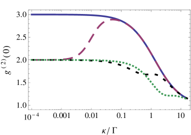
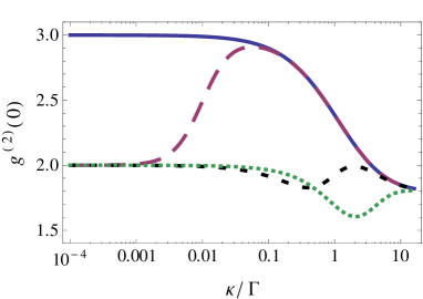
Figure 1: The steady-state dependence of the microcavity second-order photon correlation function $g^{(2)}(0)$ as a function of $\kappa/\Gamma$ for $\epsilon=0$. The solid line is for $\Delta/\Gamma=0$, the long-dashed line stands for $\Delta/\Gamma=0.01$, the short-dashed curve corresponds to $\Delta/\Gamma=1$ while the dotted line to $\Delta/\Gamma=4$. (a) N=1 while (b) N=20.

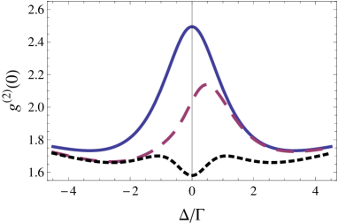
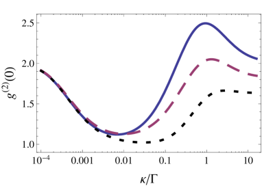
Figure 2: The steady-state dependence of the microcavity second-order photon correlation function $g^{(2)}(0)$ as a function of (a) $\Delta/\Gamma$ and (b) $\kappa/\Gamma$. The solid line is for $\phi=0$, the long-dashed line corresponds to $\phi=\pi/4$ while the short-dashed curve to $\phi=\pi/2$. Here $\epsilon/\Gamma=20$, $g/\Gamma=10$, and $N=20$. Other parameters are: (a) $\kappa/\Gamma=1$ and (b) $\Delta/\Gamma=0.01$.

III Results and Discussion

The general expression for the second-order photon correlation function is too cumbersome and, therefore, we shall represent it analytically for few particular cases. If $g_{0}=0$ one has $g^{(2)}(0)=1$ while when $\{\epsilon,\Delta\}=0$ we have:

$$g^{(2)}(0) = \frac{3(4+\kappa/\Gamma)^{2}}{(4+3\kappa/\Gamma)(6+\kappa/\Gamma)\langle R^{2}_{z}\rangle^{2}}\biggl{\{}\frac{\langle R^{4}_{z}\rangle}{1+24\Gamma/\kappa}$$

$$+ \frac{8j(j+1)\langle R^{2}_{z}\rangle}{4+\kappa/\Gamma}+\frac{16(3j(j+1)-1)\langle R^{2}_{z}\rangle}{(1+4\Gamma/\kappa)(24+\kappa/\Gamma)}\biggr{\}}.$$

One can observe here that the second-order correlation function does not depend on microcavity-dot coupling strength $g_{0}$. This is the case also for $\epsilon=0$ and $\Delta\not=0$. However, in general, i.e. when $\epsilon\not=0$, the microcavity photon correlation function depends on $g_{0}$. Note that the two-photon correlator $\langle a^{\dagger}a^{\dagger}aa\rangle\propto N^{4}$ while the photon intensity $\langle a^{\dagger}a\rangle\propto N^{2}$ and, thus, we have an enhancement of these correlations due to collectivity.

In what follows, using the system of equations (4) and for some particular cases the expression (LABEL:g20), we shall describe in details the microcavity second-order photon correlation function for various parameters of interest. We proceed by considering that the microcavity mode is not additionally pumped, i.e. $\epsilon=0$. Figure (1) shows the dependence of the second-order correlation function as a function of $\kappa/\Gamma$ for various cavity detunings and number of quantum dots involved. At the exact resonance, that is $\Delta/\Gamma=0$, one can observe larger photon correlations, i.e. $g^{(2)}(0)=3$, while their intensity is being also enhanced due to collectivity. The picture is different for the off-resonance case. As long as $\kappa\ll\Delta\not=0$ the photon statistics is similar to that of a thermal light, i.e. $g^{(2)}(0)=2$. However, for intermediate detunings one can observe a oscillatory behavior of the second-order correlation function due to the interplay of $\kappa$ and $\Gamma$. As the detuning is further increased the two-photon correlation shows a dip because of the off-resonant driving (see Fig. 1). The Fig. 1(b) does not change if one further increase the number of quantum dots.

To further understand the steady-state behaviors of the photon-photon correlation function for $\epsilon\not=0$, in Figure (2) we plot $g^{(2)}(0)$ again. However in this case, one observes a dependence of the normalized second-order correlation function $g^{(2)}(0)$ on the phase difference $\phi$ of the applied coherent sources. It is easy to show that the microcavity photon intensity (see Eqs. 4)

$$\langle a^{\dagger}a\rangle=\frac{\epsilon^{2}}{\kappa^{2}+\Delta^{2}}+\frac{(\kappa+4\Gamma)|g_{0}|^{2}\langle R^{2}_{z}\rangle}{[(\kappa+4\Gamma)^{2}+\Delta^{2}]\kappa}$$ (8)

does not depend on $\phi$ in this particular case. Therefore, the phase difference appears in the unnormalized second-order correlator $\langle a^{\dagger}a^{\dagger}aa\rangle$. This happens due to feasibility of scattering two photons from different applied coherent sources giving rise to interferences, i.e., phase dependent effects. In Fig. 2(a) one can observe an asymmetrical steady-state behavior of the second-order correlation function for $\phi=\pi/4$. Furthermore, the maximum at $\Delta/\Gamma=0$ for $\phi=0$ turns into a minimum for $\phi=\pi/2$ (see the solid and short-dashed curves in Fig. 2a, respectively). Thus, the relative phase between the applied coherent sources can be a convenient tool to manipulate the photon statistics. Particularly, one can generate coherent light, i.e. $g^{(2)}(0)\approx 1$, despite of spontaneous incoherent photon scattering into the cavity mode (see Fig. 2b). Again, the photon intensity as well as their second-order correlations are enhanced due to collectivity.

IV Summary

In summary, we have investigated the interaction of a collection of laser-pumped artificial atoms embedded in a leaking optical microcavity. Particularly, we were interested in photon statistics of the scattered photons into the cavity mode. We have found that the photon statistics depends on the phase difference between the coherent sources pumping the quantum dot system and the cavity mode, respectively. Various steady-state behaviors of photon correlations were shown to occur.

References

- (1) C. Santori and Y. Yamamoto, Nature Phys. 5, 173 (2009).
- (2) A. Muller, E. B. Flagg, P. Bianucci, X. Y. Wang, D. G. Deppe, W. Ma, J. Zhang, G. J. Salamo, M. Xiao and C. K. Shih, Phys. Rev. Lett. 99, 187402 (2007).
- (3) B. R. Mollow, Phys. Rev. 188, 1969 (1969).
- (4) A. N. Vamivakas, Y. Zhao, C.-Y. Lu and M. Atatüre, Nature Phys. 5, 198 (2009).
- (5) E. B. Flagg, A. Muller, J. W. Robertson, S. Founta, D. G. Deppe, M. Xiao, W. Ma, G. J. Salamo and C. K. Shih, Nature Phys. 5, 203 (2009).
- (6) S. M. Ulrich, S. Ates, S. Reitzenstein, A. Löffler, A. Forchel and P. Michler, Phys. Rev. Lett. 106, 247402 (2011).
- (7) A. Ulhaq, S. Weiler, S. M. Ulrich, R. Robach, M. Jetter and P. Michler, Nature Photonics 6, 238 (2012).
- (8) A. Majumdar, A. Papageorge, E. D. Kim, M. Bajcsy, H. Kim, P. Petroff and J. Vuckovic, Phys. Rev. B 84, 085310 (2011).
- (9) C. Matthiesen, A. N. Vamivakas and M. Atature, Phys. Rev. Lett. 108, 093602 (2012).
- (10) K. A. Fischer, K. Müller, A. Rundquist, T. Sarmiento, A. Y. Piggott, Y. Kelaita, C. Dory, K. G. Lagoudakis and J. Vuckovic, Nature Photonics 10, 163 (2016).
- (11) R. R. Puri Mathematical Methods of Quantum Optics (Springer, Berlin 2001), especially Chap. 12 and references therein.
- (12) C. H. Keitel, M. O. Scully and G. Süssmann, Phys. Rev. A 45, 3242 (1992).
- (13) Z. Ficek and S. Swain Quantum Interference and Coherence: Theory and Experiments (Springer, Berlin, 2005).
- (14) M. Kiffner, M. Macovei, J. Evers and C. H. Keitel, Progress in Optics 55, 85 (2010).
- (15) S. Ya. Kilin, Sov. Phys. JETP 51, 1081 (1980).
- (16) P. Longo and J. Evers, Phys. Rev. Lett. 112, 193601 (2014).
- (17) M. Scheibner, T. Schmidt, L. Worschech, A. Forchel, G. Bacher, T. Passow and D. Hommel, Nature Phys. 3, 106 (2007).
- (18) V. I. Yukalov and E. P. Yukalova, Phys. Rev. B 81, 075308 (2010).
- (19) A. Sitek and P. Machnikowski, Phys. Rev. B 75, 035328 (2007).
- (20) M. Macovei and C. H. Keitel, Phys. Rev. B 75, 245325 (2007).
- (21) A. Sitek and A. Manolescu, Phys. Rev. B 88, 043807 (2013).
- (22) H. A. M. Leymann, A. Foerster, F. Jahnke, J. Wiersig and C. Gies, Phys. Rev. Applied 4, 044018 (2015).
- (23) N. S. Averkiev, M. M. Glazov and A. N. Poddubnyi, JETP 108, 836 (2009).
- (24) G.-x. L, Y.-p. Yang, K. Allaart and D. Lenstra, Phys. Rev. A 69, 014301 (2004).
- (25) C. H. Keitel, Phys. Rev. Lett. 83, 1307 (1999).