Effects of losses in the hybrid atom-light interferometer

Abstract

Enhanced Raman scattering can be obtained by injecting a seeded light field which is correlated with the initially prepared collective atomic excitation. This Raman amplification process can be used to realize atom-light hybrid interferometer. We numerically calculate the phase sensitivities and the signal-to-noise ratios of this interferometer with the method of homodyne detection and intensity detection, and give their differences between this two methods. In the presence of loss of light field and atomic decoherence the measure precision will be reduced which can be explained by the break of the intermode decorrelation conditions of output modes.

I Introduction

Quantum parameter estimation is the use of quantum techniques to improve measurement precision than purely classical approaches, which has been received a lot of attention in recent years Helstrom76 ; Holevo82 ; Caves81 ; Braunstein94 ; Braunstein96 ; Lee02 ; Giovannetti06 ; Zwierz10 ; Giovannetti04 ; Giovannetti11 ; Ou . Interferometers can provide the most precise measurements. Recently, physicists with the advanced Laser Interferometer Gravitational-Wave Observatory (LIGO) observed the gravitational waves Abbott . The Mach–Zehnder interferometer (MZI) and its variants have been used as a generic model to realize precise measurement of phase. In order to avoid the vacuum fluctuations enter the unused port and are amplified in the interferometer by the coherent light, Caves Caves81 suggested to replace the vacuum fluctuations with the squeezed-vacuum light to reach a sub-shot-noise sensitivity. Xiao et al. Xiao and Grangier et al. Grangier  have demonstrated the experimental results beyond the standard quantum limit (SQL) $\delta\varphi=1/\sqrt{N}$ with $N$ number of photons or other bosons. Due to overcoming the SQL and reaching the Heisenberg limit (HL) $\delta\varphi=1/N$, it will lead to potential applications in high resolution measurements. Therefore, many theoretical proposals and experimental techniques are developed to improve the sensitivity Toth ; PezzBook ; Demkowicz . When the probe states made of correlated states, such as the NOON states of the form $(|N\rangle_{a}|0\rangle_{b}+e^{i\phi_{N}}|0\rangle_{a}|N\rangle_{b})/\sqrt{2}$, the HL in the phase-shift measurements can reach Dowling08 ; NOON . But, high-$N$ NOON states is very hard to synthesize. In the presence of realistic imperfections and noise, the ultimate precision limit in noisy quantum-enhanced metrology was also studied Dem09 ; Escher ; Dem12 ; Berry13 ; Chaves ; Dur ; Kessler ; Alipour .

However, most of the current atomic and optical interferometers are made of linear devices such as beam splitters and phase shifters. In 1986, Yurke et al. Yurke86 introduced a new interferometer where two nonlinear beam splitters take the place of two linear beam splitters (BSs) in the traditional MZI. It is also called the SU(1,1) interferometer because it is described by the SU(1,1) group, as opposed to SU(2) for BSs. The detailed quantum statistics of the two-mode SU(1,1) interferometer was studied by Leonhardt Leonhardt . SU(1,1) phase states also have been studied theoretically in quantum measurements for phase-shift estimation Vourdas ; Sanders . An improved theoretical scheme of the SU(1,1) optical interferometer was presented by Plick et al Plick who proposed to inject a strong coherent beam to “boost” the photon number. Experimental realization of this SU(1,1) optical interferometer was reported by different groups Jing11 ; Lett . The noise performance of this interferometer was analyzed Marino ; Ou and under the same phase-sensing intensity condition the improvement of $4.1$ dB in signal-to-noise ratio was observed Hudelist . By contrast, SU(1,1) atomic interferometer also has been experimentally realized with Bose-Einstein Condensates Gross ; Linnemann ; Peise ; Gabbrielli . Gabbrielli et al. Gabbrielli realized a nonlinear three-mode SU(1,1) atomic interferometer, where the analogy of optical down conversion, the basic ingredient of SU(1,1) interferometry, is created with ultracold atoms.

Collective atomic excitation due to its potential applications for quantum information processing has attracted a great deal of interest Duan ; Polzik ; Kuzmich . Collective atomic excitation can be realized by the Raman scattering. Initially prepared collective atomic excitation can be used to enhance the second Raman scattering Chen09 ; Chen10 ; Yuan10 . Subsequently, we proposed another scheme to enhance the Raman scattering using the correlation-enhanced mechanism Yuan13 . That is, by injecting a seeded light field which is correlated with the initially prepared collective atomic excitation, the Raman scattering can be enhanced greatly, which was also realized in experiment recently Chen15 . Such a photon-atom interface can form an SU(1,1)-typed atom-light hybrid interferometer ChenPRL15 , where the atomic Raman amplification processes replacing the beam splitting elements in a traditional MZI Yurke86 . Different from all-optical or all-atomic interferometers, the atom-light hybrid interferometers depend on both atomic and optical phases so that we can probe the atomic phases with optical interferometric techniques. The atomic phase can be adjusted by magnetic field or Stark shifts. The atom-light hybrid interferometer is composed of two Raman amplification processes. The first nonlinear process generates the correlated optical and atomic waves in the two arms and they are decorrelated by the second nonlinear process.

In this paper, we calculate the phase sensitivities and the SNRs using the homodyne detection and the intensity detection. The differences between the phase sensitivities and the SNRs are compared. The loss of light field and atomic decoherence will degrade the measure precision. The effects of the light field loss and atomic decoherence on measure precision can be explained from the break of intermode decorrelation conditions.

Our article is organized as follows. In Sec. II, we give the model of the hybrid atom-light interferometer, and in Sec. III we numerically calculate the phase sensitivity and the SNR, and analyze and compare the conditions to obtain the optimal phase sensitivity and the maximal SNR. In Sec. IV, the LCCs of the amplitude quadrature and number operator are derived from the light-atom coupling equations in the presence of light field loss and atomic decoherence. The LCCs as a function of the transmission rate and the collisional rate are calculated and analyzed. The loss of light field and atomic decoherence will degrade the measure precision, which is explained from the intermode decorrelation conditions break. Finally, in Sec. V we conclude with a summary of our results.

II The Model of atom-light hybrid interferometer

Figure 1: (Color online) (a) The intermode correlation between the Stokes field $\hat{a}_{1}$ and the atomic excitation $\hat{b}_{1}$ is generated by spontaneous Raman process. $\hat{a}_{0}$ is the initial input light field. $\hat{b}_{0}$ is in vacuum or an initial atomic collective excitation which can be prepared by another Raman process or electromagnetically induced transparency process. (b) During the delay time $\tau$, the Stokes field $\hat{a}_{1}$ will be subject to the photon loss and evolute to $\hat{a}^{\prime}_{1}$ and the collective excitation $\hat{b}_{1}$ will undergo the collisional dephasing to $\hat{b}^{\prime}_{1}$. A fictitious beam splitter (BS) is introduced to mimic the loss of photons into the environment. $\hat{V}$ is the vacuum. (c) After the delay time $\tau$, the light field $\hat{a}^{\prime}_{1}$ and its correlated atomic excitation $\hat{b}^{\prime}_{1}$ are used as initial seeding for another enhanced Raman process. (d)-(f) The corresponding energy-level diagrams of different processes are shown.

In this section, we review the different processes of the atom-light interferometer ChenPRL15 ; Ma as shown in Fig. 1(a)-(c), where two Raman systems replaced the BSs in the traditional MZI. Considering a three-level Lambda-shaped atom system as shown in Fig. 1(d), the Raman scattering process is described by the following pair of coupled equations Raymer04 :

$$\frac{\partial\hat{a}(t)}{\partial t}=\eta A_{P}\hat{b}^{{\dagger}}(t),\text{ \ \ }\frac{\partial\hat{b}(t)}{\partial t}=\eta A_{P}\hat{a}^{{\dagger}}(t),$$ (1)

where $\eta$ is the coupling constant, and $A_{P}$ is the amplitude of the pump field. The solution of above equation is

$$\hat{a}(t)=u(t)\hat{a}(0)+v(t)\hat{b}^{{\dagger}}(0),\text{ }\hat{b}(t)=u(t)\hat{b}(0)+v(t)\hat{a}^{{\dagger}}(0),$$ (2)

where $u(t)=\cosh(g)$, $v(t)=e^{i\theta}\sinh(g)$, $g=\left|\eta A_{P}\right|t$, $e^{i\theta}=(A_{P}/A_{P}^{\ast})^{1/2}$, and $t$ is the time duration of pump field $E_{P}$. We use different subscripts to differentiate the two processes, where $1$ denotes the first Raman process (RP1) and $2$ denotes the second Raman process (RP2). $t_{1}$ and $t_{2}$ are the durations of the pump field $E_{P1}$ and $E_{P2}$, respectively.

After the first Raman process of the interferometer, the Stokes field $\hat{a}_{1}$ and the atomic excitation $\hat{b}_{1}$ are generated as shown in Fig. 1(a). Then after a small delay time $\tau$, the second Raman process of the interferometer takes place which is used as beams combination as shown in Fig. 1(c). During the small delay time $\tau$ shown in Fig. 1(b), the Stokes field $\hat{a}_{1}$ will be subject to the photon loss and evolute to $\hat{a}_{1}^{\prime}$ . A fictitious BS is introduced to mimic the loss of photons into the environment, then the light field $\hat{a}_{1}^{\prime}$ is given by

$$\hat{a}_{1}^{\prime}=\sqrt{T}\hat{a}_{1}(t_{1})e^{i\phi}+\sqrt{R}\hat{V},$$ (3)

where $T$ and $R$ are the transmission and reflectance coefficients with $T+R=1$, and $\hat{V}$ is in vacuum. The collective excitation $\hat{b}_{1}$ will also undergo the collisional dephasing described by the factor $e^{-\Gamma\tau}$, then $\hat{b}_{1}^{\prime}$ is

$$\hat{b}_{1}^{\prime}=\hat{b}_{1}(t_{1})e^{-\Gamma\tau}+\hat{F},$$ (4)

where $\hat{F}=\int_{0}^{\tau}e^{-\Gamma(\tau-t^{\prime})}\hat{f}(t^{\prime})dt^{\prime}$, and $\hat{f}(t)$ is the quantum statistical Langevin operator describing the collision-induced fluctuation, and obeys $\langle\hat{f}(t)\hat{f}^{{\dagger}}(t^{\prime})\rangle=2\Gamma\delta(t-t^{\prime})$ and $\langle\hat{f}^{{\dagger}}(t)\hat{f}(t^{\prime})\rangle=0$. Then $\langle\hat{F}\hat{F}^{{\dagger}}\rangle=1-e^{-2\Gamma\tau}$ guarantees the consistency of the operator properties of $\hat{b}_{1}^{\prime}$.

Using Eqs. (2)-(4), the generated Stokes field $\hat{a}_{2}$ and collective atomic excitation $\hat{b}_{2}$ can be worked out:

$$\hat{a}_{2}(t_{2}) =\mathcal{U}_{1}\hat{a}_{1}(0)+\mathcal{V}_{1}\hat{b}_{1}^{{\dagger}}(0)+\sqrt{R}u_{2}\hat{V}+v_{2}\hat{F}^{{\dagger}},$$ (5)

$$\hat{b}_{2}(t_{2}) =e^{-i\phi}[\mathcal{U}_{2}\hat{b}_{1}(0)+\mathcal{V}_{2}\hat{a}_{1}^{{\dagger}}(0)]+\sqrt{R}v_{2}\hat{V}^{{\dagger}}+u_{2}\hat{F},$$ (6)

where

$$\mathcal{U}_{1} =\sqrt{T}u_{1}u_{2}e^{i\phi}+e^{-\Gamma\tau}v_{1}^{\ast}v_{2},\text{ }\mathcal{V}_{1}=\sqrt{T}v_{1}u_{2}e^{i\phi}$$

$$+e^{-\Gamma\tau}u_{1}^{\ast}v_{2},\text{ }\mathcal{U}_{2}=e^{-\Gamma\tau}u_{1}u_{2}e^{i\phi}$$

$$+\sqrt{T}v_{1}^{\ast}v_{2},\text{ }\mathcal{V}_{2}=e^{-\Gamma\tau}v_{1}u_{2}e^{i\phi}+\sqrt{T}u_{1}^{\ast}v_{2}.$$ (7)

Next, we use the above results to calculate the phase sensitivity and the SNR, and analyze and compare the conditions to obtain optimal phase sensitivity and the maximal SNR.

III Phase sensitivity and SNR

Figure 2: (Color online) The phase sensitivity $\Delta\phi_{\mathrm{HD}}$ and the $\mathrm{SNR_{HD}}$ versus the phase shift $\phi$ using the method of homodyne detection with (a) $\theta_{\alpha}=\pi/2$; (b) $\theta_{\alpha}=0$. Parameters: $g=2$, $|\alpha|=10$.

Phase can be estimated but cannot be measured because there is not a Hermitian operator corresponding to a quantum phase Lynch . In phase precision measurement, the estimation of a phase shift can be done by choosing an observable, and the the relationship between the observable and the phase is known. The mean-square error in parameter $\phi$ is then given by the error propagation formula Dowling08 :

$$\Delta\phi=\frac{\langle(\Delta\hat{O})^{2}\rangle^{1/2}}{\left|\partial\langle\hat{O}\rangle/\partial\phi\right|},$$ (8)

where $\hat{O}$ is the measurable operator and $\langle(\Delta\hat{O})^{2}\rangle=\langle\hat{O}^{2}\rangle-\langle\hat{O}\rangle^{2}$. The precision of the phase shift measurement is not the only parameter of concern. We also need consider the SNR Kim ; Ou ; Barzanjeh , which is given by

$$\text{SNR}=\frac{\langle\hat{O}\rangle}{\langle(\Delta\hat{O})^{2}\rangle^{1/2}}.$$ (9)

In current optical measurement of phase sensitivity, the homodyne detection Ole ; Li14 ; Barzanjeh and the intensity detection Plick ; Marino are often used. That is, the observables are the amplitude quadrature operator $\hat{x}_{a2}=(\hat{a}_{2}+\hat{a}_{2}^{\dagger})/2$ and the number operator $\hat{n}_{a2}=\hat{a}_{2}^{\dagger}\hat{a}_{2}$. For the balanced situation that is $g_{1}=g_{2}=g$, and $\theta_{2}-\theta_{1}=\pi$. Firstly, we do not consider the effect of loss on the generated Stokes field $\hat{a}_{2}$ and atomic collective excitation $\hat{b}_{2}$. That is, $R=0$ and $\Gamma\tau=0$, it reduced to the ideal lossless case and we have $\mathcal{U}_{1}=\mathcal{U}_{2}=\mathcal{U}=[\cosh^{2}ge^{i\phi}-\sinh^{2}g]$, $\mathcal{V}_{1}=\mathcal{V}_{2}=\mathcal{V}=\frac{1}{2}\sinh 2g[e^{i\phi}-1]e^{i\theta_{1}}$, where $\left|\mathcal{U}\right|^{2}-\left|\mathcal{V}\right|^{2}=1$.

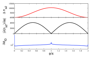
Figure 3: (Color online) (a) $\Delta{n}_{a2}$, $|\langle\partial\langle{n}_{a2}\rangle/\partial\phi\rangle|$, and the phase sensitivity $\Delta\phi_{\mathrm{ID}}$; (b) $\langle{n}_{a2}\rangle$, $\Delta{n}_{a2}$ and the $\mathrm{SNR_{ID}}$ versus the phase shift $\phi$ using the method of intensity detection. Parameters: $g=2$, $|\alpha|=10$.

III.1 Homodyne detection

For a coherent light $|\alpha\rangle$ ($\alpha=\left|\alpha\right|e^{i\theta_{\alpha}}$, $N_{\alpha}=\left|\alpha\right|^{2}$) as the phase-sensing field, using the amplitude quadrature operator $\hat{x}_{a2}$ as the detected variable the phase sensitivity and the SNR are given by

$$\Delta\phi_{\text{HD}} =\frac{\langle(\Delta\hat{x}_{a2})^{2}\rangle^{1/2}}{\sqrt{N_{\alpha}}\cosh^{2}g\left|\sin(\phi+\theta_{\alpha})\right|},$$ (10)

$$\text{SNR}_{\text{HD}} =\frac{\sqrt{N_{\alpha}}[\cosh^{2}g\cos(\phi+\theta_{\alpha})-\sinh^{2}g\cos(\theta_{\alpha})]}{\langle(\Delta\hat{x}_{a2})^{2}\rangle^{1/2}},$$ (11)

with

$$\langle(\Delta\hat{x}_{a2})^{2}\rangle=\frac{1}{4}\left[\cosh^{2}(2g)-\sinh^{2}(2g)\cos\phi\right],$$ (12)

where the subscript HD denotes the homodyne detection. The phase sensitivity $\Delta\phi_{\text{HD}}$ and the SNR${}_{\text{HD}}$ depend on $\phi$ and $\theta_{\alpha}$, when $g$ and $\alpha$ take a certain values. From Eqs. (10) and (11), both the $\Delta\phi_{\text{HD}}$ and the SNR${}_{\text{HD}}$ need that the term $\langle(\Delta\hat{x}_{a2})^{2}\rangle$ is minimal, which can be realized at $\phi=0$ and $\langle(\Delta\hat{x}_{a2})^{2}\rangle=1/4$ Scully .

When $\phi=0$ and $\theta_{\alpha}=\pi/2$, we obtain the optimal phase sensitivity and the worst SNR:

$$\Delta\phi_{\text{HD}} =\frac{1}{\sqrt{N_{\alpha}}}\frac{1}{2\cosh^{2}g},$$ (13)

$$\text{SNR}_{\text{HD}} =0.$$ (14)

But when $\phi=0$ and $\theta_{\alpha}=0$ or $\pi$, the maximal SNR${}_{\text{HD}}$ is given by

$$\text{SNR}_{\text{HD}}=2\sqrt{N_{\alpha}},$$ (15)

and the sensitivity $\Delta\phi_{\text{HD}}$ is divergent. The phase sensitivity $\Delta\phi_{\text{HD}}$ and the SNR${}_{\text{HD}}$ of above two different cases are shown in Figs. 2(a) and 2(b), respectively. We find that at the optimal point $\phi=0$ and $\theta_{\alpha}=\pi/2$ the sensitivity is high (i.e. $\Delta\phi$ small) and can beat the SQL but the SNR${}_{\text{HD}}$ is low. At the optimal point $\phi=0$ and $\theta_{\alpha}=0$ the SNR${}_{\text{HD}}$ is high, but the sensitivity is low. Ideally, of course, we would like high sensitivity $\Delta\phi_{\text{HD}}$ and high SNR${}_{\text{HD}}$ at the same optimal point.

III.2 Intensity detection

Figure 4: (Color online) The phase sensitivities $\Delta\phi$ versus the phase-sensing probe number $n_{\mathrm{ph}}$. The optimal phase sensitivities $\Delta\phi_{\text{HD}}$ and $\Delta\phi_{\text{ID}}$ are obtained at $\phi=0$ and $\phi=0.062$, respectively. Parameter: $g=2$.

If we use $\hat{n}_{a2}$ ($=\hat{a}_{2}^{\dagger}\hat{a}_{2}$) as the detection variable, for a coherent light $|\alpha\rangle$ ($\alpha=\left|\alpha\right|e^{i\theta_{\alpha}}$, $N_{\alpha}=\left|\alpha\right|^{2}$) as the phase-sensing field, the phase sensitivity and the SNR are given by

$$\Delta\phi_{\text{ID}} =\langle(\Delta\hat{n}_{a2})^{2}\rangle^{1/2}\frac{2}{(N_{\alpha}+1)\sinh^{2}(2g)\left|\sin\phi\right|},$$ (16)

$$\text{SNR}_{\text{ID}} =\frac{1}{\langle(\Delta\hat{n}_{a2})^{2}\rangle^{1/2}}[N_{\alpha}\left|\cosh^{2}g-\sinh^{2}ge^{-i\phi}\right|^{2}$$

$$+\frac{1}{2}\sinh^{2}(2g)(1-\cos\phi)],$$ (17)

where the subscript ID denotes the intensity detection, and

$$\langle(\Delta\hat{n}_{a2})^{2}\rangle=N_{\alpha}\left|\cosh^{2}g-\sinh^{2}ge^{-i\phi}\right|^{4}+\frac{1}{2}\left(1+N_{\alpha}\right)$$

$$\times\sinh^{2}(2g)\left|\cosh^{2}g-\sinh^{2}ge^{-i\phi}\right|^{2}(1-\cos\phi).$$ (18)

Different from the homodyne detection, the phase sensitivity $\Delta\phi_{\text{ID}}$ and the SNR${}_{\text{ID}}$ only depend on $\phi$ for given $g$ and $N_{\alpha}$. Under the condition of $g=2$ and $N_{\alpha}=\sqrt{10}$, the phase sensitivity $\Delta\phi_{\text{ID}}$ and the SNR${}_{\text{ID}}$ as a function of phase shift $\phi$ are shown in Figs. 3(a) and 3(b), respectively. The best phase sensitivity $\Delta\phi_{\text{ID}}$ and the maximal SNR${}_{\text{ID}}$ ($=\sqrt{N_{\alpha}}$) are obtained at $\phi\approx 0.062$ and $\phi=0$, respectively. In Fig. 3(a) at $\phi\approx 0$ the slope $\left|\partial\langle\hat{n}_{a2}\rangle/\partial\phi\right|$ is very small, as well in Fig. 3(b) at $\phi=0$ the intensity of the signal $\langle\hat{n}_{a2}\rangle$ is low, but the noise is also low. It demonstrated that the noise $\langle(\Delta\hat{n}_{a2})^{2}\rangle$ plays a dominant role. The best phase sensitivity from the intensity detection is lower than it from the homodyne detection, i.e., $\Delta\phi_{\text{ID}}>\Delta\phi_{\text{HD}}$. The relation of maximal SNR from two detection methods is SNR${}_{\text{HD}}=2$SNR${}_{\text{ID}}$.

III.3 Losses case

If the presence of loss of light field and atomic decoherence, the precision of the sensitivity and the SNR will be reduced Li14 ; Ma . According to the linear error propagation, the mean-square error in parameter $\phi$ is given by

$$\Delta\phi=\frac{\langle(\Delta\hat{O})^{2}\rangle^{1/2}}{\left|\partial\langle\hat{O}\rangle/\partial\phi\right|}.$$

The slopes of the output amplitude quadrature operator $\hat{X}_{a2}$ and the number operator $\hat{n}_{a2}=\hat{a}_{2}^{\dagger}\hat{a}_{2}$ are respectively given by

$$\left|\frac{\partial\langle\hat{X}_{a2}\rangle}{\partial\phi}\right| =\sqrt{TN_{\alpha}}\cosh^{2}g\left|\sin(\phi+\theta_{\alpha})\right|,$$ (19)

$$\left|\frac{\partial\langle\hat{n}_{a}\rangle}{\partial\phi}\right| =\frac{1}{2}\sqrt{T}e^{-\Gamma\tau}(N_{\alpha}+1)\sinh^{2}(2g)\left|\sin(\phi)\right|.$$ (20)

The uncertainties of the output amplitude quadrature operator $\hat{X}_{a2}$ and the number operator$\ \hat{n}_{a2}$ are given by

$$\langle(\Delta\hat{X}_{a2})^{2}\rangle =\frac{1}{4}[\sinh^{2}(2g)(T/2-\sqrt{T}e^{-\Gamma\tau}\cos\phi)$$

$$+2e^{-2\Gamma\tau}\sinh^{4}g+\cosh(2g)],$$ (21)

$$\langle(\Delta\hat{n}_{a2})^{2}\rangle =\left|\mathcal{U}_{b}\right|^{4}\left|\alpha\right|^{2}+\left|\mathcal{U}_{b}\mathcal{V}_{b}\right|^{2}(1+\left|\alpha\right|^{2})$$

$$+R\cosh^{2}g(\left|\mathcal{U}_{b}\right|^{2}\left|\alpha\right|^{2}+\left|\mathcal{V}_{b}\right|^{2})$$

$$+\sinh^{2}g [\left|\mathcal{U}_{b}\right|^{2}(1+\left|\alpha\right|^{2})+R\cosh^{2}g](1-e^{-2\Gamma\tau}),$$ (22)

where

$$\left|\mathcal{U}_{b}\right|^{2} =(\sqrt{T}\cosh^{2}g+e^{-\Gamma\tau}\sinh^{2}g)^{2}$$

$$-2\sqrt{T}e^{-\Gamma\tau}\sinh^{2}g\cosh^{2}g(1+\cos\phi),$$

$$\left|\mathcal{V}_{b}\right|^{2} =\frac{1}{2}\sinh^{2}(2g)(T+e^{-2\Gamma\tau}-2\sqrt{T}e^{-\Gamma\tau}\cos\phi).$$ (23)

The subscript $b$ denotes the balanced condition when considering the losses case.

The phase sensitivities $\Delta\phi$ as a function of the phase-sensing probe number $n_{\text{ph}}$ is shown in Fig. 4. The thick solid line is the SQL. The thin solid line and dotted line are sensitivities $\Delta\phi_{\text{HD}}$ from homodyne detection with and without losses cases, respectively. As well the dashed and dash-dotted lines are sensitivities $\Delta\phi_{\text{ID}}$ from intensity detection with and without losses cases, respectively. From Fig. 4, it is easy to see that the best phase sensitivities $\Delta\phi_{\text{ID}}$ are larger than $\Delta\phi_{\text{HD}}$ under the same condition. In the presence of the loss and collisional dephasing ($T=0.8$, $\Gamma\tau=0.1$), the phase sensitivities $\Delta\phi_{\text{HD}}$ and $\Delta\phi_{\text{ID}}$ can beat the SQL under the balanced situation, which is very important for phase sensitivity measurement.

Next section, we explain the reason that the effects of the light field loss and atomic decoherence on measure precision can be explained from the break of intermode decorrelation conditions.

IV The correlations of atom-light hybrid interferometer

In this section, we use the above results to calculate the intermode correlations of the different Raman amplification processes of the atom-light interferometer as shown in Fig. 1(a)-(c) ChenPRL15 . We also study the effects of the loss of light field and the dephasing of atomic excitation on the correlation. The intermode correlation of light and atomic collective excitation can be described by the linear correlation coefficient (LCC), which is defined as Gerry

$$J(\hat{A},\hat{B})=\frac{cov(\hat{A},\hat{B})}{\langle(\Delta\hat{A})^{2}\rangle^{1/2}\langle(\Delta\hat{B})^{2}\rangle^{1/2}},$$ (24)

where $cov(\hat{A},\hat{B})=(\langle\hat{A}\hat{B}\rangle+\langle\hat{B}\hat{A}\rangle)/2-\langle\hat{A}\rangle\langle\hat{B}\rangle$ is the covariance of two-mode field and $\langle(\Delta\hat{A})^{2}\rangle=\langle\hat{A}^{2}\rangle-\langle\hat{A}\rangle^{2}$, $\langle(\Delta\hat{B})^{2}\rangle=\langle\hat{B}^{2}\rangle-\langle\hat{B}\rangle^{2}$.

The respective quadrature operators of the light and atomic excitation are $\hat{x}_{a}=(\hat{a}+\hat{a}^{\dagger})/2$, $\hat{y}_{a}=(\hat{a}-\hat{a}^{\dagger})/2i$, $\hat{x}_{b}=(\hat{b}+\hat{b}^{\dagger})/2$, and $\hat{y}_{b}=(\hat{b}-\hat{b}^{\dagger})/2i$. After the first Raman scattering process, the intermode correlations between the light field mode and the atomic mode are generated. We start by injecting a coherent state $|\alpha\rangle$ in mode $\hat{a}$, and a vacuum state in mode $\hat{b}$, the LCC of quadratures are given by

$$J_{x1}(\hat{x}_{a1},\hat{x}_{b1}) =\cos\theta_{1}\tanh(2g_{1}),$$ (25)

$$J_{y1}(\hat{y}_{a1},\hat{y}_{b1}) =-\cos\theta_{1}\tanh(2g_{1}),$$ (26)

and the LCC of number operators $\hat{n}_{a1}$ $[=\hat{a}^{{\dagger}}(t_{1})\hat{a}(t_{1})]$ and $\hat{n}_{b1}$ $[=\hat{b}^{{\dagger}}(t_{1})\hat{b}(t_{1})]$ is given by

$$J_{n1}(\hat{n}_{a1},\hat{n}_{b1})=\frac{(1+2\left|\alpha\right|^{2})}{[4\coth^{2}(2g_{1})(\left|\alpha\right|^{2}+\left|\alpha\right|^{4})+1]^{1/2}}.$$ (27)

From Eqs. (25)-(27), the quadrature correlation LCCs $J_{x1}(\hat{x}_{a1},\hat{x}_{b1})$ and $J_{y1}(\hat{y}_{a1},\hat{y}_{b1})$ are independent on the input coherent state which is different from the number correlation LCC $J_{n1}(\hat{n}_{a1},\hat{n}_{b1})$. Under $\theta_{1}\neq\pi/2$, the LCCs $J_{x1}$ and $J_{y1}$ are opposite and not zero, which shows the correlation exists. Due to their opposite intermode correlations, the squeezing of quantum fluctuations is in a superposition of the two-modes, i.e., $\hat{X}=(\hat{x}_{a}+\hat{x}_{b})/\sqrt{2}$, $\hat{Y}=(\hat{y}_{a}+\hat{y}_{b})/\sqrt{2}$ and $[\hat{X},\hat{Y}]=i/2$ Gerry .

From Eq. (27) the number correlation LCC $J_{n1}$ is always positive so long as$\ g\neq 0$. If $\alpha=0$, that is vacuum state input, then $J_{n1}(\hat{n}_{a1},\hat{n}_{b1})=1$, this maximal value shows the strong intermode correlation and such states in optical fields are often called ”twin beams”. For this vacuum state input case, the state of atomic mode and light mode is similar to the two-mode squeezed vacuum state.

Figure 5: (Color online) The linear correlation coefficients (a) $J_{x2}$; (b) $J_{n2}$ as a function of the phase shift $\phi$ for lossless case. Parameters: $\theta_{1}=0$, $g=2$, $|\alpha|=10$.

Figure 6: (Color online) The linear correlation coefficients $J_{x2}$ as a function of (a) the transmission rate $T$; (b) the collisional rate $\Gamma\tau$. Parameters: $g=2$, $|\alpha|=10$, $\theta_{\alpha}=\pi/2$ and $\phi=0$.

After the second Raman process of the interferometer, the LCC of quadratures $J_{x2}(\hat{x}_{a2},\hat{x}_{b2})$ using the generated Stokes field $\hat{a}_{2}$ and atomic collective excitation $\hat{b}_{2}$ can be worked out

$$J_{x2}(\hat{x}_{a2},\hat{x}_{b2})=\frac{cov(\hat{x}_{a2},\hat{x}_{b2})}{\langle(\Delta\hat{x}_{a2})^{2}\rangle^{1/2}\langle(\Delta\hat{x}_{b2})^{2}\rangle^{1/2}},$$ (28)

where

$$cov(\hat{x}_{a2},\hat{x}_{b2})=\frac{1}{4}\mathrm{Re}[e^{-i\phi}(\mathcal{V}_{1}\mathcal{U}_{2}+\mathcal{U}_{1}\mathcal{V}_{2})+u_{2}v_{2}$$

$$\times(R+1-e^{-2\Gamma\tau})],$$

$$\langle(\Delta\hat{x}_{a2})^{2}\rangle=\frac{1}{4}[\left|\mathcal{U}_{1}\right|^{2}+\left|\mathcal{V}_{1}\right|^{2}+R\left|u_{2}\right|^{2}+\left|v_{2}\right|^{2}(1-e^{-2\Gamma\tau})],$$

$$\langle(\Delta\hat{x}_{b2})^{2}\rangle=\frac{1}{4}[\left|\mathcal{U}_{2}\right|^{2}+\left|\mathcal{V}_{2}\right|^{2}+R\left|v_{2}\right|^{2}+\left|u_{2}\right|^{2}(1-e^{-2\Gamma\tau})].$$ (29)

The LCC of number operators $J_{n2}(\hat{n}_{a2},\hat{n}_{b2})$ can also be worked out

$$J_{n2}(\hat{n}_{a2},\hat{n}_{b2})=\frac{cov(\hat{n}_{a2},\hat{n}_{b2})}{\langle(\Delta\hat{n}_{a2})^{2}\rangle^{1/2}\langle(\Delta\hat{n}_{b2})^{2}\rangle^{1/2}},$$ (30)

where

$$cov(\hat{n}_{a2},\hat{n}_{b2})=\left|\mathcal{U}_{1}\mathcal{V}_{2}\right|^{2}\left|\alpha\right|^{2}+(1+\left|\alpha\right|^{2})\operatorname{Re}[\mathcal{U}_{1}^{\ast}\mathcal{U}_{2}\mathcal{V}_{1}\mathcal{V}_{2}^{\ast}]$$

$$+(1-e^{-2\Gamma\tau})(R\left|u_{2}v_{2}\right|^{2}+(1+\left|\alpha\right|^{2})\operatorname{Re}[e^{i\phi}\mathcal{U}_{1}^{\ast}\mathcal{V}_{2}^{\ast}u_{2}v_{2}])$$

$$+R\operatorname{Re}[e^{-i\phi}\mathcal{U}_{2}\mathcal{V}_{1}u_{2}^{\ast}v_{2}^{\ast}]+R\left|\alpha\right|^{2}\operatorname{Re}[e^{-i\phi}\mathcal{U}_{1}\mathcal{V}_{2}u_{2}^{\ast}v_{2}^{\ast}],$$ (31)

$$\langle(\Delta\hat{n}_{a2})^{2}\rangle=\left|\mathcal{U}_{1}\right|^{4}\left|\alpha\right|^{2}+\left|\mathcal{U}_{1}\mathcal{V}_{1}\right|^{2}(1+\left|\alpha\right|^{2})+R\left|\mathcal{V}_{1}u_{2}\right|^{2}$$

$$+R\left|\mathcal{U}_{1}u_{2}\right|^{2}\left|\alpha\right|^{2}+\left|\mathcal{U}_{1}v_{2}\right|^{2}(1-e^{-2\Gamma\tau})\left|\alpha\right|^{2}$$

$$+(\left|\mathcal{U}_{1}v_{2}\right|^{2}+R\left|u_{2}v_{2}\right|^{2})(1-e^{-2\Gamma\tau}),$$ (32)

$$\langle(\Delta\hat{n}_{b2})^{2}\rangle=\left|\mathcal{V}_{2}\right|^{4}\left|\alpha\right|^{2}+\left|\mathcal{U}_{2}\mathcal{V}_{2}\right|^{2}(1+\left|\alpha\right|^{2})+R\left|\mathcal{U}_{2}v_{2}\right|^{2}$$

$$+R\left|\mathcal{V}_{2}v_{2}\right|^{2}\left|\alpha\right|^{2}+\left|\mathcal{V}_{2}u_{2}\right|^{2}(1-e^{-2\Gamma\tau})\left|\alpha\right|^{2}$$

$$+(\left|\mathcal{V}_{2}u_{2}\right|^{2}+R\left|u_{2}v_{2}\right|^{2})(1-e^{-2\Gamma\tau}).$$ (33)

Firstly, we do not consider the effect of loss on the generated Stokes field $\hat{a}_{2}$ and atomic collective excitation $\hat{b}_{2}$. Under this ideal and balanced conditions, the LCCs of quadratures and number operators are respectively given by

$$J_{x2} (\hat{x}_{a2},\hat{x}_{b2})=\frac{2\mathrm{Re}[\mathcal{VU}e^{i\phi}]}{\left|\mathcal{U}\right|^{2}+\left|\mathcal{V}\right|^{2}}$$

$$=\frac{\sinh(2g)}{\cosh^{2}(2g)-\sinh^{2}(2g)\cos\phi}[\cosh^{2}g\cos(\theta_{1}+3\phi)$$

$$+\sinh^{2}g\cos(\theta_{1}+\phi)-\cosh(2g)\cos(\theta_{1}+2\phi)],$$ (34)

and

$$J_{n2}(\hat{n}_{a2},\hat{n}_{b2})=\frac{\left|\mathcal{UV}\right|(1+2\left|\alpha\right|^{2})}{(\mathcal{\bar{U}\bar{V}})^{1/2}}=(1+2\left|\alpha\right|^{2})$$

$$\times\left[\frac{4\left[1+\sinh^{2}(2g)(1-\cos\phi)\right]^{2}(\left|\alpha\right|^{2}+\left|\alpha\right|^{4})}{[1+\sinh^{2}(2g)(1-\cos\phi)]^{2}-1}+1\right]^{-1/2},$$ (35)

where $\mathcal{\bar{U}}=\left|\mathcal{U}\right|^{2}\left|\alpha\right|^{2}+\left|\mathcal{V}\right|^{2}(\left|\alpha\right|^{2}+1)$, $\mathcal{\bar{V}}=\left|\mathcal{V}\right|^{2}\left|\alpha\right|^{2}+\left|\mathcal{U}\right|^{2}(\left|\alpha\right|^{2}+1)$. When the phase shift $\phi$ is 0, $\mathcal{V}$ is also equal to $0$, then the LCC $J_{x2}(\hat{x}_{a2},\hat{x}_{b2})$ and $J_{n2}(\hat{n}_{a2},\hat{n}_{b2})$ are $0$. Under this condition, the RP2 will ”undo” what the RP1 did. When the phase shift $\phi$ is $\pi$, the LCC $J_{x2}(\hat{x}_{a2},\hat{x}_{b2})$ and $J_{n2}(\hat{n}_{a2},\hat{n}_{b2})$ are respectively given by

$$J_{x2}(\hat{x}_{a2},\hat{x}_{b2}) =-\tanh(4g)\cos(\theta_{1}),$$ (36)

$$J_{n2}(\hat{n}_{a2},\hat{n}_{b2}) =\frac{1+2\left|\alpha\right|^{2}}{\sqrt{4\coth^{2}(2g_{1})(\left|\alpha\right|^{2}+\left|\alpha\right|^{4})+1}}$$

$$=J_{n1}(\hat{n}_{a1},\hat{n}_{b1}).$$ (37)

The LCCs $J_{x2}(\hat{x}_{a2},\hat{x}_{b2})$ and $J_{n2}(\hat{n}_{a2},\hat{n}_{b2})$ as a function of the phase shift $\phi$ is shown in Fig. 5. Due to the LCC $J_{x2}(\hat{x}_{a2},\hat{x}_{b2})$ is dependent on $\theta_{1}$, the intermode correlation coefficients $J_{x2}(\hat{x}_{a2},\hat{x}_{b2})$ ranges between $-1$ and $0$ when $\theta_{1}=0$. The LCC $J_{n2}(\hat{n}_{a2},\hat{n}_{b2})$ is positive, and $J_{n2}(\hat{n}_{a2},\hat{n}_{b2})$ ranges between $0$ and $1$.

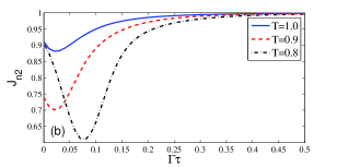
Figure 7: (Color online) The linear correlation coefficients $J_{n2}$ as a function of (a) the transmission rate $T$ ; (b) the collisional dephasing rate $\Gamma\tau$, where $g=2$, $|\alpha|=10$, and $\theta_{2}-\theta_{1}=\pi$, and $\phi=0.062$.

This decorrelation point ($\phi=0$) $J_{x2}(\hat{x}_{a2},\hat{x}_{b2})=0$ is very important for atom-light hybrid interferometer using the homodyne detection Ma . At this point ($\phi=0$) the noise of output field $[\langle(\Delta\hat{x}_{a2})^{2}\rangle=1/4]$ is the same as that of input field and it is the lowest in our scheme as shown in Fig. 2. The optimal phase sensitivity $\Delta\phi_{\text{HD}}$ and the maximal SNR${}_{\text{HD}}$ are obtained at this point with different $\theta_{\alpha}$. The LCC $J_{x2}$ as a function of the transmission rate $T$ and the collisional dephasing rates $\Gamma\tau$ are shown in Fig. 6. With the decrease of the transmission rate $T$ or the increase of $\Gamma\tau$, the LCCs $J_{x2}$ is reduced and tend to $-1$. Due to large loss ($T$ small) or large decoherence ($\Gamma\tau$ large) one arm inside the interferomter (the optical field $\hat{a}_{1}^{\prime}$ or the atomic excitation $\hat{b}_{1}^{\prime}$) is vanished, the decorrelation condition does not exist. Therefore, the serious break of decorrelation condition will degrade the sensitivity in the phase precision measurement.

This decorrelation point ($\phi=0$) $J_{n2}(\hat{n}_{a2},\hat{n}_{b2})=0$ is also very important for the intensity detection. The low noise is dominant in realizing the optimal sensitivity and the maximal SNR. At this point ($\phi=0$), we can obtain the maximal SNR${}_{\text{ID}}$. However, the slope $\left|\partial\langle\hat{n}_{a2}\rangle/\partial\phi\right|$ is equal to $0$ at this decorrelation point as shown in Fig. 3(a). In Fig. 3(b) at nearby the decorrelation point, the noise is amplifed a little and the optimal phase sensitivity $\Delta\phi_{\text{ID}}$ is obtained. With the decrease of the transmission rate $T$ or the increase of $\Gamma\tau$, the LCC $J_{n2}$ are reduced at first, then revive quickly, and finally increase to $1$ as shown in Fig. 7. The behaviors of the two detection methods are different, but both of their correlations eventually tend to strong correlation due to the losses. Therefore, the serious break of decorrelation condition will degrade the sensitivity in the phase precision measurement.

V Conclusions

We gave out the phase sensitivities and the SNRs of the atom-light hybrid interferometer with the method of homodyne detection and intensity detection. Using the homodyne detection, for given input intensity $N_{\alpha}$ and coupling intensity $g$ the optimal sensitivity $\Delta\phi_{\text{HD}}$ and the maximal SNR${}_{\text{HD}}$ is not only dependent on the phase shift $\phi$ but also dependent on the phase $\theta_{\alpha}$ of the input coherent state. We obtain that the sensitivity is low (i.e. $\Delta\phi_{\text{HD}}$ large) when the SNR${}_{\text{HD}}$ is high and vice versa because the optimal point changes with $\theta_{\alpha}$. Using the intensity detection, the optimal sensitivity $\Delta\phi_{\text{ID}}$ and the maximal SNR${}_{\text{ID}}$ is only dependent on the phase shift $\phi$ for given input intensity $N_{\alpha}$ and coupling intensity $g$. Under the balanced condition, the maximal SNR${}_{\text{ID}}$ is obtained when the phase is $0$ and the optimal phase sensitivity $\Delta\phi_{\text{ID}}$ is obtained when the phase is nearby $0$. The loss of light field and atomic decoherence will degrade the sensitivity and the SNR of phase measurement, which can be explained from the break of decorrelation conditions.

VI Acknowledgements

This work was supported by the National Natural Science Foundation of China under Grant Nos. 11474095,  11274118,  11234003, 91536114 and 11129402, and is supported by the Innovation Program of the Shanghai Municipal Education Commission (Grant No. 13ZZ036) and the Fundamental Research Funds for the Central Universities.

References

- (1) C. W. Helstrom, Quantum Detection and Estimation Theory. New York: Academic (1976).
- (2) A. S. Holevo, Probabilistic and Statistical Aspect of Quantum Theory. Amsterdam: North-Holland (1982).
- (3) C. M. Caves, Quantum-mechanical noise in an interferometer, Phys. Rev. D 23, 1693 (1981).
- (4) S. L. Braunstein and C. M. Caves, Statistical Distance and the Geometry of Quantum States, Phys. Rev. Lett. 72, 3439 (1994).
- (5) S. L. Braunstein and C. M. Caves, and G. J. Milburn, Generalized Uncertainty Relations: Theory, Examples, and Lorentz Invariance, Ann. Phys. 247 135 (1996).
- (6) H. Lee, P. Kok, J. P. Dowling, A Quantum Rosetta Stone for Interferometry, J Mod Opt 49 2325 (2002).
- (7) V. Giovannetti, S. Lloyd, and L. Maccone, Quantum Metrology, Phys. Rev. Lett. 96, 010401 (2006).
- (8) M. Zwierz, C. A. Pérez-Delgado, and P. Kok, General Optimality of the Heisenberg Limit for Quantum Metrology, Phys. Rev. Lett. 105, 180402 (2010).
- (9) V. Giovannetti, S. Lloyd, L. Maccone, Quantum-enhanced measurements: beating the standard quantum limit, Science 306, 1330 (2004);
- (10) V. Giovannetti, S. Lloyd, L. Maccone, Advances in quantum metrology, Nature photonics 5, 222 (2011).
- (11) Z. Y. Ou, Enhancement of the phase-measurement sensitivity beyond the standard quantum limit by a nonlinear interferometer, Phys. Rev. A 85, 023815 (2012).
- (12) B. P. Abbott et al., Observation of Gravitational Waves from a Binary Black Hole Merger, Phys. Rev. Lett. 116, 061102 (2016).
- (13) M. Xiao, L. A. Wu, and H. J. Kimble, Precision Measurement beyond the Short Noise Limit, Phys. Rev. Lett. 59, 278 (1987).
- (14) P. Grangier, R. E. Slusher, B. Yurke, and A. LaPorta, Squeezed-Light-Enhanced Polarization Interferometer, Phys. Rev. Lett. 59, 2153 (1987).
- (15) G. Toth and I. Apellaniz, Quantum metrology from a quantum information science perspective, J. Phys. A 47, 424006 (2014).
- (16) L. Pezzè and A. Smerzi, in Proceedings of the International School of Physics “Enrico Fermi”, Course CLXXXVIII “Atom Interferometry” edited by G. Tino and M. Kasevich (Società Italiana di Fisica and IOS Press, Bologna, 2014), p. 691.
- (17) R. Demkowicz-Dobrzanski, M. Jarzyna, J. Kolodynski, Quantum limits in optical interferometry, Progress in Optics 60, 345 (2015).
- (18) J. P. Dowling, Quantum optical metrology–the lowdown on high-N00N states, Contemporary Physics 49, 125 (2008)
- (19) A. N. Boto, P. Kok, D. S. Abrams,S. L. Braunstein, C. P. Williams, and J. P. Dowling, Quantum Interferometric Optical Lithography: Exploiting Entanglement to Beat the Diffraction Limit, Phys. Rev. Lett. 85, 2733 (2000).
- (20) R. Demkowicz-Dobrzanski, U. Dorner, B. J. Smith, J. S. Lundeen, W. Wasilewski, K. Banaszek, and I. A. Walmsley, Quantum phase estimation with lossy interferometers, Phys. Rev. A 80, 013825 (2009).
- (21) B. M. Escher, R. L. de Matos Filho and L. Davidovich, General framework for estimating the ultimate precision limit in noisy quantum-enhanced metrology, Nat. Phys. 7, 406 (2011).
- (22) R. Demkowicz-Dobrzanski, J. Kolodynski, and M. Guta, The elusive Heisenberg limit in quantum-enhanced metrology, Nat. Commun. 3, 1063 (2012).
- (23) D. W. Berry, Michael J. W. Hall, and Howard M. Wiseman, Stochastic Heisenberg Limit: Optimal Estimation of a Fluctuating Phase, Phys. Rev. Lett. 111, 113601 (2013).
- (24) R. Chaves, J. B. Brask, M. Markiewicz, J. Kołodynski, and A. Acin, Noisy Metrology beyond the Standard Quantum Limit, Phys. Rev. Lett. 111, 120401 (2013).
- (25) W. Dur, M. Skotiniotis, F. Frowis, and B. Kraus, Improved Quantum Metrology Using Quantum Error Correction, Phys. Rev. Lett. 112, 080801 (2014).
- (26) E. M. Kessler, I. Lovchinsky, A. O. Sushkov, and M. D. Lukin, Quantum Error Correction for Metrology, Phys. Rev. Lett. 112, 150802 (2014).
- (27) S. Alipour, M. Mehboudi, and A. T. Rezakhani, Quantum Metrology in Open Systems: Dissipative Cramer-Rao Bound, Phys. Rev. Lett. 112, 120405 (2014).
- (28) B. Yurke, S. L. McCall, and J. R. Klauder, SU(2) and SU(1 1) interferometers, Phys. Rev. A 33, 4033 (1986).
- (29) U. Leonhardt, Quantum statistics of a two-mode SU(1,1) interferometer, Phys. Rev. A 49, 1231 (1994).
- (30) A. Vourdas, SU(2) and SU(1,1) phase states, Phys. Rev. A 41, 1653 (1990).
- (31) B. C. Sanders, G. J. Milburn and Z. Zhang, Optimal quantum measurements for phase-shift estim ation in optical interferometry, J. Mod. Optics 44, 1309 (1997).
- (32) W. N. Plick, J. P. Dowling and G. S. Agarwal, Coherent-light-boosted sub-shot noise quantum interferometry, New J. Phys. 12, 083014 (2010).
- (33) J. T. Jing, C. J. Liu, Z. F. Zhou, Z. Y. Ou, and W. P. Zhang, Realization of a Nonlinear Interferometer with Parametric Amplifiers, Appl. Phys. Lett. 99, 011110 (2011).
- (34) T. S. Horrom, B. E. Anderson, P. Gupta, and P. Lett, SU(1,1) interferometry via four-wave mixing in Rb. The 45th Winter Colloquium on the Physics of Quantum Electronics (PQE), 2015.
- (35) A. M. Marino, N. V. Corzo Trejo and P. D. Lett, Effect of losses on the performance of an SU(1,1) interferometer, Phys. Rev. A 86, 023844 (2012).
- (36) F. Hudelist, J. Kong, C. J. Liu, J. Jing, Z. Y. Ou, and W. Zhang, Quantum metrology with parametric amplifier based photon correlation interferometers, Nat. Commun. 5, 3049 (2014).
- (37) C. Gross, T. Zibold, E. Nicklas, J. Est‘eve, andM. K. Oberthaler, Nonlinear atom interferometer surpasses classical precision limit, Nature (London) 464, 1165 (2010).
- (38) Daniel Linnemann, Realization of an SU(1,1) Interferometer with Spinor Bose-Einstein Condensates, Master thesis, University of Heidelberg, 2013.
- (39) J. Peise, B. Lücke, L. Pezzé, F. Deuretzbacher, W. Ertmer, J. Arlt, A. Smerzi, L. Santos and C. Klempt, Interaction-free measurements by quantum Zeno stabilization of ultracold atoms, Nat. Commun. 6, 6811 (2015).
- (40) M. Gabbrielli, L. Pezzé, and A. Smerzi, Spin-mixing interferometry with Bose-Einstein condensates, Phys. Rev. Lett. 115, 163002 (2015).
- (41) L.-M. Duan, M. D. Lukin, J. I. Cirac, and P. Zoller. Long-distance quantum communication with atomic ensembles and linear optics, Nature 414, 413-418 (2001).
- (42) K. Hammerer, A. S. Sørensen, and E. S. Polzik, Quantum interface between light and atomic ensembles. Rev. Mod. Phys. 82, 1041 (2010)
- (43) L. Li, Y. O. Dudin, and A. Kuzmich, Entanglement between light and an optical atomic excitation, Nature 498, 466 (2013).
- (44) L. Q. Chen, G. W. Zhang, C.-H. Yuan, J. Jing, Z. Y. Ou, and W. Zhang, Enhanced Raman scattering by spatially distributed atomic coherence, Appl. Phys. Lett. 95, 041115 (2009).
- (45) L. Q. Chen, G. W. Zhang, C.-L. Bian, C.-H. Yuan, Z. Y. Ou, and W. Zhang, Observation of the Rabi Oscillation of Light Driven by an Atomic Spin Wave, Phys. Rev. Lett. 105, 133603 (2010).
- (46) C.-H. Yuan, L. Q. Chen, J. T. Jing, Z. Y. Ou, and W. Zhang, Coherently enhanced Raman scattering in atomic vapor, Phys. Rev. A 82, 013817 (2010).
- (47) C.-H. Yuan, L. Q. Chen, Z. Y. Ou, and W. Zhang, Correlation-enhanced phase-sensitive Raman scattering in atomic vapors, Phys. Rev. A 87, 053835 (2013).
- (48) B. Chen, C. Qiu, L. Q. Chen, K. Zhang, J. Guo, C.-H. Yuan, Z. Y. Ou, and W. Zhang, Phase sensitive Raman process with correlated seeds, Appl. Phys. Lett. 106, 111103 (2015).
- (49) B. Chen, C. Qiu, S. Chen, J. Guo, L. Q. Chen, Z. Y. Ou, and W. Zhang, Atom-Light Hybrid Interferometer, Phys. Rev. Lett. 115, 043602 (2015).
- (50) H. Ma, D. Li, C.-H. Yuan, L. Q. Chen, Z. Y. Ou, and W. Zhang, SU(1,1)-type light-atom-correlated interferometer, Phys. Rev. A 92, 023847 (2015).
- (51) M. G. Raymer, Quantum state entanglement and readout of collective atomic-ensemble modes and optical wave packets by stimulated Raman scattering, J. Mod. Opt. 51, 1739 (2004).
- (52) R. Lynch, The quantum phase problem: a critical review, Phys. Rep. 256, 367 (1995).
- (53) T. Kim, O. Pfister, M. J. Holland, J. Noh, and J. L. Hall, Influence of decorrelation on Heisenberg-limited interferometry with quantum correlated photons, Phys. Rev. A 57, 4004 (1998).
- (54) Sh. Barzanjeh, D. P. DiVincenzo, and B. M. Terhal, Dispersive qubit measurement by interferometry with parametric amplifiers, Phys. Rev. B 90, 134515 (2014).
- (55) O. Steuernagel and S. Scheel, Approaching the Heisenberg limit with two-mode squeezed states, J. Opt. B: Quantum Semiclass. Opt. 6, S66 (2004).
- (56) D. Li, C.-H. Yuan, Z. Y. Ou, and W. Zhang, The phase sensitivity of an SU(1,1) interferometer with coherent and squeezed-vacuum light, New J. Phys. 16, 073020 (2014).
- (57) M. O. Scully and M. S. Zubairy, Quantum Optics (Cambridge University Press,. 1997).
- (58) C. C. Gerry and P. L. Knight, Introductory Quantum Optics. (Cambridge University Press, Cambridge, 2005).