On sector magnets or transverse electromagnetic fields in cylindrical coordinates

Abstract

The Laplace’s equations for the scalar and vector potentials describing electric or magnetic fields in cylindrical coordinates with translational invariance along azimuthal coordinate are considered. The series of special functions which, when expanded in power series in radial and vertical coordinates, in lowest order replicate the harmonic homogeneous polynomials of two variables are found. These functions are based on radial harmonics found by Edwin M. McMillan in his more-than-40-years ”forgotten” article, which will be discussed. In addition to McMillan’s harmonics, second family of adjoint radial harmonics is introduced, in order to provide symmetric description between electric and magnetic fields and to describe fields and potentials in terms of same special functions. Formulas to relate any transverse fields specified by the coefficients in the power series expansion in radial or vertical planes in cylindrical coordinates with the set of new functions are provided.

This result is no doubt important for potential theory while also critical for theoretical studies, design and proper modeling of sector dipoles, combined function dipoles and any general sector element for accelerator physics. All results are presented in connection with these problems.

I Introduction

Description of sector combined function magnets, and in general any magnet with translational symmetry along azimuthal coordinate in cylindrical coordinates, is very important issue, and, without any particular reference one can say that every modern accelerator code includes such elements. The main idea, which goes back to original 1968 K. Brown’s paper Brown (1968), based on a solution of Laplace’s equation for scalar potential in cylindrical coordinates using the general power series ansatz. Similar approach but for Laplace’s equation for longitudinal component of vector potential can be found for example in Forest (1998). As one can see the approach is the same in most recent books, e.g. in great details in Wiedemann (2015).

Two major bottlenecks should be noticed. In the first place, if one looking for a solution in a form of a series, these series should be truncated. In our case truncation means that potentials do not satisfy the Laplace’s equation anymore, even if symplectic integrators are used for numerical solution (of course potentials can “satisfy” the Laplace’s equation up to desired order by keeping more and more terms in expansion). But more importantly, the recurrence equation is undetermined. That means in every new order of recurrence one have to assign an arbitrary constant, which will affect all other higher order terms. The uncertainty leads to the fact that there is no one particular choice of basis functions; it make it almost impossible to compare different accelerator codes, since different assumptions might be used for representations of basis functions.

The indeterminacy has simple geometrical illustration. Looking for a field with pure normal dipole component on equilibrium orbit in lowest order, one can come up with almost arbitrary shape of magnet’s north pole if south pole is symmetric with respect to midplane. In the case of dipole, series can be truncated by keeping only dipole component. For higher order multipoles in cylindrical coordinates truncation without violation of Laplace’s equation is not possible.

Working on implementation of these magnets for Synergia, I found particular assumptions which let me to summate series for pure electric and magnetic skew and normal multipoles. Further look for symmetry in description allowed to generate full family of solutions where no truncation is required since all series can be summated. While discussing my results with Sergei Nagaitsev, he brought my attention, as we found later to more-than-40-years forgotten, article by McMillan McMillan (1975) of 1975.

Brining together his and my results I would like to present a new description for multipole expansion in cylindrical coordinates. Any transverse field can be expanded in terms of these functions and related to power series field expansion in horizontal or vertical planes. The new approach do not contradict with previous results but embrace it. An ambiguity in choice of coefficients and problem of truncation are resolved. Thus it can be employed for theoretical studies, design and simulation of sector magnets.

I.1 Article structure

Section II describes general equations of motion for a particle in curvilinear coordinates associated with Frenet-Serret frame. The case of transverse electromagnetic fields described in section III.

Subsections III.1,III.2 provide most general equations of motion for pure electric and magnetic fields. Two further subsections III.4,III.5 describes the expansion of fields in multipoles for cases with zero and constant curvatures. The section III.6 relates new family of functions to recurrence equations.

II General equations of motion

II.1 Global coordinates in Lab frame

The Lagrangian of a relativistic particle of mass $m$ with an electric charge $e$ in most general static electromagnetic field is given by

$$\mathcal{L}[\mathbf{R},\dot{\mathbf{R}};t]=-\frac{m\,c^{2}}{\gamma(\mathbf{V})}-e\,\Phi(\mathbf{R})+e\left(\mathbf{V}\cdot\mathbf{A}(\mathbf{R})\right),$$

where $\mathbf{R}=(Q_{1},Q_{2},Q_{3})$ is a position vector in the configuration space of generalized coordinates spanned on three dimensional right-handed Cartesian coordinate system $\{\hat{\mathbf{E}}_{1},\hat{\mathbf{E}}_{2},\hat{\mathbf{E}}_{3}\}$ associated with Lab frame at the facility of a particle accelerator, $\mathbf{V}\equiv\dot{\mathbf{R}}$ is a vector of matching generalized velocities where $\dot{(\ldots)}\equiv\frac{\mathrm{d}}{\mathrm{d}t}$ is the time derivative operator. $\Phi(\mathbf{R})$ and $\mathbf{A}(\mathbf{R})$ are the electric scalar and magnetic vector potentials respectively, and,

$$\gamma(\mathbf{V})=\frac{1}{\sqrt{1-\beta(\mathbf{V})^{2}}}$$

is the relativistic Lorentz factor where $\beta$ is the ratio of $V$ to the speed of light in vacuum, $c$.

Substituting the Lagrangian into the Euler-Lagrange equations (Lagrange’s equations of the second kind)

$$\frac{\mathrm{d}}{\mathrm{d}t}\frac{\partial\,\mathcal{L}}{\partial\dot{\mathbf{R}}}-\frac{\partial\,\mathcal{L}}{\partial\mathbf{R}}=0$$

with shorthand notation

$$\frac{\partial}{\partial\mathbf{a}}=\left(\frac{\partial}{\partial a_{1}},\frac{\partial}{\partial a_{2}},\frac{\partial}{\partial a_{3}}\right)$$

representing a vector of partial derivatives with respect to the indicated variables, gives the equation of motion which is the relativistic form of the Lorentz force

$$\mathbf{F}=e\left[\mathbf{E}+(\mathbf{V}\times\mathbf{B})\right]$$

or explicitly

$$\frac{\mathrm{d}}{\mathrm{d}t}(\gamma\,m\,\dot{Q}_{i})=e\,(E_{i}+\epsilon_{ijk}\dot{Q}_{j}B_{k})$$

where the electric and magnetic fields related to scalar electric and vector magnetic potentials through the gradient and curl vector operators respectively

$$\mathbf{E} = (E_{1},E_{2},E_{3})\equiv\,\,-\,\nabla\,\Phi,$$

$$\mathbf{B} = (B_{1},B_{2},B_{3})\equiv\nabla\times\mathbf{A}.$$

A more abstract formulation can be given in terms of Hamiltonian which describes phase space of canonical variables $\{\mathbf{P},\mathbf{Q}\}$, where $\mathbf{P}$ is the particle’s canonical (total) momentum defined as

$$\mathbf{P}\equiv\frac{\partial\,\mathcal{L}}{\partial\dot{\mathbf{R}}}=\boldsymbol{\Pi}+e\,\mathbf{A}$$

and $\boldsymbol{\Pi}=\gamma\,m\,\mathbf{V}$ being the particle’s kinetic momentum. The Hamiltonian might be constructed using the Legendre transformation of $\mathcal{L}$

$$\mathcal{H}[\mathbf{P},\mathbf{Q};t] = \mathbf{V}\,\mathbf{P}-\mathcal{L}=\sum_{i=1}^{3}\dot{Q}_{i}P_{i}-\mathcal{L}$$

$$= c\,\sqrt{m^{2}c^{2}+\left(\mathbf{P}-e\,\mathbf{A}\right)^{2}}+e\,\Phi.$$

The time evolution of the system is given by Hamilton’s equations

$$\frac{\mathrm{d}\,\mathbf{P}}{\mathrm{d}t}=-\frac{\partial\,\mathcal{H}}{\partial\mathbf{Q}}\qquad\text{and}\qquad\frac{\mathrm{d}\,\mathbf{Q}}{\mathrm{d}t}=\frac{\partial\,\mathcal{H}}{\partial\mathbf{P}}$$

or equivalently

$$\dot{\mathbf{Q}} = c\,\frac{\mathbf{P}-e\,\mathbf{A}}{\sqrt{m^{2}c^{2}+(\mathbf{P}-e\,\mathbf{A})^{2}}},$$

$$\dot{\mathbf{P}} = e\,\left(\nabla\mathbf{A}\right)\cdot\dot{\mathbf{Q}}-e\,\nabla\Phi.$$

The model of accelerator assumes the specification of a reference orbit designed for a particle with certain equilibrium energy and assignment of beam line elements placed along it. In the case of a circular accelerator the closed orbit of a machine with alignment errors in general will not coincide with reference orbit. For most accelerator needs (except e.g. helical orbits for muon cooling) the designed orbit is piecewise flat function, which means that it consists of a series of curves with zero torsion; moreover, usually, these curves are straight lines and circular arcs. In order to better exploit the geometry of beam motion and symmetry of electromagnetic fields we will introduce the local Frenet-Serret frame attached to equilibrium orbit and new global coordinates associated with it (see FIG. 1).

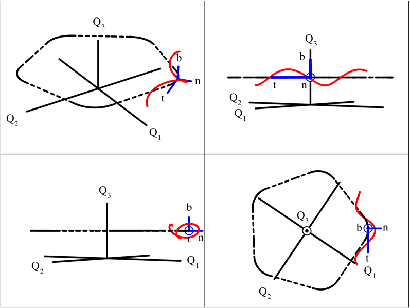
Figure 1: Schematic plot of an equilibrium orbit for an accelerator consisting of five drift spaces and five $72^{\circ}$ bending magnets. Lab frame and local Frenet-Serret frames are shown in black and blue colors respectively. The test particle winding the equilibrium orbit shown in red.

II.2 Global coordinates associated with
Frenet-Serret frame

The equilibrium particle is a particle with design energy perfectly following the reference orbit. Let $\mathbf{R}_{0}(t)$ be the position vector of it as a function of time. Then one can describe the equilibrium orbit in terms of its natural parametrization by arc length as

$$s(t)=\int_{0}^{t}|\dot{\mathbf{R}}_{0}(t)|\,\mathrm{d}\,t.$$

Now on can introduce the local right-handed orthonormal Frenet-Serret basis $\{\hat{\mathbf{n}},\hat{\mathbf{b}},\hat{\mathbf{t}}\}$ (or TNB frame), where basis vectors are defined as follows:

• tangent unit vector

  $$\hat{\mathbf{t}}=\frac{\mathrm{d}\,\mathbf{R}_{0}(s)}{\mathrm{d}s},$$

• outward-pointing normal unit vector

  $$\hat{\mathbf{n}}=-\frac{1}{\kappa(s)}\frac{\mathrm{d}\,\hat{\mathbf{t}}}{\mathrm{d}s},$$

• and binormal unit vector

  $$\hat{\mathbf{b}}=\hat{\mathbf{t}}\times\hat{\mathbf{n}},$$

where $\kappa=\left|\mathrm{d}\,\hat{\mathbf{t}}/\mathrm{d}s\right|$ defines the local curvature of the equilibrium orbit. Then, using the Frenet-Serret formulas describing the derivatives of unit vectors in terms of each other

$$\mathrm{d}\begin{bmatrix}\hat{\mathbf{t}}\\ \hat{\mathbf{n}}\\ \hat{\mathbf{b}}\end{bmatrix}=\begin{bmatrix}0&-\kappa&0\\ \kappa&0&\tau\\ 0&-\tau&0\end{bmatrix}\begin{bmatrix}\hat{\mathbf{t}}\\ \hat{\mathbf{n}}\\ \hat{\mathbf{b}}\end{bmatrix}\mathrm{d}s$$

where $\tau(s)$ is the torsion of an equilibrium orbit which measures the failure of a curve to be planar, one can express the position vector of a test particle as a transverse displacement from equilibrium orbit, see FIG. 2,

$$\mathbf{R}(s)=\mathbf{R}_{0}(s)+\mathbf{r}(s)=\mathbf{R}_{0}(s)+q_{1}\hat{\mathbf{n}}+q_{2}\hat{\mathbf{b}}.$$

and its’ infinitesimally small displacement

$$\mathrm{d}\mathbf{R}=\hat{\mathbf{n}}\,\mathrm{d}q_{1}+\hat{\mathbf{b}}\,\mathrm{d}q_{2}+(1+\kappa\,q_{1})\hat{\mathbf{t}}\,\mathrm{d}q_{3}+\tau(q_{1}\hat{\mathbf{b}}-q_{2}\hat{\mathbf{n}})\mathrm{d}q_{3},$$

where $(q_{1},q_{2},q_{3})$ are local curvilinear coordinates spanned on $(\hat{\mathbf{n}},\hat{\mathbf{b}},\hat{\mathbf{t}})$. One can see that in the case of flat orbit, i.e. $\tau=0$, the local Frenet-Serret frame can be associated with global orthogonal coordinate system with a line element in a form

$$\mathrm{d}\mathbf{l}=\sum_{i=1}^{3}h_{i}\hat{\mathbf{e}}_{i}\mathrm{d}q_{i},$$

where scale factors are $h_{1}=h_{2}=1$ and $h\equiv h_{3}=1+\kappa\,q_{1}$.

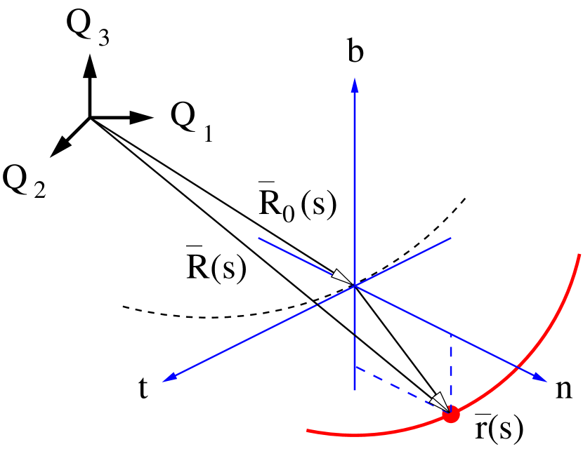
Figure 2: Illustration of a test particle’s position vector expressed as a transverse, i.e. for fixed $q_{3}$, displacement from equilibrium orbit.

The use of global coordinates with metric provided by local Frenet-Serret frame allows to rewrite the Lagrangian as

$$\mathcal{L}[\mathbf{r},\dot{\mathbf{r}};t]=-m\,c^{2}\sqrt{1-\frac{v^{2}}{c^{2}}}-e\,\Phi+e\,\mathbf{v}\cdot\mathbf{A},$$

where $\mathbf{v}=(\dot{q}_{1},\dot{q}_{2},h\,\dot{q}_{3})$ is the particle’s velocity expressed in new coordinates. Thus the new equations of motion are

$$\frac{\mathrm{d}}{\mathrm{d}t}(\gamma\,m\,\mathbf{v})=e\left(\mathbf{E}+\epsilon_{ijk}\,\hat{\mathbf{e}}_{i}\,v_{j}\,B_{k}\right)+\gamma\,m\,\dot{q}_{3}^{2}\,\mathbf{K}$$

where the vector in the RHS of equation defined as

$$\mathbf{K}=(\kappa\,h,0,\kappa^{\prime}\,q_{1}),$$

and the operator $(\ldots)^{\prime}\equiv\frac{\mathrm{d}}{\mathrm{d}q_{3}}$ is the derivative with respect to longitudinal coordinate. Derivatives of potentials expressed via electromagnetic fields using expressions for differential operators in curvilinear orthogonal coordinates form Table 1. Calculating components of the new canonical momenta

$$\frac{p_{i}}{h_{i}}\equiv\frac{1}{h_{i}}\frac{\partial\,\mathcal{L}}{\partial\dot{q}_{i}}=\gamma\,m\,v_{i}+e\,\mathbf{A}_{i}(\mathbf{r})$$

allows to write down the new Hamiltonian

$$\mathcal{H}[\mathbf{p},\mathbf{q};t]=c\,\sqrt{m^{2}c^{2}+\sum_{i=1}^{3}\left(\frac{p_{i}-e\,h_{i}A_{i}}{h_{i}}\right)^{2}}+e\,\Phi$$

and equations of motion

$$\dot{q}_{i}\times h_{i} = \frac{c^{2}}{\mathcal{H}-e\,\Phi}\,\frac{p_{i}-e\,h_{i}A_{i}}{h_{i}},$$

$$\dot{p}_{i}\,\,/\,h_{i} = \frac{c^{2}}{\mathcal{H}-e\,\Phi}\left[e\,\epsilon_{ijk}\frac{p_{j}}{h_{j}}\,B_{k}+\frac{K_{i}}{h^{2}}\left(\frac{p_{3}-e\,h\,A_{3}}{h}\right)^{2}\right]$$

$$+e\,E_{i}.$$

Table 1: Differential operators in general orthogonal coordinates $(q_{1},q_{2},q_{3})$ where $H=h_{1}h_{2}h_{3}$, and its expressions in orthogonal coordinates associated with Serret-Frenet frame.

Gradient	$\nabla\phi$	$\displaystyle\sum_{k=1}^{3}\frac{1}{h_{k}}\frac{\partial\,\phi}{\partial q^{k}}\hat{\mathbf{e}}_{k}$
		$\displaystyle\frac{\partial\,\phi}{\partial q_{1}}\,\hat{\mathbf{e}}_{1}+\frac{\partial\,\phi}{\partial q_{2}}\,\hat{\mathbf{e}}_{2}+\frac{1}{h}\frac{\partial\,\phi}{\partial q_{3}}\,\hat{\mathbf{e}}_{3}$
Divergence	$\nabla\cdot\mathbf{F}$	$\displaystyle\sum_{k=1}^{3}\frac{1}{H}\frac{\partial}{\partial q^{k}}\left(\frac{H}{h_{k}}F_{k}\right)$
		$\displaystyle\frac{1}{h}\left[\frac{\partial(h\,F_{1})}{\partial q_{1}}+\frac{\partial(h\,F_{2})}{\partial q_{2}}+\frac{\partial\,F_{3}}{\partial q_{3}}\right]$
Curl	$\nabla\times\mathbf{F}$	$\displaystyle\sum_{k=1}^{3}\frac{h_{k}\,\hat{\mathbf{e}}_{k}}{H}\epsilon_{ijk}\frac{\partial}{\partial q^{i}}\left(h_{j}F_{j}\right)$
		$\displaystyle\frac{1}{h}\left[\frac{\partial(h\,F_{3})}{\partial q_{2}}-\frac{\partial\,F_{2}}{\partial q_{3}}\right]\hat{\mathbf{e}}_{1}+\frac{1}{h}\left[\frac{\partial\,F_{1}}{\partial q_{3}}-\frac{\partial(h\,F_{3})}{\partial q_{1}}\right]\hat{\mathbf{e}}_{2}+\left[\frac{\partial\,F_{2}}{\partial q_{1}}-\frac{\partial\,F_{1}}{\partial q_{2}}\right]\hat{\mathbf{e}}_{3}$
Scalar Laplacian	$\triangle\phi=\nabla\cdot(\nabla\phi)$	$\displaystyle\sum_{k=1}^{3}\frac{1}{H}\frac{\partial}{\partial q^{k}}\left(\frac{H}{h_{k}^{2}}\frac{\partial\,\phi}{\partial q^{k}}\right)$
		$\displaystyle\frac{1}{h}\left[\frac{\partial}{\partial q_{1}}\left(h\frac{\partial\,\phi}{\partial q_{1}}\right)+\frac{\partial}{\partial q_{2}}\left(h\frac{\partial\,\phi}{\partial q_{2}}\right)+\frac{\partial}{\partial q_{3}}\left(\frac{1}{h}\frac{\partial\,\phi}{\partial q_{3}}\right)\right]$
Vector Laplacian	$\davidsstar\mathbf{F}=\nabla(\nabla\cdot\mathbf{F})-\nabla\times(\nabla\times\mathbf{F})$	$\displaystyle\sum_{k=1}^{3}\left\{\frac{1}{h_{k}}\frac{\partial}{\partial q^{k}}\left[\frac{1}{H}\frac{\partial}{\partial q^{i}}\left(\frac{H}{h_{i}}F_{i}\right)\right]-\frac{h_{k}}{H}\epsilon_{ijk}\frac{\partial}{\partial q^{i}}\left[\frac{h_{j}^{2}\hat{\mathbf{e}}_{j}}{H}\epsilon_{lmj}\frac{\partial}{\partial q^{l}}(h_{m}F_{m})\right]\right\}\hat{\mathbf{e}}_{k}$

III Transverse electromagnetic fields

Now we will restrict ourself with the case of transverse electromagnetic fields; in orthogonal curvilinear coordinate system associated with Serret-Frenet frame these are the fields with translation symmetry along longitudinal coordinate $q_{3}$. Thus, the scalar and vector potentials are function of transverse coordinates only and vector potential has only one nonvanishing component which is $A_{3}$. Both potentials satisfies Laplace equation

$$\triangle\Phi = \frac{1}{h}\left[\frac{\partial}{\partial q_{1}}\left(h\frac{\partial\,\Phi}{\partial q_{1}}\right)+\frac{\partial}{\partial q_{2}}\left(h\frac{\partial\,\Phi}{\partial q_{2}}\right)\right]=0,$$

$$\davidsstar\mathbf{A} = \frac{\partial}{\partial q_{1}}\left[\frac{1}{h}\frac{\partial\,(h\,A_{3})}{\partial q_{1}}\right]+\frac{\partial}{\partial q_{2}}\left[\frac{1}{h}\frac{\partial\,(h\,A_{3})}{\partial q_{2}}\right]=0.$$

The corresponding fields are given by Maxwell equations

$$\mathbf{E}=-\nabla\Phi\qquad\text{and}\qquad\mathbf{B}=\nabla\times\mathbf{A}$$

with differential operators defined for orthogonal curvilinear coordinate system (Table 1), and one gets

$$E_{1} = -\frac{\partial\,\Phi}{\partial q_{1}},\qquad\qquad B_{1}=\,\,\,\,\frac{1}{h}\frac{\partial(h\,A_{3})}{\partial q_{2}},$$

$$E_{2} = -\frac{\partial\,\Phi}{\partial q_{2}},\qquad\qquad B_{2}=-\frac{1}{h}\frac{\partial(h\,A_{3})}{\partial q_{1}}.$$

III.1 $t$-representation

In the case of pure electric or magnetic fields further simplifications can be applied. For numerical integration purposes it is very convenient to have a Hamiltonian in a form of a sum of “kinetic” and “potential” energies where potentials will be separated from momentum variables. In this case, one can easily construct symplectic integrator consisting of “drifts” and “kicks” associated with kinetic and potential terms respectively (e.g. Yoshida (1990)).

For pure electric field when curvature is independent of longitudinal coordinate not only Hamiltonian but also $p_{3}$ is an invariant of motion, and, problem is essentially two dimensional. Measuring the time in units of $c\,t$ and normalizing the transverse momentums over the longitudinal component, $\tilde{p}_{1,2}=p_{1,2}/p_{3}$, one has

$$\mathrm{H}[\tilde{\mathbf{p}},\mathbf{q};c\,t]=\frac{1}{h}\sqrt{\frac{p_{3}^{2}+h^{2}m^{2}c^{2}}{p_{3}^{2}}+h^{2}(\tilde{p}_{1}^{2}+\tilde{p}_{2}^{2})}+\frac{e}{p_{3}\,c}\,\Phi.$$

We will call this model Hamiltonian the $t$-representation; with no assumptions made, but the field symmetry, we derived general equations of motion which can be used for the basis for the construction of symplectic integrator. In a paraxial approximation, $\tilde{p}_{1,2}\ll 1$,and for $p_{1,2}\gg m\,c$ the form is significantly simpler, and a limit of straight coordinates when $h=1$ is obvious

$$\mathrm{H}[\tilde{\mathbf{p}},\mathbf{q};c\,t]\approx h\,\left(\frac{\tilde{p}_{1}^{2}}{2}+\frac{\tilde{p}_{2}^{2}}{2}\right)+\frac{1}{h}+\frac{e}{p_{3}\,c}\,\Phi.$$

III.2 $s$-representation

For pure magnetic field the Hamiltonian is very hard to exploit since it has only a square root and so no terms to split. Introducing an extended Hamiltonian with a new fictitious time parameter, $\tau$, where the old independent variable and old Hamiltonian with a negative sign will be treated as an additional pair of canonically conjugated coordinates, $(-\mathcal{H},t)$, one have:

$$0 \equiv \mathcal{O}[p_{1},p_{2},p_{3},-\mathcal{H};q_{1},q_{2},q_{3},t;\tau]$$

$$= c\,\sqrt{m^{2}c^{2}+p_{1}^{2}+p_{2}^{2}+\left(\frac{p_{3}-e\,h\,A_{3}}{h}\right)^{2}}-\mathcal{H}.$$

Integration of additional equations of motion gives

$$\mathcal{H}=\mathrm{inv}\qquad\text{and}\qquad t=\tau+C_{0},$$

where we can set a constant of integration $C_{0}=0$.

If curvature is invariant of longitudinal coordinate the longitudinal component of momentum conserved, as well as in the case of electric field, and we will use $-p_{3}$ as a new Hamiltonian, reducing number of degrees of freedom back up to three by using $q_{3}$ as a new independent variable:

$$-p_{3} \equiv \mathcal{K}[p_{1},p_{2},-\mathcal{H};q_{1},q_{2},t;q_{3}]$$

$$= -h\,\sqrt{\left(\frac{\mathcal{H}}{c}\right)^{2}-m^{2}c^{2}-p_{1}^{2}-p_{2}^{2}}-e\,h\,A_{3}.$$

The use of generating function

$$G_{2}(t,-\Pi)=-t\sqrt{\Pi^{2}c^{2}+(m\,c^{2})^{2}}$$

will allow to use the full kinetic momentum $-\Pi$ of a particle instead of $-\mathcal{H}$ as one of canonical momentums:

$$\mathcal{K}[p_{1},p_{2},-\Pi;q_{1},q_{2},l;q_{3}]=-h\,\sqrt{\Pi^{2}-p_{1}^{2}-p_{2}^{2}}-e\,h\,A_{3},$$

where corresponding canonical coordinate is a particle’s traversed path $l=-\partial\,G_{2}/\partial\Pi=\beta c\,t.$

Since the Hamiltonian do not explicitly depends on $l$, full momentum $\Pi$ is conserved and we can exclude associated degree of freedom using the further renormalization of the Hamiltonian $\mathcal{K}\rightarrow\mathrm{K}\equiv\mathcal{K}/\Pi$, which can be achieved by re-normalizing transverse components of canonical momentums $p_{1,2}\rightarrow\tilde{p}_{1,2}=p_{1,2}/\Pi$:

$$-\frac{p_{3}}{\Pi} \equiv \mathrm{K}[\tilde{p}_{1},\tilde{p}_{2};q_{1},q_{2};q_{3}]$$

$$= -h\,\sqrt{1-\tilde{p}_{1}^{2}-\tilde{p}_{2}^{2}}-\frac{e}{\Pi}\,h\,A_{3}.$$

We will call this model Hamiltonian $s$-representation since the longitudinal coordinate (sometimes referred to the natural parameter along equilibrium orbit, $s$) is used as a time-parameter. This representation is convenient to use for the numerical integrator construction for transverse magnetic fields. The paraxial approximation, $\tilde{p}_{1,2}\ll 1$, gives

$$\mathrm{K}[\tilde{\mathbf{p}},\mathbf{q};q_{3}]\approx h\,\left(\frac{\tilde{p}_{1}^{2}}{2}+\frac{\tilde{p}_{2}^{2}}{2}\right)-h-\frac{e}{\Pi}\,h\,A_{3}.$$

III.3 R- and S-elements

So far we provided dynamical equations of motion without specifying how to represent electromagnetic fields. In next two subsections we will discuss the multipole field expansion for two most important types of elements: R-element for $\kappa=0$ and S-element defined for $\kappa=\text{const}=1/R_{0}$.

R- stays for rectangular and this element is the one whit $(q_{1},q_{2},q_{3})$ simply being the right handed Cartesian coordinate system which we will denote as $(x,y,z)$. All fields in such an element are invariant along $z$ axis and usually serves the function of regular quadrupoles, sextupoles, octupoles or combined function correctors. In addition one can design pure R-dipoles, while combined function bending magnets are exotic and very complicated since equilibrium orbit will not anymore coincides with axis of symmetry.

S-element is the element defined whit natural sector coordinate system. Defining the set of normalized coordinates $(x=q_{1}/R_{0},y=q_{2}/R_{0},z=q_{3}/R_{0})$, one can see that it simply can be related to normalized right handed cylindrical coordinates $(\rho=1+x,y,\theta=z/R_{0})$, see FIG. 3, and thus all fields are invariant along azimuthal coordinate $\theta$. S-elements are suitable for the design of combined function bending magnets, since in contrast to R-elements, equilibrium orbit follows along $\theta$.

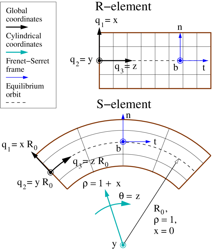
Figure 3: Illustration of R- and S- elements. Elements are shown in brown. Global curvilinear coordinates with associated grid lines are shown in black. Black dashed line represent an equilibrium orbit. An example of Frenet-Serret frame attached to an equilibrium orbit drawn in blue colors. For S-element, an additional right-handed normalized cylindrical system is added and shown in cyan.

Table 2: Harmonic homogeneous polynomials in two variables.

$n$	$\mathcal{A}_{n}$	$\mathcal{B}_{n}$
0	1	0
1	$x$	$y$
2	$x^{2}-y^{2}$	$2\,x\,y$
3	$x^{3}-3\,x\,y^{2}$	$3\,x^{2}y-y^{3}$
4	$x^{4}-6\,x^{2}y^{2}+y^{4}$	$4\,x^{3}y-4\,x\,y^{3}$
5	$x^{5}-10\,x^{3}y^{2}+5\,x\,y^{4}$	$5\,x^{4}y-10\,x^{2}y^{3}+y^{5}$
6	$x^{6}-15\,x^{4}y^{2}+15\,x^{2}y^{4}-y^{6}$	$6\,x^{5}y-20\,x^{3}y^{3}+6\,x\,y^{5}$
7	$x^{7}-21\,x^{5}y^{2}+35\,x^{3}y^{4}-7\,x\,y^{6}$	$7\,x^{6}y-35\,x^{4}y^{3}+21\,x^{2}y^{5}-y^{7}$
8	$x^{8}-28\,x^{6}y^{2}+70\,x^{5}y^{4}-84\,x^{3}y^{6}+9\,x\,y^{8}$	$8\,x^{7}y-56\,x^{5}y^{3}+56\,x^{3}y^{5}-8\,x\,y^{7}$
9	$x^{9}-36\,x^{7}y^{2}+126\,x^{5}y^{4}-84\,x^{3}y^{6}+9\,x\,y^{8}$	$9\,x^{8}y-84\,x^{6}y^{3}+126\,x^{4}y^{5}-36\,x^{2}y^{7}+y^{9}$

III.4 Multipoles in Cartesian coordinates

In Cartesian coordinates Laplace equations for electro- and magnetostatic fields are in the same form which significantly simplify the problem

$$\triangle_{\perp}\Phi = \frac{\partial^{2}\Phi}{\partial x^{2}}+\frac{\partial^{2}\Phi}{\partial y^{2}}=0,$$

$$\davidsstar_{\perp}\mathbf{A} = \left(\frac{\partial^{2}A_{z}}{\partial x^{2}}+\frac{\partial^{2}A_{z}}{\partial y^{2}}\right)\hat{\mathbf{e}}_{z}=0.$$

Introduction of complex variables allows a very compact description of a problem with unified description of electric and magnetic fields. Suppose we have a holomorphic function of complex variable $\mathcal{Z}=x+i\,y$ which we will call complex scalar potential which real part is defined to be a longitudinal component of a vector potential and imaginary part is the electric scalar potential

$$\Omega(\mathcal{Z})=A_{z}(x,y)+i\,\Phi(x,y).$$

Since real or imaginary part of any holomorphic function are harmonic functions, $A_{z}$ and $\Phi$ automatically satisfies the Laplace equation. Indeed, suppose we have a vector field $\mathbf{F}=(F_{x},F_{y})$. Introducing the Wirtinger derivatives

$$\frac{\partial}{\partial\mathcal{Z}}=\frac{1}{2}\left(\frac{\partial}{\partial x}-i\,\frac{\partial}{\partial y}\right)\quad\text{and}\quad\frac{\partial}{\partial\overline{\mathcal{Z}}}=\frac{1}{2}\left(\frac{\partial}{\partial x}+i\,\frac{\partial}{\partial y}\right)$$

one can write

$$\frac{\partial\,\Omega}{\partial\overline{\mathcal{Z}}} = 0,$$

$$\frac{\partial\,\Omega}{\partial\mathcal{Z}} = F(\mathcal{Z}),$$

where first equation is the Cauchy-Riemann condition for $\Omega$ which guarantees that this field can be implemented via either magnetic or electric potentials:

$$F_{x} = -\frac{\partial\,\Phi}{\partial x}=\,\,\,\,\frac{\partial\,A_{z}}{\partial y},$$

$$F_{y} = -\frac{\partial\,\Phi}{\partial y}=-\frac{\partial\,A_{z}}{\partial x}.$$

The second equation defines complex function of field components such that

$$F_{x}=-\Im\,F(\mathcal{Z})\quad\text{and}\quad F_{y}=-\Re\,F(\mathcal{Z}),$$

which all together are equivalent to $\mathbf{F}=-\nabla\Phi=\nabla\times\mathbf{A}$. The complex function $F(\mathcal{Z})$ is the holomorphic function again and Cauchy-Riemann equation gives

$$\frac{\partial\,F}{\partial\overline{\mathcal{Z}}}=0,$$

that asserts that field $\mathbf{F}$ is irrotational and divergence free which is equivalent to time-independent free of electric charge and current densities Maxwell’s equations

$$\nabla\cdot\mathbf{F}=0\quad\text{and}\quad\nabla\times\mathbf{F}=0.$$

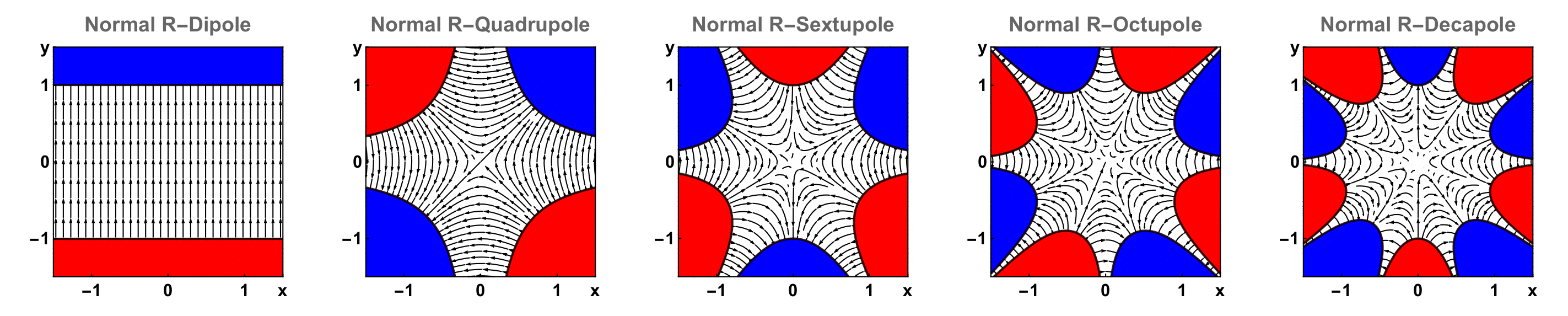
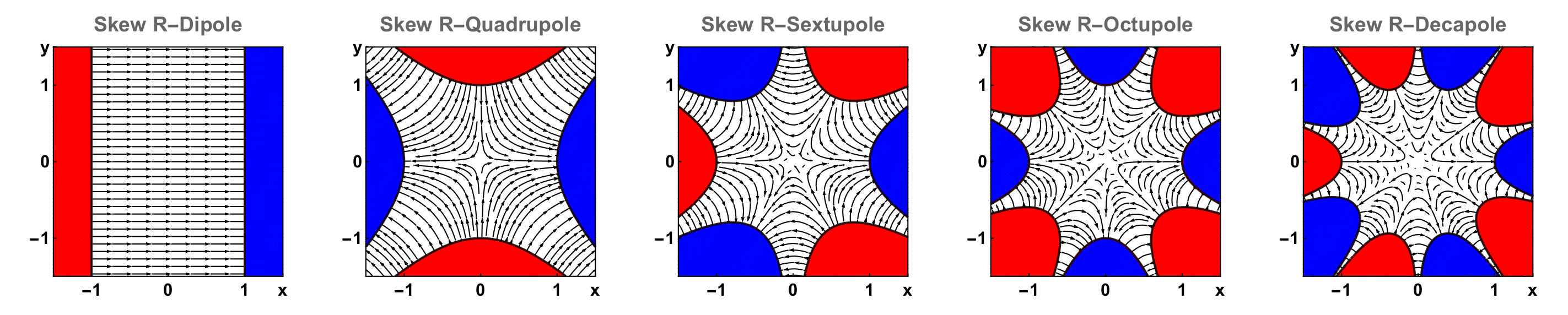
Figure 4: Normal and skew $2n$-pole magnets in Cartesian coordinates. Each figure shows magnetic (electric) field streamlines and poles’ shape in transverse cross section. North (positive electrostatic potential) and south (negative electrostatic potential) poles are shown in red and blue and are given by $(\mathcal{B,A})_{n}=\mp R_{\text{p}}^{n}$ respectively, where $R_{\text{p}}$ is the distance to the pole’s tip.

For accelerator physics purposes the expansion of fields usually represented in terms of homogeneous harmonic polynomials of two variables, which are defined through the complex power function

$$\mathcal{A}_{n}(x,y) = \Re\,\mathcal{Z}^{n}=\frac{1}{2}\left[\left(x+i\,y\right)^{n}+\left(x-i\,y\right)^{n}\right]$$

$$= \sum_{k=0}^{n}\begin{pmatrix}n\\ k\end{pmatrix}x^{n-k}y^{k}\cos\frac{k\,\pi}{2},$$

$$\mathcal{B}_{n}(x,y) = \Im\,\mathcal{Z}^{n}=\frac{1}{2\,i}\left[\left(x+i\,y\right)^{n}-\left(x-i\,y\right)^{n}\right]$$

$$= \sum_{k=0}^{n}\begin{pmatrix}n\\ k\end{pmatrix}x^{n-k}y^{k}\sin\frac{k\,\pi}{2}.$$

Explicit expressions up to 10-th order are in Table 2. These functions satisfy the Laplace equation $\triangle_{\perp}=0$ and related to each other through Cauchy-Riemann equation as

$$\frac{\partial\,\mathcal{A}_{n}}{\partial x}=\frac{\partial\,\mathcal{B}_{n}}{\partial y}\quad\text{and}\quad\frac{\partial\,\mathcal{A}_{n}}{\partial y}=-\frac{\partial\,\mathcal{B}_{n}}{\partial x}.$$

In addition one can introduce “ladder-like” lowering differential operators as

$$n\,\left\{\mathcal{A,B}\right\}_{n-1}=\frac{\partial}{\partial x}\left\{\mathcal{A,B}\right\}_{n}=\pm\frac{\partial}{\partial y}\left\{\mathcal{B,A}\right\}_{n}.$$

Thus one can define two independent of each other sets of solutions, normal (sometimes called upright or straight) and skew pure multipoles, which we will denote with overline $\overline{(\ldots)}$ and underline $\underline{(\ldots)}$ respectively. The complex scalar potentials of pure multipoles are:

$$\overline{\Omega}^{(n)}=-\,\,\overline{C}_{n}\frac{\mathcal{Z}^{n}}{n!}\qquad\text{and}\qquad\underline{\Omega}^{(n)}=-i\,\underline{C}_{\,n}\frac{\mathcal{Z}^{n}}{n!}$$

where $\overline{C}_{n}$ and $\underline{C}_{\,n}$ are coefficients determining the strength of magnets. Corresponding vector fields are defined to have an odd and even midplane symmetries

$$\overline{F}_{\,\text{y}}^{(n)}(x,y) = \overline{F}_{\,\text{y}}^{(n)}(x,-y)\qquad\text{and}\qquad\overline{F}_{\,\text{x}}^{(n)}(x,0)=0,$$

$$\underline{F}_{\,\text{x}}^{(n)}(x,y) = \underline{F}_{\,\text{x}}^{(n)}(x,-y)\qquad\text{and}\qquad\underline{F}_{\,\text{y}}^{(n)}(x,0)=0.$$

Formulas for potentials and fields are listed below in Table 3 and exact expressions are provided in Appendix A. Figure 4 shows the cross section of idealized multipole magnet’s poles and corresponding fields.

Table 3: Formulas for the scalar potential, longitudinal component of the vector potential and field components for pure normal and skew $2n$-poles in Cartesian coordinates.

Normal	Skew
$\displaystyle\overline{\Phi}^{(n)}=-\overline{C}_{n}\frac{\mathcal{B}_{n}}{n!}$	$\displaystyle\underline{\Phi}^{(n)}=-\underline{C}_{\,n}\frac{\mathcal{A}_{n}}{n!}$
$\displaystyle\overline{A}_{z}^{(n)}=-\overline{C}_{n}\frac{\mathcal{A}_{n}}{n!}$	$\displaystyle\underline{A}_{\,z}^{(n)}=\quad\!\!\underline{C}_{\,n}\frac{\mathcal{B}_{n}}{n!}$
$\displaystyle\overline{F}_{\,\text{x}}^{(n)}=\quad\!\!\overline{C}_{n}\frac{\mathcal{B}_{n-1}}{(n-1)!}$	$\displaystyle\underline{F}_{\,\text{x}}^{(n)}=\quad\!\!\underline{C}_{\,n}\frac{\mathcal{A}_{n-1}}{(n-1)!}$
$\displaystyle\overline{F}_{\,\text{y}}^{(n)}=\quad\!\!\overline{C}_{n}\frac{\mathcal{A}_{n-1}}{(n-1)!}$	$\displaystyle\underline{F}_{\,\text{y}}^{(n)}=-\underline{C}_{\,n}\frac{\mathcal{B}_{n-1}}{(n-1)!}$

Therefore, if one provided with experimental data of the power series expansions of the fields in a horizontal or vertical planes

$$\left.F_{x}\right|_{x=0} = \left.F_{x}\right|_{\text{eq}}+\frac{y}{1!}\,\left.\frac{\partial\,F_{x}}{\partial y}\right|_{\text{eq}}+\frac{y^{2}}{2!}\,\left.\frac{\partial^{2}\,F_{x}}{\partial y^{2}}\right|_{\text{eq}}+\ldots,$$

$$\left.F_{y}\right|_{x=0} = \left.F_{y}\right|_{\text{eq}}+\frac{y}{1!}\,\left.\frac{\partial\,F_{y}}{\partial y}\right|_{\text{eq}}+\frac{y^{2}}{2!}\,\left.\frac{\partial^{2}\,F_{y}}{\partial y^{2}}\right|_{\text{eq}}+\ldots,$$

$$\left.F_{x}\right|_{y=0} = \left.F_{x}\right|_{\text{eq}}+\frac{x}{1!}\,\left.\frac{\partial\,F_{x}}{\partial x}\right|_{\text{eq}}+\frac{x^{2}}{2!}\,\left.\frac{\partial^{2}\,F_{x}}{\partial x^{2}}\right|_{\text{eq}}+\ldots,$$

$$\left.F_{y}\right|_{y=0} = \left.F_{y}\right|_{\text{eq}}+\frac{x}{1!}\,\left.\frac{\partial\,F_{y}}{\partial x}\right|_{\text{eq}}+\frac{x^{2}}{2!}\,\left.\frac{\partial^{2}\,F_{y}}{\partial x^{2}}\right|_{\text{eq}}+\ldots,$$

the field derivatives on equilibrium orbit can be related to strength coefficients, see Table 4, which allows to expand a general R-element in terms of pure multipoles.

Table 4: Relationship between coefficients determining the strength of pure R-multipoles and power series expansion of field in horizontal and vertical planes on equilibrium orbit.

	$x=0$		$y=0$
$n$	$\overline{C}_{n}$	$\underline{C}_{\,n}$	$\overline{C}_{n}$	$\underline{C}_{\,n}$
1	$F_{y}$	$F_{x}$	$F_{y}$	$F_{x}$
2	$\partial_{y}\,F_{x}$	$-\partial_{y}\,F_{y}$	$\partial_{x}\,F_{y}$	$\partial_{x}\,F_{x}$
3	$-\partial_{y}^{2}\,F_{y}$	$-\partial_{y}^{2}\,F_{x}$	$\partial_{x}^{2}\,F_{y}$	$\partial_{x}^{2}\,F_{x}$
4	$-\partial_{y}^{3}\,F_{x}$	$\partial_{y}^{3}\,F_{y}$	$\partial_{x}^{3}\,F_{y}$	$\partial_{x}^{3}\,F_{x}$
5	$\partial_{y}^{4}\,F_{y}$	$\partial_{y}^{4}\,F_{x}$	$\partial_{x}^{4}\,F_{y}$	$\partial_{x}^{4}\,F_{x}$

III.5 Multipoles in cylindrical coordinates

In the normalized right-handed cylindrical coordinate system the Laplace equations are

$$\triangle_{\curvearrowright}\Phi = \triangle_{\perp}\Phi+\frac{1}{\rho}\frac{\partial\,\Phi}{\partial\rho}$$

$$= \frac{\partial^{2}\Phi}{\partial\rho^{2}}+\frac{1}{\rho}\frac{\partial\,\Phi}{\partial\rho}+\frac{\partial^{2}\Phi}{\partial y^{2}}=0,$$

$$\davidsstar_{\curvearrowright}\mathbf{A} = \left(\triangle_{\curvearrowright}A_{\theta}-\frac{A_{\theta}}{\rho^{2}}\right)\hat{\mathbf{e}}_{\theta}$$

$$= \left(\frac{\partial^{2}A_{\theta}}{\partial\rho^{2}}+\frac{1}{\rho}\frac{\partial\,A_{\theta}}{\partial\rho}+\frac{\partial^{2}A_{\theta}}{\partial y^{2}}-\frac{A_{\theta}}{\rho^{2}}\right)\hat{\mathbf{e}}_{\theta}=0.$$

Compared to the case with Cartesian coordinates these equations look quite different from each other. In order to retain the symmetry one can note that

$$(\davidsstar_{\curvearrowright}\mathbf{A})_{\theta}=\frac{1}{\rho}\left[\frac{\partial^{2}}{\partial\rho^{2}}-\frac{1}{\rho}\frac{\partial}{\partial\rho}+\frac{\partial^{2}}{\partial y^{2}}\right]\left(\rho\,A_{\theta}\right).$$

Thus looking for the solution in a form similar to harmonic homogeneous polynomials

$$\Phi = -\sum_{k=0}^{n}\phantom{\frac{1}{\rho}}\frac{\mathcal{F}_{n-k}(\rho)}{(n-k)!}\frac{y^{k}}{k!}\left(\overline{C}_{n}\,\sin\frac{k\,\pi}{2}+\underline{C}_{\,n}\,\cos\frac{k\,\pi}{2}\right),$$

$$A_{\theta} = -\sum_{k=0}^{n}\frac{1}{\rho}\frac{\mathcal{G}_{n-k}(\rho)}{(n-k)!}\frac{y^{k}}{k!}\left(\overline{C}_{n}\,\cos\frac{k\,\pi}{2}-\underline{C}_{\,n}\,\sin\frac{k\,\pi}{2}\right),$$

where $\mathcal{F}_{n}(\rho)$ and $\mathcal{G}_{n}(\rho)$ are the functions to be determined, one can find two recurrence equations

$$\frac{\partial^{2}\mathcal{F}_{n}(\rho)}{\partial\rho^{2}}+\frac{1}{\rho}\frac{\partial\,\mathcal{F}_{n}(\rho)}{\partial\rho} = n\,(n-1)\,\mathcal{F}_{n-2}(\rho),$$

$$\frac{\partial^{2}\mathcal{G}_{n}(\rho)}{\partial\rho^{2}}-\frac{1}{\rho}\frac{\partial\,\mathcal{G}_{n}(\rho)}{\partial\rho} = n\,(n-1)\,\mathcal{G}_{n-2}(\rho).$$

They relate $\mathcal{F}_{n}$ and $\mathcal{G}_{n}$ to each other through

$$\mathcal{G}_{n-1}=\frac{1}{n}\,\rho\,\frac{\partial\,\mathcal{F}_{n}}{\partial\rho}\qquad\text{and}\qquad\mathcal{F}_{n-1}=\frac{1}{n}\frac{1}{\rho}\frac{\partial\,\mathcal{G}_{n}}{\partial\rho}.$$

and allows to construct lowering operators

$$\mathcal{F}_{n} = \frac{1}{(n+1)(n+2)}\left[\frac{1}{\rho}\frac{\partial}{\partial\rho}\left(\rho\,\frac{\partial}{\partial\rho}\right)\right]\mathcal{F}_{n+2},$$

$$\mathcal{G}_{n} = \frac{1}{(n+1)(n+2)}\left[\rho\,\frac{\partial}{\partial\rho}\left(\frac{1}{\rho}\frac{\partial}{\partial\rho}\right)\right]\mathcal{G}_{n+2},$$

and thus defines raising operators

$$\mathcal{F}_{n} = n\,(n-1)\int_{1}^{\rho}\frac{1}{\rho}\int_{1}^{\rho}\rho\,\mathcal{F}_{n-2}\,\mathrm{d}\,\rho\,\mathrm{d}\,\rho,$$

$$\mathcal{G}_{n} = n\,(n-1)\int_{1}^{\rho}\rho\int_{1}^{\rho}\frac{1}{\rho}\,\mathcal{G}_{n-2}\,\mathrm{d}\,\rho\,\mathrm{d}\,\rho,$$

where limits of integration are taking care of two constants of integration. These operators can be used to recursively calculate all members of $\mathcal{F}-$ and $\mathcal{G}-$functions; an additional constraint to terminate recurrences defines lowest orders $n=0,1$ as

$$\mathcal{F}_{0}=1,\quad\mathcal{F}_{1}=\ln\,\rho,\quad\mathcal{G}_{0}=1,\quad\mathcal{G}_{\,1}=(\rho^{2}-1)/2.$$

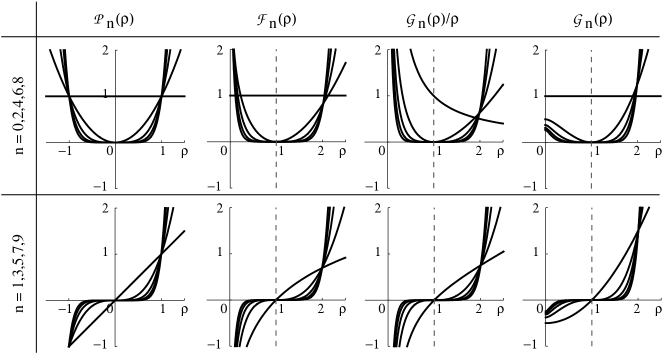
Figure 5: First five even (top row) and odd (bottom row) members of regular polynomials $\mathcal{P}_{n}=\rho^{n}$, $\mathcal{F}_{n}(\rho)$, $\frac{\mathcal{G}_{n}(\rho)}{\rho}$ and $\mathcal{G}_{n}(\rho)$ functions from the left to the right respectively.

First ten members of $\mathcal{F}_{n}$ and $\mathcal{G}_{n}$ are listed in Tables 6, 7 and are shown in FIG. 5; in Appendix B one can find Taylor series of these functions at $\rho=1$. The difference relation for $\mathcal{F}_{n}$ including first members have been found by E.M. McMillan and I would like to acknowledge his result by given them a name of McMillan radial harmonics. In addition to his results, adjoint McMillan radial harmonics, $\mathcal{G}_{n}$, are introduced in order to provide the symmetry in description between electric and magnetic fields.

Finally, in order to define the set of functions for pure S-multipoles (Table 5) we will define sector harmonics:

$$\mathcal{A}_{n}^{(\text{e})}(\rho,y) = \sum_{k=0}^{n}\begin{pmatrix}n\\ k\end{pmatrix}\mathcal{F}_{n-k}(\rho)\,y^{k}\cos\frac{k\,\pi}{2},$$

$$\mathcal{A}_{n}^{(\text{m})}(\rho,y) = \sum_{k=0}^{n}\begin{pmatrix}n\\ k\end{pmatrix}\frac{\mathcal{G}_{n-k}(\rho)}{\rho}\,y^{k}\cos\frac{k\,\pi}{2},$$

$$\mathcal{B}_{n}^{(\text{e})}(\rho,y) = \sum_{k=0}^{n}\begin{pmatrix}n\\ k\end{pmatrix}\mathcal{F}_{n-k}(\rho)\,y^{k}\sin\frac{k\,\pi}{2},$$

$$\mathcal{B}_{n}^{(\text{m})}(\rho,y) = \sum_{k=0}^{n}\begin{pmatrix}n\\ k\end{pmatrix}\frac{\mathcal{G}_{n-k}(\rho)}{\rho}\,y^{k}\sin\frac{k\,\pi}{2}.$$

obeying differential relations

$$n\,\{\mathcal{A,B}\}_{n-1}^{(\text{e}\,)} = \pm\frac{\partial\,\{\mathcal{B,A}\}_{n}^{(\text{e})}}{\partial y}=\frac{1}{\rho}\frac{\partial\left(\rho\,\{\mathcal{A,B}\}_{n}^{(\text{m})}\right)}{\partial\rho},$$

$$n\,\{\mathcal{A,B}\}_{n-1}^{(\text{m})} = \pm\frac{1}{\bcancel{\rho}}\frac{\partial\,\left(\bcancel{\rho}\,\{\mathcal{B,A}\}_{n}^{(\text{m})}\right)}{\partial y}=\frac{\partial\,\{\mathcal{A,B}\}_{n}^{(\text{e})}}{\partial\rho}.$$

Figure 6 shows the cross section of idealized multipole magnet’s poles and corresponding fields. First six members of spherical harmonics are listed in Table 8 and exact expressions for potentials and fields in Appendix A.

Table 5: Formulas for the scalar potential, azimuthal component of the vector potential and field components for “pure normal and skew $2n$-poles in cylindrical coordinates.

Normal	Skew
$\displaystyle\overline{\Phi}^{(n)}=-\overline{C}_{n}\frac{\mathcal{B}_{n}^{(\text{e})}}{n!}$	$\displaystyle\underline{\Phi}^{(n)}=-\underline{C}_{\,n}\frac{\mathcal{A}_{n}^{(\text{e})}}{n!}$
$\displaystyle\overline{A}_{\theta}^{(n)}=-\overline{C}_{n}\frac{\mathcal{A}_{n}^{(\text{m})}}{n!}$	$\displaystyle\underline{A}_{\,\theta}^{(n)}=\quad\!\!\underline{C}_{\,n}\frac{\mathcal{B}_{n}^{(\text{m})}}{n!}$
$\displaystyle\overline{F}_{\,\rho}^{(n)}=\quad\!\!\overline{C}_{n}\frac{\mathcal{B}_{n-1}^{\text{(m)}}}{(n-1)!}$	$\displaystyle\underline{F}_{\,\rho}^{(n)}=\quad\!\!\underline{C}_{\,n}\frac{\mathcal{A}_{n-1}^{\text{(m)}}}{(n-1)!}$
$\displaystyle\overline{F}_{\,\text{y}}^{(n)}=\quad\!\!\overline{C}_{n}\frac{\mathcal{A}_{n-1}^{\text{(e)}}}{(n-1)!}$	$\displaystyle\underline{F}_{\,\text{y}}^{(n)}=-\underline{C}_{\,n}\frac{\mathcal{B}_{n-1}^{\text{(e)}}}{(n-1)!}$

Table 6: First ten members of $\mathcal{F}-$functions.

$n$	$\mathcal{F}_{n}(\rho)$
0	$\displaystyle 1$
1	$\displaystyle\ln\rho$
2	$\displaystyle\frac{1}{2}\,(\rho^{2}-1)-\ln\rho$
3	$\displaystyle\frac{3}{2}\left[-(\rho^{2}-1)+(\rho^{2}+1)\ln\rho\phantom{\frac{1}{1}}\!\!\!\!\right]$
4	$\displaystyle\,3\,\left[\frac{1}{8}(\rho^{4}-1)+\frac{1}{2}(\rho^{2}-1)-\left(\rho^{2}+\frac{1}{2}\right)\ln\rho\right]$
5	$\displaystyle\frac{15}{2}\left[-\frac{3}{8}\left(\rho^{4}-1\right)+\left(\frac{1}{4}\,\rho^{4}+\rho^{2}+\frac{1}{4}\right)\ln\rho\right]$
6	$\displaystyle\frac{45}{4}\left[\frac{1}{36}\left(\rho^{6}-1\right)+\frac{1}{2}\left(\rho^{4}-1\right)-\frac{1}{4}\left(\rho^{2}-1\right)-\left(\frac{1}{2}\,\rho^{4}+\rho^{2}+\frac{1}{6}\right)\ln\rho\right]$
7	$\displaystyle\frac{315}{16}\left[-\frac{11}{54}\left(\rho^{6}-1\right)-\frac{1}{2}\,\rho^{2}\left(\rho^{2}-1\right)+\left\{\frac{1}{9}\left(\rho^{6}+1\right)+\rho^{2}\left(\rho^{2}+1\right)\right\}\ln\rho\right]$
8	$\displaystyle\frac{105}{4}\left[\frac{1}{96}\left(\rho^{8}-1\right)+\frac{4}{9}\left(\rho^{6}-1\right)+\frac{3}{8}\left(\rho^{4}-1\right)-\frac{2}{3}\left(\rho^{2}-1\right)-\left(\frac{1}{3}\,\rho^{6}+\frac{3}{2}\,\rho^{4}+\rho^{2}+\frac{1}{12}\right)\ln\rho\right]$
9	$\displaystyle\frac{315}{8}\left[-\frac{25}{192}\left(\rho^{8}-1\right)-\frac{5}{6}\,\rho^{2}\left(\rho^{4}-1\right)+\left\{\frac{1}{16}+\rho^{2}\left(\frac{\rho^{2}}{2}+1\right)\left(\frac{1}{8}\,\rho^{4}+\frac{7}{4}\,\rho^{2}+1\right)\right\}\ln\rho\right]$

Table 7: First ten members of $\mathcal{G}-$functions.

$n$	$\mathcal{G}_{n}(\rho)$
0	$\displaystyle 1$
1	$\displaystyle\frac{1}{2}\,(\rho^{2}-1)$
2	$\displaystyle\,1\,\!\left[-\frac{1}{2}\,(\rho^{2}-1)+\rho^{2}\ln\rho\right]$
3	$\displaystyle\frac{3}{2}\left[\frac{1}{4}\,(\rho^{4}-1)-\rho^{2}\ln\rho\right]$
4	$\displaystyle\,3\,\left[-\frac{5}{8}\,(\rho^{4}-1)+\frac{1}{2}(\rho^{2}-1)+\rho^{2}\left(\frac{\rho^{2}}{2}+1\right)\ln\rho\right]$
5	$\displaystyle\frac{15}{4}\left[\frac{1}{12}\,\left(\rho^{6}-1\right)+\frac{3}{4}\,\rho^{2}\left(\rho^{2}-1\right)-\rho^{2}\left(\rho^{2}+1\right)\ln\rho\right]$
6	$\displaystyle\frac{45}{8}\left[-\frac{5}{9}\,\left(\rho^{6}-1\right)-\frac{1}{2}\,\left(\rho^{4}-1\right)+\left(\rho^{2}-1\right)+\rho^{2}\left(\frac{1}{3}\,\rho^{4}+2\,\rho^{2}+1\right)\ln\rho\right]$
7	$\displaystyle\frac{105}{16}\left[\frac{1}{24}\,\left(\rho^{8}-1\right)+\frac{7}{6}\,\rho^{2}\left(\rho^{4}-1\right)-\left(\rho^{6}+3\,\rho^{4}+\rho^{2}\right)\ln\rho\right]$
8	$\displaystyle\,\,\frac{35}{4}\,\left[-\frac{47}{96}\,\left(\rho^{8}-1\right)-2\,\left(\rho^{6}-1\right)+\frac{9}{8}\,\left(\rho^{4}-1\right)+\frac{4}{3}\,\left(\rho^{2}-1\right)+\rho^{2}\left(\frac{1}{4}\,\rho^{6}+3\,\rho^{4}+\frac{9}{2}\,\rho^{2}+1\right)\ln\rho\right]$
9	$\displaystyle\frac{315}{32}\left[\frac{1}{40}\,\left(\rho^{10}-1\right)+\frac{35}{24}\,\rho^{2}\left(\rho^{6}-1\right)+\frac{5}{2}\,\rho^{4}\left(\rho^{2}-1\right)-\left(\rho^{8}+6\,\rho^{6}+6\,\rho^{4}+\rho^{2}\right)\ln\rho\right]$

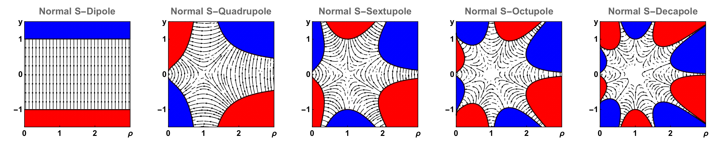
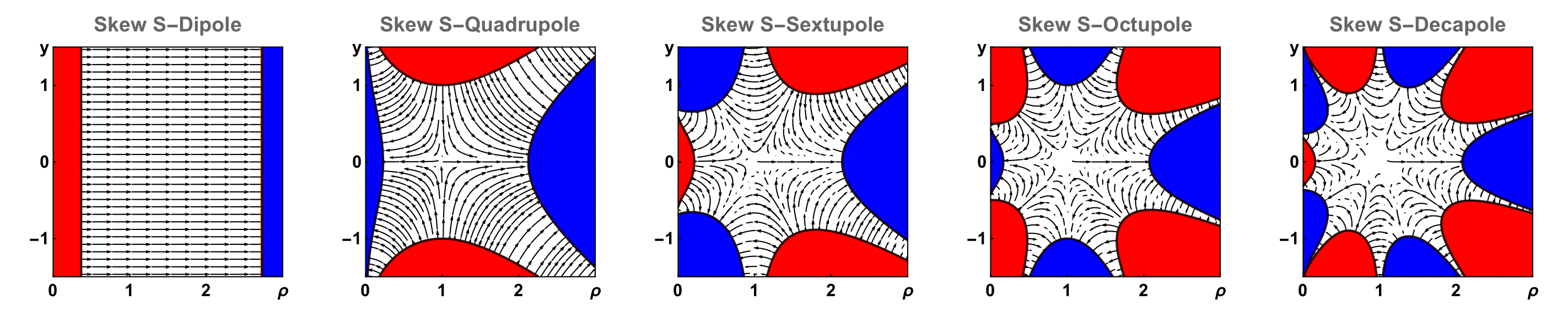
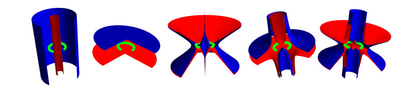
Figure 6: Normal and skew 2n-pole magnets in cylindrical coordinates. Each figure shows magnetic (electric) field streamlines and poles’ shape in transverse cross section. North (positive electrostatic potential) and south (negative electrostatic potential) poles are shown in red and blue and given by constant levels of $(\mathcal{B,A})_{n}^{\text{(e)}}=\mp\text{const}$ respectively, $\text{const}=1$ for this example. Bottom row shows 3D models of sector magnets with $\theta=3\pi/2$: skew S-dipole, normal S-dipole, skew S-quadrupole, normal S-quadrupole and skew S-sextupole from the left to the right respectively. Equilibrium orbit is shown in green color

Table 8: Sector harmonics.

	n
$\mathcal{A}_{n}^{(\text{e})}$	0	$\displaystyle 1\phantom{\left[\frac{1}{1}\right]}$
	1	$\displaystyle\ln\rho\phantom{\left[\frac{1}{1}\right]}$
	2	$\displaystyle\left[\frac{\rho^{2}-1}{2}-y^{2}\right]-\ln\rho$
	3	$\displaystyle\left[-3\,\frac{\rho^{2}-1}{2}\right]+3\,\left(\frac{\rho^{2}+1}{2}-y^{2}\right)\ln\rho$
	4	$\displaystyle\left[\frac{3(\rho^{4}+4\,\rho^{2}-5)}{8}-6\,\frac{\rho^{2}-1}{2}\,y^{2}+y^{4}\right]-3\,\left(\frac{1}{2}+\rho^{2}-2\,y^{2}\right)\,\ln\rho$
	5	$\displaystyle\left[-5\,\frac{9\,(\rho^{4}-1)}{16}+5\times 6\frac{\rho^{2}-1}{2}\,y^{2}\right]+5\,\left(\frac{3(\rho^{4}+4\,\rho^{2}+1)}{8}-6\,\frac{\rho^{2}+1}{2}\,y^{2}+y^{4}\right)\ln\rho$
$\mathcal{A}_{n}^{(\text{m})}$	0	$\displaystyle\frac{1}{\rho}\left\{1\phantom{\frac{1}{1}}\!\!\!\!\right\}$
	1	$\displaystyle\frac{1}{\rho}\left\{\left[\frac{\rho^{2}-1}{2}\right]\right\}$
	2	$\displaystyle\frac{1}{\rho}\left\{\left[-\frac{\rho^{2}-1}{2}-y^{2}\right]+\rho^{2}\ln\rho\right\}$
	3	$\displaystyle\frac{1}{\rho}\left\{\left[\frac{3(\rho^{2}+1)}{4}\frac{\rho^{2}-1}{2}-3\,\frac{\rho^{2}-1}{2}\,y^{2}\right]-\frac{3}{2}\,\rho^{2}\ln\rho\right\}$
	4	$\displaystyle\frac{1}{\rho}\left\{\left[-\frac{3(5\,\rho^{4}-4\,\rho^{2}-1)}{8}+6\,\frac{\rho^{2}-1}{2}\,y^{2}+y^{4}\right]+\frac{3(2+\rho^{2}-4\,y^{2})}{2}\,\rho^{2}\ln\rho\right\}$
	5	$\displaystyle\frac{1}{\rho}\left\{\left[\frac{5(\rho^{4}+10\,\rho^{2}+1)}{8}\frac{\rho^{2}-1}{2}-10\,\frac{3(\rho^{2}+1)}{4}\frac{\rho^{2}-1}{2}\,y^{2}+5\,\frac{\rho^{2}-1}{2}\,y^{4}\right]-\frac{15(1+\rho^{2}-4\,y^{2})}{4}\,\rho^{2}\ln\rho\right\}$
$\mathcal{B}_{n}^{(\text{e})}$	0	$\displaystyle 0\phantom{\frac{1}{1}}$
	1	$\displaystyle y\left\{\!\!\!\!\!\!\!\!\!\!\!\phantom{\left[\frac{1}{1}\right]}1\right\}$
	2	$\displaystyle y\left\{\!\!\!\!\!\!\!\!\!\!\!\phantom{\left[\frac{1}{1}\right]}2\,\ln\rho\right\}$
	3	$\displaystyle y\left\{\left[3\,\frac{\rho^{2}-1}{2}-y^{2}\right]-3\,\ln\rho\right\}$
	4	$\displaystyle y\left\{\left[-12\,\frac{\rho^{2}-1}{2}\right]+4\,\left(3\,\frac{\rho^{2}+1}{2}-y^{2}\right)\ln\rho\right\}$
	5	$\displaystyle y\left\{\left[5\,\frac{3\,(\rho^{4}+4\,\rho^{2}-5)}{8}-10\,\frac{\rho^{2}-1}{2}\,y^{2}+y^{4}\right]-5\left(\frac{3}{2}+3\,\rho^{2}-2\,y^{2}\right)\ln\rho\right\}$
$\mathcal{B}_{n}^{(\text{m})}$	0	$\,\displaystyle 0\phantom{\frac{1}{1}}$
	1	$\displaystyle\frac{y}{\rho}\left\{\!\!\!\!\!\!\!\!\!\!\!\phantom{\left[\frac{1}{1}\right]}1\right\}$
	2	$\displaystyle\frac{y}{\rho}\left\{\left[2\,\frac{\rho^{2}-1}{2}\right]\right\}$
	3	$\displaystyle\frac{y}{\rho}\left\{\left[-3\,\frac{\rho^{2}-1}{2}-y^{2}\right]+3\,\rho^{2}\ln\rho\right\}$
	4	$\displaystyle\frac{y}{\rho}\left\{\left[4\,\frac{3(\rho^{2}+1)}{4}\frac{\rho^{2}-1}{2}-4\,\frac{\rho^{2}-1}{2}\,y^{2}\right]-6\,\rho^{2}\ln\rho\right\}$
	5	$\displaystyle\frac{y}{\rho}\left\{\left[-5\,\frac{3(5\,\rho^{4}-4\,\rho^{2}-1)}{8}+10\,\frac{\rho^{2}-1}{2}\,y^{2}+y^{4}\right]+5\,\left(3+\frac{3}{2}\,\rho^{2}-2\,y^{2}\right)\rho^{2}\ln\rho\right\}$

III.6 Recurrence equations in sector coordinates

An alternative approach to find expansions for potentials is to use general power series ansatz. In Cartesian coordinates the use of

$$\Phi=-\sum_{m,n\geq 0}^{\infty}V_{m,n}\frac{x^{m}}{m!}\frac{y^{n}}{n!}$$

gives the recurrence relation

$$V_{m+2,n}+V_{m,n+2}=0.$$

This equation immediately defines all coefficients, and up to a common factor, as easy to see, coincides with harmonic homogeneous polynomials $\mathcal{A}_{n}$ and $\mathcal{B}_{n}$.

In sector coordinates, the same substitution for $\Phi$, and

$$A_{\theta}=-\sum_{m,n\geq 0}^{\infty}\frac{1}{1+x}V_{m,n}\frac{x^{m}}{m!}\frac{y^{n}}{n!}$$

substitution for longitudinal component of the vector potential gives two new recurrences, respectively

$$V_{m+2,n}+V_{m,n+2}=-(m\pm 1)\,V_{m+1.n}-m\,V_{m-1,n+2}.$$

The detailed approach on how to treat these equations can be found for example in [Wiedemann]. In order to solve these recurrences, one can look for a solution where each term can be expressed in a form

$$V_{i,j}=V_{i,j}^{*}+V_{i,j}^{(i+j-1)}+V_{i,j}^{(i+j-2)}+V_{i,j}^{(i+j-3)}+\ldots$$

where starred variables are the “design” terms given by pure multipole fields and thus satisfying

$$V_{m+2,n}^{*}+V_{m,n+2}^{*}\equiv 0.$$

Other coefficients $V_{i,j}^{(k)}$ are terms induced by lower $k$-th order pure multipoles due to recurrence. Thus in order to find an expression for a particular $2n$-pole we will start the recurrence form the $n$-th order assuming that

$$V_{n,0}=-V_{n-2,2}=\ldots\quad\text{or}\quad V_{n-1,1}=-V_{n-3,3}=\ldots$$

for normal and skew elements. Then we will start exploiting the recurrence where all terms in the form $V_{i,j}^{(n)}$ for $i+j>n$ are subject to be determined.

This approach has two major disadvantages. At first, in order to use the result on will have to truncate a recurrence. As a result the potentials representing magnets do not satisfies the Laplace equation anymore. This is a strong assumption which violate the “physics” and should be avoided. While potentials can be approximated with any precision by keeping an appropriate number of terms, there is another issue. At second, at each new order when solving the recurrence one will find that an arbitrary constant $\alpha_{i}\in(0;1)$ should be introduced since the system is undetermined. An additional assumption $(A_{s},\Phi)\left.\right|_{x=0}\propto y^{n}$ allows to truncate or summate the series. The resulting solutions coincide with the one obtained above.

IV Summary

The scalar and vector Laplace’s equations for static transverse electromagnetic fields in curvilinear orthogonal coordinates with zero and constant curvature are solved. In Cartesian coordinates these solutions are well known harmonic homogeneous polynomials of two variables. The set of solutions in cylindrical coordinates named sector harmonics, and should not be confused with cylindrical harmonics where $\rho$-dependent term is given by Bessel functions which occasionally are also called cylindrical harmonics. In contrast, the radial part is given by the set of introduced McMillan radial harmonics, independently introduced by E.M. McMillan in his “forgotten” article, and adjoint radial harmonics also described in this work. The feature of sector harmonics that when expanded around equilibrium orbit they resemble solution in Cartesian geometry. Compared to the traditional approach, widely used in accelerator community, of the use of recurrences based on general power series ansatz, this set of functions has two major advantages. It do not require any truncation and is exactly satisfying Laplace equation, and, provides a well defined full basis of functions which can be related to any field by its expansion in radial or vertical planes, see Table 9. Including the model Hamiltonians for $t$- and $s$-representations, where no assumptions but the field symmetry has been used, one can construct numerical scheme integrating equations of motion. Thus I would like to suggest the set of sector harmonics as a new basis for description and design of any sector magnets with translational symmetry along azimuthal coordinate.

Table 9: Relationship between coefficients determining the strength of “pure” normal and skew S-multipoles and power series expansion of field in radial and vertical planes on equilibrium orbit.

	$n$	$x=0$	$y=0$
$\overline{C}_{n}$	1	$F_{y}$	$F_{y}$
	2	$\partial_{y}\,F_{x}$	$\partial_{x}\,F_{y}$
	3	$-\partial_{y}^{2}\,F_{y}$	$\partial_{x}^{2}\,F_{y}+\partial_{x}\,F_{y}$
	4	$-\partial_{y}^{3}\,F_{x}$	$\partial_{x}^{3}\,F_{y}+\partial_{x}^{2}\,F_{y}-\partial_{x}\,F_{y}$
	5	$\partial_{y}^{4}\,F_{y}$	$\partial_{x}^{4}\,F_{y}+2\,\partial_{x}^{3}\,F_{y}-\partial_{x}^{2}\,F_{y}+\partial_{x}\,F_{y}$
	6	$\partial_{y}^{5}\,F_{x}$	$\partial_{x}^{5}\,F_{y}+2\,\partial_{x}^{4}\,F_{y}-3\,\partial_{x}^{3}\,F_{y}+3\,\partial_{x}^{2}\,F_{y}-3\,\partial_{x}\,F_{y}$
	7	$-\partial_{y}^{6}\,F_{y}$	$\partial_{x}^{6}\,F_{y}+3\,\partial_{x}^{5}\,F_{y}-3\,\partial_{x}^{4}\,F_{y}+6\,\partial_{x}^{3}\,F_{y}-9\,\partial_{x}^{2}\,F_{y}+9\,\partial_{x}\,F_{y}$
	8	$-\partial_{y}^{7}\,F_{x}$	$\partial_{x}^{7}\,F_{y}+3\,\partial_{x}^{6}\,F_{y}-6\,\partial_{x}^{5}\,F_{y}+12\,\partial_{x}^{4}\,F_{y}-27\,\partial_{x}^{3}\,F_{y}+45\,\partial_{x}^{2}\,F_{y}-45\,\partial_{x}\,F_{y}$
	9	$\partial_{y}^{8}\,F_{y}$	$\partial_{x}^{8}\,F_{y}+4\,\partial_{x}^{7}\,F_{y}-6\,\partial_{x}^{6}\,F_{y}+18\,\partial_{x}^{5}\,F_{y}-51\,\partial_{x}^{4}\,F_{y}+126\,\partial_{x}^{3}\,F_{y}-225\,\partial_{x}^{2}\,F_{y}+225\,\partial_{x}\,F_{y}$
$\underline{C}_{\,n}$	1	$F_{x}$	$F_{x}$
	2	$-\partial_{y}\,F_{y}$	$\partial_{x}\,F_{x}+F_{x}$
	3	$-\partial_{y}^{2}\,F_{x}$	$\partial_{x}^{2}\,F_{x}+\partial_{x}\,F_{x}-F_{x}$
	4	$\partial_{y}^{3}\,F_{y}$	$\partial_{x}^{3}\,F_{x}+2\,\partial_{x}^{2}\,F_{x}-\partial_{x}\,F_{x}+F_{x}$
	5	$\partial_{y}^{4}\,F_{x}$	$\partial_{x}^{4}\,F_{x}+2\,\partial_{x}^{3}\,F_{x}-3\,\partial_{x}^{2}\,F_{x}+3\,\partial_{x}\,F_{x}-3\,F_{x}$
	6	$-\partial_{y}^{5}\,F_{y}$	$\partial_{x}^{5}\,F_{x}+3\,\partial_{x}^{4}\,F_{x}-3\,\partial_{x}^{3}\,F_{x}+6\,\partial_{x}^{2}\,F_{x}-9\,\partial_{x}\,F_{x}+9\,F_{x}$
	7	$-\partial_{y}^{6}\,F_{x}$	$\partial_{x}^{6}\,F_{x}+3\,\partial_{x}^{5}\,F_{x}-6\,\partial_{x}^{4}\,F_{x}+12\,\partial_{x}^{3}\,F_{x}-27\,\partial_{x}^{2}\,F_{x}+45\,\partial_{x}\,F_{x}-45\,F_{x}$
	8	$\partial_{y}^{7}\,F_{y}$	$\partial_{x}^{7}\,F_{x}+4\,\partial_{x}^{6}\,F_{x}-6\,\partial_{x}^{5}\,F_{x}+18\,\partial_{x}^{4}\,F_{x}-51\,\partial_{x}^{3}\,F_{x}+126\,\partial_{x}^{2}\,F_{x}-225\,\partial_{x}\,F_{x}+225\,F_{x}$
	9	$\partial_{y}^{8}\,F_{x}$	$\partial_{x}^{8}\,F_{x}+4\,\partial_{x}^{7}\,F_{x}-10\,\partial_{x}^{6}\,F_{x}+30\,\partial_{x}^{5}\,F_{x}-105\,\partial_{x}^{4}\,F_{x}+330\,\partial_{x}^{3}\,F_{x}-855\,\partial_{x}^{2}\,F_{x}+1575\,\partial_{x}\,F_{x}-1575\,F_{x}$

Appendix A R- ans S- multipoles. Exact expressions.

The scalar potentials, longitudinal component of vector potential, and field components for pure R- and S-multipoles up to fifth order are listed in Table 10–11 and Tables 12–13 respectively.

Appendix B Taylor polynomials of $\mathcal{F}_{n}$ and $\mathcal{G}_{n}$.

The first ten terms of Maclaurin series of $\mathcal{F}_{n}(x)$, $\mathcal{G}_{n}(x)$ and $\displaystyle\frac{\mathcal{G}_{n}(x)}{1+x}$ are listed in Table 14.

Table 10: Longitudinal component of the vector potential and scalar potential for pure normal and skew R-multipoles.

$n$		$A_{z}$	$\Phi$
0	calibration	$\displaystyle-\,\overline{C}_{0}$	$\,\,\,\,\,\,0$
1	normal dipole	$\displaystyle-\frac{1}{1!}(x)\,\overline{C}_{1}$	$\displaystyle-\frac{1}{1!}(y)\,\overline{C}_{1}$
2	normal quadrupole	$\displaystyle-\frac{1}{2!}(x^{2}-y^{2})\,\overline{C}_{2}$	$\displaystyle-\frac{1}{2!}(2\,x\,y)\,\overline{C}_{2}$
3	normal sextupole	$\displaystyle-\frac{1}{3!}(x^{3}-3\,x\,y^{2})\,\overline{C}_{3}$	$\displaystyle-\frac{1}{3!}(3\,x^{2}y-y^{3})\,\overline{C}_{3}$
4	normal octupole	$\displaystyle-\frac{1}{4!}(x^{4}-6\,x^{2}y^{2}+y^{4})\,\overline{C}_{4}$	$\displaystyle-\frac{1}{4!}(4\,x^{3}y-4\,x\,y^{3})\,\overline{C}_{4}$
5	normal decapole	$\displaystyle-\frac{1}{5!}(x^{5}-10\,x^{3}y^{2}+5\,x\,y^{4})\,\overline{C}_{5}$	$\displaystyle-\frac{1}{5!}(5\,x^{4}y-10\,x^{2}y^{3}+y^{5})\,\overline{C}_{5}$
0	calibration	$\,\,\,\,\,0$	$\,\,\,\,\,\underline{C}_{\,0}$
1	skew dipole	$\,\,\,\,\displaystyle\frac{1}{1!}(y)\,\underline{C}_{\,1}$	$\displaystyle-\frac{1}{1!}(x)\,\underline{C}_{\,1}$
2	skew quadrupole	$\,\,\,\,\displaystyle\frac{1}{2!}(2\,x\,y)\,\underline{C}_{\,2}$	$\displaystyle-\frac{1}{2!}(x^{2}-y^{2})\,\underline{C}_{\,2}$
3	skew sextupole	$\,\,\,\,\displaystyle\frac{1}{3!}(3\,x^{2}y-y^{3})\,\underline{C}_{\,3}$	$\displaystyle-\frac{1}{3!}(x^{3}-3\,x\,y^{2})\,\underline{C}_{\,3}$
4	skew octupole	$\,\,\,\,\displaystyle\frac{1}{4!}(4\,x^{3}y-4\,x\,y^{3})\,\underline{C}_{\,4}$	$\displaystyle-\frac{1}{4!}(x^{4}-6\,x^{2}y^{2}+y^{4})\,\underline{C}_{\,4}$
5	skew decapole	$\,\,\,\,\displaystyle\frac{1}{5!}(5\,x^{4}y-10\,x^{2}y^{3}+y^{5})\,\underline{C}_{\,5}$	$\displaystyle-\frac{1}{5!}(x^{5}-10\,x^{3}y^{2}+5\,x\,y^{4})\,\underline{C}_{\,5}$

Table 11: Horizontal and vertical components of pure normal and skew R-multipole magnets’ field.

$n$		$F_{x}$	$F_{y}$
0	calibration	—	—
1	normal dipole	$\,0$	$\,\,\,\,\,\overline{C}_{1}$
2	normal quadrupole	$\displaystyle\frac{1}{1!}(y)\,\overline{C}_{2}$	$\,\,\,\,\displaystyle\frac{1}{1!}(x)\,\overline{C}_{2}$
3	normal sextupole	$\displaystyle\frac{1}{2!}(2\,x\,y)\,\overline{C}_{3}$	$\,\,\,\,\displaystyle\frac{1}{2!}(x^{2}-y^{2})\,\overline{C}_{3}$
4	normal octupole	$\displaystyle\frac{1}{3!}(3\,x^{2}y-y^{3})\,\overline{C}_{4}$	$\,\,\,\,\displaystyle\frac{1}{3!}(x^{3}-3\,x\,y^{2})\,\overline{C}_{4}$
5	normal decapole	$\displaystyle\frac{1}{4!}(4\,x^{3}y-4\,x\,y^{3})\,\overline{C}_{5}$	$\,\,\,\,\displaystyle\frac{1}{4!}(x^{4}-6\,x^{2}y^{2}+y^{4})\,\overline{C}_{5}$
0	calibration	—	—
1	skew dipole	$\,\underline{C}_{\,1}$	$\,\,\,\,\,\,0$
2	skew quadrupole	$\displaystyle\frac{1}{1!}(x)\,\underline{C}_{\,2}$	$\displaystyle-\frac{1}{1!}(y)\,\underline{C}_{\,2}$
3	skew sextupole	$\displaystyle\frac{1}{2!}(x^{2}-y^{2})\,\underline{C}_{\,3}$	$\displaystyle-\frac{1}{2!}(2\,x\,y)\,\underline{C}_{\,3}$
4	skew octupole	$\displaystyle\frac{1}{3!}(x^{3}-3\,x\,y^{2})\,\underline{C}_{\,4}$	$\displaystyle-\frac{1}{3!}(3\,x^{2}y-y^{3})\,\underline{C}_{\,4}$
5	skew decapole	$\displaystyle\frac{1}{4!}(x^{4}-6\,x^{2}y^{2}+y^{4})\,\underline{C}_{\,5}$	$\displaystyle-\frac{1}{4!}(4\,x^{3}y-4\,x\,y^{3})\,\underline{C}_{\,5}$

Table 12: Azimuthal component of the vector potential and scalar potential for “pure” normal and skew S-multipoles.

	n
$\overline{A}_{\theta}^{(n)}$	0	$\displaystyle-\frac{1}{0!}\frac{1}{\rho}\left\{1\phantom{\frac{1}{1}}\!\!\!\!\right\}\,\overline{C}_{0}$
	1	$\displaystyle-\frac{1}{1!}\frac{1}{\rho}\left\{\left[\frac{\rho^{2}-1}{2}\right]\right\}\,\overline{C}_{1}$
	2	$\displaystyle-\frac{1}{2!}\frac{1}{\rho}\left\{\left[-\frac{\rho^{2}-1}{2}-y^{2}\right]+\rho^{2}\ln\rho\right\}\,\overline{C}_{2}$
	3	$\displaystyle-\frac{1}{3!}\frac{1}{\rho}\left\{\left[\frac{3(\rho^{2}+1)}{4}\frac{\rho^{2}-1}{2}-3\,\frac{\rho^{2}-1}{2}\,y^{2}\right]-\frac{3}{2}\,\rho^{2}\ln\rho\right\}\,\overline{C}_{3}$
	4	$\displaystyle-\frac{1}{4!}\frac{1}{\rho}\left\{\left[-\frac{3(5\,\rho^{4}-4\,\rho^{2}-1)}{8}+6\,\frac{\rho^{2}-1}{2}\,y^{2}+y^{4}\right]+\frac{3(2+\rho^{2}-4\,y^{2})}{2}\,\rho^{2}\ln\rho\right\}\,\overline{C}_{4}$
	5	$\displaystyle-\frac{1}{5!}\frac{1}{\rho}\left\{\left[\frac{5(\rho^{4}+10\,\rho^{2}+1)}{8}\frac{\rho^{2}-1}{2}-10\,\frac{3(\rho^{2}+1)}{4}\frac{\rho^{2}-1}{2}\,y^{2}+5\,\frac{\rho^{2}-1}{2}\,y^{4}\right]-\frac{15(1+\rho^{2}-4\,y^{2})}{4}\,\rho^{2}\ln\rho\right\}\,\overline{C}_{5}$
$\overline{\Phi}^{(n)}$	0	$\quad\displaystyle 0\phantom{\frac{1}{1}}$
	1	$\displaystyle-\frac{1}{1!}\,y\left\{\!\!\!\!\!\!\!\!\!\!\!\phantom{\left[\frac{1}{1}\right]}1\right\}\,\overline{C}_{1}$
	2	$\displaystyle-\frac{1}{2!}\,y\left\{\!\!\!\!\!\!\!\!\!\!\!\phantom{\left[\frac{1}{1}\right]}2\,\ln\rho\right\}\,\overline{C}_{2}$
	3	$\displaystyle-\frac{1}{3!}\,y\left\{\left[3\,\frac{\rho^{2}-1}{2}-y^{2}\right]-3\,\ln\rho\right\}\,\overline{C}_{3}$
	4	$\displaystyle-\frac{1}{4!}\,y\left\{\left[-12\,\frac{\rho^{2}-1}{2}\right]+4\,\left(3\,\frac{\rho^{2}+1}{2}-y^{2}\right)\ln\rho\right\}\,\overline{C}_{4}$
	5	$\displaystyle-\frac{1}{5!}\,y\left\{\left[5\,\frac{3\,(\rho^{4}+4\,\rho^{2}-5)}{8}-10\,\frac{\rho^{2}-1}{2}\,y^{2}+y^{4}\right]-5\left(\frac{3}{2}+3\,\rho^{2}-2\,y^{2}\right)\ln\rho\right\}\,\overline{C}_{5}$
$\underline{A}_{\,\theta}^{(n)}$	0	$\quad\!\,\displaystyle 0\phantom{\frac{1}{1}}$
	1	$\quad\!\displaystyle\frac{1}{1!}\frac{y}{\rho}\left\{\!\!\!\!\!\!\!\!\!\!\!\phantom{\left[\frac{1}{1}\right]}1\right\}\,\underline{C}_{\,1}$
	2	$\quad\!\displaystyle\frac{1}{2!}\frac{y}{\rho}\left\{\left[2\,\frac{\rho^{2}-1}{2}\right]\right\}\,\underline{C}_{\,2}$
	3	$\quad\!\displaystyle\frac{1}{3!}\frac{y}{\rho}\left\{\left[-3\,\frac{\rho^{2}-1}{2}-y^{2}\right]+3\,\rho^{2}\ln\rho\right\}\,\underline{C}_{\,3}$
	4	$\quad\!\displaystyle\frac{1}{4!}\frac{y}{\rho}\left\{\left[4\,\frac{3(\rho^{2}+1)}{4}\frac{\rho^{2}-1}{2}-4\,\frac{\rho^{2}-1}{2}\,y^{2}\right]-6\,\rho^{2}\ln\rho\right\}\,\underline{C}_{\,4}$
	5	$\quad\!\displaystyle\frac{1}{5!}\frac{y}{\rho}\left\{\left[-5\,\frac{3(5\,\rho^{4}-4\,\rho^{2}-1)}{8}+10\,\frac{\rho^{2}-1}{2}\,y^{2}+y^{4}\right]+5\,\left(3+\frac{3}{2}\,\rho^{2}-2\,y^{2}\right)\rho^{2}\ln\rho\right\}\,\underline{C}_{\,5}$
$\underline{\Phi}^{(n)}$	0	$\displaystyle-\frac{1}{0!}\left\{1\phantom{\frac{1}{1}}\!\!\!\!\!\right\}\,\underline{C}_{\,0}$
	1	$\displaystyle-\frac{1}{1!}\left\{\!\!\!\!\!\!\!\!\!\!\!\phantom{\left[\frac{1}{1}\right]}\ln\rho\phantom{\frac{1}{1}}\!\!\!\!\right\}\,\underline{C}_{\,1}$
	2	$\displaystyle-\frac{1}{2!}\left\{\left[\frac{\rho^{2}-1}{2}-y^{2}\right]-\ln\rho\right\}\,\underline{C}_{\,2}$
	3	$\displaystyle-\frac{1}{3!}\left\{\left[-3\,\frac{\rho^{2}-1}{2}\right]+3\,\left(\frac{\rho^{2}+1}{2}-y^{2}\right)\ln\rho\right\}\,\underline{C}_{\,3}$
	4	$\displaystyle-\frac{1}{4!}\left\{\left[\frac{3(\rho^{4}+4\,\rho^{2}-5)}{8}-6\,\frac{\rho^{2}-1}{2}\,y^{2}+y^{4}\right]-3\,\left(\frac{1}{2}+\rho^{2}-2\,y^{2}\right)\,\ln\rho\right\}\,\underline{C}_{\,4}$
	5	$\displaystyle-\frac{1}{5!}\left\{\left[-5\,\frac{9\,(\rho^{4}-1)}{16}+5\times 6\frac{\rho^{2}-1}{2}\,y^{2}\right]+5\,\left(\frac{3(\rho^{4}+4\,\rho^{2}+1)}{8}-6\,\frac{\rho^{2}+1}{2}\,y^{2}+y^{4}\right)\ln\rho\right\}\,\underline{C}_{\,5}$

Table 13: Radial and vertical components of “pure” normal and skew S-multipoles’ field.

	n
$\overline{F}_{\,\rho}^{(n)}$	0	calibration	—
	1	normal dipole	$\quad\displaystyle\,0\phantom{\frac{1}{1}}$
	2	normal quadrupole	$-\displaystyle\frac{1}{1!}\frac{y}{\rho}\left\{\!\!\!\!\!\!\!\!\!\!\!\phantom{\left[\frac{1}{1}\right]}1\right\}\,\overline{C}_{2}$
	3	normal sextupole	$-\displaystyle\frac{1}{2!}\frac{y}{\rho}\left\{\left[2\,\frac{\rho^{2}-1}{2}\right]\right\}\,\overline{C}_{3}$
	4	normal octupole	$-\displaystyle\frac{1}{3!}\frac{y}{\rho}\left\{\left[-3\,\frac{\rho^{2}-1}{2}-y^{2}\right]+3\,\rho^{2}\ln\rho\right\}\,\overline{C}_{4}$
	5	normal decapole	$-\displaystyle\frac{1}{4!}\frac{y}{\rho}\left\{\left[4\,\frac{3(\rho^{2}+1)}{4}\frac{\rho^{2}-1}{2}-4\,\frac{\rho^{2}-1}{2}\,y^{2}\right]-6\,\rho^{2}\ln\rho\right\}\,\overline{C}_{5}$
$\overline{F}_{\,\text{y}}^{(n)}$	0	calibration	—
	1	normal dipole	$\quad\!\displaystyle\frac{1}{0!}\left\{1\phantom{\frac{1}{1}}\!\!\!\!\!\right\}\,\overline{C}_{1}$
	2	normal quadrupole	$\quad\!\displaystyle\frac{1}{1!}\left\{\!\!\!\!\!\!\!\!\!\!\!\phantom{\left[\frac{1}{1}\right]}\ln\rho\phantom{\frac{1}{1}}\!\!\!\!\right\}\,\overline{C}_{2}$
	3	normal sextupole	$\quad\!\displaystyle\frac{1}{2!}\left\{\left[\frac{\rho^{2}-1}{2}-y^{2}\right]-\ln\rho\right\}\,\overline{C}_{3}$
	4	normal octupole	$\quad\!\displaystyle\frac{1}{3!}\left\{\left[-3\,\frac{\rho^{2}-1}{2}\right]+3\,\left(\frac{\rho^{2}+1}{2}-y^{2}\right)\ln\rho\right\}\,\overline{C}_{4}$
	5	normal decapole	$\quad\!\displaystyle\frac{1}{4!}\left\{\left[\frac{3(\rho^{4}+4\,\rho^{2}-5)}{8}-6\,\frac{\rho^{2}-1}{2}\,y^{2}+y^{4}\right]-3\,\left(\frac{1}{2}+\rho^{2}-2\,y^{2}\right)\,\ln\rho\right\}\,\overline{C}_{5}$
$\underline{F}_{\,\rho}^{(n)}$	0	calibration	—
	1	skew dipole	$\quad\!\displaystyle\frac{1}{0!}\frac{1}{\rho}\left\{1\phantom{\frac{1}{1}}\!\!\!\!\right\}\,\underline{C}_{\,1}$
	2	skew quadrupole	$\quad\!\displaystyle\frac{1}{1!}\frac{1}{\rho}\left\{\left[\frac{\rho^{2}-1}{2}\right]\right\}\,\underline{C}_{\,2}$
	3	skew sextupole	$\quad\!\displaystyle\frac{1}{2!}\frac{1}{\rho}\left\{\left[-\frac{\rho^{2}-1}{2}-y^{2}\right]+\rho^{2}\ln\rho\right\}\,\underline{C}_{\,3}$
	4	skew octupole	$\quad\!\displaystyle\frac{1}{3!}\frac{1}{\rho}\left\{\left[\frac{3(\rho^{2}+1)}{4}\frac{\rho^{2}-1}{2}-3\,\frac{\rho^{2}-1}{2}\,y^{2}\right]-\frac{3}{2}\,\rho^{2}\ln\rho\right\}\,\underline{C}_{\,4}$
	5	skew decapole	$\quad\!\displaystyle\frac{1}{4!}\frac{1}{\rho}\left\{\left[-\frac{3(5\,\rho^{4}-4\,\rho^{2}-1)}{8}+6\,\frac{\rho^{2}-1}{2}\,y^{2}+y^{4}\right]+\frac{3(2+\rho^{2}-4\,y^{2})}{2}\,\rho^{2}\ln\rho\right\}\,\underline{C}_{\,5}$
$\underline{F}_{\,\text{y}}^{(n)}$	0	calibration	—
	1	skew dipole	$\quad\displaystyle\,0\phantom{\frac{1}{1}}$
	2	skew quadrupole	$\quad\!\displaystyle\frac{1}{1!}\,y\left\{\!\!\!\!\!\!\!\!\!\!\!\phantom{\left[\frac{1}{1}\right]}1\right\}\,\underline{C}_{\,2}$
	3	skew sextupole	$\quad\!\displaystyle\frac{1}{2!}\,y\left\{\!\!\!\!\!\!\!\!\!\!\!\phantom{\left[\frac{1}{1}\right]}2\,\ln\rho\right\}\,\underline{C}_{\,3}$
	4	skew octupole	$\quad\!\displaystyle\frac{1}{3!}\,y\left\{\left[3\,\frac{\rho^{2}-1}{2}-y^{2}\right]-3\,\ln\rho\right\}\,\underline{C}_{\,4}$
	5	skew decapole	$\quad\!\displaystyle\frac{1}{4!}\,y\left\{\left[-12\,\frac{\rho^{2}-1}{2}\right]+4\,\left(3\,\frac{\rho^{2}+1}{2}-y^{2}\right)\ln\rho\right\}\,\underline{C}_{\,5}$

Table 14: Maclaurin series of $\mathcal{F}_{n}(x)$, $\mathcal{G}_{n}(x)$ and $\frac{\mathcal{G}_{n}(x)}{1+x}$; they are also Taylor polynomials of $\mathcal{F}_{n}(\rho)$, $\mathcal{G}_{n}(\rho)$ and $\frac{\mathcal{G}_{n}(\rho)}{\rho}$ at $\rho=1$.

$n$	$\mathrm{T}(\mathcal{F}_{n})$
0	$\displaystyle 1\phantom{\frac{1}{1}}$
1	$\displaystyle x-\frac{1}{2}\,x^{2}+\frac{1}{3}\,x^{3}-\frac{1}{4}\,x^{4}+\frac{1}{5}\,x^{5}-\frac{1}{6}\,x^{6}+\frac{1}{7}\,x^{7}-\frac{1}{8}\,x^{8}+\frac{1}{9}\,x^{9}-\frac{1}{10}\,x^{10}+O(x^{11})$
2	$\displaystyle x^{2}-\frac{1}{3}\,x^{3}+\frac{1}{4}\,x^{4}-\frac{1}{5}\,x^{5}+\frac{1}{6}\,x^{6}-\frac{1}{7}\,x^{7}+\frac{1}{8}\,x^{8}-\frac{1}{9}\,x^{9}+\frac{1}{10}\,x^{10}-\frac{1}{11}\,x^{11}+O(x^{12})$
3	$\displaystyle x^{3}-\frac{1}{2}\,x^{4}+\frac{7}{20}\,x^{5}-\frac{11}{40}\,x^{6}+\frac{8}{35}\,x^{7}-\frac{11}{56}\,x^{8}+\frac{29}{168}\,x^{9}-\frac{37}{240}\,x^{10}+\frac{23}{165}\,x^{11}-\frac{7}{55}\,x^{12}+O(x^{13})$
4	$\displaystyle x^{4}-\frac{2}{5}\,x^{5}+\frac{3}{10}\,x^{6}-\frac{17}{70}\,x^{7}+\frac{23}{112}\,x^{8}-\frac{5}{28}\,x^{9}+\frac{19}{120}\,x^{10}-\frac{47}{330}\,x^{11}+\frac{57}{440}\,x^{12}-\frac{17}{143}\,x^{13}+O(x^{14})$
5	$\displaystyle x^{5}-\frac{1}{2}\,x^{6}+\frac{5}{14}\,x^{7}-\frac{2}{7}\,x^{8}+\frac{27}{112}\,x^{9}-\frac{47}{224}\,x^{10}+\frac{689}{3696}\,x^{11}-\frac{355}{2112}\,x^{12}+\frac{263}{1716}\,x^{13}-\frac{1129}{8008}\,x^{14}+O(x^{15})$
6	$\displaystyle x^{6}-\frac{3}{7}\,x^{7}+\frac{9}{28}\,x^{8}-\frac{11}{42}\,x^{9}+\frac{25}{112}\,x^{10}-\frac{241}{1232}\,x^{11}+\frac{123}{704}\,x^{12}-\frac{181}{1144}\,x^{13}+\frac{2319}{16016}\,x^{14}-\frac{535}{4004}\,x^{15}+O(x^{16})$
7	$\displaystyle x^{7}-\frac{1}{2}\,x^{8}+\frac{13}{36}\,x^{9}-\frac{7}{24}\,x^{10}+\frac{131}{528}\,x^{11}-\frac{689}{3168}\,x^{12}+\frac{5339}{27456}\,x^{13}-\frac{9683}{54912}\,x^{14}+\frac{16}{99}\,x^{15}-\frac{1367}{9152}\,x^{16}+O(x^{17})$
8	$\displaystyle x^{8}-\frac{4}{9}\,x^{9}+\frac{1}{3}\,x^{10}-\frac{3}{11}\,x^{11}+\frac{185}{792}\,x^{12}-\frac{353}{1716}\,x^{13}+\frac{1267}{6864}\,x^{14}-\frac{3457}{20592}\,x^{15}+\frac{5647}{36608}\,x^{16}-\frac{855}{5984}\,x^{17}+O(x^{18})$
9	$\displaystyle x^{9}-\frac{1}{2}\,x^{10}+\frac{4}{11}\,x^{11}-\frac{13}{44}\,x^{12}+\frac{289}{1144}\,x^{13}-\frac{509}{2288}\,x^{14}+\frac{457}{2288}\,x^{15}-\frac{2}{11}\,x^{16}+\frac{9461}{56576}\,x^{17}-\frac{192991}{1244672}\,x^{18}+O(x^{19})$
$n$	$\mathrm{T}(\mathcal{G}_{n})$
0	$\displaystyle 1\phantom{\frac{1}{1}}$
1	$\displaystyle x+\frac{1}{2}\,x^{2}$
2	$\displaystyle x^{2}+\frac{1}{3}\,x^{3}-\frac{1}{12}\,x^{4}+\frac{1}{30}\,x^{5}-\frac{1}{60}\,x^{6}+\frac{1}{105}\,x^{7}-\frac{1}{168}\,x^{8}+\frac{1}{252}\,x^{9}-\frac{1}{360}\,x^{10}+\frac{1}{495}\,x^{11}+O(x^{12})$
3	$\displaystyle x^{3}+\frac{1}{2}\,x^{4}-\frac{1}{20}\,x^{5}+\frac{1}{40}\,x^{6}-\frac{1}{70}\,x^{7}+\frac{1}{112}\,x^{8}-\frac{1}{168}\,x^{9}+\frac{1}{240}\,x^{10}-\frac{1}{330}\,x^{11}+\frac{1}{440}\,x^{12}+O(x^{13})$
4	$\displaystyle x^{4}+\frac{2}{5}\,x^{5}-\frac{1}{10}\,x^{6}+\frac{3}{70}\,x^{7}-\frac{13}{560}\,x^{8}+\frac{1}{70}\,x^{9}-\frac{1}{105}\,x^{10}+\frac{31}{4620}\,x^{11}-\frac{13}{2640}\,x^{12}+\frac{8}{2145}\,x^{13}+O(x^{14})$
5	$\displaystyle x^{5}+\frac{1}{2}\,x^{6}-\frac{1}{14}\,x^{7}+\frac{1}{28}\,x^{8}-\frac{1}{48}\,x^{9}+\frac{3}{224}\,x^{10}-\frac{17}{1848}\,x^{11}+\frac{7}{1056}\,x^{12}-\frac{17}{3432}\,x^{13}+\frac{61}{16016}\,x^{14}+O(x^{15})$
6	$\displaystyle x^{6}+\frac{3}{7}\,x^{7}-\frac{3}{28}\,x^{8}+\frac{1}{21}\,x^{9}-\frac{3}{112}\,x^{10}+\frac{3}{176}\,x^{11}-\frac{173}{14784}\,x^{12}+\frac{271}{32032}\,x^{13}-\frac{37}{5824}\,x^{14}+\frac{59}{12012}\,x^{15}+O(x^{16})$
7	$\displaystyle x^{7}+\frac{1}{2}\,x^{8}-\frac{1}{12}\,x^{9}+\frac{1}{24}\,x^{10}-\frac{13}{528}\,x^{11}+\frac{17}{1056}\,x^{12}-\frac{103}{1952}\,x^{13}+\frac{151}{18304}\,x^{14}-\frac{43}{6864}\,x^{15}+\frac{179}{36609}\,x^{16}+O(x^{17})$
8	$\displaystyle x^{8}+\frac{4}{9}\,x^{9}-\frac{1}{9}\,x^{10}+\frac{5}{99}\,x^{11}-\frac{23}{792}\,x^{12}+\frac{97}{5148}\,x^{13}-\frac{271}{20592}\,x^{14}+\frac{199}{20592}\,x^{15}-\frac{2425}{329472}\,x^{16}+\frac{1009}{175032}\,x^{17}+O(x^{18})$
9	$\displaystyle x^{9}+\frac{1}{2}\,x^{10}-\frac{1}{11}\,x^{11}+\frac{1}{22}\,x^{12}-\frac{31}{1144}\,x^{13}+\frac{41}{2288}\,x^{14}-\frac{29}{2288}\,x^{15}+\frac{43}{4576}\,x^{16}-\frac{4489}{622336}\,x^{17}+\frac{7079}{1244672}\,x^{18}+O(x^{19})$
$n$	$\mathrm{T}(\mathcal{G}_{n}/\rho)$
0	$\displaystyle 1-x+x^{2}-x^{3}+x^{4}-x^{5}+x^{6}-x^{7}+x^{8}-x^{9}+O(x^{10})$
1	$\displaystyle x-\frac{1}{2}\,x^{2}+\frac{1}{2}\,x^{3}-\frac{1}{2}\,x^{4}+\frac{1}{2}\,x^{5}-\frac{1}{2}\,x^{6}+\frac{1}{2}\,x^{7}-\frac{1}{2}\,x^{8}+\frac{1}{2}\,x^{9}-\frac{1}{2}\,x^{10}+O(x^{11})$
2	$\displaystyle x^{2}-\frac{2}{3}\,x^{3}+\frac{7}{12}\,x^{4}-\frac{11}{20}\,x^{5}+\frac{8}{15}\,x^{6}-\frac{11}{21}\,x^{7}+\frac{29}{56}\,x^{8}-\frac{37}{72}\,x^{9}+\frac{23}{45}\,x^{10}-\frac{28}{55}\,x^{11}+O(x^{12})$
3	$\displaystyle x^{3}-\frac{1}{2}\,x^{4}+\frac{9}{20}\,x^{5}-\frac{17}{40}\,x^{6}+\frac{23}{56}\,x^{7}-\frac{45}{112}\,x^{8}+\frac{19}{48}\,x^{9}-\frac{47}{120}\,x^{10}+\frac{171}{440}\,x^{11}-\frac{17}{44}\,x^{12}+O(x^{13})$
4	$\displaystyle x^{4}-\frac{3}{5}\,x^{5}+\frac{1}{2}\,x^{6}-\frac{16}{35}\,x^{7}+\frac{243}{560}\,x^{8}-\frac{47}{112}\,x^{9}+\frac{689}{1680}\,x^{10}-\frac{71}{176}\,x^{11}+\frac{263}{660}\,x^{12}-\frac{1129}{2860}\,x^{13}+O(x^{14})$
5	$\displaystyle x^{5}-\frac{1}{2}\,x^{6}+\frac{3}{7}\,x^{7}-\frac{11}{28}\,x^{8}+\frac{125}{336}\,x^{9}-\frac{241}{672}\,x^{10}+\frac{123}{352}\,x^{11}-\frac{181}{528}\,x^{12}+\frac{773}{2288}\,x^{13}-\frac{2675}{8008}\,x^{14}+O(x^{15})$
6	$\displaystyle x^{6}-\frac{4}{7}\,x^{7}+\frac{13}{28}\,x^{8}-\frac{5}{12}\,x^{9}+\frac{131}{336}\,x^{10}-\frac{689}{1848}\,x^{11}+\frac{5339}{14784}\,x^{12}-\frac{9683}{27456}\,x^{13}+\frac{80}{231}\,x^{14}-\frac{1367}{4004}\,x^{15}+O(x^{16})$
7	$\displaystyle x^{7}-\frac{1}{2}\,x^{8}+\frac{5}{12}\,x^{9}-\frac{3}{8}\,x^{10}+\frac{185}{528}\,x^{11}-\frac{353}{1056}\,x^{12}+\frac{8869}{27456}\,x^{13}-\frac{17285}{54912}\,x^{14}+\frac{5647}{18304}\,x^{15}-\frac{855}{2816}\,x^{16}+O(x^{17})$
8	$\displaystyle x^{8}-\frac{5}{9}\,x^{9}+\frac{4}{9}\,x^{10}-\frac{13}{33}\,x^{11}+\frac{289}{792}\,x^{12}-\frac{3563}{10296}\,x^{13}+\frac{2285}{6864}\,x^{14}-\frac{32}{99}\,x^{15}+\frac{9461}{29952}\,x^{16}-\frac{192991}{622336}\,x^{17}+O(x^{18})$
9	$\displaystyle x^{9}-\frac{1}{2}\,x^{10}+\frac{9}{22}\,x^{11}-\frac{4}{11}\,x^{12}+\frac{35}{104}\,x^{13}-\frac{729}{2288}\,x^{14}+\frac{175}{572}\,x^{15}-\frac{1357}{4576}\,x^{16}+\frac{13851}{47872}\,x^{17}-\frac{353047}{1244672}\,x^{18}+O(x^{19})$

References

- Brown (1968) K. L. Brown, Adv. Part. Phys. 1, 71 (1968).
- Forest (1998) E. Forest, Beam dynamics, Vol. 8 (CRC Press, 1998).
- Wiedemann (2015) H. Wiedemann, Particle accelerator physics (Springer, 2015).
- McMillan (1975) E. M. McMillan, Nucl. Instrum. Meth. 127, 471 (1975).
- Yoshida (1990) H. Yoshida, Phys. Lett. A150, 262 (1990).