Radiation reaction on a Brownian scalar electron
in high-intensity fields

Abstract

Radiation reaction against a relativistic electron is of critical importance since the experiment to check this “quantumness” becomes possible soon with an extremely high-intensity laser beam. However, there is a fundamental mathematical quest to apply any laser profiles to laser focusing and superposition beyond the Furry picture of its usual method by a plane wave. To give the apparent meaning of $q(\chi)$ the quantumness factor with respect to a radiation process is absent. Thus for resolving the above questions, we propose stochastic quantization of the classical radiation reaction model for any laser field profiles, via the construction of the relativistic Brownian kinematics with the dynamics of a scalar electron and the Maxwell equation with a current by a Brownian quanta. This is the first proposal of the coupling system between a relativistic Brownian quanta and fields in Nelson’s stochastic quantization. Therefore, we can derive the radiation field by its Maxwell equation, too. This provides us the fact that $q(\chi)$ produced by QED is regarded as $\mathscr{P}(\varOmega_{\tau}^{\mathrm{ave}})$ of an existence probability such that a scalar electron stay on its average trajectory.

1 Introduction

In this paper, we investigate “Radiation reaction (RR)” acting on a scalar electron by stochastic quantization, namely, quantum dynamics of a radiating quanta with its Brownian and relativistic kinematics (Fig.1). Then, we clarify the fact that $q(\chi)$ the quantumness of RR is $\mathscr{P}(\varOmega_{\tau}^{\mathrm{ave}})$ an existence probability of a scalar electron given by this Brownian kinematics.

RR is expected to be fully investigated experimentally [1, 2, 3] by collisions of a high-intensity laser [4, 5, 6] and a high-energy electron soon. This mechanism is regarded as the higher-order correction or the almost same effect of a non-linear Compton scattering [7, 8, 9] evaluated by the Furry picture [10] in the recent laser-plasma physics. Its radiation formula including Quantum Electrodynamics (QED) or scalar QED effects is derived from this non-linear Compton scattering [11, 12, 13, 14], namely in QED,

$$\frac{dW_{\mathrm{Quantum}}}{dt}=q(\chi)\times\frac{dW_{\mathrm{classical}}}{dt}$$ (1)

assisted by its quantumness $q(\chi)$;

$$q(\chi) =\frac{9\sqrt{3}}{8\pi}\int_{0}^{\chi^{-1}}dr\,r\int_{\frac{r}{1-\chi r}}^{\infty}dr^{\prime}K_{5/3}(r^{\prime})+\frac{9\sqrt{3}}{8\pi}\int_{0}^{\chi^{-1}}dr\,\frac{\chi^{2}r^{3}}{1-\chi r}K_{2/3}\left(\frac{r}{1-\chi r}\right),$$ (2)

$$\chi \coloneqq\frac{3}{2}\frac{\hbar}{m_{0}^{2}c^{3}}\sqrt{-g_{\mu\nu}(-eF_{\mathrm{ex}}^{\mu\alpha}v_{\alpha})(-eF_{\mathrm{ex}}^{\nu\beta}v_{\beta})}$$

$$\propto(\mathrm{electron\,energy})\times\sqrt{\mathrm{laser\,intensity}}\,.$$ (3)

The case $q(\chi)=1$ for $\chi\sim 0$ is regarded as no quantum correction. On the other hand if one uses an extremely high-intensity laser such as the $10\mathrm{PW}$ laser of ELI-NP [1, 4, 5], the quantum correction $q(\chi)=0.3$ appears for the laser intensity of $10^{22}\mathrm{W}/\mathrm{cm}^{2}$ and an electron energy of $600\mathrm{MeV}$ [1, 15] (see Fig.2). Therefore, the investigation of $q(\chi)$ w.r.t. RR links to the interest in high-intensity laser science. However, Eq.(1) is derived by the Furry picture to employ a laser profile of a plane wave [17, 18]. Hence, there are several proposals for the non-plane wave condition of laser focusing and superposition [19, 20, 21].

Anyway, the effective regime of RR locates at quantized, relativistic and high-intensity field interactions marked by “the star” in Fig.3. This Furry picture is the way from relativistic quantum dynamics. The one from classical, relativistic and high-intensity regime may be another candidate. Let us consider this second candidate for any laser profiles.

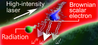
Figure 1: RR on a Brownian scalar electron. The signatures of $\omega$, $\omega^{\prime}$ and $\omega^{\prime\prime}$ denote sample paths of a scalar electron due to its randomness. By solving the Maxwell’s equation, RR in quantum dynamics is derived like in classical dynamics.

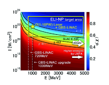
Figure 2: Quantumness of radiation, $q(\chi)$. This is the plot of Eq.(2) w.r.t. energies of an electron and laser intensities. When we choose the combination between a laser intensity of $O(10^{22}\mathrm{W}/\mathrm{cm}^{2})$ and an electron energy of $O(1\mathrm{GeV})$, the factor $q(\chi)$ reaches $0.3$ which is the feasible regime produced by the ELI-NP facility [1]. The SLAC E-144 included the experiments of the non-linear Compton scatterings by the combination of $O(10^{18}\mathrm{W}/\mathrm{cm}^{2}+46\mathrm{GeV})$ [16].

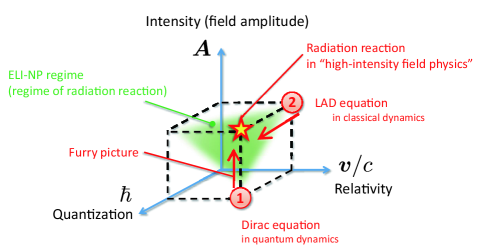
Figure 3: The physical regime of a scalar electron with RR. The point at “the star” is the regime of high-intensity field physics. The Furry picture is the first way from relativistic quantum dynamics to the point of “the star” where $q(\chi)$ is not unity. On the other hand, the quantization after reaching high-intensity “classical” dynamics is its second candidate.

For the second idea, we should refer classical RR model. RR has been treated by the Lorentz-Abraham-Dirac (LAD) equation as its standard model [22]:

$$m_{0}\frac{dv^{\mu}}{d\tau} =-e(F_{\mathrm{ex}}^{\mu\nu}+F_{\mathrm{LAD}}^{\mu\nu})v_{\nu}$$ (4)

$$F_{\mathrm{LAD}}^{\mu\nu}(x) =-\frac{m_{0}\tau_{0}}{ec^{2}}\left[\frac{d^{3}x^{\mu}}{d\tau^{3}}\cdot\frac{dx^{\nu}}{d\tau}-\frac{d^{3}x^{\nu}}{d\tau^{3}}\cdot\frac{dx^{\mu}}{d\tau}\right]$$ (5)

With the metric $g=(+,-,-,-)$ and $\tau_{0}\coloneqq e^{2}/6\pi\varepsilon_{0}m_{0}c^{3}$. The force $-eF_{\mathrm{LAD}}^{\mu\nu}v_{\nu}$ represents the interaction of RR acting on a scalar electron. When we can find the quantization of Eq.(4) with Eq.(5), it is not known how this affects Eq.(1), especially, $q(\chi)$ by any laser field profiles. We are then to study quantum dynamics of RR by adopting Nelson’s stochastic quantization [23, 24] as the second candidate in Fig.3, which can draw a real trajectory of a quanta by a Brownian motion. In addition, that achievement regarded as one of the few application of Nelson’s stochastic quantization.

However, its well-defined relativistic version and the Maxwell equation have been absent. Thus, we resolve the following issues for RR in this article. For $\{\hat{x}(\tau,\omega)\}_{\tau\in\mathbb{R}}$ a Brownian trajectory, $\langle\mathrm{A}\rangle$ the set of the relativistic Brownian kinematics and the dynamics for a scalar electron

$$d_{\pm}\hat{x}^{\mu}(\tau,\omega) =\mathcal{V}_{\pm}^{\mu}(\hat{x}(\tau,\omega))d\tau+\lambda\times dW_{\pm}^{\mu}(\tau,\omega)$$ (6)

$$m_{0}\mathfrak{D_{\tau}}\mathcal{V}^{\mu}(\hat{x}(\tau,\omega)) =-e\mathcal{\hat{V}}_{\nu}(\hat{x}(\tau,\omega))F^{\mu\nu}(\hat{x}(\tau,\omega))$$ (7)

is regarded as the Klein-Gordon (KG) equation with $\mathcal{V}^{\mu}(x)\coloneqq 1/m_{0}\times\left[i\hbar\partial{}^{\mu}\ln\phi(x)+eA{}^{\mu}(x)\right]$ given by its wave function $\phi$ and $\{W_{\pm}(\tau,\omega)\}_{\tau\in\mathbb{R}}$ of Wiener processes [Sect.3]. And also $\langle\mathrm{B}\rangle$ the Maxwell equation with a current of a Brownian scalar electron [Sect.4]

$$\partial_{\mu}[F^{\mu\nu}(x)+\delta f^{\mu\nu}(x)] =\mu_{0}\times\mathbb{E}\left\llbracket-ec\int_{\mathbb{R}}d\tau\,\mathrm{Re}\left\{\mathcal{V}^{\nu}(x)\right\}\delta^{4}(x-\hat{x}(\tau,\bullet))\right\rrbracket$$ (8)

is constructed. We propose $\langle\mathrm{C}\rangle$ an action integral to give the above Eq.(7) and Eq.(8) in this model, too [Sect.5]. In the fact, the consistent system of Eqs.(6-7) and Eq.(8) has been absent after Nelson’s first article [23]. Especially, the charge current in Eq.(8) adapting stochastic quantization has not been discovered for a long time. So, this is the first proposal for the coupling system between a relativistic Brownian quanta and fields. To describe its interaction is, therefore, a new result. Namely by solving Eq.(8) in Sect.6, we derive $\langle\mathrm{D}\rangle$ RR in quantum dynamics

$$m_{0}\mathfrak{D_{\tau}}\mathcal{V}^{\mu}(\hat{x}(\tau,\omega))) =-eF_{\mathrm{ex}}^{\mu\nu}(\hat{x}(\tau,\omega)\mathcal{V}_{\nu}(\hat{x}(\tau,\omega))-e\mathfrak{F}^{\mu\nu}(\hat{x}(\tau,\omega))\mathcal{V}_{\nu}(\hat{x}(\tau,\omega))$$ (9)

$$\mathfrak{F}^{\mu\nu}(\hat{x}(\tau,\omega)) =-\frac{m_{0}\tau_{0}}{ec^{2}}\int_{\varOmega_{(\tau,\omega)}}d\mathscr{P}(\omega^{\prime})\left[\begin{gathered}\dot{a}^{\mu}(\hat{x}(\tau,\omega^{\prime}))\cdot\mathrm{Re}\{\mathcal{V}^{\nu}(\hat{x}(\tau,\omega^{\prime}))\}\\ -\dot{a}^{\nu}(\hat{x}(\tau,\omega^{\prime}))\cdot\mathrm{Re}\{\mathcal{V}^{\mu}(\hat{x}(\tau,\omega^{\prime}))\}\end{gathered}\right]$$ (12)

with $\dot{a}^{\mu}(x)\approx\mathrm{Re}\{\mathfrak{D_{\tau}}^{2}\mathcal{V}^{\mu}(x)\}$, i.e., the quantization of the LAD equation (4-5). The readers can find the similarity between Eqs.(4-5) and Eqs.(9-12) by the comparison. In the fact, $\lim_{\hbar\rightarrow 0}\mathfrak{F}=F_{\mathrm{LAD}}$ is ensured. Thus, Eqs.(9-12) becomes Eqs.(4-5) in the classical limit. This easy comparison is the reason why we study stochastic quantization for RR. By its Ehrenfest’s theorem, $\langle\mathrm{E}\rangle$ a radiation formula

$$\frac{dW_{\mathrm{stochastic}}}{dt} =-m_{0}\tau_{0}\mathscr{P}(\varOmega_{\tau}^{\mathrm{ave}})\frac{d^{2}\langle\hat{x}_{\mu}\rangle_{\tau}}{d\tau^{2}}\cdot\frac{d^{2}\langle\hat{x}^{\mu}\rangle_{\tau}}{d\tau^{2}}$$ (13)

similar to Eq.(1) is imposed. This shows the fact that $q(\chi)$ is $\mathscr{P}(\varOmega_{\tau}^{\mathrm{ave}})$ a probability which a scalar electron stays at its average position. Finally, a possibility of its higher-order corrections is discussed.

Let us note a naive idea of quantum dynamics. The present proposal does not deny the previous formulations of quantum dynamics. As K. Yasue suggests [25], quantum dynamics is symbolically illustrated by

$$(\mathrm{Quantum\,dynamics}) =(\mathrm{Matrix\,mechanics})\cup(\mathrm{Wave\,mechanics})\cup(\mathrm{Path\,integral})$$

$$\quad\quad\cup(\mathrm{Stochastic\,quantization})\cup(\mathrm{Something\,else}).$$

So, each expressions of quantum dynamics are complementary via a wave function.

Before discussing the relativistic regime, let us summarize Nelson’s model in the non-relativistic regime by a 1D stochastic process (an (S3)-processes) in the following Sect.2.

2 Stochastic kinematics and dynamics in non-relativistic regime by a 1D stochastic process

2.1 Kinematics

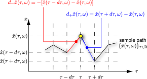
(A)

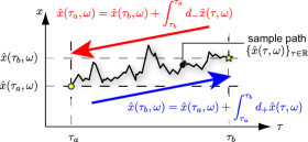
(B)

Figure 4: $d_{+}\hat{x}(\tau,\omega)$ and $d_{-}\hat{x}(\tau,\omega)$ of the fractions of a continuous stochastic process $\{\hat{x}(\tau,\omega)\}_{\tau\in\mathbb{R}}$. Let us draw a sample path $\{\hat{x}(\tau,\omega)\}_{\tau\in\mathbb{R}}$, then, consider how to generate this by stochastic differential equations. (A) Due to the non-differentiability of $\{\hat{x}(\tau,\omega)\}_{\tau\in\mathbb{R}}$, we have to define Eq.(16) as the two types of its evolution at $\hat{x}(\tau,\omega)$; $d_{+}\hat{x}(\tau,\omega)$ for a $\{\mathcal{P}_{\tau}\}$-prog. of a normal diffusion process, and $d_{-}\hat{x}(\tau,\omega)$ for an $\{\mathcal{F}_{\tau}\}$-prog. of an inverse process of a $\{\mathcal{P}_{\tau}\}$-prog. See also Fig.5 for this. (B) a curve $\{\hat{x}(\tau,\omega)\}_{\tau\in[\tau_{a},\tau_{b}]}$ is imposed by (A). For the initial value $\hat{x}(\tau_{a},\omega)$, $\hat{x}(\tau_{b},\omega)$ is found by a forward (normal) diffusion as a $\{\mathcal{P}_{\tau}\}$-prog., i.e., $\hat{x}(\tau_{b},\omega)=\hat{x}(\tau_{a},\omega)+\int_{\tau_{a}}^{\tau_{b}}d_{+}\hat{x}(\tau,\omega)$. On the other hand, an $\{\mathcal{F}_{\tau}\}$-prog. is regarded as a backward diffusion $\hat{x}(\tau_{a},\omega)=\hat{x}(\tau_{b},\omega)+\int_{\tau_{b}}^{\tau_{a}}d_{-}\hat{x}(\tau,\omega)$ with the terminal value $\hat{x}(\tau_{b},\omega)$. This is the reason why we have the two expressions of “$+$” and “$-$”.

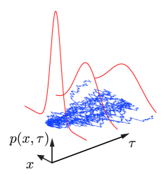
(a) $\partial_{\tau}p(x,\tau)=1/2\times\partial_{x}^{2}p(x,\tau)$

as a $\{\mathcal{P}_{\tau}\}$-WP

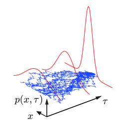
(b) $\partial_{\tau}p(x,\tau)=-1/2\times\partial_{x}^{2}p(x,\tau)$

as an $\{\mathcal{F}_{\tau}\}$-WP

Figure 5: Trajectories and probabilities of WPs. (a) a $\{\mathcal{P}_{\tau}\}$-WP and (b) an $\{\mathcal{F}_{\tau}\}$-WP. The blue lines are their sample paths and their probability densities are drawn by red.

For $\omega$ the label of sample paths, let $\{\hat{x}(\tau,\omega)\}_{\tau\in\mathbb{R}}$ a trajectory of a quanta with its existence probability of $\mathscr{P}^{1\mathrm{\mathchar 45\relax dim}}(\omega)$ be a 1D Nelson’s (S3)-process [24].

$$\hat{x}(\tau_{b},\omega)-\hat{x}(\tau_{a},\omega) =\int_{\tau_{a}}^{\tau_{b}}v_{\pm}(\hat{x}(\tau,\omega))d\tau+\lambda\times\int_{\tau_{a}}^{\tau_{b}}dw_{\pm}(\tau,\omega)$$ (14)

With $\lambda\coloneqq\sqrt{\hbar/m_{0}}$. Equation (14) is also written like

$$\hat{x}(\tau_{b},\omega)-\hat{x}(\tau_{a},\omega) =\int_{\tau_{a}}^{\tau_{b}}d_{\pm}\hat{x}(\tau,\omega)$$ (15)

by introducing its differential form

$$d_{\pm}\hat{x}(\tau,\omega) \coloneqq\pm[\hat{x}(\tau\pm d\tau,\omega)-\hat{x}(\tau,\omega)]$$

$$=v_{\pm}(\hat{x}(\tau,\omega))d\tau+\lambda\times dw_{\pm}(\tau,\omega).$$ (16)

This is a combination of a drift and its randomness governed by $\{w_{\pm}(\tau,\omega)\}_{\tau\in\mathbb{R}}$ of 1D Wiener processes (WP; or Brownian motion) such that

$$\mathbb{E}\llbracket dw_{\pm}(\tau,\bullet)\rrbracket= 0,$$ (17)

$$\mathbb{E}\llbracket[dw_{\pm}(\tau,\bullet)]^{2}\rrbracket= d\tau,$$ (18)

$$\mathbb{E}\llbracket dw_{+}(\tau,\bullet)\cdot dw_{-}(\tau,\bullet)\rrbracket= 0,$$ (19)

for $d\tau>0$. Where, $\mathbb{E}\llbracket f(\bullet)\rrbracket\coloneqq\int_{\varOmega}f(\omega)d\mathscr{P}^{1\mathrm{\mathchar 45\relax dim}}(\omega)$ the expectation of $\{f(\omega)\}_{\omega\in\varOmega}$. The two types of “$\pm$” are derived from the randomness of $\{\hat{x}(\tau,\omega)\}_{\tau\in\mathbb{R}}$, for the time reversibility; let “$\bm{\{\mathcal{P}_{\tau}\}}$-progressive (prog.)” denoted by “$+$” be a diffusion from $\tau_{a}$ to $\tau_{b}>\tau_{a}$. And “$\bm{\{\mathcal{F}_{\tau}\}}$-prog.” by “$-$” is an inverse process of “$\{\mathcal{P}_{\tau}\}$-prog.”  shown in Fig.4. Thus, an (S3)-process of Eqs.(14-16) is $\{\mathcal{P}_{\tau}\}$-prog. and $\{\mathcal{F}_{\tau}\}$-prog. “Progressive” means that a stochastic process $\{\hat{x}(\tau,\omega)\}_{(\tau,\omega)\in\mathbb{R}\times\varOmega}$ is integrable for $\tau$ and $\omega$, mathematically. For its probability density $p(x,\tau)\coloneqq d\mathscr{P}^{1\mathrm{\mathchar 45\relax dim}}/dx$, the difference between a $\{\mathcal{P}_{\tau}\}$-prog. and an $\{\mathcal{F}_{\tau}\}$-prog. appears in the forward ($+$) and backward ($-$) Fokker-Planck (FP) equations w.r.t. Eq.(16) [23, 24, 26],

$$\partial_{\tau}p(x,\tau)+\partial_{x}\left[v_{\pm}(x)p(x,\tau)\right]=\pm\frac{\lambda^{2}}{2}\partial_{x}^{2}p(x,\tau).$$ (20)

Figure 5 shows the difference between $\{\mathcal{P}_{\tau}\}$ and $\{\mathcal{F}_{\tau}\}$-WPs by their trajectories (the blue lines) and probabilities (the red lines) when $v_{\pm}=0$ in Eq.(20): (a) a $\{\mathcal{P}_{\tau}\}$-WP of a forward diffusion and (b) an $\{\mathcal{F}_{\tau}\}$-WP of a backward diffusion. Equation (20) is derived by the following Itô formula for $\{\hat{x}(\tau,\omega)\}_{\tau\in\mathbb{R}}$ of a $\{\mathcal{P}_{\tau}\}$-prog. and an $\{\mathcal{F}_{\tau}\}$-prog., respectively [27, 28]:

$$d_{\pm}f(\hat{x}(\tau,\omega)) =f^{\prime}(\hat{x}(\tau,\omega))\cdot d_{\pm}\hat{x}(\tau,\omega)\pm\frac{\lambda^{2}}{2}f^{\prime\prime}(\hat{x}(\tau,\omega))d\tau\,\,\,\,\mathrm{a.s.}$$ (21)

2.2 Dynamics

What Nelson performed after the above construction of the kinematics was the derivation of the Schrödinger equation $[i\hbar\partial_{t}+e\phi(x,t)]\psi(x,t)=-\hbar^{2}/2m_{0}\times\partial_{x}^{2}\psi(x,t)$ by the following with the field $E(x,t)\coloneqq-\partial_{x}\phi(x,t)$:

$$m_{0}\left[\begin{gathered}\partial_{t}v(x,t)+v(x,t)\cdot\partial_{x}v(x,t)-u(x,t)\cdot\partial_{x}u(x,t)-\frac{\hbar}{2m_{0}}\partial_{x}^{2}u(x,t)\end{gathered}\right] =-eE(x,t)$$ (23)

$$V(x,t) \coloneqq-i\frac{\hbar}{m_{0}}\partial_{x}\ln\psi(x,t)$$ (24)

$$v(x,t) =\mathrm{Re}\left\{V(x,t)\right\}$$ (25)

$$u(x,t) =-\mathrm{Im}\left\{V(x,t)\right\}$$ (26)

Where, $v\coloneqq(v_{+}+v_{-})/2$ and $u\coloneqq(v_{+}-v_{-})/2$ [23, 24]. By $V\coloneqq v-iu$, its compact form [29] appears:

$$m_{0}D_{t}V(x,t) =-eE(x,t)$$ (27)

$$D_{t} \coloneqq\partial_{t}+V(x,t)\partial_{x}-i\frac{\lambda}{2}\partial_{x}^{2}$$ (28)

Equation (27) is similar to $m_{0}dv/dt=-eE$ in classical dynamics. Then, $v_{+}$ and $v_{-}$ are reproduced by $V$ for Eqs.(14-16). Since this is coupled with Eq.(20), he succeeded to demonstrate the question why $\psi^{*}(x,t)\psi(x,t)$ is regarded as $p(x,t)$.

3 Stochastic kinematics and dynamics of a scalar electron by a 4D stochastic process

We give the set of the stochastic kinematics and dynamics of a scalar electron in this section, i.e, the quantization of $dx^{\mu}=v^{\mu}d\tau$ and $m_{0}dv^{\mu}=-ev_{\nu}F^{\mu\nu}$. It is recommended to read from Sect.3.4 to the readers who want to check its scheme briefly at first.

3.1 Kinematics

The following is a natural idea for a scalar electron in the 4D spacetime: We assume an expansion of Eq.(16) to the relativistic kinematics such that

$$d_{\pm}\hat{x}^{\mu}(\tau,\omega)=\mathcal{V}_{\pm}^{\mu}(\hat{x}(\tau,\omega))d\tau+\lambda\times dW_{\pm}^{\mu}(\tau,\omega)$$ (29)

for $\lambda\coloneqq\sqrt{\hbar/m_{0}}$ and $\mu=0,1,2,3$ with its existence probability $\mathscr{P}(\omega)$. It is coupled with $m_{0}\mathfrak{D_{\tau}}\mathcal{V}^{\mu}=-e\mathcal{\hat{V}}_{\nu}F^{\mu\nu}$ equivalent to the KG equation (see it later). As a mimic of the 1D case, we want to require the relativistic FP equation

$$\partial_{\tau}p(x,\tau)+\partial_{\mu}[\mathcal{V}_{\pm}^{\mu}(x)p(x,\tau)]=\mp\frac{\lambda^{2}}{2}\partial_{\mu}\partial^{\mu}p(x,\tau)$$ (30)

w.r.t. $p(x,\tau)\coloneqq d\mathscr{P}/d^{4}x$ and the Itô formula,

$$d_{\pm}f(\hat{x}(\tau,\omega)) =\partial_{\mu}f(\hat{x}(\tau,\omega))\cdot d_{\pm}\hat{x}^{\mu}(\tau,\omega)\pm\frac{\lambda^{2}}{2}(-g^{\mu\nu})\partial_{\mu}\partial_{\nu}f(\hat{x}(\tau,\omega))d\tau\,\,\,\,\mathrm{a.s.}$$ (31)

We will demonstrate the validity of the above adapting the KG equation well in the later discussion.

Anyway for $\{\hat{x}(\tau,\omega)\}_{\tau\in\mathbb{R}}$ of a 4D $\{\mathcal{P}_{\tau}\}$-prog., it imposes the expanded formula of Eq.(21); $d_{+}f(\hat{x}(\tau,\omega))=\partial_{\mu}f(\hat{x}(\tau,\omega))\cdot d_{+}\hat{x}^{\mu}(\tau,\omega)+\lambda^{2}/2\times\delta^{\mu\nu}\partial_{\mu}\partial_{\nu}f(\hat{x}(\tau,\omega))d\tau$ a.s. By comparing it with Eq.(31), $\delta^{\mu\nu}\partial_{\mu}\partial_{\nu}f(\hat{x}(\tau,\omega))$ has to be $(-g^{\mu\nu})\partial_{\mu}\partial_{\nu}f(\hat{x}(\tau,\omega))$. Therefore, let us introduce a $\{\mathscr{P}_{\tau}\}$-prog.  for “$+$” in Eq.(29)

$$\underset{\{\mathscr{P}_{\tau}\}\mathchar 45\relax\mathrm{prog.}}{\underbrace{\hat{x}(\tau,\omega)}}\coloneqq(\underset{\{\mathcal{F}_{\tau}\}\mathchar 45\relax\mathrm{prog.}}{\underbrace{\hat{x}^{0}(\tau,\omega)},}\underset{\{\mathcal{P}_{\tau}\}\mathchar 45\relax\mathrm{prog.}}{\underbrace{\hat{x}^{1}(\tau,\omega),\hat{x}^{2}(\tau,\omega),\hat{x}^{3}(\tau,\omega)}})$$

and an $\{\mathscr{F}_{\tau}\}$-prog. by “$-$”

$$\underset{\{\mathscr{F}_{\tau}\}\mathchar 45\relax\mathrm{prog.}}{\underbrace{\hat{x}(\tau,\omega)}}\coloneqq(\underset{\{\mathcal{P}_{\tau}\}\mathchar 45\relax\mathrm{prog.}}{\underbrace{\hat{x}^{0}(\tau,\omega)},}\underset{\{\mathcal{F}_{\tau}\}\mathchar 45\relax\mathrm{prog.}}{\underbrace{\hat{x}^{1}(\tau,\omega),\hat{x}^{2}(\tau,\omega),\hat{x}^{3}(\tau,\omega)}}).$$

Where, let $\{W_{+}(\tau,\omega)\}_{\tau\in\mathbb{R}}$ and $\{W_{-}(\tau,\omega)\}_{\tau\in\mathbb{R}}$ of WPs in Eq.(29) be $\{\mathscr{P}_{\tau}\}$ and $\{\mathscr{F}_{\tau}\}$-prog., respectively. Hereby, we name $\{\hat{x}(\tau,\omega)\}_{\tau\in\mathbb{R}}$ of a $\{\mathscr{P}_{\tau}\}$ and $\{\mathscr{F}_{\tau}\}$-prog. “a D-prog.” For $d\tau\geq 0$ and $\mathbb{E}\llbracket f(\bullet)\rrbracket\coloneqq\allowbreak\int_{\varOmega}f(\omega)\allowbreak d\mathscr{P}(\omega)$, the following rules are satisfied as the expansion of the 1D case:

$$\mathbb{E}\llbracket dW_{\pm}^{\mu}(\tau,\bullet)\rrbracket= 0$$ (32)

$$\mathbb{E}\llbracket dW_{\pm}^{\mu}(\tau,\bullet)\cdot dW_{\pm}^{\nu}(\tau,\bullet)\rrbracket=\delta^{\mu\nu}\times d\tau$$ (33)

$$\mathbb{E}\llbracket dW_{\pm}^{\mu}(\tau,\bullet)\cdot dW_{\mp}^{\nu}(\tau,\bullet)\rrbracket= 0$$ (34)

The definition of $d_{-}f(\hat{x}(\tau,\omega))$ by Eq.(31) can be checked by the expansion for an $\{\hat{x}(\tau,\omega)\}_{\tau\in\mathbb{R}}$ of $\{\mathscr{F}_{\tau}\}$-prog.,

$$d_{-}f(\hat{x}(\tau,\omega)) =f(\underset{\{\mathcal{P}_{\tau}\}\mathchar 45\relax\mathrm{\mathrm{prog.}}}{\underbrace{\hat{x}^{0}(\tau+d\tau,\omega)},}\underset{\{\mathcal{F}_{\tau}\}\mathchar 45\relax\mathrm{\mathrm{prog.}}}{\underbrace{\hat{x}^{i=1,2,3}(\tau,\omega)}})-f(\hat{x}^{0}(\tau,\omega),\hat{x}^{i=1,2,3}(\tau-d\tau,\omega))$$ (35)

with the help by Eq.(29) (a 4D version of Eq.(16) )

$$d_{-}\hat{x}(\tau,\omega) =(\underset{\{\mathcal{P}_{\tau}\}\mathchar 45\relax\mathrm{\mathrm{prog.}}}{\underbrace{\hat{x}^{0}(\tau+d\tau,\omega)},}\underset{\{\mathcal{F}_{\tau}\}\mathchar 45\relax\mathrm{\mathrm{prog.}}}{\underbrace{\hat{x}^{i=1,2,3}(\tau,\omega)}})-(\hat{x}^{0}(\tau,\omega),\hat{x}^{i=1,2,3}(\tau-d\tau,\omega))$$ (36)

to first order of $d\tau$. $d_{+}f(\hat{x}(\tau,\omega))$ is imposed by $\{\hat{x}(\tau,\omega)\}_{\tau\in\mathbb{R}}$ of a $\{\mathscr{P}_{\tau}\}$-prog. Let Eq.(31) be the general definition of $d_{\pm}$. The probability $\mathscr{P}(\omega)$ is calculated by the FP equation (30) since $p(x,\tau)\coloneqq d\mathscr{P}/d^{4}x$. Nelson introduced the drift velocities via the so-called mean derivatives [23]. In the present case, it is evaluated by

$$\mathcal{V}_{\pm}^{\mu}(\hat{x}(\tau,\omega))\coloneqq\mathbb{E}\left\llbracket\left.\frac{d_{\pm}\hat{x}^{\mu}}{d\tau}(\tau,\bullet)\right|\hat{x}(\tau,\omega)\right\rrbracket(\omega).$$ (37)

Where, $\mathbb{E}\llbracket f(\hat{x}(\tau,\bullet))|\mathscr{C}\rrbracket(\omega)=\int f(\hat{x}(\tau,\omega))d\mathscr{P}_{\mathscr{C}}(\omega)$ the conditional expectation for $\mathscr{P}_{\mathscr{C}}(X)$ a conditional probability of $X$ given $\mathscr{C}$.

Then, we define the complex differential $\hat{d}\coloneqq(d_{+}+d_{-})/2-i(d_{+}-d_{-})/2$ symbolically such that

$$\hat{d}f(\hat{x}(\tau,\omega)) =\partial_{\mu}f(\hat{x}(\tau,\omega))\cdot\hat{d}\hat{x}^{\mu}(\tau,\omega)-\frac{i\lambda^{2}}{2}\partial_{\mu}\partial^{\mu}f(\hat{x}(\tau,\omega))d\tau\,\,\,\,\mathrm{a.s.}$$ (38)

and the complex velocity

$$\mathcal{V}^{\mu}(\hat{x}(\tau,\omega)) \coloneqq\mathbb{E}\left\llbracket\left.\frac{\hat{d}\hat{x}^{\mu}}{d\tau}(\tau,\bullet)\right|\hat{x}(\tau,\omega)\right\rrbracket(\omega)$$ (39)

$$=\frac{\mathcal{V}_{+}^{\mu}(\hat{x}(\tau,\omega))+\mathcal{V}_{-}^{\mu}(\hat{x}(\tau,\omega))}{2}-i\frac{\mathcal{V}_{+}^{\mu}(\hat{x}(\tau,\omega))-\mathcal{V}_{-}^{\mu}(\hat{x}(\tau,\omega))}{2}$$

with its other assumption [29]:

$$\mathcal{V}^{\mu}(x)\coloneqq\frac{1}{m_{0}}\times\left[i\hbar\partial{}^{\mu}\ln\phi(x)+eA{}^{\mu}(x)\right]$$ (40)

Let $||A||_{(g,\mathbb{C}^{4})}^{2}\coloneqq A_{\mu}^{*}A^{\mu}$ ($A^{*}$ is the complex conjugate of a vector $A$) on the Minkowski spacetime,

$$d\tau\coloneqq\frac{1}{c}\times\sqrt{\mathbb{E}\left\llbracket||\hat{d}\hat{x}(\tau,\bullet)-\lambda\times\hat{d}W(\tau,\bullet)||_{(g,\mathbb{C}^{4})}^{2}\right\rrbracket}$$ (41)

of the proper time links to the Lorentz invariant

$$\mathbb{E}\left\llbracket\mathcal{V}_{\mu}^{*}(\hat{x}(\tau,\bullet))\mathcal{V}^{\mu}(\hat{x}(\tau,\bullet))\right\rrbracket=c^{2}\,.$$ (42)

For satisfying Eq.(42), $\phi$ in Eq.(40) has to be a wave function of the KG equation with $i\hbar\mathfrak{D}_{\alpha}\coloneqq i\hbar\partial_{\alpha}+eA_{\alpha}(x)$,

$$(i\hbar\mathfrak{D}_{\alpha})\cdot(i\hbar\mathfrak{D}^{\alpha})\phi(x)-m_{0}^{2}c^{2}\phi(x)=0$$ (43)

as Ref.[30] suggests. Namely by

$$\mathcal{V}_{\mu}^{*}(x)\mathcal{V}^{\mu}(x) =\frac{1}{m_{0}^{2}}\times\frac{\mathrm{Re}\{\phi^{*}(x)(i\hbar\mathfrak{D}_{\mu})\cdot(i\hbar\mathfrak{D}^{\mu})\phi(x)\}}{\phi^{*}(x)\phi(x)}+\frac{\hbar^{2}}{2m_{0}^{2}}\times\frac{\partial_{\mu}\partial^{\mu}[\phi(x)\cdot\phi^{*}(x)]}{\phi^{*}(x)\phi(x)},$$ (44)

the first term in RHS is $c^{2}$ and the second term becomes zero by its expectation after the substitution $x=\hat{x}(\tau,\omega)$. Let us demonstrate this in the end of the next small section for the probability density.

3.2 Equations of probability density

By using this complex velocity, the FP equation of Eq.(30) derives the equation of continuity for $p$, w.r.t. $x\in\hat{x}(\tau,\varOmega)\coloneqq\{\hat{x}(\tau,\omega)\}_{\omega\in\varOmega}$.

$$\partial_{\tau}p(x,\tau)+\partial_{\mu}\left[\mathrm{Re}\{\mathcal{V}^{\mu}(x)\}p(x,\tau)\right]=0$$ (45)

Then for a naturally boundary condition $p(x,\pm\infty)=0$,

$$\partial_{\mu}\left[\mathrm{Re}\{\mathcal{V}^{\mu}(x)\}\int_{\mathbb{R}}d\tau\,p(x,\tau)\right]=0$$ (46)

is found. Or by using

$$p(x,\tau)\coloneqq\mathbb{E}\llbracket\delta^{4}(x-\hat{x}(\tau,\bullet))\rrbracket$$ (47)

due to the definition of $\mathbb{E}\llbracket f(\hat{x}(\tau,\bullet))\rrbracket$, i.e.,

$$\mathbb{E}\llbracket f(\hat{x}(\tau,\bullet))\rrbracket \coloneqq\int_{\varOmega}f(\hat{x}(\tau,\omega^{\prime})))d\mathscr{P}(\omega^{\prime})$$ (48)

$$=\int_{\mathbb{R}^{4}}f(x^{\prime})p(x^{\prime},\tau)d^{4}x^{\prime},$$ (49)

the following is imposed:

$$\partial_{\mu}\mathbb{E}\left\llbracket-ec\int_{\mathbb{R}}d\tau\,\mathrm{Re}\{\mathcal{V}^{\mu}(x)\}\delta^{4}(x-\hat{x}(\tau,\bullet))\right\rrbracket=0$$ (50)

This is the conservation law of the current density

$$j_{\mathrm{stochastic}}^{\mu}(x)\coloneqq\mathbb{E}\left\llbracket-ec\int_{\mathbb{R}}d\tau\,\mathrm{Re}\left\{\mathcal{V}^{\mu}(x)\right\}\delta^{4}(x-\hat{x}(\tau,\bullet))\right\rrbracket$$ (51)

in the 4D spacetime (see this role in Sect.4). The following relation is also found by Eq.(30).

$$\mathrm{Im}\{\mathcal{V}^{\mu}(x)\} =\begin{cases}\begin{gathered}\frac{\lambda^{2}}{2}\times\partial^{\mu}\ln p(x,\tau)\end{gathered},&\begin{gathered}x\in\hat{x}(\tau,\varOmega)\end{gathered}\\ \begin{gathered}\frac{\lambda^{2}}{2}\times\partial^{\mu}\ln\int_{\mathbb{R}}d\tau\,p(x,\tau)\end{gathered},&x\in\bigcup_{\tau\in\mathbb{R}}\hat{x}(\tau,\varOmega)\end{cases}$$ (52)

Where, $\bigcup_{\tau\in\mathbb{R}}\hat{x}(\tau,\varOmega)=\mathrm{supp}(\int_{\mathbb{R}}d\tau\,p(\circ,\tau))$. Equation (52) is a mimic of the osmotic pressure formula [23, 24].

Let us come back to the discussion of Eq.(42) and Eq.(44) (see also [30]). By $\phi(x)\coloneqq\exp[R(x)/\hbar+iS(x)/\hbar]$ w.r.t. $R$ and $S$ of real-valued functions, $\phi^{*}(x)\phi(x)=\exp[2R(x)/\hbar]$. Where, $\partial^{\mu}R(x)=\mathrm{Im}\{m_{0}\mathcal{V}^{\mu}(x)\}=\hbar/2\times\partial^{\mu}\ln p(x,\tau)$ by Eq.(40) and Eq.(52) for $x\in\hat{x}(\tau,\varOmega)$. Thus,

$$\frac{\hbar^{2}}{2m_{0}^{2}}\times\frac{\partial_{\mu}\partial^{\mu}[\phi(x)\cdot\phi^{*}(x)]}{\phi^{*}(x)\phi(x)}= \frac{\hbar^{2}}{2m_{0}^{2}}\times\frac{\partial_{\mu}\partial^{\mu}p(x,\tau)}{p(x,\tau)}.$$ (53)

After assuming $\phi$ as the solution of the KG equation (43),

$$\mathbb{E}\llbracket\mathcal{V}_{\mu}^{*}(\hat{x}(\tau,\bullet))\mathcal{V}^{\mu}(\hat{x}(\tau,\bullet))\rrbracket =c^{2}+\frac{\hbar^{2}}{2m_{0}^{2}}\times\mathbb{E}\left\llbracket\frac{\partial_{\mu}\partial^{\mu}p(\hat{x}(\tau,\bullet),\tau)}{p(\hat{x}(\tau,\bullet),\tau)}\right\rrbracket$$

$$=c^{2}+\frac{\hbar^{2}}{2m_{0}^{2}}\times\int_{\mathbb{R}^{4}}d^{4}x\,\partial_{\mu}\partial^{\mu}p(x,\tau),$$ (54)

Eq.(42) is found by $\partial^{\mu}p(x,\tau)|_{x\in\partial\mathbb{R}^{4}}=0$ the boundary condition on $\partial\mathbb{R}^{4}$ the boundary of $\mathbb{R}^{4}$.

3.3 Dynamics

Let us give the equation of Nottale’s style [29] for the dynamics of a Brownian scalar electron:

$$m_{0}\mathfrak{D_{\tau}}\mathcal{V}^{\mu}(\hat{x}(\tau,\omega))=-e\mathcal{\hat{V}}_{\nu}(\hat{x}(\tau,\omega))F^{\mu\nu}(\hat{x}(\tau,\omega))$$ (55)

$$\hat{\mathcal{V}}^{\mu}(x) \coloneqq\mathcal{V}^{\mu}(x)+i\frac{\lambda^{2}}{2}\times\partial^{\mu}$$ (56)

$$\mathfrak{D_{\tau}} \coloneqq\hat{\mathcal{V}}^{\mu}(x)\cdot\partial_{\mu}$$ (57)

Equations (55-57) corresponds to $m_{0}dv^{\mu}/dt=-ev_{\nu}F^{\mu\nu}$ in classical dynamics and it implies the KG equation [29] since

$$\mathfrak{D_{\tau}}\mathcal{V}^{\mu}+\frac{e}{m_{0}}\mathcal{\hat{V}}_{\nu}F^{\mu\nu} =\begin{gathered}\frac{1}{2}\partial^{\mu}\left[\frac{(i\hbar\partial_{\nu}+eA_{\nu})(i\hbar\partial^{\nu}+eA{}^{\nu})\phi}{m_{0}^{2}\phi}\right]\end{gathered}$$ (59)

$$=0.$$ (60)

We can easily clarify that Eq.(55) satisfies the $U(1)$-gauge symmetry. Let us study the relation between Eq.(42) and Eq.(55). This relation corresponds to the one between $v_{\mu}v^{\mu}=c^{2}$ and $d/d\tau(v_{\mu}v^{\mu})=0$ in classical dynamics. The readers may find another definition of $\mathfrak{D_{\tau}}$:

$$\mathfrak{D}_{\tau}^{\pm}\coloneqq\mathbb{E}\left\llbracket\left.\frac{d_{\pm}}{d\tau}\right|\hat{x}(\tau,\omega)\right\rrbracket$$ (61)

$$\mathfrak{D}_{\tau}\coloneqq\mathbb{E}\left\llbracket\left.\frac{\hat{d}}{d\tau}\right|\hat{x}(\tau,\omega)\right\rrbracket=\frac{1-i}{2}\mathfrak{D}_{\tau}^{+}+\frac{1+i}{2}\mathfrak{D}_{\tau}^{-}$$ (62)

Nelson introduced the partial integral formula for his (S3)-process. In our case for $\{\hat{x}(\tau,\omega)\}$ of a D-prog., the differential form of that formula for $\{\alpha^{\mu}\}_{\mu=0,1,2,3}$ and $\{\beta^{\mu}\}_{\mu=0,1,2,3}$ of complex functions is

$$\frac{d}{d\tau}\mathbb{E}\llbracket\alpha_{\mu}(\hat{x}(\tau,\bullet))\beta^{\mu}(\hat{x}(\tau,\bullet))\rrbracket =\mathbb{E}\left\llbracket\mathfrak{D}_{\tau}^{\pm}\alpha_{\mu}(\hat{x}(\tau,\bullet))\cdot\beta^{\mu}(\hat{x}(\tau,\bullet))+\alpha_{\mu}(\hat{x}(\tau,\bullet))\cdot\mathfrak{D}_{\tau}^{\mp}\beta^{\mu}(\hat{x}(\tau,\bullet))\right\rrbracket.$$ (63)

By linear combining the above “$+$” and “$-$” formulas,

$$\frac{d}{d\tau}\mathbb{E}\llbracket\alpha_{\mu}(\hat{x}(\tau,\bullet))\beta^{\mu}(\hat{x}(\tau,\bullet))\rrbracket =\mathbb{E}\left\llbracket\mathfrak{D}_{\tau}\alpha_{\mu}(\hat{x}(\tau,\bullet))\cdot\beta^{\mu}(\hat{x}(\tau,\bullet))+\alpha_{\mu}(\hat{x}(\tau,\bullet))\cdot\mathfrak{D}_{\tau}^{*}\beta^{\mu}(\hat{x}(\tau,\bullet))\right\rrbracket$$ (64)

$$=\mathbb{E}\left\llbracket\mathfrak{D}_{\tau}^{*}\alpha_{\mu}(\hat{x}(\tau,\bullet))\cdot\beta^{\mu}(\hat{x}(\tau,\bullet))+\alpha_{\mu}(\hat{x}(\tau,\bullet))\cdot\mathfrak{D}_{\tau}\beta^{\mu}(\hat{x}(\tau,\bullet))\right\rrbracket.$$ (65)

When $\alpha_{\mu}=\mathcal{V}_{\mu}^{*}$ and $\beta^{\mu}=\mathcal{V}^{\mu}$ in Eq.(65),

$$\frac{d}{d\tau}\mathbb{E}\left\llbracket\mathcal{V}_{\mu}^{*}(\hat{x}(\tau,\bullet))\mathcal{V}^{\mu}(\hat{x}(\tau,\bullet))\right\rrbracket =\mathbb{E}\left\llbracket\mathcal{V}_{\mu}^{*}(\hat{x}(\tau,\bullet))\cdot\mathfrak{D_{\tau}}\mathcal{V}^{\mu}(\hat{x}(\tau,\bullet))+\mathfrak{D_{\tau}}^{*}\mathcal{V}_{\mu}^{*}(\hat{x}(\tau,\bullet))\cdot\mathcal{V}^{\mu}(\hat{x}(\tau,\bullet))\right\rrbracket$$

$$=\frac{\lambda^{4}e}{2m_{0}}\times\int_{\mathbb{R}^{4}}d^{4}x\,p(x,\tau)\cdot\partial_{\mu}\partial_{\nu}F^{\mu\nu}(x)$$

$$=0$$ (66)

is found. Thus, Eq.(42) is supported by Eq.(55) the dynamics of a Brownian quanta, too.

Consider the expectation of Eq.(55), Ehrenfest’s theorem is imposed naturally for $\langle\hat{x}\rangle_{\tau}\coloneqq\mathbb{E}\llbracket\hat{x}(\tau,\bullet)\rrbracket$ and $\delta\hat{x}(\tau,\omega)\coloneqq\hat{x}(\tau,\omega)-\langle\hat{x}\rangle_{\tau}$:

$$m_{0}\frac{d^{2}\langle\hat{x}^{\mu}\rangle_{\tau}}{d\tau^{2}} =\mathbb{E}\left\llbracket-eF^{\mu\nu}(\hat{x}(\tau,\bullet))\mathrm{Re}\{\mathcal{V}_{\nu}(\hat{x}(\tau,\bullet))\}\right\rrbracket$$ (67)

$$=-eF^{\mu\nu}(\langle\hat{x}\rangle_{\tau})\frac{d\langle\hat{x}_{\nu}\rangle_{\tau^{\prime}}}{d\tau}+O(\langle\otimes^{2}\delta\hat{x}\rangle_{\tau})$$ (68)

$d\langle\hat{x}\rangle_{\tau}/d\tau-\mathrm{Re}\{\mathcal{V}(\langle\hat{x}\rangle_{\tau})\}=O(\langle\otimes^{2}\delta\hat{x}\rangle_{\tau})$ is employed since $d\langle\hat{x}\rangle_{\tau}/d\tau=\mathbb{E}\llbracket\mathrm{Re}\{\mathcal{V}(\hat{x}(\tau,\bullet)\}\rrbracket$ by Eqs.(64,65) for $\alpha^{\mu}(x)=x^{\mu}$ and $\beta^{\mu}(x)=1$. Hereby, the requirement of the issue-$\langle\mathrm{A}\rangle$, the system of relativistic kinematics and dynamics of a scalar electron is completed.

3.4 Schematic method of stochastic quantization

For obtaining Eq.(55) the equations of quantum dynamics of a relativistic quanta from classical dynamics, let us conclude the above discussion schematically. At first, we regard classical dynamics as the combination of the kinematics

$$dx^{\mu}(\tau) =v^{\mu}(\tau)d\tau$$ (69)

and its dynamics

$$m_{0}\frac{dv^{\mu}}{d\tau} =-ev_{\nu}(\tau)F^{\mu\nu}(x(\tau)).$$ (70)

By considering that this kinematics is deduced from the expectation of Eq.(29), namely, $\mathbb{E}\llbracket d_{\pm}\hat{x}^{\mu}(\tau,\bullet)\rrbracket=v^{\mu}(\tau)d\tau$, the above classical dynamics is considered as the one by Ehrenfest’s theorem. Hence, the classical kinematics and dynamics are replaced by

$$\mathbb{E}\llbracket d_{\pm}\hat{x}^{\mu}(\tau,\bullet)\rrbracket =\frac{d\langle\hat{x}\rangle_{\tau}}{d\tau}d\tau,$$ (71)

$$m_{0}\frac{d^{2}\langle\hat{x}^{\mu}\rangle_{\tau}}{d\tau^{2}}=\mathbb{E}\left\llbracket-e\mathrm{Re}\{\mathcal{V}_{\nu}(\hat{x}(\tau,\bullet))\}F^{\mu\nu}(\hat{x}(\tau,\bullet))\right\rrbracket.$$ (72)

Since $d^{2}\langle\hat{x}^{\mu}\rangle_{\tau}/d\tau^{2}=\mathbb{E}\llbracket\mathrm{Re}\{\mathfrak{D_{\tau}}\mathcal{V}(\hat{x}(\tau,\bullet)\}\rrbracket$, Eq.(55) the dynamics of a Brownian scalar electron is found with its complex conjugate. This is the schematic method of stochastic quantization.

4 Maxwell equation

The Maxwell equation (the issue-$\langle\mathrm{B}\rangle$) is also given by

$$\partial_{\mu}[F^{\mu\nu}(x)+\delta f^{\mu\nu}(x)] =\mu_{0}\times\mathbb{E}\left\llbracket-ec\int_{\mathbb{R}}d\tau^{\prime}\mathrm{Re}\left\{\mathcal{V}^{\nu}(x)\right\}\delta^{4}(x-\hat{x}(\tau^{\prime},\bullet))\right\rrbracket$$ (73)

corresponding to

$$\partial_{\mu}[F^{\mu\nu}(x)+\delta f^{\mu\nu}(x)] =\mu_{0}\times\left[-ec\int_{\mathbb{R}}d\tau^{\prime}\frac{dx^{\nu}}{d\tau}(\tau^{\prime})\times\delta^{4}(x-x(\tau^{\prime}))\right]$$ (74)

in classical physics. Where, we will use $\delta f$ as a singular field attached to a quanta like the Coulomb field. $j_{\mathrm{stochastic}}$ of the current density given by Eq.(51) (and in Eq.(73)) is equal to one of a KG particle, i.e., $j_{\mathrm{stochastic}}=j_{\mathrm{\mathrm{K\mathchar 45\relax G}}}$,

$$j_{\mathrm{\mathrm{K\mathchar 45\relax G}}}^{\mu}(x)=-\frac{iec\lambda^{2}}{2}\left[\phi^{*}(x)\mathfrak{D}^{\mu}\phi(x)-\phi(x)(\mathfrak{D}^{*})^{\mu}\phi^{*}(x)\right]$$ (75)

by the assumption

$$\phi^{*}(x)\phi(x)=\int_{\mathbb{R}}d\tau^{\prime}p(x,\tau^{\prime}).$$ (76)

Since $\partial_{\mu}j_{\mathrm{stochastic}}^{\mu}(x)=0$, $\partial_{\mu}j_{\mathrm{\mathrm{K\mathchar 45\relax G}}}^{\mu}(x)=0$ and

$$j_{\mathrm{stochastic}}^{\mu}(x)= \frac{\int_{\mathbb{R}}d\tau^{\prime}p(x,\tau^{\prime})}{\phi^{*}(x)\phi(x)}\times j_{\mathrm{\mathrm{K\mathchar 45\relax G}}}^{\mu}(x),$$ (77)

therefore, $\partial_{\mu}[\int_{\mathbb{R}}d\tau^{\prime}p(x,\tau^{\prime})/\phi^{*}(x)\phi(x)]=0$ has to be satisfied. We emphasize that Eq.(76) is considered as the normalization of $\phi$ a wave function of the KG equation corresponding to one of the Schrödinger equation. The quantum effect of RR appearing in Eq.(1) is derived by the definition of $j_{\mathrm{stochastic}}^{\mu}$ obviously. When we write it such as

$$j_{\mathrm{stochastic}}^{\mu}(x) =-ec\int_{\mathbb{R}}d\tau^{\prime}\int_{\omega^{\prime}\in\varOmega}d\mathscr{P}(\omega^{\prime})\mathrm{Re}\left\{\mathcal{V}^{\mu}(x)\right\}\delta^{4}(x-\hat{x}(\tau^{\prime},\omega^{\prime})),$$ (78)

its classical limit ($\hbar\rightarrow 0$) converge to a path $\omega_{0}$ a smooth trajectory of $\{x(\tau)\}_{\tau\in\mathbb{R}}\coloneqq\{\hat{x}(\tau,\omega_{0})\}_{\tau\in\mathbb{R}}$. Then, Eq.(74) is deduced from Eq.(73), namely,

$$\lim_{\hbar\rightarrow 0}j_{\mathrm{stochastic}}^{\mu}(x) =-ec\int_{\mathbb{R}}d\tau^{\prime}\frac{dx^{\mu}}{d\tau}(\tau^{\prime})\delta^{4}(x-x(\tau^{\prime})).$$ (79)

See Sect.6.2 for more detail of the classical limit. In Ref.[15],

$$j_{\mathrm{Ref.}\cite[cite]{[\@@bibref{}{Seto(2015)}{}{}]}}^{\mu}(x) =-ec\int_{\mathbb{R}}d\tau^{\prime}q(\chi(\tau^{\prime}))\frac{dx^{\mu}}{d\tau}(\tau^{\prime})\delta^{4}(x-x(\tau^{\prime}))$$ (80)

is introduced for the QED correction. We can assume that $q(\chi)$ is associated by the probability measure of $\mathscr{P}$ by the comparison between Eq.(78) and Eq.(80).

5 Action integral

Let us give the systematic way to define Eq.(55) and Eq.(73) by the following action integral (issue-$\langle\mathrm{C}\rangle$):

$$\mathfrak{S}_{0}[\hat{x},A] =\int_{\mathbb{R}}d\tau\mathbb{E}\left\llbracket\frac{m_{0}}{2}\mathcal{V}_{\alpha}^{*}(\hat{x}(\tau,\bullet))\mathcal{V}^{\alpha}(\hat{x}(\tau,\bullet))\right\rrbracket$$

$$\quad\quad+\int_{\mathbb{R}}d\tau\mathbb{E}\left\llbracket-eA_{\alpha}(\hat{x}(\tau,\bullet))\mathrm{Re}\{\mathcal{V}^{\alpha}(\hat{x}(\tau,\bullet))\}\right\rrbracket$$

$$\quad\quad\quad+\int_{\mathbb{R}^{4}}d^{4}x\frac{1}{4\mu_{0}c}[F(x)+\delta f(x)]^{2}$$ (81)

This is an analogy of the classical action integral:

$$S_{\mathrm{classical}}[x,A] =\int_{\mathbb{R}}d\tau\frac{m_{0}}{2}v_{\alpha}(\tau)v^{\alpha}(\tau)$$

$$\quad\quad+\int_{\mathbb{R}}d\tau[-eA_{\alpha}(x(\tau))v^{\alpha}(\tau)]$$

$$\quad\quad\quad+\int_{\mathbb{R}^{4}}d^{4}x\frac{1}{4\mu_{0}c}[F(x)+\delta f(x)]^{2}$$ (82)

However to implement the sub-equations (40,42) for a scalar electron,

$$\mathfrak{S}[\hat{x},A,\lambda] =\mathfrak{S}_{0}[\hat{x},A]+\int_{\mathbb{R}}d\tau\frac{d}{d\tau}\mathbb{E}\left\llbracket W(\hat{x}(\tau,\bullet))\right\rrbracket$$

$$\quad\quad+\int_{\mathbb{R}}d\tau\lambda(\tau)\mathbb{E}\left\llbracket\mathcal{V}_{\alpha}^{*}(\hat{x}(\tau,\bullet))\mathcal{V}^{\alpha}(\hat{x}(\tau,\bullet))-c^{2}\right\rrbracket$$ (83)

is hereby proposed in the present model. Where, $d\mathbb{E}\left\llbracket W(\hat{x}(\tau,\bullet))\right\rrbracket/d\tau$ with $W(x)=\mathrm{Re}\{i\hbar\ln\phi(x)\}$ is an uncertainty of its Lagrangian, and the final term in RHS represents its holonomic constraint. The following Euler-Lagrange-Yasue equation is derived by the variation of Eq.(83) w.r.t. $\hat{x}$ (see also Ref.[25]):

$$\frac{\partial L_{{\rm particle}}}{\partial\hat{x}^{\mu}}-\mathfrak{D}_{\tau}^{*}\frac{\partial L_{{\rm particle}}}{\partial\mathcal{V}^{\mu}}-\mathfrak{D}_{\tau}\frac{\partial L_{{\rm particle}}}{\partial\mathcal{V}^{*\mu}}=0$$ (84)

$$\frac{\partial L_{{\rm particle}}}{\partial\mathcal{V}^{\mu}}+\frac{\partial L_{{\rm particle}}}{\partial\mathcal{V}^{*\mu}} =0$$ (85)

$$L_{{\rm particle}}(\hat{x},\mathcal{V},\mathcal{V^{\mathrm{*}}}) \coloneqq\frac{m_{0}}{2}\mathcal{V}_{\alpha}^{*}\mathcal{V}^{\alpha}-eA_{\alpha}(\hat{x})\mathrm{Re}\{\mathcal{V}^{\alpha}\}$$

$$\quad\quad+\mathrm{Re}\{\mathcal{V}^{\alpha}\}\cdot\partial_{\alpha}W(\hat{x})+\lambda(\tau)\times(\mathcal{V}_{\alpha}^{*}\mathcal{V}^{\alpha}-c^{2})$$ (86)

In addition, let us also consider the variation of Eq.(83) w.r.t $\lambda$ for its holonomic constraint. Then, the following equations are the results w.r.t. a scalar electron:

$$[m_{0}+2\lambda(\tau)]\times\mathrm{Re}\{\mathfrak{D_{\tau}}\mathcal{V}^{\mu}(\hat{x}(\tau,\omega))\} =\mathrm{Re}\{-e\mathcal{\hat{V}}_{\nu}(\hat{x}(\tau,\omega))F^{\mu\nu}(\hat{x}(\tau,\omega))\}$$

$$[m_{0}+2\lambda(\tau)]\times\mathrm{Re}\{\mathcal{V}^{\mu}(\hat{x}(\tau,\omega))\} =\mathrm{Re}\{i\hbar\partial^{\mu}\ln\phi(\hat{x}(\tau,\bullet))\}+eA^{\mu}(\hat{x}(\tau,\bullet))$$

$$\mathbb{E}\left\llbracket\mathcal{V}_{\alpha}^{*}(\hat{x}(\tau,\bullet))\mathcal{V}^{\alpha}(\hat{x}(\tau,\bullet))\right\rrbracket-c^{2} =0$$ (87)

For satisfying the above three, $\lambda=0$ is required. Thus, we can find not only Eq.(55), but Eq.(40) the definition of $\mathcal{V}^{\mu}$ and Eq.(42) from the action integral.

The Maxwell equation (73) is derived by the variation of Eq.(83) for $A$; $\partial_{\mu}[\partial\mathfrak{L}_{\mathrm{field}}/\partial(\partial_{\mu}A_{\nu})]-\partial\mathfrak{L}_{\mathrm{field}}/\partial A_{\nu}=0$ with the Lagrangian density

$$\mathfrak{L}_{\mathrm{field}} =\frac{1}{4\mu_{0}c}[F(x)+\delta f(x)]^{2}+\mathbb{E}\left\llbracket-\int_{\mathbb{R}}d\tau\,eA_{\alpha}(x)\mathrm{Re}\left\{\mathcal{V}^{\alpha}(x)\right\}\delta^{4}(x-\hat{x}(\tau,\bullet))\right\rrbracket.$$ (88)

Thus, a radiating Brownian quanta is illustrated by Eq.(83) with Eq.(29) the kinematics of a scalar electron for defining its probability $\mathscr{P}$ for the action integral $\mathbb{E}\llbracket\int_{\mathbb{R}}d\tau L_{{\rm particle}}(\hat{x},\mathcal{V},\mathcal{V^{\mathrm{*}}})\rrbracket$.

5.1 Remark: derivation of Eq.(84) and Eq.(85):

For $\mathfrak{D}_{\tau}^{\pm}\hat{x}^{\mu}(\tau,\omega)=\mathcal{V}_{\pm}^{\mu}(\hat{x}(\tau,\omega))$, $L_{{\rm particle}}(\hat{x},\mathcal{V},\mathcal{V^{\mathrm{*}}})=L_{0}(\hat{x},\mathcal{V}_{+},\mathcal{V}_{-})$, and the following relations such that

$$\frac{\partial L_{0}}{\partial\hat{x}^{\mu}}=\frac{\partial L_{{\rm particle}}}{\partial\hat{x}^{\mu}},$$ (89)

$$\frac{\partial L_{0}}{\partial\mathcal{V}_{+}^{\mu}}=\frac{1-i}{2}\frac{\partial L_{{\rm particle}}}{\partial\mathcal{V}^{\mu}}+\frac{1+i}{2}\frac{\partial L_{{\rm particle}}}{\partial\mathcal{V}^{*\mu}},$$ (90)

$$\frac{\partial L_{0}}{\partial\mathcal{V}_{-}^{\mu}}=\frac{1+i}{2}\frac{\partial L_{{\rm particle}}}{\partial\mathcal{V}^{\mu}}+\frac{1-i}{2}\frac{\partial L_{{\rm particle}}}{\partial\mathcal{V}^{*\mu}},$$ (91)

Eqs.(84-85) are derived via

$$\delta\int_{\mathbb{R}}d\tau\mathbb{E}\left\llbracket L_{0}(\hat{x},\mathcal{V}_{+},\mathcal{V}_{-})\right\rrbracket =\int_{\mathbb{R}}d\tau\mathbb{E}\left\llbracket\frac{\partial L_{0}}{\partial\hat{x}^{\mu}}\delta\hat{x}^{\mu}+\frac{\partial L_{0}}{\partial\mathcal{V}_{+}^{\mu}}\delta\mathcal{V}_{+}^{\mu}+\frac{\partial L_{0}}{\partial\mathcal{V}_{-}^{\mu}}\delta\mathcal{V}_{-}^{\mu}\right\rrbracket$$

$$=\int_{\mathbb{R}}d\tau\mathbb{E}\left\llbracket\left(\delta\hat{x}^{\mu}\cdot\frac{\partial}{\partial\hat{x}^{\mu}}+\mathfrak{D}_{\tau}\delta\hat{x}^{\mu}\cdot\frac{\partial}{\partial\mathcal{V}^{\mu}}+\mathfrak{D}_{\tau}^{*}\delta\hat{x}^{\mu}\cdot\frac{\partial}{\partial\mathcal{V}^{*\mu}}\right)L_{{\rm particle}}\right\rrbracket$$ (92)

with Eq.(65) of Nelson’s partial integral formula, namely,

$$\delta\int_{\mathbb{R}}d\tau\mathbb{E}\left\llbracket L_{{\rm particle}}(\hat{x},\mathcal{V},\mathcal{V^{\mathrm{*}}})\right\rrbracket =\int_{\mathbb{R}}d\tau\mathbb{E}\left\llbracket\delta\hat{x}^{\mu}\left(\frac{\partial}{\partial\hat{x}^{\mu}}-\mathfrak{D}_{\tau}^{*}\frac{\partial}{\partial\mathcal{V}^{\mu}}-\mathfrak{D}_{\tau}\frac{\partial}{\partial\mathcal{V}^{*\mu}}\right)L_{{\rm particle}}\right\rrbracket$$

$$\quad\quad+\int_{\mathbb{R}}d\tau\frac{d}{d\tau}\mathbb{E}\left\llbracket\delta\hat{x}^{\mu}\left(\frac{\partial}{\partial\mathcal{V}^{\mu}}+\frac{\partial}{\partial\mathcal{V}^{*\mu}}\right)L_{{\rm particle}}\right\rrbracket.$$ (93)

With respect to any $\{\delta\hat{x}(\tau,\omega)\}_{(\tau,\omega)\in\mathbb{R}\times\varOmega}$, Eq.(84) and Eq.(85) are fulfilled.

6 Radiation reaction

Since the Maxwell equation is given by Eq.(73), let us describe RR on a Brownian scalar electron as the quantization of the LAD equation (4-5) (the issue-$\langle\mathrm{D}\rangle$). We also discuss its Ehrenfest’s theorem, its classical limit, Landau-Lifshitz’s approximation, and the radiation formula corresponding to the well-known classical model in this section.

6.1 Quantization of the LAD equation

By recalling Eqs.(4-5) in the classical regime, $F_{\mathrm{LAD}}$ by Eq.(5) is a homogeneous solution of $\partial_{\mu}F^{\mu\nu}=-ec\mu_{0}\int_{\mathbb{R}}d\tau\,v^{\nu}(\tau)\times\delta^{4}(x-x(\tau))$. The readers can find the derivation of $F_{\mathrm{LAD}}$ in Ref.[11, 22, 31]. We explore $\mathfrak{F}$ the RR field given by Eq.(73) corresponding to $F_{\mathrm{LAD}}$. Let us solve Eq.(73) as the mimic of the LAD model at $x=\hat{x}(\tau,\omega)$ under the Lorenz gauge. Where, $\varOmega$ is a set of all sample paths in our physics. Instead of Eq.(73), consider

$$\partial_{\mu}\mathcal{F}_{(\mathring{\pm})}^{\mu\nu}(x)= \mu_{0}j_{\mathrm{stochastic}}^{\nu}(x)$$ (94)

with $\partial_{\mu}\mathcal{A}_{(\mathring{\pm})}^{\mu}(x)=0$. Where, $\mathcal{F}_{(\mathring{\pm})}^{\mu\nu}\coloneqq\partial^{\mu}\mathcal{A}_{(\mathring{\pm})}^{\nu}-\partial^{\nu}\mathcal{A}_{(\mathring{\pm})}^{\mu}$ are the retarded ($\mathring{+}$) / advanced ($\mathring{-}$) fields, namely,

$$\partial_{\mu}\partial^{\mu}\mathcal{A}_{(\mathring{\pm})}^{\nu}(x)= \mu_{0}j_{\mathrm{stochastic}}^{\nu}(x).$$ (95)

Thus, their potentials are given by

$$\mathcal{A}_{(\mathring{\pm})}^{\nu}(x) =-ec\mu_{0}\int_{\mathbb{R}}d\tau^{\prime}\int_{\varOmega}d\mathscr{P}(\omega^{\prime})\mathrm{Re}\left\{\mathcal{V}^{\nu}(\hat{x}(\tau^{\prime},\omega^{\prime}))\right\}G_{\mathrm{(\mathring{\pm})}}(x,\hat{x}(\tau^{\prime},\omega^{\prime}))$$ (96)

or by $\int_{\varOmega}f(\hat{x}(\tau^{\prime},\omega^{\prime}))d\mathscr{P}(\omega^{\prime})=\int_{x^{\prime}}f(x^{\prime})p(x^{\prime},\tau^{\prime})dx^{\prime 4}$,

$$\mathcal{A}_{(\mathring{\pm})}^{\nu}(x) =-ec\mu_{0}\int_{\mathbb{R}}d\tau^{\prime}\int_{x^{\prime}}dx^{\prime 4}\mathrm{Re}\left\{\mathcal{V}^{\nu}(x^{\prime})\right\}G_{\mathrm{(\mathring{\pm})}}(x,x^{\prime})p(x^{\prime},\tau^{\prime}).$$ (97)

Where, $G_{\mathrm{(\mathring{\pm})}}$ are the retarded/advanced Green functions defined by $\partial_{\alpha}\partial^{\alpha}G_{\mathrm{(\mathring{\pm})}}(x,x^{\prime})=\delta^{4}(x-x^{\prime})$. Therefore,

$$\mathcal{F}_{(\mathring{\pm})}^{\mu\nu}(x) =-ec\mu_{0}\int_{\mathbb{R}}d\tau^{\prime}\int_{\varOmega}d\mathscr{P}(\omega^{\prime})$$

$$\quad\quad\left[\mathrm{Re}\{\mathcal{V}^{\nu}(\hat{x}(\tau^{\prime},\omega^{\prime}))\}\cdot\partial^{\mu}-(\mu\leftrightarrow\nu)\right]G_{(\mathring{\pm})}(x,\hat{x}(\tau^{\prime},\omega^{\prime})).$$ (98)

For the calculation of $\mathcal{F}_{(\mathring{\pm})}$, consider

$$V_{(\tau,\omega)}\coloneqq\mathrm{supp}(\int_{\mathbb{R}}p(\circ,\tau^{\prime})d\tau^{\prime})\cap\{\left.x^{\prime}\right|||x^{\prime}-\hat{x}(\tau,\omega)||^{2}=0\}$$

a neighborhood of a quanta on its light cone. For each $\omega^{\prime}$, there is the largest $T^{(\omega^{\prime})}\coloneqq[\tau-\tau_{1}^{(\omega^{\prime})},\tau+\tau_{2}^{(\omega^{\prime})}]$ such that $\hat{x}(\tau-\tau_{1}^{(\omega^{\prime})},\omega^{\prime})$ and $\hat{x}(\tau+\tau_{2}^{(\omega^{\prime})},\omega^{\prime})$ stay in $V_{(\tau,\omega)}$. Thus, $\varOmega_{(\tau,\omega)}\coloneqq\{\omega^{\prime}|V_{(\tau,\omega)}\cap\{\hat{x}(\tau^{\prime},\omega^{\prime})\}_{\tau^{\prime}\in T^{(\omega^{\prime})}}\neq\emptyset\}$ is the largest set of feasible paths for Eq.(98) when $x=\hat{x}(\tau,\omega)$,

$$\mathcal{F}_{(\mathring{\pm})}^{\mu\nu}(\hat{x}(\tau,\omega)) =-ec\mu_{0}\int_{\varOmega_{(\tau,\omega)}}d\mathscr{P}(\omega^{\prime})\int_{T^{(\omega^{\prime})}}d\tau^{\prime}$$

$$\quad\quad\left.\left[\mathrm{Re}\{\mathcal{V}^{\nu}(\hat{x}(\tau^{\prime},\omega^{\prime}))\}\cdot\partial^{\mu}-(\mu\leftrightarrow\nu)\right]G_{(\mathring{\pm})}(x,\hat{x}(\tau^{\prime},\omega^{\prime}))\right|_{x=\hat{x}(\tau,\omega)}.$$ (99)

Where, Eq.(99) restricts the domain of the integral for $\tau^{\prime}$ on $T^{(\omega^{\prime})}$. Let us assume the each duration in $\{T^{(\omega^{\prime})}\}_{\omega^{\prime}\in\varOmega_{(\tau,\omega)}}$ is finite and enough short since $G_{\mathrm{(\mathring{\pm})}}$ decays as $(\mathrm{\mathrm{distance}\,of\,two\,points})^{-1}$. Thus, the stochastic-Taylor expansion of a function $\mathrm{Re}\{f(\hat{x}(\tau^{\prime},\omega^{\prime}))\}$ at $\tau$ is employed:

$$\mathrm{Re}\left\{f(\hat{x}(\tau^{\prime},\omega^{\prime}))\right\} =\sum_{m=0}^{\infty}\frac{(\tau^{\prime}-\tau)^{m}}{m!}\mathrm{Re}\{\mathfrak{D}_{\tau}^{m}f(\hat{x}(\tau,\omega^{\prime}))\}+R(f)$$ (100)

Where, $\mathfrak{D}_{\tau}=[\mathcal{V}^{\mu}(x)+i\lambda^{2}/2\times\partial^{\mu}]\cdot\partial_{\mu}$, $\mathfrak{D}_{\tau}^{0}=\mathrm{identity}$, and $R(f)$ is its reminder,

$$R(f) =\lambda\times\sum_{m=0}^{n}\int_{\tau}^{\tau^{\prime}}d\tau_{1}\int_{\tau}^{\tau_{1}}d\tau_{2}\cdots\int_{\tau}^{\tau_{m-2}}d\tau_{m-1}$$

$$\quad\quad\mathrm{Re}\left\{\int_{\tau}^{\tau_{m-1}}\hat{d}W^{\alpha}(\tau_{m},\omega^{\prime})\cdot\partial_{\alpha}\mathfrak{D}_{\tau}^{m}f(\hat{x}(\tau_{m},\omega^{\prime}))\right\}.$$ (101)

This is produced by the iteration of the formula $f(\hat{x}(\tau^{\prime},\omega^{\prime}))=f(\hat{x}(\tau,\omega^{\prime}))+\int_{\tau}^{\tau^{\prime}}\hat{d}f(\hat{x}(\sigma,\omega^{\prime}))$, the Itô integral of Eq.(38), i.e.,

$$f(\hat{x}(\tau^{\prime},\omega^{\prime})) =f(\hat{x}(\tau,\omega^{\prime}))+\int_{\tau}^{\tau^{\prime}}\mathfrak{D}_{\tau}f(\hat{x}(\tau^{\prime\prime},\omega^{\prime}))d\tau^{\prime\prime}$$

$$\quad\quad+\lambda\times\int_{\tau}^{\tau^{\prime}}\partial_{\mu}f(\hat{x}(\tau^{\prime\prime},\omega^{\prime}))\cdot\hat{d}W^{\mu}(\tau^{\prime\prime},\omega^{\prime}).$$ (102)

$\mathrm{Re}\{\mathfrak{D}_{\tau}^{m}\hat{x}(\tau,\omega^{\prime})\}$ corresponds to $d^{m}x(\tau)/d\tau^{m}$ in Eqs.(4-5) for $m=0,1,2,\cdots$. Let us introduce

$$\varDelta\hat{x}(\tau,\tau^{\prime},\omega^{\prime}) \coloneqq-\sum_{m=1}^{\infty}\frac{(\tau^{\prime}-\tau)^{m}}{m!}\mathrm{Re}\left\{\mathfrak{D}_{\tau}^{m}\hat{x}(\tau,\omega^{\prime})\right\}$$ (103)

such that $\varDelta\hat{x}(\tau,\tau^{\prime},\omega^{\prime})-[\hat{x}(\tau,\omega^{\prime})-\hat{x}(\tau^{\prime},\omega^{\prime})]=R(x)$. Then, we express the Green function by

$$\left.G_{(\mathring{\pm})}(x,\hat{x}(\tau^{\prime},\omega^{\prime}))\right|_{x=\hat{x}(\tau,\omega^{\prime})\,\mathrm{for}\,\omega^{\prime}\in\varOmega_{(\tau,\omega)}} =\frac{\theta(\mathring{\pm}\varDelta\hat{x}^{0}(\tau,\tau^{\prime},\omega^{\prime}))\times\delta(\tau-\tau^{\prime})}{4\pi\left|\begin{gathered}\varDelta\hat{x}_{\alpha}(\tau,\tau^{\prime},\omega^{\prime})\cdot\frac{d\varDelta\hat{x}^{\alpha}(\tau,\tau^{\prime},\omega^{\prime})}{d\tau^{\prime}}\end{gathered}\right|}+O(R(x))$$ (105)

and its derivative by

$$\partial^{\mu}\left.G_{(\mathring{\pm})}(x,\hat{x}(\tau^{\prime},\omega^{\prime}))\right|_{x=\hat{x}(\tau,\omega^{\prime})\,\mathrm{for}\,\omega^{\prime}\in\varOmega_{(\tau,\omega)}} =-\frac{\varDelta\hat{x}^{\mu}(\tau,\tau^{\prime},\omega^{\prime})}{\begin{gathered}\varDelta\hat{x}_{\alpha}(\tau,\tau^{\prime},\omega^{\prime})\cdot\frac{d\varDelta\hat{x}^{\alpha}(\tau,\tau^{\prime},\omega^{\prime})}{d\tau^{\prime}}\end{gathered}}$$ (107)

$$\quad\quad\times\frac{d}{d\tau^{\prime}}G_{(\mathring{\pm})}(\hat{x}(\tau,\omega^{\prime}),\hat{x}(\tau^{\prime},\omega^{\prime}))+O(R(x)).$$ (108)

The calculation of $\mathcal{F}_{(\mathring{\pm})}(\hat{x}(\tau,\omega))$ requires us to formulate $\partial^{\mu}G_{(\mathring{\pm})}\left.(x,\hat{x}(\tau^{\prime},\omega^{\prime}))\right|_{x=\hat{x}(\tau,\omega)}$. We evaluate it by

$$\partial^{\mu}\left.G_{(\mathring{\pm})}(x,\hat{x}(\tau^{\prime},\omega^{\prime}))\right|_{x=\hat{x}(\tau,\omega)} =\partial^{\mu}G_{(\mathring{\pm})}\left.(x,\hat{x}(\tau^{\prime},\omega^{\prime}))\right|_{x=\hat{x}(\tau,\omega^{\prime})\,\mathrm{for}\,\omega^{\prime}\in\varOmega_{(\tau,\omega)}}$$

$$\quad\quad+O(\hat{x}(\tau,\omega)-\hat{x}(\tau,\omega^{\prime}))$$ (109)

with

$$\varDelta\hat{x}(\tau,\tau^{\prime},\omega^{\prime})-[\hat{x}(\tau,\omega)-\hat{x}(\tau^{\prime},\omega^{\prime})] =O(R(x),\hat{x}(\tau,\omega)-\hat{x}(\tau,\omega^{\prime})).$$ (110)

$O(R(x),\hat{x}(\tau,\omega)-\hat{x}(\tau,\omega^{\prime}))$ means the declaration that we only investigate the paths in $\varOmega_{(\tau,\omega)}\cap\{\omega^{\prime}|\hat{x}(\tau,\omega^{\prime})=\hat{x}(\tau,\omega)\}$ at $\tau$. The complex velocity $\mathrm{Re}\{\mathcal{V}^{\nu}(\hat{x}(\tau^{\prime},\omega^{\prime}))\}$ is stochastic-Taylor expanded by Eq.(100), too. Now, the RR field $\mathfrak{F}$ is evaluated such that

$$\mathfrak{F}(\hat{x}(\tau,\omega))-\frac{\mathcal{F}_{(\mathring{+})}(\hat{x}(\tau,\omega))-\mathcal{F}_{(\mathring{-})}(\hat{x}(\tau,\omega))}{2} =O(R(x),R(\mathcal{V}),\hat{x}(\tau,\omega)-\hat{x}(\tau,\omega^{\prime}))$$ (111)

by following the similar calculation given by Ref.[11, 22, 31]. For $F_{\mathrm{ex}}$ the external field(s) such that $\partial_{\mu}F_{\mathrm{ex}}^{\mu\nu}=0$ as a laser field, quantum dynamics corresponding to Eqs.(4-5) is hereby imposed w.r.t. $F=F_{\mathrm{ex}}+\mathfrak{F}$ in Eqs.(55,73) by rounding $O(R(x),R(\mathcal{V}),\hat{x}(\tau,\omega)-\hat{x}(\tau,\omega^{\prime}))$ into $\delta f$ the singularity of the radiation field:

$$m_{0}\mathfrak{D_{\tau}}\mathcal{V}^{\mu}(\hat{x}(\tau,\omega))= -eF_{\mathrm{ex}}^{\mu\nu}(\hat{x}(\tau,\omega))\mathcal{V}_{\nu}(\hat{x}(\tau,\omega))-e\mathfrak{F}^{\mu\nu}(\hat{x}(\tau,\omega))\mathcal{V}_{\nu}(\hat{x}(\tau,\omega))$$ (112)

$$\mathfrak{F}^{\mu\nu}(\hat{x}(\tau,\omega)) =-\frac{m_{0}\tau_{0}}{ec^{2}}\int_{\varOmega_{(\tau,\omega)}}d\mathscr{P}(\omega^{\prime})\left[\begin{gathered}\dot{a}^{\mu}(\hat{x}(\tau,\omega^{\prime}))\cdot\mathrm{Re}\{\mathcal{V}^{\nu}(\hat{x}(\tau,\omega^{\prime}))\}\\ -\dot{a}^{\nu}(\hat{x}(\tau,\omega^{\prime}))\cdot\mathrm{Re}\{\mathcal{V}^{\mu}(\hat{x}(\tau,\omega^{\prime}))\}\end{gathered}\right]$$ (115)

$$\dot{a}^{\mu}(x) \coloneqq\frac{c^{4}}{[\mathrm{Re}\{\mathcal{V}_{\alpha}(x)\}\cdot\mathrm{Re}\{\mathcal{V}^{\alpha}(x)\}]^{2}}\mathrm{Re}\{\mathfrak{D}_{\tau}^{2}\mathcal{V}(x)\}$$

$$\quad\quad\quad\quad\quad\quad\quad\quad-\frac{27}{8}\frac{c^{4}\mathrm{Re}\{\mathcal{V}_{\alpha}(x)\}\cdot\mathrm{Re}\{\mathfrak{D}_{\tau}\mathcal{V}^{\alpha}(x)\}}{[\mathrm{Re}\{\mathcal{V}_{\alpha}(x)\}\cdot\mathrm{Re}\{\mathcal{V}^{\alpha}(x)\}]^{3}}\mathrm{Re}\{\mathfrak{D}_{\tau}\mathcal{V}^{\mu}(x)\}$$ (116)

Where, $\mathrm{Re}\left\{\mathcal{V}(\hat{x}(\tau,\omega))\right\}$ doesn’t satisfies $v_{\alpha}v^{\alpha}=c^{2}$ of a common rule in classical dynamics. The formulation of RR with $v_{\alpha}v^{\alpha}\neq c^{2}$ is found in Ref.[32].

Consider that average trajectory. By restricting

$$\varOmega_{\tau}^{\mathrm{ave}}\coloneqq\left.\varOmega_{(\tau,\omega)}\right|_{\hat{x}(\tau,\omega)=\langle\hat{x}^{\nu}\rangle_{\tau}},$$ (117)

$\mathscr{P}(\varOmega_{\tau}^{\mathrm{ave}})$ is the probability which a quanta stays at $\langle\hat{x}\rangle_{\tau}\coloneqq\mathbb{E}\llbracket\hat{x}(\tau,\bullet)\rrbracket$. Then, the lowest order of Ehrenfest’s theorem (Eq.(68)) is below:

$$m_{0}\frac{d^{2}\langle\hat{x}^{\mu}\rangle_{\tau}}{d\tau^{2}} -e\left[F_{\mathrm{ex}}^{\mu\nu}(\langle\hat{x}\rangle_{\tau})+\mathfrak{F}^{\mu\nu}(\langle\hat{x}\rangle_{\tau})\right]\frac{d\langle\hat{x}_{\nu}\rangle_{\tau}}{d\tau}+O(\langle\otimes^{2}\delta\hat{x}\rangle_{\tau})$$ (118)

$$\mathfrak{F}^{\mu\nu}(\langle\hat{x}\rangle_{\tau}) =-\frac{m_{0}\tau_{0}\mathscr{P}(\varOmega_{\tau}^{\mathrm{ave}})}{ec^{2}}\left[\frac{d^{3}\langle\hat{x}^{\mu}\rangle_{\tau}}{d\tau^{3}}\cdot\frac{d\langle\hat{x}^{\nu}\rangle_{\tau}}{d\tau}-\frac{d^{3}\langle\hat{x}^{\nu}\rangle_{\tau}}{d\tau^{3}}\cdot\frac{d\langle\hat{x}^{\mu}\rangle_{\tau}}{d\tau}\right]$$ (119)

A trajectory of $\langle\hat{x}^{\mu}\rangle_{\tau}$ is drawn by Eqs.(118-119). The non-relativistic limit of Eqs.(118-119) is found in Ref.[33]. Where, the following simple relation is obtained:

$$\mathfrak{F}(\langle\hat{x}\rangle_{\tau})=\mathscr{P}(\varOmega_{\tau}^{\mathrm{ave}})\times F_{\mathrm{LAD}}(\langle\hat{x}\rangle_{\tau})$$ (120)

Figure 6: The relation of the RR models. The present model for a Brownian scalar electron is the set of Eqs.(112,115,116). The set of Eqs.(118-119) is imposed by Ehrenfest’s theorem w.r.t. Eqs.(112,115,116). The classical limit of Eqs.(112,115,116) or Eqs.(118-119) provides the LAD equation (4,5). Conversely, the direction from the LAD equation to the set of Eqs.(112,115,116) represents its quantization.

6.2 Classical limit

What will happen with Eq.(29) and Eqs.(112-116) in $\hbar\rightarrow 0$? The randomness of Eq.(29) is neglected since $\lim_{\hbar\rightarrow 0}d_{\pm}\hat{x}(\tau,\omega)=\lim_{\hbar\rightarrow 0}\mathcal{V}_{\pm}^{\mu}(\hat{x}(\tau,\omega))d\tau$ with $\lim_{\hbar\rightarrow 0}[\mathcal{V}_{+}^{\mu}(\hat{x}(\tau,\omega))-\mathcal{V}_{-}^{\mu}(\hat{x}(\tau,\omega))]=0$, then, its trajectory becomes a smooth and differentiable function. Hence, the all sample paths are identified as $\lim_{\hbar\rightarrow 0}\langle\hat{x}\rangle_{\tau}$. Let us express the classical limit in this model by employing the following equivalency relation

$$\omega\sim\omega^{\prime}\Leftrightarrow\forall\tau,\lim_{\hbar\rightarrow 0}\left[\hat{x}(\tau,\omega)-\hat{x}(\tau,\omega^{\prime})\right]=0$$ (121)

and its equivalency class

$$[\omega]=\left\{\left.\omega^{\prime}\in\varOmega\right|\omega\sim\omega^{\prime}\right\}.$$ (122)

Then there is $\omega_{0}$ the representative of $[\omega]$, $\{\hat{x}(\tau,\omega_{0})\}_{\tau\in\mathbb{R}}$ is the smooth trajectory given in the classical limit. Namely, we understand it as all of $\omega^{\prime}\in[\omega]$ converge to $\omega_{0}$ in $\hbar\rightarrow 0$. Thus, the probability becomes the Dirac measure $\delta_{\omega_{0}}$:

$$\lim_{\hbar\rightarrow 0}\mathscr{P}(\omega)=\delta_{\omega_{0}}(\omega)$$ (123)

Where, $\int_{\varOmega}f(\omega)d\delta_{\omega_{0}}(\omega)=f(\omega_{0})$. Alternatively, we can express the same thing by Eq.(30) with $\hbar\rightarrow 0$,

$$\partial_{\tau}p(x,\tau)+\partial_{\mu}[\mathcal{V}_{\pm}^{\mu}(x)p(x,\tau)] =0$$ (124)

the equation of continuity with $\mathcal{V}_{+}(x)=\mathcal{V}_{-}(x)$. In this case, an initial profile $\delta^{4}(x-x_{\mathrm{initial}})$ propagates by keeping its profile of the delta distribution. This is represented by $\delta_{\omega_{0}}(\omega)$ with labels of sample paths. Of course, $\langle\hat{x}\rangle_{\tau}$ should be included in the class of $[\omega]$. Therefore by Eq.(120),

$$\lim_{\hbar\rightarrow 0}\mathfrak{F}(\hat{x}(\tau,\omega)) =\lim_{\hbar\rightarrow 0}\mathfrak{F}(\langle\hat{x}\rangle_{\tau})$$

$$=F_{\mathrm{LAD}}(x(\tau)).$$ (125)

Thus, the LAD equation (4-5) is derived from Eqs.(112-116) by its classical limit. Figure 6 shows the relation between each models which we discussed.

6.3 Landau-Lifshitz’s approximation

The instability (run-away) of Eqs.(112-116) is expected like one of the LAD equation (4-5) [22] since it includes the high-order derivative of $\mathrm{Re}\{\mathfrak{D}_{\tau}^{2}\mathcal{V}(x)\}$. The Landau-Lifshitz (LL) approximation, the perturbation w.r.t. $\tau_{0}$ is normally applied to Eq.(4-5) for avoiding this complexity [34]. The version for Eqs.(112-116) is realized by the following:

$$\dot{a}^{\mu}(x)= \frac{c^{4}\times\mathrm{Re}\{\ddot{\mathcal{V}}_{\mathrm{approx.}}^{\mu}(x)\}}{[\mathrm{Re}\{\mathcal{V}_{\alpha}(x)\}\cdot\mathrm{Re}\{\mathcal{V}^{\alpha}(x)\}]^{2}}+O(\tau_{0})$$ (126)

$$\mathrm{Re}\{\ddot{\mathcal{V}}_{\mathrm{approx.}}^{\mu}\} \coloneqq-\frac{e}{m_{0}}\mathrm{Re}\{\mathcal{V}_{\alpha}\}\cdot\mathrm{Re}\{\mathcal{V}^{\beta}\}\partial_{\beta}F_{\mathrm{ex}}^{\mu\alpha}+\frac{e}{m_{0}}\mathrm{Im}\{\mathcal{V}_{\alpha}\}\cdot\mathrm{Im}\{\mathcal{V}^{\beta}\}\partial_{\beta}F_{\mathrm{ex}}^{\mu\alpha}$$

$$\quad\quad+\frac{e^{2}}{m_{0}^{2}}g_{\alpha\beta}F_{\mathrm{ex}}^{\mu\alpha}F_{\mathrm{ex}}^{\beta\gamma}\mathrm{Re}\{\mathcal{V}_{\gamma}\}$$ (127)

Where, $\mathrm{Re}\{\mathcal{V}_{\alpha}(x)\}\cdot\mathrm{Re}\{\mathfrak{D}_{\tau}\mathcal{V}^{\alpha}(x)\}=O(\tau_{0})$ for $\partial_{\mu}F_{\mathrm{ex}}^{\mu\nu}=0$. Ehrenfest’s theorem of Eqs.(112-115) with Eqs.(126-127) becomes

$$m_{0}\frac{d^{2}\langle\hat{x}^{\mu}\rangle_{\tau}}{d\tau^{2}} =-eF_{\mathrm{ex}}^{\mu\nu}(\langle\hat{x}\rangle_{\tau})\frac{d\langle\hat{x}_{\nu}\rangle_{\tau}}{d\tau}-e\mathscr{P}(\varOmega_{\tau}^{\mathrm{ave}})F_{\mathrm{LL}}^{\mu\nu}(\langle\hat{x}\rangle_{\tau})\frac{d\langle\hat{x}_{\nu}\rangle_{\tau}}{d\tau}+O(\tau_{0}^{2},\langle\otimes^{2}\delta\hat{x}\rangle_{\tau})$$ (128)

since $\mathrm{Im}\{\mathcal{V}(\langle\hat{x}\rangle_{\tau})\}=O(\langle\otimes^{2}\delta\hat{x}\rangle_{\tau})$, and

$$F_{\mathrm{LL}}^{\mu\nu}(x(\tau)) \coloneqq\tau_{0}\partial_{\alpha}F_{\mathrm{ex}}^{\mu\nu}(x(\tau))\cdot\frac{dx^{\alpha}}{d\tau}(\tau)$$

$$\quad\quad-\frac{e\tau_{0}}{m_{0}c^{2}}\left(\delta_{\theta}^{\mu}\delta_{\epsilon}^{\nu}-\delta_{\theta}^{\nu}\delta_{\epsilon}^{\mu}\right)g_{\alpha\beta}F_{\mathrm{ex}}^{\theta\alpha}(x(\tau))F_{\mathrm{ex}}^{\beta\gamma}(x(\tau))\frac{dx_{\gamma}}{d\tau}(\tau)\frac{dx^{\epsilon}}{d\tau}(\tau).$$ (129)

When $\mathscr{P}(\varOmega_{\tau}^{\mathrm{ave}})=1$, Eq.(128) becomes the LL equation $m_{0}dv^{\mu}/dt=-e(F_{\mathrm{ex}}^{\mu\nu}+F_{\mathrm{LL}}^{\mu\nu})v_{\nu}$ perfectly [34]. Of course it means the classical limit of Eq.(128).

6.4 Radiation formula

By Eqs.(118-119) for $\{\langle\hat{x}\rangle_{\tau}\}_{\tau\in\mathbb{R}}$, the radiation formula in the present model (the issue-$\langle\mathrm{E}\rangle$) is found:

$$m_{0}\frac{d^{2}\langle\hat{x}^{\mu}\rangle_{\tau}}{d\tau^{2}} \approx-eF_{\mathrm{ex}}^{\mu\nu}(\langle\hat{x}\rangle_{\tau})\frac{d\langle\hat{x}_{\nu}\rangle_{\tau}}{d\tau}-\frac{dW_{\mathrm{stochastic}}}{dt}\frac{d\langle\hat{x}^{\mu}\rangle_{\tau}}{d\tau}$$ (130)

$$\frac{dW_{\mathrm{stochastic}}}{dt}\coloneqq-m_{0}\tau_{0}\mathscr{P}(\varOmega_{\tau}^{\mathrm{ave}})\frac{d^{2}\langle\hat{x}_{\mu}\rangle_{\tau}}{d\tau^{2}}\cdot\frac{d^{2}\langle\hat{x}^{\mu}\rangle_{\tau}}{d\tau^{2}}$$ (131)

It should be compared with Eq.(1) and Larmor’s formula

$$\frac{dW_{\mathrm{classical}}}{dt} =-m_{0}\tau_{0}\frac{dv_{\mu}}{d\tau}\cdot\frac{dv^{\mu}}{d\tau}.$$ (132)

When an external field is a plane wave, this has to converge to one by Ref. [11],

$$\mathscr{P}(\varOmega_{\tau}^{\mathrm{ave}}) =q_{\mathrm{sQED}}(\chi)$$

$$=\frac{9\sqrt{3}}{8\pi}\int_{0}^{\chi^{-1}}dr\,r\int_{\frac{r}{1-\chi r}}^{\infty}dr^{\prime}\,K_{5/3}(r^{\prime}).$$ (133)

For $\mathscr{P}(\varOmega_{\tau}^{\mathrm{ave}})=q_{\mathrm{sQED}}(\chi)+\delta\mathscr{P}(\varOmega_{\tau}^{\mathrm{ave}})$ in the case of non-plane wave fields, the radiation spectrum becomes

$$\frac{d^{2}W_{\mathrm{stochastic}}}{dtd(\hbar\omega)}=\left[\frac{dq_{\mathrm{sQED}}(\chi)}{d(\hbar\omega)}+\frac{d\delta\mathscr{P}(\varOmega_{\tau}^{\mathrm{ave}})}{d(\hbar\omega)}\right]\frac{dW_{\mathrm{classical}}}{dt},$$ (134)

thus, the observation of $d\delta\mathscr{P}(\varOmega_{\tau}^{\mathrm{ave}})/d(\hbar\omega)$ provides us an unknown correction in non-linear QED. By solving Eq.(30), $\delta\mathscr{P}(\varOmega_{\tau}^{\mathrm{ave}})$ is found even in the case of general field profiles like laser focusing and superposition.

7 Conclusion

Figure 7: Key equations in this article. Our purpose was the quantization of Eqs.(4,5) the LAD equation [Sect.1]. For obtaining Eqs.(112,115,116) of its quantized form, we proposed $\langle\mathrm{A}\rangle$ Eqs.(29,55) the relativistic version of Nelson’s stochastic quantization for a scalar electron [Sect.3] and $\langle\mathrm{B}\rangle$ Eq.(73) the Maxwell equation [Sect.4]. We also gave $\langle\mathrm{C}\rangle$ the action integral for Eq.(55) and Eqs.(73) by Sect.5. Then, $\langle\mathrm{D}\rangle$ RR in relativistic quantum dynamics was obtained by solving the Maxwell equation in Sect.6. The quantumness of radiation was found in $\langle\mathrm{E}\rangle$ a radiation formula by Eq.(131).

The topics discussed in this paper are illustrated by Fig.7. We derived the set of Eqs.(112-116), which is the quantized equation of the LAD equation (4-5) via the construction of Issue-$\langle\mathrm{A}\rangle$ Eq.(29) of the relativistic kinematics with Eq.(55) of the dynamics for a Brownian scalar electron proposed in Sect.3, and Issue-$\langle\mathrm{B}\rangle$ the Maxwell equation (73) in Sect.4. Issue-$\langle\mathrm{C}\rangle$ of the action integral was introduced by Eq.(83) in Sect.5. The consistent system w.r.t. Issues-$\langle\mathrm{A\mathchar 45\relax C}\rangle$ was first proposed by the present article. Hence, the description of RR by solving Eq.(73) is that first example of stochastic quantization. Again, Issue-$\langle\mathrm{D}\rangle$ the stochastic quantization of the LAD equation was given by Eqs.(112-116) in Sect.6. We also confirmed its classical limit becomes the LAD equation. The LL approximation was introduced by Eqs.(112,115,126,127). The readers can understand the fact that we did not employ any restriction of the external laser fields except the Lorenz gauge in this article. We obtained Issue-$\langle\mathrm{E}\rangle$ the radiation formula of Eq.(131) in Sect.6 by Ehrenfest’s theorem of Eqs.(118,119). By the comparison between Eq.(1) and Eq.(131), we found $q(\chi)$ is included in the existence probability $\mathscr{P}(\varOmega_{\tau}^{\mathrm{ave}})$ which a Brownian quanta stays at its average position $\langle\hat{x}\rangle_{\tau}$. Hence, the observation of quantumness $q(\chi)$ indicates the existence probability of a radiating charged quanta. The calculation of Eq.(30) is the requirement to derive $\mathscr{P}(\varOmega_{\tau}^{\mathrm{ave}})$. Now, a trajectory of a radiating scalar electron can be drawn by a stochastic process. The precise analysis of $\delta f$ the field singularity as the Coulomb field in Eq.(73) should be performed. The existence of $d\delta\mathscr{P}(\varOmega_{\tau}^{\mathrm{ave}})/d(\hbar\omega)$ suggests a new correction beyond the Furry picture which may be found in high-intensity laser experiments.

Supplemental material

Appendix A Mathematical supports

Since we have not discussed the detail of stochastic processes, let us see the precise construction from the 1D WP to the 4D kinematics in this appendix. Thus, our purpose in this Appendix A is to give Eq.(29), Eq.(31) and Eq.(38) mathematically.

A.1 Mathematical spaces

At first, we define the Minkowski spacetime and a probability space as measure spaces. Where, $\mathscr{B}(I)$ denotes a Borel $\sigma$-algebra of a topological space $I$.

Definition 1 (Minkowski spacetime).

Let $\mathbb{A}^{4}(\mathbb{V_{\mathrm{M}}^{\mathrm{4}}},g)$ be a 4D metric affine space w.r.t. a 4D standard vector space $\mathbb{V_{\mathrm{M}}^{\mathrm{4}}}$ and its metric $g$ on $\mathbb{V_{\mathrm{M}}^{\mathrm{4}}}$. By defining a measure space

$$(\mathbb{A}^{4}(\mathbb{V_{\mathrm{M}}^{\mathrm{4}}},g),\mathscr{B}(\mathbb{A}^{4}(\mathbb{V_{\mathrm{M}}^{\mathrm{4}}},g)),\mu),$$

we regard this as the Minkowski spacetime when $g=(+,-,-,-)$. The measure $\mu:\mathbb{A}^{4}(\mathbb{V_{\mathrm{M}}^{\mathrm{4}}},g)\rightarrow\mathbb{R}$ is defined as $d\mu(x)=dx^{4}$.

A metric affine space is an abstract mathematical space without its origin and its coordinate. By the coordinate mapping $\varphi(x)\coloneqq(x^{0},x^{1},x^{2},x^{3})$ for all $x\in\mathbb{V_{\mathrm{M}}^{\mathrm{4}}}$ and $x\in\mathbb{A}^{4}(\mathbb{V_{\mathrm{M}}^{\mathrm{4}}},g)$ with its origin, the readers can consider that $\mathbb{A}^{4}(\mathbb{V_{\mathrm{M}}^{\mathrm{4}}},g)$ and $\mathbb{V_{\mathrm{M}}^{\mathrm{4}}}$ is identified as $\mathbb{R}^{4}$ with the metric $g$.

Definition 2 (Probability space).

For a certain abstract non-empty set $\varOmega$, $\mathcal{F}$ a $\sigma$-algebra of $\varOmega$, and $\mathscr{P}$ a probability measure on the measurable space $(\varOmega,\mathcal{F})$ such that $\mathscr{P}(\varOmega)=1$,

$$(\varOmega,\mathcal{F},\mathscr{P})$$

is a probability space. Especially, we use this for 4D stochastic processes, $\left(\mathit{\Omega}^{1\mathchar 45\relax\mathrm{dim}},\mathcal{F}^{1\mathchar 45\relax\mathrm{dim}},\mathscr{P}^{1\mathchar 45\relax\mathrm{dim}}\right)$ for 1D stochastic processes.

Then, a 4D continuous stochastic process

$$\hat{x}(\circ,\bullet) \coloneqq\{\hat{x}(\tau,\omega)\}_{(\tau,\omega)\in\mathbb{R}\times\varOmega}$$

$$=\{\hat{x}(\tau,\omega)\in\mathbb{A}^{4}(\mathbb{V_{\mathrm{M}}^{\mathrm{4}}},g)|\tau\in\mathbb{R},\omega\in\varOmega\}$$

is regarded as a $\mathscr{B}(\mathbb{R})\times\mathcal{F}/\mathscr{B}(\mathbb{A}^{4}(\mathbb{V_{\mathrm{M}}^{\mathrm{4}}},g))$-measurable mapping. Where for two measurable spaces $(X,\mathcal{X})$ and $(Y,\mathcal{Y})$, an $\mathcal{X}/\mathcal{Y}$-measurable mapping $f$ is a mapping $f:X\rightarrow Y$ such that $f^{-1}(A)\coloneqq\{x\in X|f(x)\in A\}\subset\mathcal{X}$ for all $A\in\mathcal{Y}$.

A.1.1 Increasing family

Let us consider an usual 1D Wiener process

$$w_{+}(\circ,\bullet)\coloneqq\{w_{+}(t,\omega)\in\mathbb{R}|t\in[0,\infty),\omega\in\mathit{\Omega}^{1\mathchar 45\relax\mathrm{dim}}\}$$

on $\left(\mathit{\Omega}^{1\mathchar 45\relax\mathrm{dim}},\mathcal{F}^{1\mathchar 45\relax\mathrm{dim}},\mathscr{P}^{1\mathchar 45\relax\mathrm{dim}}\right)$:

Definition 3 (Wiener process $w_{+}(\circ,\bullet)$).

When a 1D stochastic process $w_{+}(\circ,\bullet)$ satisfies below, it is a 1D Wiener process (WP) or a 1D Brownian motion.

(1) $w_{+}(0,\omega)=0$ a.s.,

(2) $t\mapsto w_{+}(t,\omega)$ is continuous,

(3) For all times $0=t_{0}<t_{1}<\cdots<t_{t_{n}}$ ($n\in\mathbb{Z}$), the increments $\{w_{+}(t_{i},\omega)-w_{+}(t_{i-1},\omega)\}_{i=1}^{n}$ are independent and each of them follows the normal distribution $\{N(0,t_{i}-t_{i-1})\}_{i=1}^{n}$.

Instead of the above rule (1), we can choose $w_{+}(0,\omega)=x$ a.s., too. For $\mathbb{E}\llbracket f(w_{+}(t,\bullet))\rrbracket\coloneqq\int_{\omega\in\mathit{\Omega}^{1\mathchar 45\relax\mathrm{dim}}}\allowbreak f(w_{+}(t,\omega))\allowbreak d\mathscr{P}^{1\mathchar 45\relax\mathrm{dim}}(\omega)$, the following basic result is found:

Lemma 4.

For $\left(\mathit{\Omega}^{1\mathchar 45\relax\mathrm{dim}},\mathcal{F}^{1\mathchar 45\relax\mathrm{dim}},\mathscr{P}^{1\mathchar 45\relax\mathrm{dim}}\right)$, a 1D WP $w_{+}(\circ,\bullet)$ satisfies below for all $t$:

$$\mathbb{E}\llbracket w_{+}(t+\delta t,\bullet)-w_{+}(t,\bullet)\rrbracket=0$$ (135)

$$\underset{\delta t\rightarrow 0+}{\lim}\mathbb{E}\left\llbracket\frac{[w_{+}(t+\delta t,\bullet)-w_{+}(t,\bullet)]^{2}}{\delta t}\right\rrbracket=1$$ (136)

For the discussion of stochastic processes, the definition of an increasing family (a filtration) is important.

Definition 5 (Increasing family $\{\mathcal{P}_{t}\}$).

For a probability space $\left(\mathit{\Omega}^{1\mathchar 45\relax\mathrm{dim}},\mathcal{F}^{1\mathchar 45\relax\mathrm{dim}},\mathscr{P}^{1\mathchar 45\relax\mathrm{dim}}\right)$, $\{\mathcal{P}_{t}\}_{t\in\mathbb{R}}$ is an increasing family of sub-$\sigma$-algebras on $\varOmega$ such that $-\infty<s\leq t\Longrightarrow\mathcal{P}_{s}\subset\mathcal{P}_{t}\subset\mathcal{F}^{1\mathchar 45\relax\mathrm{dim}}$.

$\mathcal{P}_{s}\subset\mathcal{P}_{t\geq s}$ denotes an increment of branches of sample paths. This is the characteristics of a forward (normal) diffusion process.

Definition 6 ($\{\mathcal{P}_{t}\}$-adapted).

When a stochastic process is $\mathcal{P}_{t}/\mathscr{B}(X)$-measurable for each $t$ ($X=\mathbb{R}$ in the present case), we call it a $\{\mathcal{P}_{t}\}$-adapted.

Definition 7 ($\{\mathcal{P}_{t}\}$-WP).

When $w_{+}(\circ,\bullet)$ satisfies the following, it is a $\{\mathcal{P}_{t}\}$-WP.

(1) $w_{+}(\circ,\bullet)$ is $\{\mathcal{P}_{t}\}$-adapted.

(2) $w_{+}(t,\omega)-w_{+}(s,\omega)$ and $\mathcal{P}_{s}$ are independent for $0\leq\forall s\leq t$.

For $(\varOmega,\mathcal{F},\mathscr{P})$ and $T\subset\mathbb{R}$, consider $\mathbb{L}_{T}^{p}(X)$ a family of $\mathscr{B}(T)\times\mathcal{F}/\mathscr{B}(X)$-measurable mappings ($X$ is an $N$-dimensional topological space) such that

$$\mathbb{L}_{T}^{p}(X) \coloneqq\left\{\hat{f}(\circ,\bullet):T\times\varOmega\rightarrow X\left|\begin{gathered}t\rightarrow\hat{f}(t,\omega)\mathrm{\,is\,continuous},\,\sum_{i=1}^{N}\int_{T}|\varphi^{i}\circ\hat{f}(t,\omega)|^{p}dt<\infty\,\mathrm{a.s.}\end{gathered}\right.\right\}$$

with $\{\varphi^{i}\}_{i=1}^{N}$ the coordinate mapping $\varphi^{i}:X\rightarrow\mathbb{R}$. Then, its “adapted” class is

$$\mathcal{L}_{\mathrm{loc}}^{p}(\{\mathcal{P}_{t}\};X) \coloneqq\left\{\hat{f}(\circ,\bullet)\in\mathbb{L}_{[t_{1},t_{2}]}^{p}(X)\left|\begin{gathered}\forall t_{1}\leq\forall t_{2}\in\mathbb{R},\,\hat{f}(\circ,\bullet)\mathrm{\,is\,}\{\mathcal{P}_{t}\}\mathchar 45\relax\mathrm{adapted.}\end{gathered}\right.\right\}$$

Definition 8 ($\{\mathcal{P}_{t}\}$-prog.).

If a stochastic process $\hat{f}(\circ,\bullet)$ is $\mathscr{B}([s,t])\times\mathcal{P}_{t}/\mathscr{B}(X)$-measurable for each $t\in\mathbb{R}$ and $s\leq t$, $\hat{f}(\circ,\bullet)$ is called $\{\mathcal{P}_{t}\}$-progressively measurable, $\{\mathcal{P}_{t}\}$-progressive or $\bm{\{\mathcal{P}_{t}\}}$-prog.

Theorem 9.

A stochastic process $\hat{f}(\circ,\bullet)$ is $\{\mathcal{P}_{t}\}$-prog. when $\hat{f}(\circ,\bullet)$ is continuous and $\{\mathcal{P}_{t}\}$-adapted. Its converse is also satisfied.

Proof.

Consider the domain of $[s,t]$ for each $s\leq t$. If $\hat{f}(\circ,\bullet):R\times\varOmega\rightarrow\mathbb{R}$ is continuous and $\{\mathcal{P}_{t}\}$-adapted, it is described by a simple function such as

$$\hat{f}(\tau,\omega) =\xi_{0}(\omega)\times\bm{1}_{\{t_{0}\}}(\tau)+\sum_{j=1}^{n}\xi_{j}(\omega)\times\bm{1}_{(t_{j-1},t_{j}]}(\tau)$$

for $s=t_{0}\leq t_{1}\leq\cdots\leq t_{n}=t$ and each of $\{\mathcal{P}_{t_{m=0,1,\cdots,n}}\}$-adapted $\xi_{m}(\bullet)$,

$$\{(\tau,\omega)\in[s,t]\times\varOmega|f(\tau,\omega)\leq\forall a\}$$

$$=\{t_{0}\}\times\{\omega\in\varOmega|\xi_{0}(\omega)\leq a\} \cup\bigcup_{j=1}^{n}(t_{j-1},t_{j}]\times\{\omega\in\varOmega|\xi_{j}(\omega)\leq a\}$$

with $n\rightarrow\infty$. Where,

$$\bm{1}_{A}(\tau)=\begin{cases}1&\tau\in A\\ 0&\tau\notin A\end{cases}$$

with $\forall A\subset\mathbb{R}$. Thus, $\hat{f}(\circ,\bullet)$ is $\mathscr{B}([s,t])\times\mathcal{P}_{t}/\mathscr{B}(X)$-measurable, namely, it is a $\{\mathcal{P}_{t}\}$-prog. When $f(\circ,\bullet)$ is $\{\mathcal{P}_{t}\}$-prog., it is $\{\mathcal{P}_{t}\}$-adapted since $f(t,\bullet)$ is $\mathcal{P}_{t}/\mathscr{B}(X)$-measurable. ∎

Definition 10 ($\{\mathcal{P}_{t}\}$-martingale).

A stochastic process $m(\circ,\bullet)$ is a $\{\mathcal{P}_{t}\}$-martingale when $m(\circ,\bullet)$ satisfies below:

(1) $m(t,\bullet)$ is integrable, i.e., $\mathbb{E}\llbracket m(t,\bullet)\rrbracket<\infty$,

(2) $m(\circ,\bullet)$ is $\{\mathcal{P}_{t}\}$-adapted,

(3) For $-\infty<\forall s\leq t$, $\mathbb{E}\llbracket m(t,\bullet)|\mathcal{P}_{s}\rrbracket=\hat{m}(s,\bullet)$ a.s.

Therefore, a $\{\mathcal{P}_{t}\}$-WP $w_{+}(\circ,\bullet)$ is a $\{\mathcal{P}_{t}\}$-martingale. Then, $\int_{s}^{t}f(t^{\prime},\omega)dw_{+}(t^{\prime},\omega)$ is defined by means of an Itô integral of $f\in\mathcal{L}_{\mathrm{loc}}^{2}(\{\mathcal{P}_{t}\};\mathbb{R})$ [27]. Since a $\{\mathcal{P}_{t}\}$-prog. is expressed by a simple function

$$\hat{f}(t,\omega) =\xi_{0}(\omega)\times\bm{1}_{\{t_{0}\}}(t)+\sum_{j=1}^{n}\xi_{j}(\omega)\times\bm{1}_{(t_{j-1},t_{j}]}(t)$$

for $s=t_{0}\leq t_{1}\leq\cdots\leq t_{n}=T$, let us define

$$S_{n}^{+}(s,t,\omega) \coloneqq\sum_{j=0}^{n-1}\xi_{j}(\omega)\times\left[w_{+}(t\wedge t_{j+1},\omega)-w_{+}(t\wedge t_{j},\omega)\right]$$

with $s\land t\coloneqq\max\{s,t\}$. If there is $S^{+}(s,t,\omega)$ such that

$$\lim_{n\rightarrow\infty}\mathbb{E}\left\llbracket[S_{n}^{+}(s,t,\bullet)-S^{+}(s,t,\bullet)]^{2}\right\rrbracket =0,$$

this $S(s,t,\omega)$ is regarded as $\int_{s}^{t}f(t^{\prime},\omega)dw_{+}(t^{\prime},\omega)$. Therefore, $\int_{s}^{t}f(t^{\prime},\omega)dw_{+}(t^{\prime},\omega)$ is a $\{\mathcal{P}_{t}\}$-martingale. Then, the following is found easily.

Lemma 11.

For $f(\circ,\bullet),g(\circ,\bullet)\in\mathcal{L}_{\mathrm{loc}}^{2}(\{\mathcal{P}_{t};\mathbb{R}\})$, the following relation is imposed [27]:

$$\mathbb{E}\left\llbracket\int_{0}^{\tau}f(t^{\prime},\bullet)dw_{+}(t^{\prime},\bullet)\cdot\int_{0}^{\tau}g(t^{\prime\prime},\bullet)dw_{+}(t^{\prime\prime},\bullet)\right\rrbracket =\mathbb{E}\left\llbracket\int_{0}^{\tau}f(t^{\prime},\bullet)\cdot g(t^{\prime},\bullet)dt^{\prime}\right\rrbracket$$ (137)

Finally, the following well-known theorem of the so-called Itô formula is found:

Theorem 12 ($\{\mathcal{P}_{t}\}$-Itô formula).

For $a(\circ,\bullet)\in\mathcal{L}_{\mathrm{loc}}^{1}(\{\mathcal{P}_{t}\};\mathbb{R})$ and $b(\circ,\bullet)\in\mathcal{L}_{\mathrm{loc}}^{2}(\{\mathcal{P}_{t}\};\mathbb{R})$, consider a 1D stochastic process $\hat{X}(\circ,\omega)$ of a $\{\mathcal{P}_{t}\}$-prog. given by

$$\hat{X}(t,\omega) =\hat{X}(0,\omega)+\int_{0}^{t}a(t^{\prime},\omega)dt^{\prime}+\int_{0}^{t}b(t^{\prime},\omega)dw_{+}(t^{\prime},\omega)$$ (138)

w.r.t. its initial condition $\hat{X}(0,\omega)$. Then for a function $f\in C^{2}(\mathbb{R}^{N})$, the Itô formula

$$f(\hat{X}(t,\omega)) =f(\hat{X}(0,\omega))+\int_{0}^{t}f^{\prime}(\hat{X}(t^{\prime},\omega))a(t^{\prime},\omega)dt^{\prime}$$

$$\quad\quad+\int_{0}^{t}f^{\prime}(\hat{X}(t^{\prime},\omega))b(t^{\prime},\omega)dw_{+}(t^{\prime},\omega)+\frac{1}{2}\int_{0}^{t}f^{\prime\prime}(\hat{X}(t^{\prime},\omega))[b(t^{\prime},\omega)]^{2}dt^{\prime}$$ (139)

is almost surely satisfied [27]. By introducing

$$\int_{0}^{t}d_{+}\hat{X}(t^{\prime},\omega) \coloneqq\hat{X}(t,\omega)-\hat{X}(0,\omega),$$

$$\int_{0}^{t}d_{+}f(\hat{X}(t^{\prime},\omega)) \coloneqq f(\hat{X}(t,\omega))-f(\hat{X}(0,\omega)),$$

Eq.(139) is also expressed as

$$d_{+}f(\hat{X}(t,\omega)) =f^{\prime}(\hat{X}(t^{\prime},\omega))d_{+}\hat{X}(t,\omega)+\frac{1}{2}f^{\prime\prime}(\hat{X}(t^{\prime},\omega))[d_{+}\hat{X}(t,\omega)]^{2}\,\,\,\,\mathrm{a.s.}$$ (140)

A.2 Decreasing family

We also introduced a backward diffusion. This is called as a decreasing family.

Definition 13 (Decreasing family $\{\mathcal{F}_{t}\}$).

For a probability space $\left(\mathit{\Omega}^{1\mathchar 45\relax\mathrm{dim}},\mathcal{F}^{1\mathchar 45\relax\mathrm{dim}},\mathscr{P}^{1\mathchar 45\relax\mathrm{dim}}\right)$, $\{\mathcal{F}_{t}\}_{t\in\mathbb{R}}$ is a decreasing family of sub-$\sigma$-algebras on $\varOmega$ such that $t\leq s<\infty\Longrightarrow\mathcal{F}^{1\mathchar 45\relax\mathrm{dim}}\supset\mathcal{F}_{t}\supset\mathcal{F}_{s}$.

This is regarded as an inverse process of a $\{\mathcal{P}_{t}\}$-prog. Let us suggest its WP.

Definition 14 ($\{\mathcal{F}_{t}\}$-WP).

Let us define a monotonically decreasing function $f_{\downarrow}:\mathbb{R}\rightarrow\mathbb{R}$ such that $df_{\downarrow}/dt=-1$. $w_{-}(\circ,\bullet)$ is an $\{\mathcal{F}_{t}\}$-WP when $\{w_{-}(f_{\downarrow}(t),\omega)\}_{t\in\mathbb{R}}$ is a $\{\mathcal{P}_{t}\}$-WP.

Definition 15 ($\{\mathcal{F}_{t}\}$-martingale).

A stochastic process $m(\circ,\bullet)$ is a $\{\mathcal{F}_{t}\}$-martingale when $m(\circ,\bullet)$ satisfies below:

(1) $m(t,\bullet)$ is integrable, i.e., $\mathbb{E}\llbracket m(t,\bullet)\rrbracket<\infty$,

(2) $m(\circ,\bullet)$ is $\{\mathcal{F}_{t}\}$-adapted,

(3) For $t\leq\forall s<\infty$, $\mathbb{E}\llbracket m(t,\bullet)|\mathcal{F}_{s}\rrbracket=\hat{m}(s,\bullet)$ a.s.

In order to the above definition, an $\{\mathcal{F}_{t}\}$-WP is an $\{\mathcal{F}_{t}\}$-martingale. That is confirmed by the following lemma.

Lemma 16.

$w_{-}(\circ,\bullet)$ of an $\{\mathcal{F}_{t}\}$-WP satisfies below:

$$\mathbb{E}\llbracket w_{-}(t,\bullet)-w_{-}(t-\delta t,\bullet)\rrbracket=0$$ (141)

$$\underset{\delta t\rightarrow 0+}{\lim}\mathbb{E}\left\llbracket\frac{[w_{-}(t,\bullet)-w_{-}(t-\delta t,\bullet)]^{2}}{\delta t}\right\rrbracket=1$$ (142)

Then, the following function family is introduced:

$$\mathcal{L}_{\mathrm{loc}}^{p}(\{\mathcal{F}_{t}\};X) \coloneqq\left\{\hat{f}(\circ,\bullet)\in\mathbb{L}_{[t_{1},t_{2}]}^{p}(X)\left|\begin{gathered}\forall t_{1}\leq\forall t_{2}\in\mathbb{R},\,\hat{f}(\circ,\bullet)\mathrm{\,is\,}\{\mathcal{F}_{t}\}\mathchar 45\relax\mathrm{adapted.}\end{gathered}\right.\right\}$$

Definition 17 ($\{\mathcal{F}_{t}\}$-prog.).

If a stochastic process $\hat{f}(\circ,\bullet)$ is $\mathscr{B}([s,t])\times\mathcal{F}_{t}/\mathscr{B}(X)$-measurable for all $s\leq t\in\mathbb{R}$, let us call that $\hat{f}(\circ,\bullet)$ is $\{\mathcal{F}_{t}\}$-prog.

For an $\{\mathcal{F}_{t}\}$-prog. $\hat{f}(\circ,\bullet)$, $s=t_{0}\leq t_{1}\leq\cdots\leq t_{n}=T$ and each of $\{\mathcal{F}_{t_{m=0,1,\cdots,n}}\}$-adapted $\xi_{m}(\bullet)$,

$$\hat{f}(\tau,\omega) =\xi_{0}(\omega)\times\bm{1}_{\{t_{0}\}}(\tau)+\sum_{j=1}^{n}\xi_{j}(\omega)\times\bm{1}_{(t_{j-1},t_{j}]}(\tau).$$

Let us introduce the summation below,

$$S_{n}^{-}(s,t,\omega) \coloneqq\sum_{j=0}^{n-1}\xi_{j+1}(\omega)\times\left[w_{-}(t\wedge t_{j+1},\omega)-w_{-}(t\wedge t_{j},\omega)\right].$$

When there is $S^{-}(s,t,\omega)$ such that

$$\lim_{n\rightarrow\infty}\mathbb{E}\left\llbracket[S_{n}^{-}(s,t,\bullet)-S^{-}(s,t,\bullet)]^{2}\right\rrbracket =0,$$

this $S^{-}(s,t,\omega)$ is expressed by $\int_{s}^{t}f(t^{\prime},\omega)dw_{-}(t^{\prime},\omega)$.

Theorem 18 ($\{\mathcal{F}_{t}\}$-Itô formula).

For $A(\circ,\bullet)\in\mathcal{L}_{\mathrm{loc}}^{1}(\{\mathcal{F}_{t}\};\mathbb{R})$ and $B(\circ,\bullet)\in\mathcal{L}_{\mathrm{loc}}^{2}(\{\mathcal{F}_{t}\};\mathbb{R})$, let $\hat{X}(\circ,\omega)$ of an $\{\mathcal{F}_{t}\}$-prog. be given by

$$d_{-}\hat{X}(t,\omega) =A(t,\omega)dt+B(t,\omega)dw_{-}(t,\omega)$$ (143)

with

$$\int_{a}^{b}d_{-}\hat{X}(t,\omega) \coloneqq\hat{X}(b,\omega)-\hat{X}(a,\omega).$$ (144)

Then by $\int_{a}^{b}d_{-}f(\hat{X}(t^{\prime},\omega))\coloneqq f(\hat{X}(b,\omega))-f(\hat{X}(a,\omega))$ for $f\in C^{2}(\mathbb{R}^{N})$, its Itô formula becomes

$$d_{-}f(\hat{X}(t,\omega)) =f^{\prime}(\hat{X}(t,\omega))d_{-}\hat{X}(t,\omega)-\frac{1}{2}f^{\prime\prime}(\hat{X}(t,\omega))[d_{-}\hat{X}(t,\omega)]^{2}\,\,\,\,\mathrm{a.s.}$$ (145)

Consider the derivation of (145) by using (140). The decreasing family $\{\mathcal{F}_{t}\}_{t\in\mathbb{R}}$ relates to an increasing family $\{\mathcal{P}_{t^{\prime}}\}_{t^{\prime}\in\mathbb{R}}$ by a monotonically decreasing function $f_{\downarrow}:\mathbb{R}\rightarrow\mathbb{R}$ such as $df_{\downarrow}/dt=-1$, $\{\mathcal{P}_{f_{\downarrow}(t)}\}_{t\in\mathbb{R}}$ becomes an decreasing family since $t\leq s\Rightarrow\mathcal{P}_{f_{\downarrow}(t)}\supset\mathcal{P}_{f_{\downarrow}(s)}$. Thus, there is $f_{\downarrow}$ such that $\{\mathcal{P}_{f_{\downarrow}(t^{\prime})}\}_{t^{\prime}\in\mathbb{R}}\equiv\{\mathcal{F}_{t}\}_{t\in\mathbb{R}}$. For $\hat{X}(\circ,\bullet)$ of an $\{\mathcal{F}_{t}\}$-prog., there is $\hat{X}^{\prime}(\circ,\bullet)$ of a $\{\mathcal{P}_{t^{\prime}}\}$-prog. satisfying $\hat{X}^{\prime}(t^{\prime},\omega^{\prime})=\hat{X}(t,\omega)$ with $t^{\prime}\coloneqq f_{\downarrow}(t)=t$ at a fixed $t$. For $\forall a\geq 0$, let us set $f_{\downarrow}(t-a)=t+a$. Since $\int_{f_{\downarrow}(t+a)}^{f_{\downarrow}(t-a)}d_{+}\hat{X}^{\prime}(\mathring{t},\omega^{\prime})=\hat{X}^{\prime}(f_{\downarrow}(t-a),\omega^{\prime})-\hat{X}^{\prime}(f_{\downarrow}(t+a),\omega^{\prime})=\hat{X}(t-a,\omega)-\hat{X}(t+a,\omega)=-\int_{t-a}^{t+a}d_{-}\hat{X}(\mathring{t},\omega)$, $d_{+}\hat{X}^{\prime}(t^{\prime},\omega^{\prime})=-d_{-}\hat{X}(t,\omega)$ is derived. $d_{+}f(\hat{X}^{\prime}(t^{\prime},\omega^{\prime}))=-d_{-}f(\hat{X}(t,\omega))$ is also imposed for $\forall f\in C^{2}(\mathbb{R}^{N})$. Let us apply those relations to (140), namely,

$$d_{+}f(\hat{X}^{\prime}(t^{\prime},\omega^{\prime})) =f^{\prime}(\hat{X}^{\prime}(t^{\prime},\omega^{\prime}))d_{+}\hat{X}^{\prime}(t^{\prime},\omega^{\prime})+\frac{1}{2}f^{\prime\prime}(\hat{X}^{\prime}(t^{\prime},\omega^{\prime}))[d_{+}\hat{X^{\prime}}(t^{\prime},\omega^{\prime})]^{2}\,\,\,\,\mathrm{a.s.}$$

Finally, Eq.(145) is found by the replacement from $\hat{X}^{\prime}(\circ,\bullet)$ to $\hat{X}(\circ,\bullet)$. Let $\omega^{\prime}=\omega$ when $\{\hat{X}^{\prime}(t^{\prime},\omega^{\prime})\}_{t^{\prime}\in\mathbb{R}}=\{\hat{X}(t,\omega)\}_{t\in\mathbb{R}}$. In this case, $\hat{X}(\circ,\bullet)$ is $\{\mathcal{P}_{t}\}$ and $\{\mathcal{F}_{t}\}$-prog.

A.3 Forward-backward composition

Let us introduce the simplest example of a composition of stochastic processes for the relativistic kinematics. Consider the set of 1D stochastic processes, $\hat{X}(\circ,\bullet)$ and $\hat{Y}(\circ,\bullet)$ of a $\{\mathcal{P}_{t}\}$-prog. and an $\{\mathcal{F}_{t}\}$-prog., respectively:

$$\begin{cases}\begin{gathered}d_{+}\hat{X}(t,\omega)=a_{+}(\hat{X}(t,\omega))dt+\theta\times dw_{+}(t,\omega)\end{gathered}\\ \begin{gathered}d_{-}\hat{Y}(t,\omega^{\prime})=a_{-}(\hat{Y}(t,\omega^{\prime}))dt+\theta\times dw_{-}(t,\omega^{\prime})\end{gathered}\end{cases}$$ (146)

By a 2D vector $\hat{\gamma}(t,\omega)\coloneqq(\hat{X}(t,\omega),\hat{Y}(t,\omega))$, Eq.(146) becomes

$$\left[\begin{array}[]{c}\hat{X}(b,\omega)-\hat{X}(a,\omega)\\ \hat{Y}(b,\omega)-\hat{Y}(a,\omega)\end{array}\right] =\int_{a}^{b}\left[\begin{array}[]{c}a_{+}(\hat{X}(t,\omega),\hat{Y}(t,\omega))\\ a_{-}(\hat{X}(t,\omega),\hat{Y}(t,\omega))\end{array}\right]dt+\theta\times\int_{a}^{b}\left[\begin{array}[]{c}dw_{+}(t,\omega)\\ dw_{-}(t,\omega)\end{array}\right]$$ (153)

with $a_{+},a_{-}:\mathbb{R}^{2}\rightarrow\mathbb{R}$ . This is forward-diffused in $\hat{X}$-direction and backward-diffused in $\hat{Y}$-direction. Consider $(\mathcal{P}_{t},\mathcal{F}_{t})$ the set of the sub-$\sigma$-algebras for each $t$. This is regarded as a new sub-$\sigma$-algebra of a 2D stochastic process denoted by $\mathcal{M}_{t}\coloneqq\mathcal{P}_{t}\otimes\mathcal{F}_{t}$ and its family $\{\mathcal{M}_{t}\}_{t\in\mathbb{R}}$.

Definition 19 (Forward-backward composition).

Let $\{\mathcal{M}_{t}\}_{t\in\mathbb{R}}$ be a family of a sub-$\sigma$-algebras for a 2D stochastic process $\hat{\gamma}(\circ,\omega)\coloneqq\{(\hat{X}(t,\omega),\hat{Y}(t,\omega))|t\in\mathbb{R}\}$ on $\left(\mathit{\Omega},\mathcal{F},\mathscr{P}\right)$. Where, an $\mathcal{M}_{t}/\mathscr{B}(\mathbb{R}^{2})$-measurable $\hat{\gamma}(t,\bullet)$ is $\mathcal{P}_{t}\otimes\mathcal{F}_{t}/\mathscr{B}(\mathbb{R}^{2})$-measurable when $\hat{X}(t,\bullet)$ is $\mathcal{P}_{t}/\mathscr{B}(\mathbb{R})$-measurable and $\hat{Y}(t,\bullet)$ is $\mathcal{F}_{t}/\mathscr{B}(\mathbb{R})$-measurable. Hence, $\mathcal{M}_{t}\coloneqq\mathcal{P}_{t}\otimes\mathcal{F}_{t}$. When $\{\hat{\gamma}(t,\bullet)\}_{t\in\mathbb{R}}$ is $\mathcal{P}_{t}\otimes\mathcal{F}_{t}/\mathscr{B}(\mathbb{R}^{2})$-measurable for all $t$, $\hat{\gamma}(\circ,\bullet)$ is $\{\mathcal{P}_{t}\otimes\mathcal{F}_{t}\}$-adapted. If $\hat{\gamma}(\circ,\bullet)$ is $\mathscr{B}([s,t])\times\mathcal{P}_{t}\otimes\mathcal{F}_{t}/\mathscr{B}(\mathbb{R}^{2})$-measurable for all $s\leq t\in\mathbb{R}$, it is $\{\mathcal{P}_{t}\otimes\mathcal{F}_{t}\}$-prog.

For $a(\hat{\gamma}(\circ,\bullet))\coloneqq(a_{+}(\hat{\gamma}(\circ,\bullet),a_{-}(\hat{\gamma}(\circ,\bullet)))$ of a $\{\mathcal{P}_{t}\otimes\mathcal{F}_{t}\}$-prog., let us confirm the following Itô formula.

$$f(\hat{\gamma}(b,\omega))-f(\hat{\gamma}(a,\omega))\\ =\int_{a}^{b}\frac{\partial f}{\partial x}(\hat{\gamma}(t,\omega))d_{+}\hat{X}(\hat{\gamma}(t,\omega))+\int_{a}^{b}\frac{\partial f}{\partial y}(\hat{\gamma}(t,\omega))d_{-}\hat{Y}(\hat{\gamma}(t,\omega))\\ +\frac{\theta^{2}}{2}\times\int_{a}^{b}\frac{\partial^{2}f}{\partial x\partial x}(\hat{\gamma}(t,\omega))dt-\frac{\theta^{2}}{2}\times\int_{a}^{b}\frac{\partial^{2}f}{\partial y\partial y}(\hat{\gamma}(t,\omega))dt\,\,\,\,\mathrm{a.s.}$$ (154)

The appearance of $\int_{a}^{b}(\partial_{x}^{2}-\partial_{y}^{2})f(\hat{\gamma}(t,\omega))dt$ is useful to make the relativistic kinematics. The readers can understand the above formula by the following:

$$f(\hat{X}(t+\delta t,\omega),\hat{Y}(t+\delta t,\omega))-f(\hat{X}(t,\omega),\hat{Y}(t,\omega))\\ =\left[f(\hat{X}(t+\delta t,\omega),\hat{Y}(t+\delta t,\omega))-f(\hat{X}(t,\omega),\hat{Y}(t+\delta t,\omega))\right]_{\hat{Y}(t+\delta t,\omega)\mathrm{\,is\,fixed}}\\ +\left[f(\hat{X}(t,\omega),\hat{Y}(t+\delta t,\omega)-f(\hat{X}(t,\omega),\hat{Y}(t,\omega))\right]_{\hat{X}(\tau,\omega)\mathrm{\,is\,fixed}}$$

A.4 Basic construction of 4D processes

Consider the following types of 4D processes on $(\mathbb{A}^{4}(\mathbb{V_{\mathrm{M}}^{\mathrm{4}}},g),\mathscr{B}(\mathbb{A}^{4}(\mathbb{V_{\mathrm{M}}^{\mathrm{4}}},g)),\mu)$ of the Minkowski spacetime.

$$\underset{\{\mathscr{P}_{\tau}\}\mathchar 45\relax\mathrm{prog.}}{\underbrace{\varphi\circ\hat{x}(\tau,\omega)}}\coloneqq(\underset{\{\mathcal{F}_{\tau}\}\mathchar 45\relax\mathrm{prog.}}{\underbrace{\hat{x}^{0}(\tau,\omega)},}\underset{\{\mathcal{P}_{\tau}\}\mathchar 45\relax\mathrm{prog.}}{\underbrace{\hat{x}^{1}(\tau,\omega),\hat{x}^{2}(\tau,\omega),\hat{x}^{3}(\tau,\omega)}})$$

$$\underset{\{\mathscr{F}_{\tau}\}\mathchar 45\relax\mathrm{prog.}}{\underbrace{\varphi\circ\hat{x}(\tau,\omega)}}\coloneqq(\underset{\{\mathcal{P}_{\tau}\}\mathchar 45\relax\mathrm{prog.}}{\underbrace{\hat{x}^{0}(\tau,\omega)},}\underset{\{\mathcal{F}_{\tau}\}\mathchar 45\relax\mathrm{prog.}}{\underbrace{\hat{x}^{1}(\tau,\omega),\hat{x}^{2}(\tau,\omega),\hat{x}^{3}(\tau,\omega)}})$$

Definition 20 ($\{\mathscr{P}_{\tau}\}$ and $\{\mathscr{F}_{\tau}\}$).

For a probability space $\left(\mathit{\Omega}^{1\mathchar 45\relax\mathrm{dim}},\mathcal{F}^{1\mathchar 45\relax\mathrm{dim}},\mathscr{P}^{1\mathchar 45\relax\mathrm{dim}}\right)$, let $\{\mathcal{P}_{\tau}\}_{\tau\in\mathbb{R}}$ and $\{\mathcal{F}_{\tau}\}_{\tau\in\mathbb{R}}$ be increasing and decreasing families of 1D continuous processes, respectively. Then for $\varOmega\coloneqq\times^{4}\mathit{\Omega}^{1\mathchar 45\relax\mathrm{dim}}$, $\mathcal{F}\coloneqq\otimes^{4}\mathcal{F}^{1\mathchar 45\relax\mathrm{dim}}$ and $\mathscr{P}\coloneqq\times^{4}\mathscr{P}^{1\mathchar 45\relax\mathrm{dim}}$, there are 4D stochastic processes of $\{\mathscr{P}_{\tau}\}_{\tau\in\mathbb{R}}$ and $\{\mathscr{F}_{\tau}\}_{\tau\in\mathbb{R}}$ on $(\varOmega,\mathcal{F},\mathscr{P})$; $\{\mathscr{P}_{\tau}\}$ is a family of $\mathscr{P}_{\tau\in\mathbb{R}}\coloneqq\mathcal{F}_{\tau}\otimes\mathcal{P}_{\tau}\otimes\mathcal{P}_{\tau}\otimes\mathcal{P}_{\tau}$ and $\{\mathscr{F}_{\tau}\}$ of $\mathscr{F}_{\tau\in\mathbb{R}}\coloneqq\mathcal{P}_{\tau}\otimes\mathcal{F}_{\tau}\otimes\mathcal{F}_{\tau}\otimes\mathcal{F}_{\tau}$.

The WPs are updated on $(\varOmega,\mathcal{F},\mathscr{P})$:

Definition 21 ($\{\mathscr{P}_{\tau}\}$-WPs and $\{\mathscr{F}_{\tau}\}$-WPs).

Let $W_{+}(\circ,\bullet)$ and $W_{-}(\circ,\bullet)$ be $\{\mathscr{P}_{\tau}\}$ and $\{\mathscr{F}_{\tau}\}$-WPs as the 4D stochastic processes:

$$\underset{\{\mathscr{P}_{\tau}\}\mathchar 45\relax\mathrm{WP}}{\underbrace{\varphi\circ W_{-}(\tau,\omega)}}\coloneqq(\underset{\{\mathcal{F}_{\tau}\}\mathchar 45\relax\mathrm{WP}}{\underbrace{w_{-}(\tau,\omega)},}\underset{\{\mathcal{P}_{\tau}\}\mathchar 45\relax\mathrm{WPs}}{\underbrace{w_{+}^{1}(\tau,\omega),w_{+}^{2}(\tau,\omega),w_{+}^{3}(\tau,\omega)}})$$

$$\underset{\{\mathscr{F}_{\tau}\}\mathchar 45\relax\mathrm{WP}}{\underbrace{\varphi\circ W_{-}(\tau,\omega)}}\coloneqq(\underset{\{\mathcal{P}_{\tau}\}\mathchar 45\relax\mathrm{WP}}{\underbrace{w_{+}(\tau,\omega)},}\underset{\{\mathcal{F}_{\tau}\}\mathchar 45\relax\mathrm{WPs}}{\underbrace{w_{-}^{1}(\tau,\omega),w_{-}^{2}(\tau,\omega),w_{-}^{3}(\tau,\omega)}}).$$

Lemma 22.

$W_{+}(\circ,\bullet)$ and $W_{-}(\circ,\bullet)$ satisfy below with $W_{\pm}^{\mu}(\tau,\omega)\coloneqq\varphi\circ W_{\pm}(\tau,\omega)$ for each $\mu,\nu=0,1,2,3$:

$$\mathbb{E}\left\llbracket\int_{\tau}^{\tau+\delta\tau}dW_{\pm}^{\mu}(\tau^{\prime},\bullet)\right\rrbracket= 0$$ (155)

$$\mathbb{E}\left\llbracket\int_{\tau}^{\tau+\delta\tau}dW_{\pm}^{\mu}(\tau^{\prime},\bullet)\times\int_{\tau}^{\tau+\delta\tau}dW_{\pm}^{\nu}(\tau^{\prime\prime},\bullet)\right\rrbracket =\delta^{\mu\nu}\times\delta\tau$$ (156)

Theorem 23.

The Itô formula of a $C^{2}$-function $f:\mathbb{A}^{4}(\mathbb{V_{\mathrm{M}}^{\mathrm{4}}},g)\rightarrow\mathbb{C}$ w.r.t. $W_{\pm}(\circ,\omega)$ is

$$f(W_{\pm}(\tau_{b},\omega))-f(W_{\pm}(\tau_{a},\omega)) =\int_{\tau_{a}}^{\tau_{b}}\partial_{\mu}f(W_{\pm}(\tau,\omega))dW_{\pm}^{\mu}(\tau,\omega)$$

$$\quad\quad\mp\frac{\lambda^{2}}{2}\int_{\tau_{a}}^{\tau_{b}}\partial_{\mu}\partial^{\mu}f(W_{\pm}(\tau,\omega))d\tau\,\,\,\,\mathrm{a.s.}$$ (157)

Where, we emphasize that $\partial_{\mu}\partial^{\mu}f(W_{\pm}(\tau,\omega))$ appears in the Itô formula.

A.5 D-prog. $\hat{x}(\circ,\bullet)$

Then the stochastic differential equation

$$d_{\pm}\hat{x}^{\mu}(\tau,\omega)=\mathcal{V}_{\pm}^{\mu}(\hat{x}(\tau,\omega))d\tau+\lambda\times dW_{\pm}^{\mu}(\tau,\omega)$$

is defined as a relativistic kinematics of a stochastic scalar electron. Let us follow the construction by Nelson [24], however, it has to be on $(\mathbb{A}^{4}(\mathbb{V_{\mathrm{M}}^{\mathrm{4}}},g),\mathscr{B}(\mathbb{A}^{4}(\mathbb{V_{\mathrm{M}}^{\mathrm{4}}},g)),\mu)$.

Definition 24 ((R0)-process).

For $\left(\mathit{\Omega},\mathcal{F},\mathscr{P}\right)$, a $\mathscr{B}(\mathbb{R})\times\mathcal{F}/\mathscr{B}(\mathbb{A}^{4}(\mathbb{V_{\mathrm{M}}^{\mathrm{4}}},g))$-measurable $\hat{x}(\circ,\bullet)$ is a 4D (R0)-process if each of $\{\varphi_{\mathbb{A}^{4}(\mathbb{V_{\mathrm{M}}^{\mathrm{4}}},g)}^{\mu}\circ\hat{x}(\tau,\bullet)\}_{\mu=0,1,2,3}$ belongs to $L^{1}(\varOmega,\mathscr{P})$ for all $\tau$ and the mapping $\tau\mapsto\hat{x}(\tau,\omega)$ is almost surely continuous.

By employing $\mathbb{L}_{T}^{p}(E)$ as a family of $\mathscr{B}(\mathbb{R})\times\mathcal{F}/\mathscr{B}(E)$-measurable mappings for a topological space $E$, let us introduce $\mathcal{L}_{\mathrm{loc}}^{p}(\{\mathscr{P}_{\tau}\};E)$ and $\mathcal{L}_{\mathrm{loc}}^{p}(\{\mathscr{F}_{\tau}\};E)$:

$$\mathbb{L}_{T}^{p}(E) \coloneqq\left\{\hat{X}(\circ,\bullet):\mathbb{R}\times\varOmega\rightarrow E\left|\begin{gathered}\tau\rightarrow\hat{X}(\tau,\omega)\mathrm{\,is\,continuous},\\ \sum_{A}\int_{T\subset\mathbb{R}}|\varphi_{E}^{A}\circ\hat{X}(\tau,\omega)|^{p}d\tau<\infty\,\mathrm{a.s.}\end{gathered}\right.\right\}$$

$$\mathcal{L}_{\mathrm{loc}}^{p}(\{\mathscr{P}_{\tau}\};E) \coloneqq\left\{\hat{X}(\circ,\bullet)\in\mathbb{L}_{[\tau_{1},\tau_{2}]}^{p}(E)\left|\begin{gathered}\forall\tau_{1}\leq\forall\tau_{2}\in\mathbb{R},\,\begin{gathered}\hat{X}(\circ,\bullet)\mathrm{\,is\,}\{\mathscr{P}_{\tau}\}\mathchar 45\relax\mathrm{adapted}.\end{gathered}\end{gathered}\right.\right\}$$

$$\mathcal{L}_{\mathrm{loc}}^{p}(\{\mathscr{F}_{\tau}\};E) \coloneqq\left\{\hat{X}(\circ,\bullet)\in\mathbb{L}_{[\tau_{1},\tau_{2}]}^{p}(E),\left|\begin{gathered}\forall\tau_{1}\leq\forall\tau_{2}\in\mathbb{R},\,\hat{X}(\circ,\bullet)\mathrm{\,is\,}\{\mathscr{F}_{\tau}\}\mathchar 45\relax\mathrm{adapted.}\end{gathered}\right.\right\}$$

Definition 25 ($\{\mathcal{\mathscr{P}}_{\tau}\}$-prog. and $\{\mathcal{\mathscr{F}}_{\tau}\}$-prog.).

For all $\sigma\leq\tau\in\mathbb{R}$, let $\{\mathcal{\mathscr{P}}_{\tau}\}$-prog. on $E$ be a $\mathscr{B}([\sigma,\tau])\times\mathcal{\mathscr{P}}_{\tau}/\mathscr{B}(E)$-measurable process and $\{\mathcal{\mathscr{F}}_{\tau}\}$-prog. on $E$ be a $\mathscr{B}([\sigma,\tau])\times\mathcal{\mathscr{F}}_{\tau}/\mathscr{B}(E)$-measurable process.

For the later discussion, $\mathring{\epsilon}$ is defined as $\mathring{\epsilon}=1$ when a component $\hat{x}^{\mu}(\circ,\bullet)=\varphi_{\mathbb{A}^{4}(\mathbb{V_{\mathrm{M}}^{\mathrm{4}}},g)}^{\mu}\circ\hat{x}(\circ,\bullet)$ as a 1D stochastic process is $\{\mathcal{P}_{\tau}\}$-adapted and $\mathring{\epsilon}=-1$ if $\hat{x}^{\mu}(\circ,\bullet)$ is $\{\mathcal{F}_{\tau}\}$-adapted. Namely for $\{V^{\mu}(\circ,\omega)\}_{\mu=0,1,2,3}$, let us regard the above as follows:

$$\mathbb{E}\llbracket V((\tau,\omega))|\mathcal{\mathscr{P}}_{\tau}\rrbracket\coloneqq\left\{\begin{array}[]{c}\begin{gathered}\mathbb{E}\llbracket V^{0}((\circ,\omega))|\mathcal{F}_{\tau}\rrbracket(\omega)\end{gathered}\\ \begin{gathered}\mathbb{E}\llbracket V^{i=1,2,3}((\circ,\omega))|\mathcal{P}_{\tau}\rrbracket(\omega)\end{gathered}\end{array}\right.$$

$$\mathbb{E}\llbracket V((\tau,\omega))|\mathcal{\mathscr{F}}_{\tau}\rrbracket\coloneqq\left\{\begin{array}[]{c}\begin{gathered}\mathbb{E}\llbracket V^{0}((\circ,\omega))|\mathcal{P}_{\tau}\rrbracket(\omega)\end{gathered}\\ \begin{gathered}\mathbb{E}\llbracket V^{i=1,2,3}((\circ,\omega))|\mathcal{F}_{\tau}\rrbracket(\omega)\end{gathered}\end{array}\right.$$

The mean derivatives (see Eq.(37)) are mathematically introduced by those ideas:

Definition 26 ((R1)-process).

If $\hat{x}(\circ,\bullet)$ is an (R0)-process and a following $\mathcal{V}_{+}(\hat{x}(\circ,\bullet))\in\mathcal{L}_{\mathrm{loc}}^{1}(\{\mathscr{P}_{\tau}\};\mathbb{V}_{\mathrm{M}}^{\mathrm{4}})$ exists, $\hat{x}(\circ,\bullet)$ is an (R1)-process.

$$\mathcal{V}_{+}(\hat{x}(\tau,\omega)) \coloneqq\underset{\delta t\rightarrow 0+}{\lim}\mathbb{E}\left\llbracket\left.\frac{\hat{x}(\tau+\mathring{\epsilon}\times\delta\tau,\bullet)-\hat{x}(\tau,\bullet)}{\mathring{\epsilon}\delta\tau}\right|\mathcal{\mathscr{P}}_{\tau}\right\rrbracket(\omega)$$ (158)

The each components of $\mathcal{V}_{+}(\hat{x}(\tau,\omega))$ are interpreted as below:

$$\mathcal{V}_{+}^{0}(\hat{x}(\tau,\omega)) =\underset{\delta t\rightarrow 0+}{\lim}\mathbb{E}\left\llbracket\left.\frac{\hat{x}^{0}(\tau,\bullet)-\hat{x}^{0}(\tau-\delta\tau,\bullet)}{\delta\tau}\right|\mathcal{F}_{\tau}\right\rrbracket(\omega)$$

$$\mathcal{V}_{+}^{i=1,2,3}(\hat{x}(\tau,\omega)) =\underset{\delta t\rightarrow 0+}{\lim}\mathbb{E}\left\llbracket\left.\frac{\hat{x}^{i}(\tau+\delta\tau,\bullet)-\hat{x}^{i}(\tau,\bullet)}{\delta\tau}\right|\mathcal{P}_{\tau}\right\rrbracket(\omega)$$

Definition 27 ((S1)-process).

If $\hat{x}(\circ,\bullet)$ is an (R1)-process and a following $\mathcal{V}_{-}(\hat{x}(\circ,\bullet))\in\mathcal{L}_{\mathrm{loc}}^{1}(\{\mathscr{F}_{\tau}\};\mathbb{V}_{\mathrm{M}}^{\mathrm{4}})$ exists, $\hat{x}(\circ,\bullet)$ is named an (S1)-process.

$$\mathcal{V}_{-}(\hat{x}(\tau,\omega)) \coloneqq\underset{\delta t\rightarrow 0+}{\lim}\mathbb{E}\left\llbracket\left.\frac{\hat{x}(\tau+\mathring{\epsilon}\times\delta\tau,\bullet)-\hat{x}(\tau,\bullet)}{\mathring{\epsilon}\delta\tau}\right|\mathscr{F_{\tau}}\right\rrbracket(\omega)$$ (159)

The definition of an (S1)-process declare that this is $\{\mathscr{P}_{\tau}\}$-prog. and $\{\mathscr{F}_{\tau}\}$-prog. Therefore, an (S1)-process provides us the form of the stochastic integral on $\tau_{a}\leq\tau_{b}$:

$$\hat{x}^{\mu}(\tau_{b},\omega)-\hat{x}^{\mu}(\tau_{a},\omega) =\int_{\tau_{a}}^{\tau_{b}}d\tau^{\prime}\mathcal{V}_{+}^{\mu}(\hat{x}(\tau^{\prime},\omega))+\int_{\tau_{a}}^{\tau_{b}}dy_{+}^{\mu}(\tau^{\prime},\omega)$$ (160)

$$=\int_{\tau_{a}}^{\tau_{b}}d\tau^{\prime}\mathcal{V}_{-}^{\mu}(\hat{x}(\tau^{\prime},\omega))+\int_{\tau_{a}}^{\tau_{b}}dy_{-}^{\mu}(\tau^{\prime},\omega)$$ (161)

Where, $y_{+}(\circ,\bullet)$ and $y_{-}(\circ,\bullet)$ of martingales satisfy below:

Definition 28 ((R2)-process).

When $\hat{x}(\circ,\bullet)$ is an (R1)-process and let $y_{+}(\circ,\bullet)$ be its $\{\mathscr{P}_{\tau}\}$-martingale part such that $y_{+}(\tau+\mathring{\epsilon}\times\delta\tau,\bullet)-y_{+}(\tau,\bullet)\in\mathcal{L}_{\mathrm{loc}}^{2}(\{\mathscr{P}_{\tau}\};\mathbb{V}_{\mathrm{M}}^{\mathrm{4}})$, then, $\hat{x}(\circ,\bullet)$ is named an (R2)-process if

$$\mathbb{E}\left\llbracket\left.y_{+}(\tau+\mathring{\epsilon}\times\delta\tau,\bullet)-y_{+}(\tau,\bullet)\right|\mathcal{\mathscr{P}}_{\tau}\right\rrbracket(\omega)=0$$ (162)

and a following $\sigma_{+}^{2}(\tau,\bullet)\in\mathcal{L}_{\mathrm{loc}}^{1}(\{\mathscr{P}_{\tau}\};\mathbb{V}_{\mathrm{M}}^{\mathrm{4}}\otimes\mathbb{V}_{\mathrm{M}}^{\mathrm{4}})$ exists such as $\tau\mapsto\sigma_{+}^{2}(\tau,\omega)$ is continuous:

$$\sigma_{+}^{2}(\tau,\omega)\coloneqq\underset{\delta t\rightarrow 0+}{\lim}\mathbb{E}\left\llbracket\left.\frac{[y_{+}(\tau+\mathring{\epsilon}\times\delta\tau,\bullet)-y_{+}(\tau,\bullet)]\otimes[y_{+}(\tau+\mathring{\epsilon}\times\delta\tau,\bullet)-y_{+}(\tau,\bullet)]}{\delta\tau}\right|\mathcal{\mathscr{P}}_{\tau}\right\rrbracket(\omega)$$ (163)

Definition 29 ((S2)-process).

When $\hat{x}(\circ,\bullet)$ is an (R2) and (S1)-process and let $y_{-}(\circ,\bullet)$ be its $\{\mathscr{F}_{\tau}\}$-martingale part $y_{-}(\tau+\mathring{\epsilon}\times\delta\tau,\bullet)-y_{-}(\tau,\bullet)\in\mathcal{L}_{\mathrm{loc}}^{2}(\{\mathscr{F}_{\tau}\};\mathbb{V}_{\mathrm{M}}^{\mathrm{4}})$, then, $\hat{x}(\circ,\bullet)$ is called an (S2)-process if

$$\mathbb{E}\left\llbracket\left.y_{-}(\tau+\mathring{\epsilon}\times\delta\tau,\bullet)-y_{-}(\tau,\bullet)\right|\mathcal{\mathscr{F}}_{\tau}\right\rrbracket(\omega)=0\,,$$ (164)

and a following $\sigma_{-}^{2}(\tau,\bullet)\in\mathcal{L}_{\mathrm{loc}}^{1}(\{\mathscr{F}_{\tau}\};\mathbb{V}_{\mathrm{M}}^{\mathrm{4}}\otimes\mathbb{V}_{\mathrm{M}}^{\mathrm{4}})$ exists such that $\tau\mapsto\sigma_{-}^{2}(\tau,\omega)$ is continuous:

$$\sigma_{-}^{2}(\tau,\omega)\coloneqq\underset{\delta t\rightarrow 0+}{\lim}\mathbb{E}\left\llbracket\left.\frac{[y_{-}(\tau+\mathring{\epsilon}\times\delta\tau,\bullet)-y_{-}(\tau,\bullet)]\otimes[y_{-}(\tau+\mathring{\epsilon}\times\delta\tau,\bullet)-y_{-}(\tau,\bullet)]}{\delta\tau}\right|\mathcal{\mathscr{F}}_{\tau}\right\rrbracket(\omega)$$ (165)

Definition 30 ((R3)-process).

If $\hat{x}(\circ,\bullet)$ is an (R2)-process and $\det\sigma_{+}^{2}(\tau,\omega)>0$ is almost surely satisfied for all $\tau\in\mathbb{R}$, then, $\hat{x}(\circ,\bullet)$ is named an (R3)-process.

Definition 31 ((S3)-process).

If $\hat{x}(\circ,\bullet)$ is an (R3) and (S2)-process, and $\det\sigma_{-}^{2}(\tau,\omega)>0$ is almost surely satisfied for all $\tau\in\mathbb{R}$, then, $\hat{x}(\circ,\bullet)$ is called an(S3)-process.

Where, $y_{\pm}(\tau,\omega)\coloneqq\lambda\times W_{\pm}(\tau,\omega)$ for $\lambda>0$ satisfies the above definition of the (S3) process, i.e.,

$$\left.\det\sigma_{\pm}(\tau,\omega)\right|_{y_{\pm}(\tau,\omega)=\lambda\times W_{\pm}(\tau,\omega)} =4\times\lambda^{2}>0.$$ (166)

Definition 32 (D-prog.  $\hat{x}(\circ,\bullet)$).

An (S3)-process $\hat{x}(\circ,\bullet)$ on $\left(\mathit{\Omega},\mathcal{F},\mathscr{P}\right)$ is named “D-prog.” if $y_{\pm}(\circ,\bullet)\coloneqq\lambda\times W_{\pm}(\circ,\bullet)$ w.r.t. $\lambda>0$. $\hat{x}(\circ,\bullet)$ of a D-prog.  is given by the following stochastic differential equation:

$$\boxed{d\hat{x}^{\mu}(\tau,\omega)=\mathcal{V}_{\pm}^{\mu}(\hat{x}(\tau,\omega))d\tau+\lambda\times dW_{\pm}^{\mu}(\tau,\omega)}$$ (167)

For $\tau_{a}\leq\tau_{b}$, $\hat{x}(\circ,\bullet)$ of D-prog. by Eq.(167) is regarded as the symbolic expression w.r.t. the following integral:

$$\hat{x}^{\mu}(\tau_{b},\omega)-\hat{x}^{\mu}(\tau_{a},\omega) =\int_{\tau_{a}}^{\tau_{b}}d\tau^{\prime}\mathcal{V}_{+}^{\mu}(\hat{x}(\tau^{\prime},\omega))+\int_{\tau_{a}}^{\tau_{b}}dW_{+}^{\mu}(\tau^{\prime},\omega)$$ (168)

$$=\int_{\tau_{a}}^{\tau_{b}}d\tau^{\prime}\mathcal{V}_{-}^{\mu}(\hat{x}(\tau^{\prime},\omega))+\int_{\tau_{a}}^{\tau_{b}}dW_{-}^{\mu}(\tau^{\prime},\omega)$$ (169)

Let $d_{\pm}\hat{x}^{\mu}(\tau,\omega)$ be defined by $\int_{\tau}^{\tau+\epsilon\mathring{\epsilon}\times\delta\tau}d_{\epsilon}\hat{x}^{\mu}(\tau^{\prime},\omega)\coloneqq\hat{x}^{\mu}(\tau+\epsilon\mathring{\epsilon}\times\delta\tau,\omega)-\hat{x}^{\mu}(\tau,\omega)$ with $\epsilon=\pm$ for $d_{\pm}$. Since $\hat{x}(\tau,\bullet)$ is $\mathcal{\mathscr{P}}_{\tau}/\mathscr{B}(\mathbb{A}^{4}(\mathbb{V_{\mathrm{M}}^{\mathrm{4}}},g))$ and $\mathcal{\mathscr{F}}_{\tau}/\mathscr{B}(\mathbb{A}^{4}(\mathbb{V_{\mathrm{M}}^{\mathrm{4}}},g))$-measurable for all $\tau$, the following is imposed:

Theorem 33.

A D-progressive $\hat{x}(\circ,\bullet)$ is continuous and $\{\mathcal{\mathscr{P}}_{\tau}\cap\mathcal{\mathscr{F}}_{\tau}\}$-adapted.

Finally, the construction of our Brownian and relativistic kinematics is mathematically completed by defining $\lambda$. The following conjecture is demonstrated by Eqs.(55) of Issue-$\langle\mathrm{A}\rangle$ in the main body.

Conjecture 34.

A D-prog. $\hat{x}(\circ,\bullet)$ is a trajectory of a scalar electron satisfying a Klein-Gordon equation when $\lambda=\sqrt{\hbar/m_{0}}$.

$\hat{x}(\circ,\bullet)$ of a D-prog. imposes the following Itô formula.

Theorem 35 (Itô formula).

Consider a $C^{2}$-function $f:\mathbb{A}^{4}(\mathbb{V_{\mathrm{M}}^{\mathrm{4}}},g)\rightarrow\mathbb{C}$, the following Itô formula w.r.t. a D-prog. $\hat{x}(\circ,\bullet)$ is found;

$$d_{\pm}f(\hat{x}(\tau,\omega)) =\partial_{\mu}f(\hat{x}(\tau,\omega))d_{\pm}\hat{x}^{\mu}(\tau,\omega)\mp\frac{\lambda^{2}}{2}\partial_{\mu}\partial^{\mu}f(\hat{x}(\tau,\omega))d\tau\,\,\,\,\mathrm{a.s.}$$ (170)

This is given by the following stochastic integral:

$$f(\hat{x}(\tau_{b},\omega)) -f(\hat{x}(\tau_{a},\omega))$$

$$=\int_{\tau_{a}}^{\tau_{b}}d_{\pm}f(\hat{x}(\tau,\omega))$$ (171)

$$=\int_{\tau_{a}}^{\tau_{b}}\partial_{\mu}f(\hat{x}(\tau,\omega))d_{\pm}\hat{x}^{\mu}(\tau,\omega)\mp\frac{\lambda^{2}}{2}\int_{\tau_{a}}^{\tau_{b}}\partial_{\mu}\partial^{\mu}f(\hat{x}(\tau,\omega))d\tau\,\,\,\,\mathrm{a.s.}$$ (172)

Definition 36 (Mean derivatives $\mathfrak{D}_{\tau}^{\pm}$).

$\mathfrak{D}_{\tau}^{+}$ and $\mathfrak{D}_{\tau}^{-}$ the operators of the mean derivatives are defined by the following:

$$\mathfrak{D}_{\tau}^{\pm}f(\hat{x}(\tau,\omega)) \coloneqq\left[\mathcal{V}_{\pm}^{\mu}(\hat{x}(\tau,\omega))\mp\frac{\lambda^{2}}{2}\partial^{\mu}\right]\partial_{\mu}f(\hat{x}(\tau,\omega))$$ (173)

By using this,

$$\int_{\tau_{a}}^{\tau_{b}}d_{\pm}f(\hat{x}(\tau,\omega)) =\int_{\tau_{a}}^{\tau_{b}}\mathfrak{D}_{\tau}^{\pm}f(\hat{x}(\tau,\omega))d\tau+\lambda\times\int_{\tau_{a}}^{\tau_{b}}\partial_{\mu}f(\hat{x}(\tau,\omega))dW_{\pm}^{\mu}(\tau,\omega).$$ (174)

A.6 Complexification of the evolution of a D-prog.

In quantum dynamics, complex-valued $\mathcal{V}(\hat{x}(\tau,\omega))$ given by Eq.(40) is required to describe a wave function. Since $f(\hat{x}(\tau_{b},\omega))-f(\hat{x}(\tau_{a},\omega))=\int_{\tau_{a}}^{\tau_{b}}d_{\pm}f(\hat{x}(\tau,\omega))$,

$$f(\hat{x}(\tau_{b},\omega))-f(\hat{x}(\tau_{a},\omega)) =\frac{1}{2}\int_{\tau_{a}}^{\tau_{b}}[d_{+}f(\hat{x}(\tau,\omega))+d_{-}f(\hat{x}(\tau,\omega))]$$ (175)

$$\quad\quad-\frac{i}{2}\int_{\tau_{a}}^{\tau_{b}}[d_{+}f(\hat{x}(\tau,\omega))-d_{-}f(\hat{x}(\tau,\omega))].$$ (176)

is expected. Let us argue this idea for $\mathcal{V}(\hat{x}(\tau,\omega))$.

Definition 37 (Complex differential $\hat{d}$).

For a D-prog. $\hat{x}(\circ,\bullet)$ and a $C^{2}$-function $f:\mathbb{A}^{4}(\mathbb{V_{\mathrm{M}}^{\mathrm{4}}},g)\rightarrow\mathbb{R}$, let $\hat{d}$ be a differential mapping as follows:

$$\hat{d}f(\hat{x}(\tau,\omega)) =\partial_{\mu}f(\hat{x}(\tau,\omega))\hat{d}\hat{x}^{\mu}(\tau,\omega)+\frac{i\lambda^{2}}{2}\partial^{\mu}\partial_{\mu}f(\hat{x}(\tau,\omega))d\tau$$ (177)

When $\int_{\tau_{a}}^{\tau_{b}}\hat{d}f(\hat{x}(\tau,\omega))$ satisfies

$$\mathrm{Re}\left\{\int_{\tau_{a}}^{\tau_{b}}\hat{d}f(\hat{x}(\tau,\omega))\right\}\mp\mathrm{Im}\left\{\int_{\tau_{a}}^{\tau_{b}}\hat{d}f(\hat{x}(\tau,\omega))\right\} =\int_{\tau_{a}}^{\tau_{b}}d_{\pm}f(\hat{x}(\tau,\omega)),$$ (178)

$\hat{d}$ indicates $\hat{d}=(d_{+}+d_{-})/2-i(d_{+}-d_{-})/2$ symbolically. Therefore,

$$f(\hat{x}(\tau_{b},\omega)) =f(\hat{x}(\tau_{a},\omega))+\int_{\tau_{a}}^{\tau_{b}}\hat{d}f(\hat{x}(\tau,\omega))\,\,\,\,\mathrm{a.s.}$$ (179)

Definition 38 (Mean derivative $\mathfrak{D}_{\tau}$).

The operator $\mathfrak{D}_{\tau}$ is defined by the following:

$$\mathfrak{D}_{\tau}f(\hat{x}(\tau,\omega)) \coloneqq\left[\mathcal{V}^{\mu}(\hat{x}(\tau,\omega))+\frac{i\lambda^{2}}{2}\partial^{\mu}\right]\partial_{\mu}f(\hat{x}(\tau,\omega))$$ (180)

By employing this operator

$$\int_{\tau_{a}}^{\tau_{b}}\hat{d}f(\hat{x}(\tau,\omega)) =\int_{\tau_{a}}^{\tau_{b}}\mathfrak{D}_{\tau}f(\hat{x}(\tau,\omega))d\tau+\lambda\times\int_{\tau_{a}}^{\tau_{b}}d_{\pm}f(\hat{x}(\tau,\omega))\hat{d}W^{\mu}(\tau,\omega).$$ (181)

Hence, $\mathfrak{D}_{\tau}\hat{x}(\tau,\omega)=\mathcal{V}(\hat{x}(\tau,\omega))$. For $f(\hat{x}(\tau_{b},\omega))=f(\hat{x}(\tau_{a},\omega))+\int_{\tau_{a}}^{\tau_{b}}\hat{d}f(\hat{x}(\tau,\omega))$, its iteration is

$$f(\hat{x}(\tau_{b},\omega))=\sum_{n=0}^{\infty}\frac{(\tau_{b}-\tau_{a})^{n}}{n!}\times\mathfrak{D}_{\tau}^{n}f(\hat{x}(\tau_{a},\omega))\\ +\lambda\times\sum_{n=0}^{\infty}\int_{\tau_{a}}^{\tau_{b}}d\tau_{1}\int_{\tau_{a}}^{\tau_{1}}d\tau_{2}\cdots\int_{\tau_{a}}^{\tau_{n-2}}d\tau_{n-1}\int_{\tau_{a}}^{\tau_{n-1}}\hat{d}W^{\mu}(\tau_{n},\omega)\cdot\partial_{\mu}\mathfrak{D}_{\tau}^{n}f(\hat{x}(\tau_{n},\omega)).$$ (182)

We named it the stochastic-Taylor expansion, however strictly speaking, the second term in the RHS has to be expanded more at $\tau_{a}$, too.

Appendix B Nelson’s partial integral formula

Let us demonstrate Nelson’s partial integral formula of Eqs.(64,65)

Lemma 39 (Nelson’s partial integral formula).

For $(\mathbb{A}^{4}(\mathbb{V_{\mathrm{M}}^{\mathrm{4}}},g),\mathscr{B}(\mathbb{A}^{4}(\mathbb{V_{\mathrm{M}}^{\mathrm{4}}},g)),\mu)$, let $\alpha$ and $\beta$ be the complex-valued and $C^{2}$-local square integrable functions on $\mathbb{A}^{4}(\mathbb{V_{\mathrm{M}}^{\mathrm{4}}},g)$. Then, the following partial integral formula is fulfilled:

$$\int_{\tau_{1}}^{\tau_{2}}d\tau\,\mathbb{E}\left\llbracket\mathfrak{D}_{\tau}^{\pm}\alpha_{\mu}(\hat{x}(\tau,\bullet))\cdot\beta^{\mu}(\hat{x}(\tau,\bullet))+\alpha_{\mu}(\hat{x}(\tau,\bullet))\cdot\mathfrak{D}_{\tau}^{\mp}\beta^{\mu}(\hat{x}(\tau,\bullet))\right\rrbracket\\ =\mathbb{E}\left\llbracket\alpha_{\mu}(\hat{x}(\tau_{2},\bullet))\beta^{\mu}(\hat{x}(\tau_{2},\bullet))-\alpha_{\mu}(\hat{x}(\tau_{1},\bullet))\beta^{\mu}(\hat{x}(\tau_{1},\bullet))\right\rrbracket$$ (183)

Its differential form is

$$\frac{d}{d\tau}\mathbb{E}\left\llbracket\alpha_{\mu}(\hat{x}(\tau,\bullet))\beta^{\mu}(\hat{x}(\tau,\bullet))\right\rrbracket =\mathbb{E}\left\llbracket\begin{gathered}\mathfrak{D}_{\tau}^{\pm}\alpha_{\mu}(\hat{x}(\tau,\bullet))\cdot\beta^{\mu}(\hat{x}(\tau,\bullet))\\ +\alpha_{\mu}(\hat{x}(\tau,\bullet))\cdot\mathfrak{D}_{\tau}^{\mp}\beta^{\mu}(\hat{x}(\tau,\bullet))\end{gathered}\right\rrbracket.$$ (186)

Proof.

Confirm the following relation at first.

$$\mathbb{E}\left\llbracket\mathfrak{D}_{\tau}^{+}\alpha_{\mu}(\hat{x}(\tau,\bullet))\cdot\beta^{\mu}(\hat{x}(\tau,\bullet))+\alpha_{\mu}(\hat{x}(\tau,\bullet))\cdot\mathfrak{D}_{\tau}^{-}\beta^{\mu}(\hat{x}(\tau,\bullet))\right\rrbracket\\ =\mathbb{E}\left\llbracket\mathfrak{D}_{\tau}^{-}\alpha_{\mu}(\hat{x}(\tau,\bullet))\cdot\beta^{\mu}(\hat{x}(\tau,\bullet))+\alpha_{\mu}(\hat{x}(\tau,\bullet))\cdot\mathfrak{D}_{\tau}^{+}\beta^{\mu}(\hat{x}(\tau,\bullet))\right\rrbracket$$ (187)

since

$$\mathbb{E} \left\llbracket\mathfrak{D}_{\tau}^{+}\alpha_{\mu}(\hat{x}(\tau,\bullet))\cdot\beta^{\mu}(\hat{x}(\tau,\bullet))+\alpha_{\mu}(\hat{x}(\tau,\bullet))\cdot\mathfrak{D}_{\tau}^{-}\beta^{\mu}(\hat{x}(\tau,\bullet))\right\rrbracket$$

$$\quad-\mathbb{E}\left\llbracket\mathfrak{D}_{\tau}^{-}\alpha_{\mu}(\hat{x}(\tau,\bullet))\cdot\beta^{\mu}(\hat{x}(\tau,\bullet))+\alpha_{\mu}(\hat{x}(\tau,\bullet))\cdot\mathfrak{D}_{\tau}^{+}\beta^{\mu}(\hat{x}(\tau,\bullet))\right\rrbracket$$

$$=-\lambda^{4}\times\int_{\mathbb{A}^{4}(\mathbb{V_{\mathrm{M}}^{\mathrm{4}}},g)}d\mu(x)\partial^{\nu}\left\{p(x,\tau)\left[\partial_{\nu}\alpha_{\mu}(x)\cdot\beta^{\mu}(x)-\alpha_{\mu}(x)\cdot\partial_{\nu}\beta^{\mu}(x)\right]\right\}$$

$$=0.$$

Then by using the Fokker-Planck equation (30),

$$\frac{d}{d\tau}\mathbb{E}\left\llbracket\alpha_{\mu}(\hat{x}(\tau,\bullet))\beta^{\mu}(\hat{x}(\tau,\bullet))\right\rrbracket =\frac{1}{2}\times\mathbb{E}\left\llbracket\begin{gathered}(\mathfrak{D}_{\tau}^{+}+\mathfrak{D}_{\tau}^{-})\alpha_{\mu}(\hat{x}(\tau,\bullet))\cdot\beta^{\mu}(\hat{x}(\tau,\bullet))\\ +\alpha_{\mu}(\hat{x}(\tau,\bullet))\cdot(\mathfrak{D}_{\tau}^{+}+\mathfrak{D}_{\tau}^{-})\beta^{\mu}(\hat{x}(\tau,\bullet))\end{gathered}\right\rrbracket.$$

Where, we employ $\int_{\varOmega}d\mathscr{P}(\omega)=\int_{\mathbb{A}^{4}(\mathbb{V_{\mathrm{M}}^{\mathrm{4}}},g)}p(x,\tau)d\mu(x)$. By combining it with Eq.(187), Eq.(186) is demonstrated. ∎

By using the superposition of the above “$\pm$”-formulas, it can be switched to Eq.(188-189) the formula for the complex derivatives of $\mathfrak{D}_{\tau}$ and $\mathfrak{D}_{\tau}^{*}$.

$$\frac{d}{d\tau}\mathbb{E}\left\llbracket\alpha_{\mu}(\hat{x}(\tau,\bullet))\beta^{\mu}(\hat{x}(\tau,\bullet))\right\rrbracket =\mathbb{E}\left\llbracket\mathfrak{D}_{\tau}\alpha_{\mu}(\hat{x}(\tau,\bullet))\cdot\beta^{\mu}(\hat{x}(\tau,\bullet))+\alpha_{\mu}(\hat{x}(\tau,\bullet))\cdot\mathfrak{D}_{\tau}^{*}\beta^{\mu}(\hat{x}(\tau,\bullet))\right\rrbracket$$ (188)

$$=\mathbb{E}\left\llbracket\mathfrak{D}_{\tau}^{*}\alpha_{\mu}(\hat{x}(\tau,\bullet))\cdot\beta^{\mu}(\hat{x}(\tau,\bullet))+\alpha_{\mu}(\hat{x}(\tau,\bullet))\cdot\mathfrak{D}_{\tau}\beta^{\mu}(\hat{x}(\tau,\bullet))\right\rrbracket$$ (189)

References

- [1] K. Homma, O. Tesileanu, L.D’Alessi, T. Hasebe, A. Ilderton, T. Moritaka, Y. Nakamiya, K. Seto, and H. Utsunomiya, Combined Laser Gamma Experiments at ELI-NP, Rom. Rep.Phys. 68, Supplement, S233 (2016).
- [2] G. Sarri, D. J. Corvan, W. Schumaker, J. M. Cole, A. Di Piazza, H. Ahmed, C. Harvey, C. H. Keitel, K. Krushelnick, S. P. D. Mangles, Z. Najmudin, D. Symes, A. G. R. Thomas, M. Yeung, Z. Zhao, and M. Zepf, Ultrahigh Brilliance Multi-MeV -Ray Beams from Nonlinear Relativistic Thomson Scattering, Phys. Rev. Lett. 113, 224801 (2014).
- [3] J. M. Cole, K. T. Behm, E. Gerstmayr, T. G. Blackburn, J. C. Wood, C. D. Baird, M. J. Du, C. Harvey, A. Ilderton, A. S. Joglekar, K. Krushelnick, S. Kuschel, M. Marklund, P. McKenna, C. D. Murphy, K. Poder, C. P. Ridgers, G. M. Samarin, G. Sarri, D. R. Symes, A. G. R. Thomas, J. Warwick, M. Zepf, Z. Najmudin, and S. P. D. Mangles, Experimental Evidence of Radiation Reaction in the Collision of a High-Intensity Laser Pulse with a Laser-Wakefield Accelerated Electron Beam, Phys. Rev. X 8, 011020 (2018).
- [4] ELI-NP: https://www.eli-np.ro/
- [5] D. L. Balabanski, R. Popescu, D. Stutman, K. A. Tanaka, O. Tesileanu, C. A. Ur, D. Ursescu and N. V. Zamfir, New light in nuclear physics: The extreme light infrastructur, Europhys. Lett. 117, 28001 (2017).
- [6] J. H. SUNG, H. W. LEE, J. Y. YOO, J. W. YOON, C. W. LEE, J. M. YANG, Y. J. SON, Y. H. JANG, S. K. LEE, and C. H. NAM, 4.2PW, 20fs Ti:sapphire laser at 0.1Hz, Opt. Lett. 42, 2058 (2017).
- [7] L. L. Brown, and T. W. B. Kibble, Interaction of Intense Laser Beams with Electrons, Phys Rev. 133, A705 (1964).
- [8] A. I. Nikishov, and V. I. Ritus, QUANTUM PROCESSES IN THE FIELD OF A PLANE ELECTROMAGNETIC WAVE AND IN A CONSTANT FIELD. I, Zh. Eksp. Teor. Fiz. 46, 776 (1963) [Sov. Phys. JETP 19, 529 (1964)].
- [9] A. I. Nikishov, and V. I. Ritus, QUANTUM PROCESSES IN THE FIELD OFA PLANE ELECTROMAGNETIC WAVE AND IN A CONSTANT FIELD, Zh. Eksp. Teor. Fiz. 46, 1768 (1964) [Sov. Phys. JETP 19, 1191 (1964)].
- [10] W. H. Furry, On Bound States and Scattering in Positron Theory, Phys. Rev. 85, 115 (1951).
- [11] A. A. Sokolov, and I. M. Ternov, Radiation from Relativistic Electrons, (American Institute of Physics, translation series, 1986).
- [12] I. V. Sokolov, J. A. Nees, V. P. Yanovsky, N. M. Naumova, and G. A. Mourou, Emission and its back-reaction accompanying electron motion in relativistically strong and QED-strong pulsed laser fields, Phys. Rev. E 81, 036412 (2010).
- [13] I. V. Sokolov, N. M. Naumova, and J. A. Nees, Numerical Modeling of Radiation-Dominated and QED-Strong Regimes of Laser-Plasma Interaction, Phys. Plasmas 18, 093109 (2011).
- [14] V. B. Berestetskii, E. M. Lifshitz, and L. P. Pitaevskii, Quantum Electrodynamics (Pergamon, Oxford, 1982).
- [15] K. Seto, Radiation reaction in high-intensity fields, Prog. Theor. Exp. Phys., 2015, 103A01 (2015).
- [16] C. Bula, K. T. McDonald, E. J. Prebys, C. Bamber, S. Boege, T. Kotseroglou, A. C. Melissinos, D. D. Meyerhofer, W. Ragg, D. L. Burke, R. C. Field, G. Horton-Smith, A. C. Odian, J. E. Spencer, and D. Walz, Observation of Nonlinear Effects in Compton Scattering, Phys. Rev. Lett. 76, 3116 (1996); C. Bamber, S. J. Boege, T. T. Koffas, T. Kotseroglou, A. C. Melissinos, D. D. Meyerhofer, D. A. Reis, W. Raggi, C. Bula, K. T. McDonald, E. J. Prebys, D. L. Burke, R. C. Field, G. Horton-Smith, J. E. Spencer, D. Walz, S. C. Berridge, W. M. Bugg, K. Shmakov, and A. W. Weidemann, Studies of nonlinear QED in collisions of 46.6 GeV electrons with intense laser pulses, Phys. Rev. D 60, 092004 (1999).
- [17] S. Zakowicz, Square-Integrable Wave Packets from the Volkov Solutions , J. Math. Phys. 46, 032304 (2005).
- [18] M. Boca, and V. Florescu, The Completeness of Volkov Spinors, Rom. J. Phys. 55, 511 (2010).
- [19] A. D. Piazza, Ultrarelativistic Electron States in a General Background Electromagnetic Field, Phys. Rev. Lett. 113, 040402 (2014).
- [20] A. Di Piazza, First-order strong-field QED processes in a tightly focused laser beam, Phys. Rev. A 95, 032121 (2017).
- [21] A. Di Piazza, S. Meuren, M. Tamburini, and C. H. Keitel, On the validity of the local constant field approximation in nonlinear Compton scattering, arXiv:1708.08276 (2017).
- [22] P. A. M. Dirac, Classical theory of radiating electrons, Proc. Roy. Soc. A 167, 148 (1938).
- [23] E. Nelson, Derivation of the Schrödinger Equation from Newtonian Mechanics, Phys. Rev. 150, 1079 (1966).
- [24] E. Nelson, Dynamical Theory of Brownian Motion (Princeton University Press, 2nd Ed., 2001).
- [25] K. Yasue, Stochastic Calculus of Variations, J. Func. Ana. 41, 327 (1981); K. Yasue, Quantum mechanics and stochastic control theory, J. Math. Phys. 22, 1010 (1981).
- [26] E. Nelson, Quantum Fluctuation (Prinston Univ. Press, 1985).
- [27] K. Itô, Stochastic integral, Proc. Imp. Acad. Tokyo 20, 519 (1944).
- [28] C. Gradiner, Stochastic Methods, A Handbook for the natural and Social Sciences (Springer, 4th Ed., 2009).
- [29] L. Nottale, Scale Relativity and Fractal Space-time (Imperial College Press, 2011). He introduces it in his “the scale relativity” in the different context from this article.
- [30] T. Zastawniak, A Relativistic Version of Nelson’s Stochastic Mechanics, Europhys. Lett., 13, 13 (1990).
- [31] F. V. Hartemann, High-Field Electrodynamics, (CRC Press LLC, 2002).
- [32] A. O. Barut, and N. Unal, Generalization of the Lorentz-Dirac equation to include spin, Phys. Rev. A 40, 5404 (1989).
- [33] M. Ozaki, and S. Sasabe, Abraham-Lorentz equation in quantum mechanics, Phys. Rev. A 80, 024102 (2009).
- [34] L. D. Landau, and E. M. Lifshitz, The Classical Theory of Fields (Pergamon, New York, 1994).