Pairing of $j=3/2$ fermions in half-Heusler superconductors

Abstract

We theoretically consider the superconductivity of the topological half-Heusler semimetals YPtBi and LuPtBi. We show that pairing occurs between $j=3/2$ fermion states, which leads to qualitative differences from the conventional theory of pairing between $j=1/2$ states. In particular, this permits Cooper pairs with quintet or septet total angular momentum, in addition to the usual singlet and triplet states. Purely on-site interactions can generate $s$-wave quintet time-reversal symmetry-breaking states with topologically nontrivial point or line nodes. These local $s$-wave quintet pairs reveal themselves as $d$-wave states in momentum space. Furthermore, due to the broken inversion symmetry in these materials, the $s$-wave singlet state can mix with a $p$-wave septet state, again with topologically-stable line nodes. Our analysis lays the foundation for understanding the unconventional superconductivity of the half-Heuslers.

The concept of topological order is now firmly established as a key characteristic of condensed matter systems. Although fundamentally different from spontaneous symmetry-breaking order, there is much interest in whether a nontrivial relationship between the two exists. A materials class in which to systematically explore this interplay are the ternary half-Heusler compounds, in particular RPtBi and RPdBi, where R is a rare earth. Many of these systems are predicted to show an inversion between the $p$-orbital-derived $j=3/2$ $\Gamma_{8}$ and the $s$-orbital-derived $j=1/2$ $\Gamma_{6}$ bands hhtop , a precondition for a topological insulator state. These half-Heuslers also display symmetry-broken ground states: Most are either antiferromagnetic can91 ; nak15 or superconducting gol08 ; but11 ; taf13 ; xu14 , or show a coexistence of the two pan13 ; nit15 ; nak15 . Excitingly, there is now compelling evidence that the superconductivity of YPtBi is unconventional: Upper critical field measurements are inconsistent with singlet pairing bay12 , while the low-temperature penetration depth indicates the presence of line nodes jp15 . A surface nodal superconducting state in LuPtBi with a $T_{c}$ significantly higher than in the bulk has also been reported ak15 .

The band inversion predicted for YPtBi and LuPtBi implies a fundamental difference from most other superconductors: In these materials, the chemical potential lies close to the four-fold degeneracy point of the $\Gamma_{8}$ band, and a microscopic theory of the superconductivity must therefore describe the pairing between $j=3/2$ fermions. This is highly unusual, since the four-fold degeneracy is typically split by crystal fields and spin-orbit interactions to the two-fold degeneracy dictated by parity and time-reversal symmetries, yielding the conventional pseudospin-$1/2$ description of Cooper pairing.

In this Letter we investigate the possible superconducting states of YPtBi and LuPtBi. Our starting point is a generic ${\bf k}\cdot{\bf p}$ model for the low-energy states of the $\Gamma_{8}$ band, which qualitatively captures the ab initio band structure. Although both symmetric (SSOC) and antisymmetric spin-orbit coupling (ASOC) lift the four-fold degeneracy away from the $\Gamma$ point, the electronic states nevertheless maintain their $j=3/2$ character. This has important consequences for the superconductivity. In particular, there are six distinct on-site pairing states: one corresponds to the conventional $J=0$ singlet solution, while the other five are $J=2$ quintet states. Pairing in the latter channels generically leads to nodal time-reversal symmetry-breaking (TRSB) states, but strongly depends upon the SSOC. Due to the absence of centrosymmetry, the on-site singlet solution can mix with a $p$-wave $J=3$ septet state, potentially yielding a nodal gap which is insensitive to the pair-breaking effect of the ASOC. The essential role of spin-orbit coupling in selecting the pairing state has been overlooked in previous works majorana , which examined pairing in $j=3/2$ bands in the context of realizing topological surface states. Such considerations also do not arise in the pairing of spin-$3/2$ particles in cold atomic gases ho99 . Our work therefore lays the foundation for understanding the superconductivity of topological half-Heusler compounds.

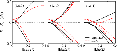
Figure 1: (Color online) Comparison of MBJLDA and LDA results for the $\Gamma_{8}$ band of YPtBi along high symmetry directions close to the $\Gamma$ point. The dotted line indicates the Fermi energy and $a$ is the lattice constant.

Generic ${\bf k}\cdot{\bf p}$ model for half-Heusler semimetals—Band structure calculations for YPtBi and LuPtBi indicate that the electronic states near the chemical potential arise from the $j=3/2$ $\Gamma_{8}$ representation, where the $j=3/2$ total angular momentum is due to the spin-orbit coupling of spin $s=1/2$ electrons in $l=1$ $p$-orbitals of Bi. In Fig. 5 we compare ab initio predictions for the $\Gamma_{8}$ band in YPtBi. We note that the band structure calculated using different exchange correlation potentials differ to some degree hhtop ; suppl . In particular, whereas the local-density approximation (LDA) predicts a compensated semimetal, the modified Becke and Johnson potential (MBJLDA) yields a zero band-gap semiconductor. The two schemes are in much better agreement for LuPtBi suppl . Further details of the ab initio calculations, including hybrid HSE06 functional results confirming the band inversion, are given in the supplemental material suppl . In either case it is possible to model the band structure near the $\Gamma$ point with a ${\bf k}\cdot{\bf p}$ theory. Such a theory was originally discussed by Dresselhaus dre55 ; up to quadratic order in $k$ the single-particle Hamiltonian is

$$H = \alpha k^{2}+\beta\sum_{i}k_{i}^{2}\check{J}_{i}^{2}{+\gamma\sum_{i\neq j}k_{i}k_{j}\check{J}_{i}\check{J}_{j}}$$ (1)

$$+\delta\sum_{i}k_{i}(\check{J}_{i+1}\check{J}_{i}\check{J}_{i+1}-\check{J}_{i+2}\check{J}_{i}\check{J}_{i+2})$$

where $i={x,y,z}$ and $i+1=y$ if $i=x$, etc., and $\check{J}_{i}$ are $4\times 4$ matrices corresponding to the angular momentum operators for $j=3/2$. The first line of Eq. (25) is the Luttinger-Kohn model, which is invariant under inversion and involves SSOC terms proportional to $\beta$ and $\gamma$. The second line is odd under inversion and generalizes the ASOC discussed in the context of $j=1/2$ noncentrosymmetric superconductors bau12 . Although this model qualitatively captures the predicted band structure, it is necessary to include higher-order terms in the ${\bf k}\cdot{\bf p}$ expansion to achieve quantitative agreement suppl . Since including these additional terms does not alter our conclusions about the superconductivity, but significantly complicates the analysis, we neglect them in the following.

Even with this simplification, it is not generally possible to analytically diagonalize the Hamiltonian (25). For our study of the superconductivity, however, we only require an effective low-energy model valid close to the Fermi surface. We obtain this by treating the ASOC as a perturbation of the Luttinger-Kohn bands, which is justified when the characteristic ASOC energy $\sim\delta k_{F}$ is small compared to the chemical potential measured from the four-fold degeneracy point. Experiments showing a low density of hole carriers but11 ; bay12 , and the predicted very weak ASOC splitting, are consistent with this condition.

The eigenstates of the Luttinger-Kohn model are doubly degenerate and can be labelled by pseudospin-$1/2$ indices. The dispersions are given by

$$\epsilon_{\bf k,\pm}=\left(\alpha+{\frac{5}{4}}\beta\right)|{\bf k}|^{2}\pm\beta\sqrt{\sum_{i}\left[k_{i}^{4}+\left(\tfrac{3\gamma^{2}}{\beta^{2}}-1\right)k_{i}^{2}k_{i+1}^{2}\right]}.$$ (2)

We now include the ASOC as a first-order perturbation by projecting the ASOC into the pseudospin basis for each band. We hence obtain two effective pseudospin-$1/2$ Hamiltonians

$$H_{\rm{eff},\pm}=\mathcal{P}_{\pm}\mathcal{U}^{\dagger}H\mathcal{U}\mathcal{P}_{\pm}=\epsilon_{\bf k,\pm}\hat{s}_{0}+{\bf g}_{{\bf k},\pm}\cdot\hat{\bf s}$$ (3)

where $\mathcal{P}_{\pm}$ projects into the pseudospin states of the $\epsilon_{{\bf k},\pm}$ bands (2), $\mathcal{U}$ is the unitary operator that diagonalizes $H$ with the ASOC set to zero, and $\hat{s}_{\mu}$ are the Pauli matrices for the pseudospin. The vector ${\bf g}_{{\bf k},\pm}=-{\bf g}_{-{\bf k},\pm}$ represents the effective ASOC in the pseudospin-$1/2$ basis of the band $\epsilon_{{\bf k},\pm}$. While the orientation of ${\bf g}_{{\bf k},\pm}$ depends on the arbitrary choice of pseudospin basis, the magnitude of ${\bf g}_{{\bf k},\pm}$ is independent of this choice and can be written

$$|{\bf g}_{\bf k,\pm}|^{2}=\frac{9\delta^{2}}{16}\left(\frac{\sum_{i}[(1+\frac{4\gamma^{2}}{\beta^{2}})k_{i}^{4}(k_{i+1}^{2}+k_{i+2}^{2})+(\frac{4\gamma^{2}}{\beta^{2}}-2)k_{i}^{2}k_{i+1}^{2}k_{i+2}^{2}]}{\sum_{i}\left[k_{i}^{4}+(\frac{3\gamma^{2}}{\beta^{2}}-1)k_{i}^{2}k_{i+1}^{2}\right]}\pm\frac{4\frac{\gamma}{\beta}\sum_{i}k_{i}^{2}k_{i+1}^{2}}{\sqrt{\sum_{i}\left[k_{i}^{4}+(\frac{3\gamma^{2}}{\beta^{2}}-1)k_{i}^{2}k_{i+1}^{2}\right]}}\right)$$ (4)

Note that along the $(1,1,1)$ direction this becomes $|{\bf g}_{{\bf k},\pm}|^{2}=\frac{3}{4}\delta^{2}k^{2}[1\pm\rm{sgn}(\gamma/\beta)]$, which is vanishing in one band but nonzero in the other. In the usual $j=1/2$ case, however, symmetry dictates that the ASOC must vanish along this direction bau12 ; the spin-orbit splitting of one of the bands therefore reflects the presence of $j=3/2$ physics even in our effective pseudospin-$1/2$ description. The effective Hamiltonians (3) can be readily diagonalized and yield the dispersions $E_{{\bf k},\eta=\pm,\nu=\pm}=\epsilon_{{\bf k},\eta}+\nu|{\bf g}_{{\bf k},\eta}|$, where the values of $\eta$ and $\nu$ are independent of one another. As shown in Fig. 2(a), this approximate dispersion is in excellent agreement with the full numerical solution of the ${\bf k}\cdot{\bf p}$ Hamiltonian, and yields typical spin-orbit split holelike Fermi surfaces plotted in Fig. 2(b).

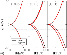
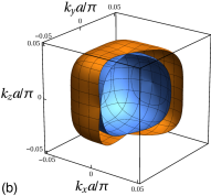
Figure 2: (Color online) (a) Comparison of exact and approximate small-ASOC dispersions along high symmetry directions. (b) Cut-away of spin-orbit-split holelike Fermi surfaces for $\mu=-20$meV. In all figures we take the parameters of the ${\bf k}\cdot{\bf p}$ Hamiltonian (25) to be $\alpha=20(a/\pi)^{2}$eV, $\beta=-15(a/\pi)^{2}$eV, $\gamma=-10(a/\pi)^{2}$eV, and $\delta=0.1(a/\pi)$eV.

Superconductivity—In the conventional theory of superconductivity, a Cooper pair constructed from two $j=1/2$ fermions has either total angular momentum $J=0$ (singlet) or $J=1$ (triplet), which by fermion antisymmetry correspond to even- and odd-parity orbital states, respectively. For the pairing of the $j=3/2$ states in the half-Heuslers, however, we must additionally allow for $J=2$ (quintet) and $J=3$ (septet) pairing, again corresponding to even- and odd-parity orbital wavefunctions. These extra pairing channels already manifest themselves in an expanded variety of on-site ($s$-wave) pairing: While there is a single $J=0$ state, there are five distinct types of on-site Cooper pair with $J=2$. The six local Cooper pair operators $b_{l,i}=\sum_{m,m^{\prime}}\Gamma^{l}_{m,m^{\prime}}c_{m,i}c_{m^{\prime},i}$ are defined and classified according to the tetrahedral point group symmetry in Table 1.

Representation	Cooper Pair	$J$
$A_{1}$	$c_{3/2}c_{-3/2}-c_{1/2}c_{-1/2}$	singlet
$E$	$c_{3/2}c_{-3/2}+c_{1/2}c_{-1/2}$	quintet
	$c_{3/2}c_{1/2}+c_{-1/2}c_{-3/2}$	quintet
$T_{2}$	$c_{3/2}c_{-1/2}+c_{1/2}c_{-3/2}$	quintet
	$-i\left(c_{3/2}c_{-1/2}-c_{1/2}c_{-3/2}\right)$	quintet
	$-i\left(c_{3/2}c_{1/2}-c_{-1/2}c_{-3/2}\right)$	quintet

Table 1: On-site Cooper pair operators for $j=3/2$ pairing. The first column gives the representation of $T_{d}$, the second shows the form of the local Cooper pair operator (with site index suppressed), and the last column gives the total angular momentum state.

In terms of these basis functions, the on-site pairing interaction will have the form $H_{\text{pair}}=\sum_{l}V_{l}b_{l,i}^{\dagger}b_{l,i}$ with one potential $V_{l}$ for each tetrahedral representation. Treating this within a usual mean-field theory yields a pairing term of the form

$$H_{\text{pair}}=\sum_{\bf k}\sum_{j,j^{\prime}=-3/2}^{3/2}\Big{\{}\Delta_{j,j^{\prime}}c^{\dagger}_{{\bf k},j}c^{\dagger}_{-{\bf k},j^{\prime}}+\text{H.c.}\Big{\}}.$$ (5)

It is instructive to project the $\Delta_{j,j^{\prime}}$ into the pseudospin basis of the $\epsilon_{{\bf k},\pm}$ bands, $\Delta_{\text{eff},\pm}({\bf k})=\mathcal{P}_{\pm}\mathcal{U}^{\dagger}\Delta\mathcal{U}^{*}\mathcal{P}_{\pm}$. In all cases the even parity of the pairing yields a pseudospin-singlet gap. Neglecting higher-order corrections, for on-site Cooper pairs in representation $A_{1}$, we find

$$\Delta^{A_{1}}_{\text{eff},\pm}=\Delta_{s}i\hat{s}_{y},$$ (6)

for on-site $E$ Cooper pairs we find

$$\Delta^{E}_{\text{eff},\pm}=\pm\frac{\beta}{4}\frac{\eta_{1}(2k_{z}^{2}-k_{x}^{2}-k_{y}^{2})+\eta_{2}\sqrt{3}(k_{x}^{2}-k_{y}^{2})}{\sqrt{\beta^{2}\sum_{i}k_{i}^{4}+(3\gamma^{2}-\beta^{2})\sum_{i}k_{i}^{2}k_{i+1}^{2}}}i\hat{s}_{y},$$ (7)

where ${\bm{\eta}}=(\eta_{1},\eta_{2})$ is a two-component order parameter, and for on-site $T_{2}$ Cooper pairs we find

$$\Delta^{T_{2}}_{\text{eff},\pm}=\pm\frac{\sqrt{3}\gamma}{2}\frac{l_{1}k_{y}k_{z}+l_{2}k_{x}k_{z}+l_{3}k_{x}k_{y}}{\sqrt{\beta^{2}\sum_{i}k_{i}^{4}+(3\gamma^{2}-\beta^{2})\sum_{i}k_{i}^{2}k_{i+1}^{2}}}i\hat{s}_{y},$$ (8)

which is characterized by the three-component order parameter $\bm{l}=(l_{1},l_{2},l_{3})$. The effective gaps of the quintet pairing states have $d$-wave form factors, which reflects the $J=2$ total angular momentum of the Cooper pairs. The $d$-wave symmetry is therefore a robust result, and does not depend on the specific parameters of our ${\bf k}\cdot{\bf p}$ Hamiltonian. Before discussing each of these cases in detail, we note an important property of the $E$ and $T_{2}$ states: The effective gaps, and therefore $T_{c}$, depend strongly on the SSOC terms in Eq. (25). Specifically, the effective gap for the $E$ states is vanishing unless $\beta\neq 0$, while the $T_{2}$ states only open a gap at the Fermi surface if $\gamma\neq 0$. Consequently, a spatial variation of the spin-orbit coupling (as might appear near surfaces or interfaces) can dramatically change $T_{c}$ for these solutions. We speculate that this may explain the enhanced $T_{c}$ observed at the surface of LuPtBi ak15 .

The $A_{1}$ pairing state—The on-site pairing in the $A_{1}$ channel corresponds to the conventional isotropic $s$-wave singlet state. It is therefore interesting to consider the effect of the broken inversion symmetry, which in $j=1/2$ noncentrosymmetric superconductors generates a mixed-parity state with both singlet and triplet pairing fri04 . For $T_{d}$ symmetry, the lowest orbital-angular-momentum $A_{1}$ triplet state is $f$-wave, which for small $k$ gives gap functions on the two spin-split $j=1/2$ Fermi surfaces $\Delta({\bf k})=\Delta_{s}\pm\Delta_{f}\sqrt{\sum_{i}k_{i}^{2}(k_{i+1}^{2}-k_{i+2}^{2})^{2}}$. This state exhibits line nodes if the $f$-wave triplet gap $\Delta_{f}$ is larger than the $s$-wave singlet gap $\Delta_{s}$. However, dominant $f$-wave symmetry of the Cooper pairs is highly unlikely if quasi-local interactions give rise to superconductivity kon89 ; such interactions would more plausibly give rise to a $p$-wave state. For the $j=3/2$ case considered here, however, a $p$-wave state with $A_{1}$ symmetry exists: In the basis $(c_{{\bf k},3/2},c_{{\bf k},1/2},c_{{\bf k},-1/2},c_{{\bf k},-3/2})$ it has gap function

$$\Delta({\bf k})=\Delta_{p}\left(\begin{array}[]{cccc}\frac{3}{4}k_{-}&\frac{\sqrt{3}}{2}k_{z}&\frac{\sqrt{3}}{4}k_{+}&0\\ \frac{\sqrt{3}}{2}k_{z}&\frac{3}{4}k_{+}&0&-\frac{\sqrt{3}}{4}k_{-}\\ \frac{\sqrt{3}}{4}k_{+}&0&-\frac{3}{4}k_{-}&\frac{\sqrt{3}}{2}k_{z}\\ 0&-\frac{\sqrt{3}}{4}k_{-}&\frac{\sqrt{3}}{2}k_{z}&-\frac{3}{4}k_{+}\\ \end{array}\right)$$ (9)

where $k_{\pm}=k_{x}\pm ik_{y}$. This constitutes a septet pairing state with total $J=3$. Projecting the gap into the effective pseudospin-$1/2$ bands, we find that $\Delta_{\text{eff},\pm}=({\bf d}_{{\bf k},\pm}\cdot\hat{\bf s})i\hat{s}_{y}=(\Delta_{p}/\delta)({\bf g}_{{\bf k},\pm}\cdot\hat{\bf s})i\hat{s}_{y}$, i.e. the ${\bf d}$-vector of the effective pseudospin-triplet state is parallel to the effective ASOC vector ${\bf g}_{{\bf k},\pm}$. As pointed out in LABEL:fri04, this alignment makes the gap $\Delta_{\text{eff},\pm}$ immune to the pair-breaking effect of the ASOC; for sufficiently large ASOC, it is the only stable odd-parity gap. Importantly, when mixed with a subdominant $s$-wave singlet state, the resulting gap displays line nodes on one of the spin-split Fermi surfaces, as shown in Fig. 3. These nodes are topologically protected and lead to zero-energy flat band surface states sch15 .

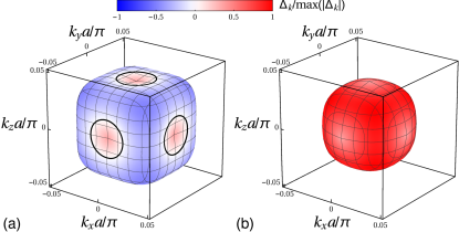
Figure 3: (Color online) Typical mixed singlet-septet $A_{1}$ pairing state with (a) a nodal gap on the larger Fermi surface and (b) a full gap on the smaller Fermi surface.

The $E$ pairing state—The properties of the $E$ superconducting state depends upon the two-dimensional order parameter ${\bm{\eta}}=(\eta_{1},\eta_{2})$. The free energy expansion for the $E$ pairing state in point group $T_{d}$ is the same as that for an $E_{g}$ state in point group $O_{h}$ sig91 , from which we deduce $f_{E}=\alpha{\bm{\eta}}\cdot{\bm{\eta}}^{*}+\beta_{1}({\bm{\eta}}\cdot{\bm{\eta}}^{*})^{2}+\beta_{2}(\eta_{1}\eta_{2}^{*}-\eta_{2}\eta_{1}^{*})^{2}$. In general there are three ground states: ${\bm{\eta}}=(1,0)$, $(0,1)$, and $(1,i)$. In the weak-coupling limit we find $\beta_{1}=3\beta_{2}>0$ independent of the particular form of the gap basis functions or the shape of the Fermi surface, ensuring that the TRSB state ${\bm{\eta}}=(1,i)$ is most stable. The effective gap, shown in Fig. 4(a), has topologically-protected Weyl point nodes that generate arc surface states sch15 . Although point nodes at first seem inconsistent with the observation of line nodes, it is possible that a point node state with impurities resembles a clean line node state nag15 ; hir88 , and hence it cannot be excluded as a possible pairing state in YPtBi.

The $T_{2}$ pairing state—The gap function for $T_{2}$ pairing is controlled by the three-dimensional order parameter $\bm{l}=(l_{1},l_{2},l_{3})$. Similar to the $E$ pairing state, the free energy expansion for the $T_{2}$ pairing in the $T_{d}$ point group is identical to that for $T_{2g}$ pairing in the point group $O_{h}$ sig91 , i.e. $f_{T_{2}}=\alpha\bm{l}\cdot\bm{l}^{*}+\beta_{1}(\bm{l}\cdot\bm{l}^{*})^{2}+\beta_{2}|\bm{l}\cdot\bm{l}|^{2}+\beta_{3}(|l_{1}|^{2}|l_{2}|^{2}+|l_{1}|^{2}|l_{3}|^{2}+|l_{3}|^{2}|l_{2}|^{2})$. This admits four distinct ground states: ${\bm{l}}=(1,0,0)$, $(1,1,1)$, $(1,e^{2\pi i/3},e^{4\pi i/3})$, or $(1,i,0)$. Again assuming weak coupling, the parameters in the free energy expansion satisfy $\beta_{1}>0$, $\beta_{2}>0$, and $\beta_{3}=2\beta_{2}-\beta_{1}$, which implies that one of the two TRSB states is realized. The particular state depends on the detailed form of the gap basis functions and the shape of the Fermi surface. We plot the corresponding effective gaps in Fig. 4(b) and (c). Both these gaps have interesting topological properties and surface states sch15 . Given that line nodes have been observed, the ${\bm{l}}=(1,i,0)$ solution is of particular interest.

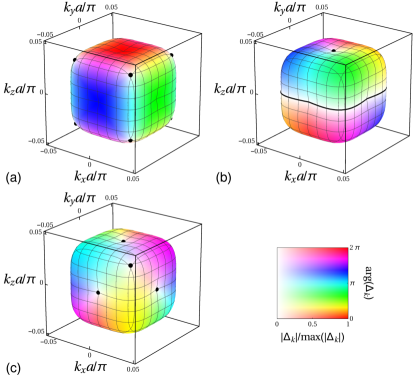
Figure 4: (Color online) Time-reversal symmetry-breaking quintet pairing states: (a) the $E$ pairing state; (b) the $T_{2}$ pairing state with ${\bf l}=(1,i,0)$; (c) the $T_{2}$ pairing state with ${\bf l}=(1,-e^{2\pi i/3},e^{4\pi i/3})$. The color indicates the phase while the saturation gives the gap magnitude. Black points or lines indicate nodes of the gap.

Conclusions—In this Letter we have investigated possible pairing states of the unconventional noncentrosymmetric superconductors YPtBi and LuPtBi. The inverted band structures of these topological semimetals implies pairing of $j=3/2$ fermions, permitting Cooper pairs in a quintet or septet total angular momentum state. On-site quintet pairing generically leads to nodal TRSB superconducting states, which could be detected by magneto-optical Kerr effect or $\mu$SR measurements. Alternatively, a nodal time-reversal symmetric gap can arise from the admixture of a $p$-wave septet state with an on-site singlet state. Spin-orbit coupling strongly influences the stability of these states. The similar electronic structure of the topological half-Heusler compounds makes our analysis relevant to the superconductivity of the entire materials class. Although we have not considered a pairing mechanism, the low carrier density makes a conventional Eliashberg theory unlikely mei15 . We note that pairing of $j=3/2$ fermions is not necessarily limited to the half-Heuslers: the four-fold degeneracy of the $\Gamma_{8}$ bands also occurs in materials with $O$, $T$, and $O_{h}$ point group symmetries, permitting the exotic superconducting states discussed here.

I Supplemental materials

II Derivation of the ${\bf k}\cdot{\bf p}$ Hamiltonian

The bands near the $\Gamma$ point are derived from the $\Gamma_{8}$ representation. A basis for this representation consists of the four the total angular momentum $j=3/2$ states $|3/2,m\rangle$ with $m=3/2,1/2,-1/2,-3/2$ book . To construct a $\bf{k}\cdot{\bf p}$ theory we need the sixteen operators that span the direct product space of $\Gamma_{8}\otimes\Gamma_{8}$. This can be conveniently done using powers of the $j=3/2$ operators $\check{J}_{i}$ which we list here in the $\{|3/2,3/2\rangle,|3/2,1/2\rangle,|3/2,-1/2\rangle,|3/2,-3/2\rangle\}$ basis ($\hbar=1$)

$$\check{J}_{x} = \frac{1}{2}\left(\begin{array}[]{cccc}0&\sqrt{3}&0&0\\ \sqrt{3}&0&2&0\\ 0&2&0&\sqrt{3}\\ 0&0&\sqrt{3}&0\\ \end{array}\right)$$ (14)

$$\check{J}_{y} = \frac{i}{2}\left(\begin{array}[]{cccc}0&-\sqrt{3}&0&0\\ \sqrt{3}&0&-2&0\\ 0&2&0&-\sqrt{3}\\ 0&0&\sqrt{3}&0\\ \end{array}\right)$$ (19)

$$\check{J}_{z} = \frac{1}{2}\left(\begin{array}[]{cccc}3&0&0&0\\ 0&1&0&0\\ 0&0&-1&0\\ 0&0&0&-3\\ \end{array}\right).$$ (24)

In particular, the relevant products can be constructed using the well known relationship for spherical symmetry $3/2\otimes 3/2=3\oplus 2\oplus 1\oplus 0$ and then decomposing the total $j$ states into tetrahedral representations. Using the character table for the tetrahedral group $T_{d}$ given in Table 2, we find: $j=0\rightarrow A_{1}$, $j=1\rightarrow T_{1}$, $j=2\rightarrow E\oplus T_{2}$, and $j=3\rightarrow A_{2}\oplus T_{1}\oplus T_{2}$. The corresponding operators are given in Table 3. In Table 3, we also give basis functions for the different tetrahedral representations for all power of $k_{i}$ up to the third power.

$REP$	$E$	$6C_{4}^{2}$	$8C_{3}$	$6S_{4}$	$6\sigma_{d}$
$A_{1}$	1	1	1	1	1
$A_{2}$	1	1	1	-1	-1
$E$	2	2	-1	0	0
$T_{1}$	3	-1	0	1	-1
$T_{2}$	3	-1	0	-1	1

Table 2: Character table for the Tetrahedral group $T_{d}$.

REP	$\check{J}_{i}$ basis functions	$k_{i}$ basis functions
$A_{1}$	$\check{J}_{x}^{2}+\check{J}_{y}^{2}+\check{J}_{z}^{2}=\frac{15}{4}\check{1}_{4}$	$k_{x}^{2}+k_{y}^{2}+k_{z}^{2}$, $k_{x}k_{y}k_{z}$
$A_{2}$	$\check{J}_{x}\check{J}_{y}\check{J}_{z}$ + symmetric permutations	-
$E$	$[(2\check{J}_{z}^{2}-\check{J}_{x}^{2}-\check{J}_{y}^{2})/\sqrt{3},\check{J}_{x}^{2}-\check{J}_{y}^{2}]$	$[(2k_{z}^{2}-k_{x}^{2}-k_{y}^{2})/\sqrt{3},k_{x}^{2}-k_{y}^{2}]$
$T_{1}$	$[\check{J}_{x},\check{J}_{y},\check{J}_{x}]$, $[\check{J}_{x}^{3},\check{J}_{y}^{3},\check{J}_{z}^{3}]$	$[k_{x}(k_{y}^{2}-k_{z}^{2}),k_{y}(k_{z}^{2}-k_{x}^{2}),k_{z}(k_{x}^{2}-k_{y}^{2})]$
$T_{2}$	$[\check{J}_{y}\check{J}_{x}\check{J}_{y}-\check{J}_{z}\check{J}_{x}\check{J}_{z},\check{J}_{z}\check{J}_{y}\check{J}_{z}-\check{J}_{x}\check{J}_{y}\check{J}_{x},\check{J}_{y}\check{J}_{z}\check{J}_{y}-\check{J}_{x}\check{J}_{z}\check{J}_{x}]$	$[k_{x},k_{y},k_{z}]$, $[k_{x}^{3},k_{y}^{3},k_{z}^{3}]$, $[k_{x}(k_{y}^{2}+k_{z}^{2}),k_{y}(k_{z}^{2}+k_{x}^{2}),k_{z}(k_{x}^{2}+k_{y}^{2})]$
	$[\check{J}_{y}\check{J}_{z}+\check{J}_{z}\check{J}_{y},\check{J}_{x}\check{J}_{z}+\check{J}_{z}\check{J}_{x},\check{J}_{x}\check{J}_{y}+\check{J}_{y}\check{J}_{x}]$	$[k_{y}k_{z},k_{x}k_{z},k_{x}k_{y}]$

Table 3: Tetrahedral basis functions for powers of $\check{J}_{i}$ and $k_{i}$

By forming all possible invariants from these powers of $k_{i}$ and the operators that span $\Gamma_{8}\otimes\Gamma_{8}$, we arrive at the ${\bf k}\cdot{\bf p}$ Hamiltonian

$$H = \alpha k^{2}+\beta\sum_{i}k_{i}^{2}\check{J}_{i}^{2}+\gamma\sum_{i\neq j}k_{i}k_{j}\check{J}_{i}\check{J}_{j}+\delta\sum_{i}k_{i}(\check{J}_{i+1}\check{J}_{i}\check{J}_{i+1}-\check{J}_{i+2}\check{J}_{i}\check{J}_{i+2})$$ (25)

$$+\epsilon_{1}\sum_{i}\check{J}_{i}k_{i}(k_{i+1}^{2}-k_{i+2}^{2})+\epsilon_{2}\sum_{i}\check{J}_{i}^{3}k_{i}(k_{i+1}^{2}-k_{i+2}^{2})+\epsilon_{3}\sum_{i}k_{i}^{3}(\check{J}_{i+1}\check{J}_{i}\check{J}_{i+1}-\check{J}_{i+2}\check{J}_{i}\check{J}_{i+2})$$

$$+\epsilon_{4}\sum_{i}k_{i}(k_{i+1}^{2}+k_{i+2}^{2})(\check{J}_{i+1}\check{J}_{i}\check{J}_{i+1}-\check{J}_{i+2}\check{J}_{i}\check{J}_{i+2})$$

where $i={x,y,z}$ and $i+1=y$ if $i=x$, etc. This Hamiltonian up to second order in the $k_{i}$ was initially discussed by Dresselhaus dre55 .

III Determination of the ${\bf k}\cdot{\bf p}$ Hamiltonian from band structures

The band structures of YPtBi and LuPtBi, including spin-orbit coupling, were calculated using several different approximations for exchange-correlation: (i) the standard PBE generalized gradient approximation parameterizationPBE (also referred to as “LDA”); (ii) the modified Becke-Johnson LDA MBJLDA potential that was developed to yield band gaps in better agreement with experiment for a wide class of materials; and the HSE06 hybrid functional HSE06 which includes a fraction (0.25) of exact exchange. For the MBJLDA, $\alpha$=0.012 and $\beta$=1.023 as given in Ref. MBJLDA were used.

In Fig. 5 we show the MBJLDA and LDA/GGA results for the $\Gamma_{8}$ bands of LuPtBi; the corresponding plot for YPtBi is shown in the main paper. Although there are differences in details that show up in the fitting parameters, the band topology is similar. Figure 6 compares the LDA/GGA bands to hybrid functional ones over a larger energy range, demonstrating that the band ordering is the same for all the different exchange-correlation choices with the $\Gamma_{8}$ states near the chemical potential. This result is not surprising since simple tight-binding arguments (without spin-orbit) predict that half-Heusler compounds with 18 valence electrons are (nearly zero-gap) semiconductors with the 6-fold $\Gamma_{15}$ (3-dimensional representation $\times$ 2 for spin) state at/near $E_{F}$. Inclusion of spin-orbit does not alter this picture: Spin-orbit pushes the 2-fold $\Gamma_{7}$ state (with its downward dispersing bands) to lower energy, while the 4-fold $\Gamma_{8}$ states remain near $E_{F}$. Thus, although there are differences in the band dispersions, the overall band topologies are the same. In particular, any reasonable calculation of these half-Heusler materials will lead to the $j=3/2$ $\Gamma_{8}$ states near the chemical potential, which is the essential aspect needed for the superconductivity discussed here.

In the following we carry out detailed fits to only the MBJLDA and LDA results. The two schemes are in much better agreement for LuPtBi than for YPtBi (shown in the main paper). From fitting the band structures near the $\Gamma$ point we can extract the parameters in the ${\bf k}\cdot{\bf p}$ Hamiltonian. To carry out these fits, we first extracted the parameters $\alpha$, $\beta$, $\gamma$, and $\delta$. We found that we needed to also include the cubic term $\epsilon_{1}$ to correctly model the bands in the $(1,1,0)$ direction. The other cubic parameters we set to zero. The resultant parameters are given in Table 4. In addition, we note that the inclusion of quartic terms is required to capture an additional electron pocket that appears near the calculated Fermi energy for some of the density functional calculations. Early experimental results suggest that these materials are hole doped but11 ; bay12 , so it is likely that this electron Fermi surface does not appear in the superconducting materials. However, we note that our main results: the appearance of nodal broken time-reversal $d$-wave quintet pairing states and the existence of a mixed $s$-wave singlet and $p$-wave septet state with topologically protected line nodes are not affected by this additional electron pocket.

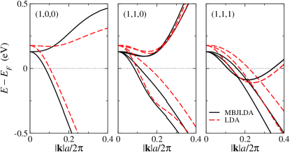
Figure 5: (Color online) Comparison of MBJLDA and LDA (PBE GGA) results for the $\Gamma_{8}$ band of LuPtBi along high symmetry directions close to the $\Gamma$ point. The dotted line indicates the Fermi energy and $a$ is the lattice constant. A similar plot for YPtBi is given in the main paper.

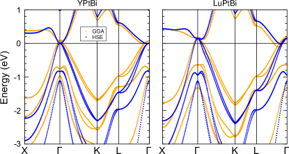
Figure 6: (Color online) Comparison of the calculated YPtBi and LuPtBi relativistic band structures around the Fermi level using the PBE GGA (orange) and the HSE06 hybrid (blue) functionals. Although the hybrid functional tends to push the valence states at the zone boundary deeper, the ordering of the states remains the same.

Material	Potential	$\alpha$	$\beta$	$\gamma$	$\delta$	$\epsilon_{1}$
		($eVa^{2}/\pi^{2}$)	($eVa^{2}/\pi^{2}$)	($eVa^{2}/\pi^{2}$))	($eVa/\pi$)	($eVa^{3}/\pi^{3}$)
YPtBi	LDA	8.2	-11.6	1.7	0.01	73
YPtBi	MBJLDA	20.5	-18.5	-1.27	0.025	45
LuPtBi	LDA	0.48	-8.7	5.3	0.11	70
LuPtBi	MBJLDA	5.32	-13.9	4.2	0.12	80

Table 4: ${\bf k}\cdot{\bf p}$ fitting parameters for different band structures for YPtBi and LuPtBi.

References

- (1) G.F. Koster, J.O. Dimmock, R.G. Wheeler, and H. Statz, Properties of the thirty-two point groups, MIT Press, Cambridge, Mass. (1963).
- (2) G. Dresselhaus, Phys. Rev. 100, 580 (1955).
- (3) J. P. Perdew, K. Burke, and M. Ernzerhof, Phys. Rev. Lett. 77, 3865 (1996); 78, 1396 (1997).
- (4) F. Tran and P. Blaha, Phys. Rev. Lett. 102, 226401 (2009).
- (5) J. Heyd, J. E. Peralta, G. E. Scuseria, and R. L. Martin, J. Chem. Phys. 123, 174101 (2005).
- (6) N. P. Butch, P. Syers, K. Kirshenbaum, A. P. Hope, and J. Paglione, Phys. Rev. B 84, 220504(R) (2011).
- (7) T. V. Bay, T. Naka, Y. K. Huang, and A. de Visser, Phys. Rev. B 86, 064515 (2012).