Interrupted orbital motion in density-wave systems

Abstract

In conventional metals, electronic transport in a magnetic field is characterized by the motion of electrons along orbits on the Fermi surface, which usually causes an increase in the resistivity through averaging over velocities. Here we show that large deviations from this behavior can arise in density-wave systems close to their ordering temperature. Specifically, enhanced scattering off collective fluctuations can lead to a change of direction of the orbital motion on reconstructed pockets. In weak magnetic fields, this leads to linear magnetoconductivity, the sign of which depends on the electric-field direction. At a critical magnetic field, the conductivity crosses zero for certain directions, signifying a thermodynamic instability of the density-wave state.

I Introduction

The central concept in the theory of magnetotransport in metals is the motion of electrons along the Fermi surface, driven by the Lorentz force. This is described by the semiclassical equation of motion

$$\frac{d}{dt}\,\hbar\mathbf{k}=-e\,\mathbf{v}_{\mathbf{k}}\times\mathbf{B},$$ (1)

where $\hbar\mathbf{k}$ is the momentum at the Fermi surface, $-e$ is the electron charge, and $\mathbf{v}_{\mathbf{k}}=\nabla_{\mathbf{k}}\varepsilon_{\mathbf{k}}/\hbar$ is the velocity for the dispersion $\varepsilon_{\mathbf{k}}$. The direction of the Lorentz force is opposite for electron-like and hole-like Fermi pockets since $\mathbf{v}_{\mathbf{k}}$ is opposite.

The driving by the Lorentz force is balanced by various scattering mechanisms, which also have a profound effect on the motion of the electrons in momentum space. Most theoretical investigations consider the case that the scattering is approximately isotropic so that one can identify the electronic lifetime with the transport relaxation time, i.e., the time needed to randomize the velocity of the electron. In this case, the shift of the electron is obtained by integrating Eq. (1) over the lifetime, hence its direction is obviously set by the Lorentz force.

The presence of anisotropic scattering significantly complicates this picture, as we can no longer simply integrate Eq. (1). This is an important problem, as strong anisotropic scattering is expected in a number of materials of current interest, in particular in excitonic systems such as transition-metal dichalcogenidesRossnagel (2011); Ganesh et al. (2014); Kim et al. (2015); Eom et al. (2014) and iron pnictides.Johnston (2010); Chubukov (2012); Stewart (2011); Fernandes et al. (2014); Yin et al. (2014) Here, nesting of electron-like and hole-like Fermi pockets in the disordered stateInosov et al. (2008); Rossnagel (2011); Mazin and Schmalian (2009) favors the condensation of electron-hole pairs (interband excitons) due to repulsive electronic interactions, which can drive the system into a density-wave state with ordering vector equal to the nesting vector.Han et al. (2008); Chubukov et al. (2008); Vorontsov et al. (2009); Brydon and Timm (2009); Eremin and Chubukov (2010); Brydon et al. (2011)

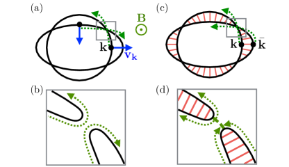
Figure 1: (Color online) (a) Nearly nested electron-like and hole-like pockets (solid black lines) of an excitonic system in a backfolded Brillouin zone. Dotted arrows denote the directions of orbital motion in the absence of anisotropic scattering. (b) Close-up of the intersection, where the reconstruction below the transition sets in. (c), (d) Same as (a), (b), respectively, but in the presence of anisotropic scattering between the states $|\mathbf{k}\rangle$ and $|{\bar{\mathbf{k}}}\rangle$, indicated by the red (gray) bars. The orbital motion on one of the pockets is reversed. In (d), the emergence of points at which the effective orbital motion changes direction leads to singularities.

The Fermi pockets of a minimal model in the disordered state are sketched in Fig. 1(a), where the Brillouin zone has been backfolded according to the nesting vector. The density-wave order leads to a reconstruction of the Fermi pockets which sets in at their intersections, as sketched in Fig. 1(b). This results in two electron-like and two hole-like banana-shaped pockets, which have large portions that are dominated by the states of the original electron-like or hole-like Fermi surfaces, and small turning regions with mixed character near the gapped-out intersections. Anisotropic scattering between the approximately nested parts of the Fermi pockets is mediated by enhanced collective fluctuations, which are particularly strong close to the transition. Scattering due to these fluctuations is thought to be responsible for unconventional Cooper pairingMazin and Schmalian (2009); Chubukov (2012); Graser et al. (2009); *Graser2010; Kuroki et al. (2009); Ikeda et al. (2010); Schmiedt et al. (2014) and transport anomalies in the normal state.Rullier-Albenque et al. (2012); Ohgushi and Kiuchi (2012); Fernandes et al. (2011); Fanfarillo et al. (2012); Breitkreiz et al. (2013, 2014a, 2014b)

In this work, we focus on the impact of anisotropic scattering on the orbital motion beyond the lifetime approximation. Due to the quasi-two-dimensional nature of many density-wave materials, we develop our theory for a two-dimensional model with out-of-plane magnetic field $\mathbf{B}$. Before giving an in-depth discussion, we first explain the results in qualitative terms. The strong collective fluctuations near the density-wave transition mediate strong scattering between states with momentum transfer close to the nesting vector. These pairs of states, denoted by $|\mathbf{k}\rangle$ and $|{\bar{\mathbf{k}}}\rangle$, are connected by the red (gray) bars in Figs. 1(c) and 1(d). The relevant timescale for the orbital motion is set by the transport relaxation time, which for strongly anisotropic scattering is much longer than the timescale of the scattering between $|\mathbf{k}\rangle$ and $|{\bar{\mathbf{k}}}\rangle$.Breitkreiz et al. (2013, 2014a) Thus, before integrating the equation of motion (1) over the relaxation time, the Lorentz force should first be averaged over these two states. While the bare Lorentz force is nearly antiparallel for $|\mathbf{k}\rangle$ and $|{\bar{\mathbf{k}}}\rangle$, the averaged Lorentz force is the same for both. Consequently, the direction of the orbital motion must be reversed for one of the two states.

Specifically in the density-wave state, there is strong scattering between states on opposite sides of the same reconstructed pocket. Consequently, a reversal of the effective orbital motion of electrons starting on one of the sides can occur. This implies that the effective orbital motion changes its direction in the turning region and so there has to exist a point where it vanishes. This interrupted orbital motion is our central result, which leaves unambiguous signatures in the magnetoconductivity. Note that at the points of interruption, the electronic lifetimes are generically not suppressed, which is a crucial difference to the previously proposed possible interruption in systems with hot spots on the Fermi surface.Koshelev (2013)

In the next section we present a detailed description of the mechanism leading to the interrupted orbital motion. In Sec. III we then discuss the most dramatic consequence of the interruption—negative longitudinal conductivity and the associated instability of the density-wave state. In Secs. IV and V we explicitly calculate the magnetoresistance for a two-pocket and a four-pocket model, respectively. We summarize our work and draw conclusions in Sec. VI.

 

II Interrupted orbital motion

We now describe the interrupted orbital motion in more detail, using the semiclassical transport formalism.Taylor (1963) Standard approximation schemes, such as the relaxation-time approximation, are ill suited for the analysis of strongly anisotropic scattering.Pikulin et al. (2011) In this work, we instead utilize an approximation that becomes exact in the limit of strong anisotropy.Breitkreiz et al. (2013, 2014a)

Our starting point is the Boltzmann equation for the stationary non-equilibrium distribution function $f_{\mathbf{k}}$,

$$(-e\mathbf{E}-e\mathbf{v}_{\mathbf{k}}\times\mathbf{B})\cdot\frac{1}{\hbar}\nabla_{\mathbf{k}}f_{\mathbf{k}}=\sum_{\mathbf{k}^{\prime}}W_{\mathbf{k}}^{\mathbf{k}^{\prime}}\,(f_{\mathbf{k}^{\prime}}-f_{\mathbf{k}}),$$ (2)

where detailed balance requires the scattering rates $W_{\mathbf{k}}^{\mathbf{k}^{\prime}}$ to be symmetric in $\mathbf{k}$ and $\mathbf{k}^{\prime}$. The distribution function can be written as $f_{\mathbf{k}}=n_{F}(\varepsilon_{\mathbf{k}})-n^{\prime}_{F}(\varepsilon_{\mathbf{k}})\,(-e)\,\mathbf{E}\cdot\mathbf{\Lambda}_{\mathbf{k}}$ up to linear order in the electric field $\mathbf{E}$.Price (1957); *Price1958; Taylor (1963) Here, $n_{F}(\varepsilon_{\mathbf{k}})$ is the Fermi function and $\mathbf{\Lambda}_{\mathbf{k}}$ is the vector mean free path (MFP). A standard derivation then givesTaylor (1963)

$$\mathbf{\Lambda}_{\mathbf{k}}=\tau_{0,\mathbf{k}}\mathbf{v}_{\mathbf{k}}+\tau_{0,\mathbf{k}}\,\frac{e}{\hbar}[(\mathbf{v}_{\mathbf{k}}\times\mathbf{B})\cdot\nabla_{\mathbf{k}}]\,\mathbf{\Lambda}_{\mathbf{k}}+\tau_{0,\mathbf{k}}\sum_{\mathbf{k}^{\prime}}W_{\mathbf{k}}^{\mathbf{k}^{\prime}}\mathbf{\Lambda}_{\mathbf{k}^{\prime}},$$ (3)

with the lifetime $\tau_{0,\mathbf{k}}\equiv(\sum_{\mathbf{k}^{\prime}}W_{\mathbf{k}}^{\mathbf{k}^{\prime}})^{-1}$. We parametrize the momenta along a Fermi pocket by $\mathbf{k}=\mathbf{k}(\alpha)$ and choose $\alpha$ to increase in the direction opposite to the direction of orbital motion, which is given by $-e\,\mathbf{v}_{\mathbf{k}}\times\mathbf{B}$. Then Eq. (3) becomes

$$\mathbf{\Lambda}_{\mathbf{k}}=\tau_{0,\mathbf{k}}\mathbf{v}_{\mathbf{k}}+\tau_{0,\mathbf{k}}\,\omega_{0,\mathbf{k}}\,\partial_{\alpha}\mathbf{\Lambda}_{\mathbf{k}}+\tau_{0,\mathbf{k}}\sum_{\mathbf{k}^{\prime}}W_{\mathbf{k}}^{\mathbf{k}^{\prime}}\mathbf{\Lambda}_{\mathbf{k}^{\prime}},$$ (4)

where $\omega_{0,\mathbf{k}}\equiv(e/\hbar)\,(\mathbf{v}_{\mathbf{k}}\times\mathbf{B})\cdot\nabla_{\mathbf{k}}\alpha>0$ is the cyclotron frequency.

For later comparison, we first consider the case of isotropic scattering. If $W_{\mathbf{k}}^{\mathbf{k}^{\prime}}$ is independent of $\mathbf{k}^{\prime}$ and the system satisfies inversion symmetry, the sum in Eq. (4) vanishes, and one obtains

$$\mathbf{\Lambda}_{\mathbf{k}}=\tau_{0,\mathbf{k}}\,\big{(}\mathbf{v}_{\mathbf{k}}+\omega_{0,\mathbf{k}}\,\partial_{\alpha}\mathbf{\Lambda}_{\mathbf{k}}\big{)}.$$ (5)

The derivative term accounts for the deviation of the MFP from its zero-field value $\mathbf{\Lambda}^{(0)}_{\mathbf{k}}=\tau_{0,\mathbf{k}}\mathbf{v}_{\mathbf{k}}$ due to the orbital motion. This motion is characterized by the cyclotron frequency $\omega_{0,\mathbf{k}}$, which only depends on the band parameters at $\mathbf{k}$. Equation (5) is solved by the “Shockley tube integral”Shockley (1950); Koshelev (2013)

$$\mathbf{\Lambda}_{\mathbf{k}} = \int_{\alpha}^{\infty}\!\!d\alpha^{\prime}\,\mathbf{\Lambda}_{\mathbf{k}^{\prime}}^{(0)}$$ (6)

$${}\times\underbrace{\frac{1}{\tau_{0,\mathbf{k}^{\prime}}\,\omega_{0,\mathbf{k}^{\prime}}}\,\exp\bigg{(}-\int_{\alpha}^{\alpha^{\prime}}\!\!d\alpha^{\prime\prime}\frac{1}{\tau_{0,\mathbf{k}^{\prime\prime}}\,\omega_{0,\mathbf{k}^{\prime\prime}}}\bigg{)}}_{\equiv\,D_{0,\alpha}(\alpha^{\prime})}.\leavevmode\nobreak\$$

The integration over $\alpha^{\prime}$ starts from the state $|\mathbf{k}\rangle$ and wraps around the pocket infinitely many times. The expression $D_{0,\alpha}(\alpha^{\prime})$ is a distribution function over the integration range $[\alpha,\infty)$, which corresponds to all previous states of the orbital motion ending up at $\mathbf{k}(\alpha)$. For vanishing field (i.e., $\omega_{0,\mathbf{k}}\to 0$) the weight is concentrated at $|\mathbf{k}\rangle$, while for increasing field the weight becomes more and more evenly distributed over the pocket.

For general scattering rates, a closed-form solution of Eq. (4) does not exist. However, it is possible to find an approximate solution that becomes exact in the limit of strongly anisotropic scattering. As the first step, we iterate Eq. (4), which yields

$$\mathbf{\Lambda}_{\mathbf{k}}=\tau_{0,\mathbf{k}}\sum_{\mathbf{k}^{\prime}}\pi_{\mathbf{k}}(\mathbf{k}^{\prime})\left(\mathbf{v}_{\mathbf{k}^{\prime}}+\omega_{0,\mathbf{k}^{\prime}}\,\partial_{\alpha^{\prime}}\mathbf{\Lambda}_{\mathbf{k}^{\prime}}\right),$$ (7)

with

$$\pi_{\mathbf{k}}(\mathbf{k}^{\prime})\equiv\delta_{\mathbf{k},\mathbf{k}^{\prime}}+W_{\mathbf{k}}^{\mathbf{k}^{\prime}}\tau_{0,\mathbf{k}^{\prime}}+\sum_{\mathbf{k}_{1}}W_{\mathbf{k}}^{\mathbf{k}_{1}}\tau_{0,\mathbf{k}_{1}}W_{\mathbf{k}_{1}}^{\mathbf{k}^{\prime}}\tau_{0,\mathbf{k}^{\prime}}+\ldots$$ (8)

This is a geometric series of the matrix with entries $W_{\mathbf{k}}^{\mathbf{k}^{\prime}}\tau_{0,\mathbf{k}^{\prime}}$. However, since this matrix has an eigenvalue of unity, with left eigenvector $(1,1,\ldots)$, the series does not converge. To solve this problem, we assume inversion symmetry and redefine $\pi_{\mathbf{k}}(\mathbf{k}^{\prime})$ by subtracting the isotropic contribution to the scattering,

$$\pi_{\mathbf{k}}(\mathbf{k}^{\prime})\equiv\delta_{\mathbf{k},\mathbf{k}^{\prime}}+W_{\mathbf{k}}^{\mathbf{k}^{\prime}}\tau_{0,\mathbf{k}^{\prime}}-c_{\mathbf{k}}$$ (9)

$$\quad{}+\sum_{\mathbf{k}_{1}}\left(W_{\mathbf{k}}^{\mathbf{k}_{1}}\tau_{0,\mathbf{k}_{1}}-c_{\mathbf{k}}\right)\left(W_{\mathbf{k}_{1}}^{\mathbf{k}^{\prime}}\tau_{0,\mathbf{k}^{\prime}}-c_{\mathbf{k}_{1}}\right)+\ldots,\qquad$$

where $c_{\mathbf{k}}\equiv\min_{\mathbf{k}^{\prime}}W_{\mathbf{k}}^{\mathbf{k}^{\prime}}\tau_{0,\mathbf{k}^{\prime}}$, which ensures that $\pi_{\mathbf{k}}(\mathbf{k}^{\prime})\geq 0$. Since $\mathbf{v}_{\mathbf{k}}$ and $\omega_{0,\mathbf{k}}\partial_{\alpha}\mathbf{\Lambda}_{\mathbf{k}}$ are odd under inversion, $c_{\mathbf{k}}$ drops out of Eq. (7). Equation (9) is again a geometric series of matrices. Their components are non-negative and the row sums are $\sum_{\mathbf{k}}(W_{\mathbf{k}}^{\mathbf{k}^{\prime}}\tau_{0,\mathbf{k}^{\prime}}-c_{\mathbf{k}})=1-\sum_{\mathbf{k}}c_{\mathbf{k}}$, which is smaller than unity if there exists a $c_{\mathbf{k}}>0$. The spectral radius of the matrix is then smaller than unity and the series converges. With the help of the normalization factor $N_{\mathbf{k}}\equiv\sum_{\mathbf{k}^{\prime}}\pi_{\mathbf{k}}(\mathbf{k}^{\prime})$, we then define the distribution function $P_{\mathbf{k}}(\mathbf{k}^{\prime})\equiv\pi_{\mathbf{k}}(\mathbf{k}^{\prime})/N_{\mathbf{k}}$ and the relaxation time $\tau_{\mathbf{k}}\equiv N_{\mathbf{k}}\,\tau_{0,\mathbf{k}}$. With this, Eq. (7) becomes

$$\mathbf{\Lambda}_{\mathbf{k}}=\tau_{\mathbf{k}}\sum_{\mathbf{k}^{\prime}}P_{\mathbf{k}}(\mathbf{k}^{\prime})\left(\mathbf{v}_{\mathbf{k}^{\prime}}+\omega_{0,\mathbf{k}^{\prime}}\,\partial_{\alpha^{\prime}}\mathbf{\Lambda}_{\mathbf{k}^{\prime}}\right),$$ (10)

which is a plausible generalization of Eq. (5)—the lifetime is replaced by the relaxation time and the term in parentheses is averaged over final states.

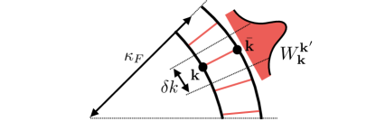
Figure 2: (Color online) Sketch of a segment of a reconstructed pocket. The scattering rate $W_{\mathbf{k}}^{\mathbf{k}^{\prime}}$ is peaked at $\mathbf{k}^{\prime}={\bar{\mathbf{k}}}$ with peak width $\delta k$, which is much smaller than the radius of curvature of the pocket, $\kappa_{F}$.

We now apply the general expression (10) to the specific situation in excitonic systems close to their density-wave instability. Here, the approximate nesting of electron and hole pockets enhances collective fluctuations, which mediate single-particle scattering between the pockets.Fernandes et al. (2011); Fanfarillo et al. (2012); Breitkreiz et al. (2014a) Qualitatively, this results in a scattering rate $W_{\mathbf{k}}^{\mathbf{k}^{\prime}}$ with a narrow peak at $\mathbf{k}^{\prime}={\bar{\mathbf{k}}}$, as sketched in Fig. 2.

Here, we consider the strongly anisotropic limit of this situation, i.e., we assume that the peak width $\delta k$ is much smaller than the radius of curvature of the pocket, $\kappa_{F}$. We further assume that an electron repeatedly hopping between the states given by the maximum of $W_{\mathbf{k}}^{\mathbf{k}^{\prime}}$ is always found in one of the two states $|\mathbf{k}\rangle$ or $|{\bar{\mathbf{k}}}\rangle$, i.e., $\bar{{\bar{\mathbf{k}}}}=\mathbf{k}$. This is true for perfectly nested pockets, whereas imperfect nesting can induce an additional shift along the pocket.Breitkreiz et al. (2014a); Varma and Abrahams (2001) However, for nearly nested pockets this shift is smallBreitkreiz et al. (2014a) and we therefore neglect it in the following.

For this specific form of $W_{\mathbf{k}}^{\mathbf{k}^{\prime}}$, the distribution $P_{\mathbf{k}}(\mathbf{k}^{\prime})$ has narrow peaks at $\mathbf{k}^{\prime}=\mathbf{k}$ and $\mathbf{k}^{\prime}={\bar{\mathbf{k}}}$. The leading-order term in $\delta k/\kappa_{F}$ is obtained by considering $W_{\mathbf{k}}^{\mathbf{k}^{\prime}}$ to be a $\delta$-function. Including also an isotropic contribution, we write $W_{\mathbf{k}}^{\mathbf{k}^{\prime}}=w_{a,\mathbf{k}}\delta_{\mathbf{k}^{\prime},{\bar{\mathbf{k}}}}+w_{i}/N$. Here, $N$ is the number of $\mathbf{k}$ points and is included to regularize the momentum sum in the lifetime $\tau_{0,\mathbf{k}}=1/\sum_{\mathbf{k}^{\prime}}W_{\mathbf{k}}^{\mathbf{k}^{\prime}}=1/(w_{a,\mathbf{k}}+w_{i})$. Detailed balance requires $w_{a,\mathbf{k}}=w_{a,{\bar{\mathbf{k}}}}$. For simplicity, we assume the strength of anisotropic scattering to be momentum independent, $w_{a,\mathbf{k}}=w_{a}$. We then find

$$P_{\mathbf{k}}(\mathbf{k}^{\prime})=\frac{w_{a}+w_{i}}{2w_{a}+w_{i}}\,\delta_{\mathbf{k}^{\prime},\mathbf{k}}+\frac{w_{a}}{2w_{a}+w_{i}}\,\delta_{\mathbf{k}^{\prime},{\bar{\mathbf{k}}}}$$ (11)

and $\tau_{\mathbf{k}}=1/w_{i}$. As expected, the distribution function has two peaks. On the other hand, the relaxation time is determined by the isotropic part of the scattering, which alone ensures a randomization of the velocity. Equation (10) shows that in the highly anisotropic limit, $w_{i}\ll w_{a}$, the MFPs $\mathbf{\Lambda}_{\mathbf{k}}$ and $\mathbf{\Lambda}_{{\bar{\mathbf{k}}}}$ become equal and we obtain

$$\mathbf{\Lambda}_{\mathbf{k}}=\mathbf{\Lambda}^{(0)}_{\mathbf{k}}+\tau_{\mathbf{k}}\,\omega_{\mathbf{k}}\,\partial_{\alpha}\mathbf{\Lambda}_{\mathbf{k}},$$ (12)

where the zero-field MFP reads $\mathbf{\Lambda}^{(0)}_{\mathbf{k}}=\tau_{\mathbf{k}}\,(\mathbf{v}_{\mathbf{k}}+\mathbf{v}_{{\bar{\mathbf{k}}}})/2$. The effect of the magnetic field is governed by the effective cyclotron frequency $\omega_{\mathbf{k}}\equiv(\omega_{0,\mathbf{k}}-\omega_{0,{\bar{\mathbf{k}}}})/2$, where we employ a parametrization such that $\partial_{\alpha}\bar{\alpha}=-1$ for convenience. Note that since the parameter $\alpha$ changes monotonically around the Fermi pocket, the parameter $\bar{\alpha}$ belonging to ${\bar{\mathbf{k}}}$ decreases if $\alpha$ increases. The strong scattering between $|\mathbf{k}\rangle$ and $|{\bar{\mathbf{k}}}\rangle$ is reflected by the mixing of the bare cyclotron frequencies $\omega_{0,\mathbf{k}}$ and $\omega_{0,{\bar{\mathbf{k}}}}$. The effective frequency $\omega_{\mathbf{k}}$ clearly has opposite signs for the states $|\mathbf{k}\rangle$ and $|{\bar{\mathbf{k}}}\rangle$, in contrast to the positive bare frequencies.

Above the transition, the states $|\mathbf{k}\rangle$ and $|{\bar{\mathbf{k}}}\rangle$ lie on two separate pockets of different (electron or hole) type, which implies opposite signs of $\omega_{\mathbf{k}}$ for these pockets. Assuming that there are no sign changes in $\omega_{\mathbf{k}}$ within a single pocket, the solution for the MFP has the usual form of the Shockley tube integral, Eq. (6), but with $\tau_{0,\mathbf{k}}\,\omega_{0,\mathbf{k}}$ replaced by $\tau_{\mathbf{k}}\,\omega_{\mathbf{k}}$ and the upper limit of the integral, $\infty$, replaced by $\infty\,\mathrm{sgn}\,\omega_{\mathbf{k}}$. For $\omega_{\mathbf{k}}<0$, the direction of the integration path is thus reversed, indicating reversed orbital motion for electrons originating on the corresponding pocket.Breitkreiz et al. (2014a)

The situation becomes even more interesting if there are sign changes in $\omega_{\mathbf{k}}$ within a single pocket. This generically happens below the transition, as the states $|\mathbf{k}\rangle$ and $|{\bar{\mathbf{k}}}\rangle$ now lie on the same reconstructed pocket. At a turning point, denoted by $\mathbf{k}_{t}$, the two peaks in $P_{\mathbf{k}}(\mathbf{k}^{\prime})$ merge so that $\mathbf{k}_{t}={\bar{\mathbf{k}}}_{t}$ and consequently $\omega_{\mathbf{k}_{t}}=0$. The solution of Eq. (12) is then

$$\mathbf{\Lambda}_{\mathbf{k}}=\int_{\alpha}^{\alpha_{t}}\!\!d\alpha^{\prime}\,\mathbf{\Lambda}_{\mathbf{k}^{\prime}}^{(0)}\underbrace{\frac{1}{\tau_{\mathbf{k}^{\prime}}\,\omega_{\mathbf{k}^{\prime}}}\,\exp\bigg{(}-\int_{\alpha}^{\alpha^{\prime}}\!\!d\alpha^{\prime\prime}\frac{1}{\tau_{\mathbf{k}^{\prime\prime}}\,\omega_{\mathbf{k}^{\prime\prime}}}\bigg{)}}_{\equiv\,D_{\alpha}(\alpha^{\prime})},$$ (13)

where the upper limit $\alpha_{t}$ corresponds to the first turning point reached from the starting point $\alpha$ backward in time (since the integral is over previous states of an electron). The direction of integration is set by the sign of the effective cyclotron frequency: $\mathrm{sgn}\,(\alpha_{t}-\alpha)=\mathrm{sgn}\,\omega_{\mathbf{k}}$. The cutoff $\alpha_{t}$ is the crucial difference to the usual tube integral, Eq. (6), and signals the interrupted orbital motion. The weight of the distribution function $D_{\alpha}(\alpha^{\prime})$ is now restricted to the range $[\alpha,\alpha_{t})$, as sketched in Fig. 3. For strong magnetic fields, i.e., $\tau_{\mathbf{k}}\,\omega_{\mathbf{k}}\gg 1$, the weight completely shifts towards the repulsive turning point, i.e., the one the electrons move away from, and we thus find $\mathbf{\Lambda}_{\mathbf{k}}\approx\mathbf{\Lambda}^{(0)}_{\mathbf{k}_{t}}$, implying that the MFPs of all states on a single pocket approach the MFP at the turning point. This is the turning point the electrons move away from.

The points of interruption are those points on the Fermi surface where the factor $\tau_{\mathbf{k}}\,\omega_{\mathbf{k}}$ is zero, associated with a sign change of $\tau_{\mathbf{k}}\,\omega_{\mathbf{k}}$. The crucial ingredient for these zeros is the strongly anisotropic scattering between quasi-nested Fermi surfaces. A different and, so to speak, weaker interruption of orbital motion can occur in systems with hot spots on the Fermi surface.Koshelev (2013) Here, the factor $\tau_{\mathbf{k}}\,\omega_{\mathbf{k}}$ can be strongly suppressed by the very short relaxation time at hot spots, which however remains nonzero. Since in this case $\tau_{\mathbf{k}}\,\omega_{\mathbf{k}}$ has no sign changes, the tube integral has the conventional form, Eq. (6), without a cutoff.

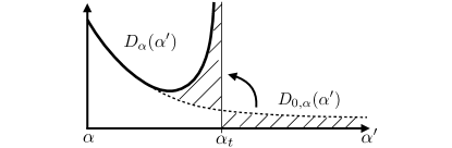
Figure 3: Sketch of the distribution function $D_{\alpha}(\alpha^{\prime})$ for the case of orbital motion interrupted at $\alpha_{t}$. The weight, which in the absence of interruption was spread over $[\alpha,\infty)$ ($D_{0,\alpha}(\alpha^{\prime})$, dashed line), is now restricted to the range $[\alpha,\alpha_{t})$.

 

III Negative longitudinal conductivity

One of the most dramatic consequences of the interrupted orbital motion is the possibility of negative longitudinal conductivity. In the following, we discuss the general ideas before turning to the conductivity for specific models.

The longitudinal conductivity reads $\sigma=\mathbf{j}\cdot\mathbf{E}/E^{2}$, where $\mathbf{j}=-2e\,N^{-1}\sum_{\mathbf{k}}f_{\mathbf{k}}\mathbf{v}_{\mathbf{k}}$ is the current density. To leading order in $\mathbf{E}$, we obtain

$$\sigma=-\frac{2e^{2}}{N}\sum_{\mathbf{k}}n_{F}^{\prime}(\varepsilon_{\mathbf{k}})\,(\mathbf{v}_{\mathbf{k}}\cdot\hat{\mathbf{E}})\,(\mathbf{\Lambda}_{\mathbf{k}}\cdot\hat{\mathbf{E}}),$$ (14)

with $\hat{\mathbf{E}}\equiv\mathbf{E}/E$. To see that the conductivity becomes negative in certain directions above a critical value of the magnetic field, we consider the limit of a strong magnetic field, $\tau_{\mathbf{k}}\,\omega_{\mathbf{k}}\gg 1$. As discussed above, the weight of the distribution function in Eq. (13) shifts towards the repulsive turning point, due to the interruption of orbital motion. The MFPs on a single pocket become equal to $\mathbf{\Lambda}^{(0)}_{\mathbf{k}_{t}}$ and the sum in Eq. (14) thus averages the velocities of the pocket. For a single pocket, Eq. (14) then reduces to

$$\sigma=2e^{2}\,D(E_{F})\,(\bar{\mathbf{v}}\cdot\hat{\mathbf{E}})\,\big{(}\mathbf{\Lambda}^{(0)}_{\mathbf{k}_{t}}\cdot\hat{\mathbf{E}}\big{)},$$ (15)

where $\bar{\mathbf{v}}\equiv\sum_{\mathbf{k}}n_{F}^{\prime}(\varepsilon_{\mathbf{k}})\,\mathbf{v}_{\mathbf{k}}/\sum_{\mathbf{k}}n_{F}^{\prime}(\varepsilon_{\mathbf{k}})$ and $D(E_{F})$ is the density of states at the Fermi energy. Since generically $\bar{\mathbf{v}}$ and $\mathbf{\Lambda}^{(0)}_{\mathbf{k}_{t}}$ point in different directions, this yields the surprising result that there always exist electric-field directions $\hat{\mathbf{E}}$ for which the conductivity is negative. While the contributions of several Fermi pockets add up, there is no cancelation for inversion-symmetric systems since both $\bar{\mathbf{v}}$ and $\mathbf{\Lambda}^{(0)}_{\mathbf{k}_{t}}$ are odd under inversion. As the conductivity is positive for vanishing magnetic field, the strong-field limit Eq. (15) implies a critical magnetic field $B_{c}$ at which the longitudinal conductivity changes sign and the system becomes unstable,Landau et al. (1984) perhaps towards a state with phase separation frustrated by the long-range Coulomb interaction.Emery and Kivelson (1993); Timm (2006) Since the latter is not included in our model, the investigation of the new state requires further theoretical effort.

 

IV Two-pocket model

Our model features two equivalent reconstructed pockets, sketched in Fig. 4. We assume the two pockets to be electron like. The results for the conductivity for the case of hole-like pockets are identical as the additional sign drops out. Since each of the two pockets gives the same contribution to the conductivity, we focus only on the right-hand pocket in the following. We divide the pocket into four parts: Two large segments of circles, which constitute the main part of the pocket, and two turning regions, which are assumed to be much smaller than the large segments sufficiently close to the transition temperature. The crossover between the large parts and the turning regions takes place at the polar angles $\pm\theta_{r}$. The large segments are found in the angular range $-\theta_{r}<\theta<\theta_{r}$ and the two turning regions at $-\theta_{t}<\theta<-\theta_{r}$ and $\theta_{r}<\theta<\theta_{t}$.

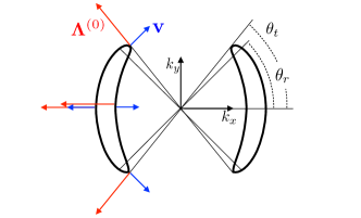
Figure 4: (Color online) Fermi surface of the model used to calculate the conductivity. Close to the transition, each reconstructed (banana-shaped) pocket mainly consists of two segments of circles with different radii. For the right pocket these segments are located at the polar angles $-\theta_{r}<\theta<\theta_{r}$. The turning regions, found in the range $\theta_{r}<\theta<\theta_{t}$ and equivalent ranges, are assumed to be much smaller than the main parts. The direction of the velocity (blue arrows) and the zero-field MFP (red arrows) are indicated for the left pocket.

 

IV.1 Mean free path

In the main part of the pocket, the velocity is parallel or antiparallel to the momentum, depending on the side of the pocket. Assuming the magnitude of the velocity to be constant at each side, we can write $\mathbf{v}_{\mathbf{k}}=v_{s}\,\hat{\mathbf{k}}$, where $\hat{\mathbf{k}}=\mathbf{k}/|\mathbf{k}|$ and $s=1,2$ denotes the side of the pocket. $v_{1}$ and $v_{2}$ have opposite sign. The zero-field MFP $\mathbf{\Lambda}^{(0)}_{\mathbf{k}}=\tau_{\mathbf{k}}\,(\mathbf{v}_{\mathbf{k}}+\mathbf{v}_{\bar{\mathbf{k}}})/2$, which is determined by the velocity averaged over the two sides, can then be written as $\mathbf{\Lambda}^{(0)}_{\mathbf{k}}=l\,\hat{\mathbf{k}}$, where $l=(v_{s}+v_{\bar{s}})/(2w_{i})$ and $\bar{s}=2,1$ if $s=1,2$.

In the turning region, the velocity direction changes by $180^{\circ}$ as we go along the pocket from $\theta_{r}$ over $\theta_{t}$ back to $\theta_{r}$. In contrast, the direction of the zero-field MFP is not reversed but only changes by $\pm 90^{\circ}$ on the way from $\theta_{r}$ to $\theta_{t}$ and then back by $\mp 90^{\circ}$ from $\theta_{t}$ to $\theta_{r}$. However, this result relies on the extreme assumption of $\delta$-function scattering. In reality, the peak in the scattering rate $W_{\mathbf{k}}^{\mathbf{k}^{\prime}}$ has a nonzero width $\delta k$, which results in $\mathbf{\Lambda}^{(0)}_{\mathbf{k}}$ being averaged over momentum-space regions of diameter $\delta k$. This naturally results in a smaller difference between the directions of $\mathbf{\Lambda}^{(0)}_{\mathbf{k}}$ at $\theta_{t}$ and $\theta_{r}$. If the size of the turning region is small compared to $\delta k$, the average is dominated by states from the large parts of the pockets. In agreement with our assumption of small turning regions, we thus neglect the variation of $\mathbf{\Lambda}^{(0)}_{\mathbf{k}}$ in the turning regions and assume the validity of $\mathbf{\Lambda}^{(0)}_{\mathbf{k}}=l\,\hat{\mathbf{k}}$ for the whole pocket.

We use Eq. (13) for the MFP $\mathbf{\Lambda}_{\mathbf{k}}$ in the presence of a magnetic field. We now divide the integral into a contribution from the main part and a contribution from the turning region,

$$\mathbf{\Lambda}_{\mathbf{k}} =\int_{\alpha}^{\alpha_{t}}\!\!d\alpha^{\prime}\,\mathbf{\Lambda}_{\mathbf{k}^{\prime}}^{(0)}\frac{1}{\tau_{\mathbf{k}^{\prime}}\,\omega_{\mathbf{k}^{\prime}}}\,\exp\bigg{(}{-}\int_{\alpha}^{\alpha^{\prime}}\!\!d\alpha^{\prime\prime}\frac{1}{\tau_{\mathbf{k}^{\prime\prime}}\,\omega_{\mathbf{k}^{\prime\prime}}}\bigg{)}$$ (16)

$$=\int_{\alpha}^{\alpha_{r}}\!\!d\alpha^{\prime}\,\mathbf{\Lambda}_{\mathbf{k}^{\prime}}^{(0)}\frac{1}{\tau\,\omega}\,\exp\bigg{(}{-}\frac{\alpha^{\prime}-\alpha}{\tau\,\omega}\bigg{)}+\exp\bigg{(}{-}\frac{\alpha_{r}-\alpha}{\tau\,\omega}\bigg{)}\,\int_{\alpha_{r}}^{\alpha_{t}}\!\!d\alpha^{\prime}\,\mathbf{\Lambda}_{\mathbf{k}^{\prime}}^{(0)}\frac{1}{\tau_{\mathbf{k}^{\prime}}\,\omega_{\mathbf{k}^{\prime}}}\,\exp\bigg{(}{-}\int_{\alpha_{r}}^{\alpha^{\prime}}\!\!d\alpha^{\prime\prime}\frac{1}{\tau_{\mathbf{k}^{\prime\prime}}\,\omega_{\mathbf{k}^{\prime\prime}}}\bigg{)},$$ (17)

where we have assumed a constant product of the relaxation time and the effective cyclotron frequency, $\tau_{\mathbf{k}}\,\omega_{\mathbf{k}}=\tau\,\omega$, in the main part of the pocket. To leading order in $|\theta_{r}-\theta_{t}|$, $\mathbf{\Lambda}_{\mathbf{k}^{\prime}}^{(0)}$ can be taken out of the second integral, which then reduces to unity, leading to the result

$$\mathbf{\Lambda}_{\mathbf{k}} = \int_{\alpha}^{\alpha_{r}}\!\!d\alpha^{\prime}\,\mathbf{\Lambda}_{\mathbf{k}^{\prime}}^{(0)}\frac{1}{\tau\,\omega}\,\exp\bigg{(}{-}\frac{\alpha^{\prime}-\alpha}{\tau\,\omega}\bigg{)}$$ (18)

$${}+\exp\bigg{(}{-}\frac{\alpha_{r}-\alpha}{\tau\,\omega}\bigg{)}\,\mathbf{\Lambda}_{\mathbf{k}_{r}}^{(0)}.$$

To calculate the $x$ and $y$ components of $\mathbf{\Lambda}_{\mathbf{k}}$ in a compact way, we introduce a complex notation and represent a vector $\mathbf{v}=(v^{x},v^{y})$ as $v^{x}+iv^{y}$. In this notation, the zero-field MFP, $\mathbf{\Lambda}^{(0)}_{\mathbf{k}}=l\,\hat{\mathbf{k}}$, can be written as $\Lambda_{\mathbf{k}}^{(0)x}+i\Lambda_{\mathbf{k}}^{(0)y}=l\,e^{i\theta}$. Inserting this into Eq. (18) we obtain

$$\Lambda_{\theta}^{x}+i\Lambda_{\theta}^{y} = \frac{l}{1+(\tau\,\omega)^{2}}\Big{[}e^{i\theta}(1+i\,\tau\,\omega)$$ (19)

$${}+\tau\,\omega\,e^{-(\theta_{r}-\theta)/\tau\,\omega}\,e^{i\theta_{r}}\big{(}\tau\,\omega-i\big{)}\Big{]},$$

where we use the polar angle $\theta$ as the parameter $\alpha$.

 

IV.2 Magnetoconductivity

The MFP in Eq. (19), together with the approximation $-n_{F}^{\prime}(\varepsilon_{\mathbf{k}})\approx\delta(\varepsilon_{\mathbf{k}})$, which is valid at low temperatures, determines the conductivity given in Eq. (14). As shown in Fig. 5, for small magnetic fields the magnetoconductivity is linear and highly anisotropic. Most strikingly, its sign depends on the direction of the electric field, which originates from the shift of weight of the distribution function in Eq. (13) towards the repulsive turning points, as discussed above.

The instability occurs when the effective cyclotron frequency is on the order of the inverse relaxation time, $1/\tau_{\mathrm{k}}$. For typical metals this corresponds to a magnetic-field strength on the order of $1\,\mathrm{T}$, which will be significantly enhanced for bad metals such as iron pnictides. Additional closed Fermi surfaces, which are not reconstructed and on which the orbital motion is not interrupted, add a positive contribution to the total conductivity. Although the instability should persist since the contribution from these pockets is strongly suppressed in large fields, the critical magnetic field will be further enhanced.

On the other hand, for small fields the additional contribution is only quadratic in $B$, and so the direction-dependent linear magnetoconductivity is unaffected. This makes it the most readily observable signature of the interrupted orbital motion.

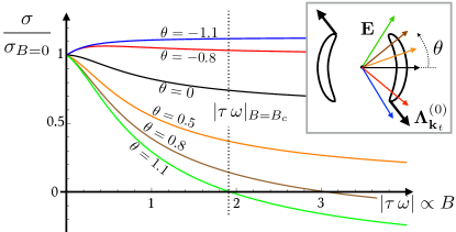
Figure 5: (Color online) Magnetoconductivity for various electric-field directions indicated in the inset. The model includes two reconstructed pockets with turning points at $\theta=\pm\pi/3,\pi\pm\pi/3$. $|\tau_{\mathbf{k}}\omega_{\mathbf{k}}|$ is set to $|\tau\,\omega|$ in the main parts of the reconstructed pockets. The turning regions are assumed to be small. The zero-field MFP, $\mathbf{\Lambda}^{(0)}_{\mathbf{k}}$, is taken to be parallel to the radial vector with constant absolute value.

 

V Four-pocket model

Besides the two-pocket scenario, the density-wave transition might also lead to four reconstructed pockets—one pair of symmetry-related electron-like pockets and one pair of symmetry-related hole-like pockets. The electron and hole pockets are generically different in size, where the relative size can be tuned, e.g., by doping and pressure. The calculation of the conductivity contribution of two additional pockets is analogous to the previous section. For simplicity, we take the absolute value of the velocity, the effective cyclotron frequency, and the absolute value of the zero-field MFP to be equal for all pockets.

The most important parameters in the four-pocket case are the relative size of the two inequivalent pocket pairs and the difference between their densities of states. As sketched in the inset of Fig. 6, we parametrize the two pocket sizes by the two extremal polar angles $\theta_{t,1}$ and $\theta_{t,2}$. The sketch also shows the gap between the two pockets, described by the angle $\Delta$. We will only consider small values for $\Delta$ as we expect to find interrupted orbital motion close to the transition temperature, where it is small.

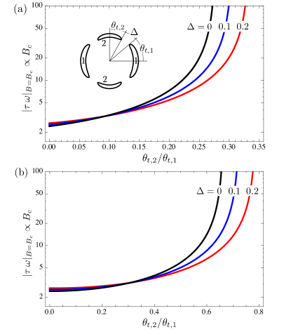
Figure 6: (Color online) Effective cyclotron frequency multiplied by the relaxation time, $|\tau\,\omega|_{B=B_{c}}$, as a function of the relative size of the pockets, $\theta_{t,2}/\theta_{t,1}$, for various gaps $\Delta$ between the pockets. $|\tau\,\omega|_{B=B_{c}}$ is a measure for the critical magnetic field, which is proportional to this quantity. (a) Results for equal densities of states of all pockets. The inset shows a sketch of the Fermi surface with the relevant parameters. (b) Results for the density of states of the first pair of pockets (pair 1) being four times larger then that of pair 2. Note the different scale of the $\theta_{t,2}/\theta_{t,1}$-axis.

The instability of the density-wave state is the most interesting consequence of interrupted orbital motion. As shown in Fig. 5, in the two-pocket model the instability occurs at magnetic fields for which the cyclotron frequency is on the order of the inverse relaxation time, $|\tau\,\omega|_{B=B_{c}}\sim 1$. In the following, we consider how the critical magnetic field is modified by the two additional pockets. In Fig. 6, we plot $|\tau\,\omega|_{B=B_{c}}\propto B_{c}$ for the four-pocket case as a function of the relative size of the pockets, for several values of $\Delta$. The results show, first of all, that a finite critical field $B_{c}$ still exists, i.e., the instability also occurs in the case of four pockets. Compared to the two-pocket case, the addition of two more pockets changes $B_{c}$ only slightly, as long as one pair of pockets is dominant: If the pockets have the same density of states, one pair should be larger by approximately a factor of $5$, whereas if it has a four times larger density of states, it must be only twice as large. If the pockets become close in size the critical field increases rapidly and the instability eventually vanishes.

Qualitatively, this behavior can be understood from the conductivity in the limit of strong magnetic fields. The obvious extension of Eq. (15) to the four-pocket case is

$$\sigma = 2e^{2}\,\big{[}D_{1}(E_{F})\,(\bar{\mathbf{v}}_{1}\cdot\hat{\mathbf{E}})\,\big{(}\mathbf{\Lambda}^{(0)}_{t,1}\cdot\hat{\mathbf{E}}\big{)}$$ (20)

$${}+D_{2}(E_{F})\,(\bar{\mathbf{v}}_{2}\cdot\hat{\mathbf{E}})\,\big{(}\mathbf{\Lambda}^{(0)}_{t,2}\cdot\hat{\mathbf{E}}\big{)}\big{]}.$$

According to the discussion in section III, the contribution of each pair is negative for certain directions $\hat{\mathbf{E}}$ of the electric field. These directions are indicated in Fig. 7. Here, we assume the effective cyclotron motion to be in the same direction, namely counterclockwise, for the electron-like and the hole-like pockets. This is because the effective cyclotron frequency is the difference between the bare cyclotron frequencies for the two states $|\mathbf{k}\rangle$ and $|\bar{\mathbf{k}}\rangle$, which are proportional to the inverse effective masses. It is natural to assume that either the hole or the electron band in the disordered state has the larger effective mass for all $\mathbf{k}$. This means that the effective cyclotron frequency has the same sign for both types of reconstructed pockets. Furthermore, the vector MFP at the turning points of both the electron-like and the hole-like pockets is assumed to point outward. The direction of the MFP is determined by the vector sum of velocities of the two states $|\mathbf{k}\rangle$ and $|\bar{\mathbf{k}}\rangle$, i.e., set by the larger velocity. It is again natural to assume that either the hole or the electron band in the disordered state has the larger Fermi velocity so that for both types of reconstructed pockets the MFP will point either parallel or antiparallel to the radial direction. Whether we choose parallel or antiparallel does not matter for the conductivity as the sign drops out. We observe that one of the two terms in Eq. (20) is always positive. This positive term can raise the conductivity to positive values, which explains why the instability can be absent in the four-pocket case. However, if one pocket becomes larger than the other the spacing between the regions of negative contributions becomes smaller. Then directions exist for which the contribution from the larger pockets is negative [region 1 in Fig. 7(b)], while the one from the smaller pockets is positive but smaller in magnitude since its sign change is close by, resulting in a negative total conductivity. This tendency is further enhanced if the larger pocket has a larger density of states, which increases the negative contribution.

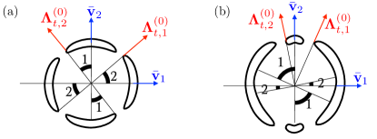
Figure 7: (Color online) Angle ranges of the electric-field direction $\hat{\mathbf{E}}$, for which the first term (1) and the second term (2) in Eq. (20) are negative for the case that (a) the pairs of pockets are nearly of the same size and (b) one pair of pockets is significantly larger than the other. In the second case, the two negative regions come closer to each other, which favors negative total conductivity.

The magnetoconductivity for the four-pocket case, shown in Fig. 8(a), is qualitatively similar to the two-pocket case (cf. Fig. 5). Figure 8(b) shows the differential magnetoconductivity at $B=0$. Note that the linear contribution at low fields, the sign of which depends on the electric-field direction, persists also for systems in which one pair of pockets dominates only weakly over the other. Although no instability occurs in this case, the direction dependence of the linear contribution can still serve as a signature of interrupted orbital motion.

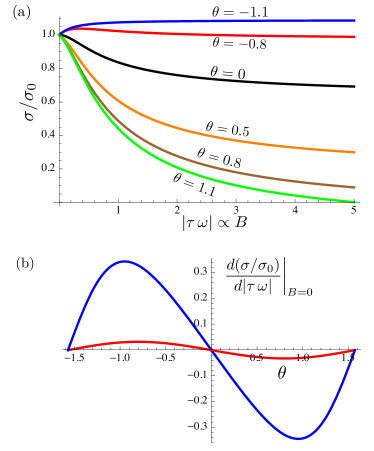
Figure 8: (Color online) (a) Magnetoconductivity for various electric-field directions, $D_{1}(E_{F})=4\,D_{2}(E_{F})$, $\Delta=0.1$, and $\theta_{t,2}/\theta_{t,1}=0.5$. (b) Differential magnetoconductivity at $B=0$ as a function of the electric-field direction for $D_{1}(E_{F})=4\,D_{2}(E_{F})$ (blue curve) and $D_{1}(E_{F})=D_{2}(E_{F})$ (red curve). In both cases, $\Delta=0.1$ and $\theta_{t,2}/\theta_{t,1}=0.5$. Note that for $D_{1}(E_{F})=D_{2}(E_{F})$ (red curve), one pair of pockets dominates only weakly over the other so that no instability occurs, while the sign-changing linear magnetoconductivity is still present.

 

VI Conclusions

In summary, we have investigated the magnetotransport properties in a metal close to a density-wave instability. We find that strongly anisotropic scattering between approximately nested Fermi pockets can lead to reversed orbital motion of charge carriers in a magnetic field. In the density-wave state, this generically results in points on the Fermi surface where the orbital motion changes direction.

The interruption of the orbital motion gives rise to linear magnetoconductivity, the sign of which depends on the direction of the applied electric field, and an unusual instability of the system characterized by a vanishing longitudinal conductivity in strong magnetic fields. The latter effect, which leads to a so-far unexplored inhomogeneous state, might be hard to access experimentally if the system contains additional charge carriers with uninterrupted orbital motion, such as in iron pnictides. More promising candidate materials are excitonic systems without additional Fermi surfaces besides the nearly nested ones. The effect of sign-changing linear magnetoconductivity, on the other hand, does not require strong fields and is not overshadowed by the contribution of additional Fermi surfaces, which is quadratic in the magnetic field. We expect this effect to be visible in the direction-resolved magnetoresistance in weak magnetic fields.