Semiclassical limit of the focusing NLS: Whitham equations and the Riemann-Hilbert Problem approach

Abstract.

The main goal of this paper is to put together: a) the Whitham theory applicable to slowly modulated $N$-phase nonlinear wave solutions to the focusing nonlinear Schrödinger (fNLS) equation, and b) the Riemann-Hilbert Problem approach to particular solutions of the fNLS in the semiclassical (small dispersion) limit that develop slowly modulated $N$-phase nonlinear wave in the process of evolution. Both approaches have their own merits and limitations. Understanding of the interrelations between them could prove beneficial for a broad range of problems involving the semiclassical fNLS.

1. Introduction

In this paper we consider the focusing Nonlinear Schrödinger (fNLS) equation

(1.1) $$i\varepsilon\partial_{t}\psi+\frac{1}{2}\varepsilon^{2}\partial_{x}^{2}\psi+|\psi|^{2}\psi=0,$$

where $x\in{\mathbb{R}}$ and $t\geq 0$ are space-time variable and $\varepsilon>0$. In the semiclassical (small dispersion) limit we take $\varepsilon\rightarrow 0^{+}$. The fNLS is a basic model for self-focusing and self-modulation, for example, it governs nonlinear transmission of light in optical fibers; it can also be derived as a modulation equation for a broad class of nonlinear systems. It was first integrated (with $\varepsilon=1$) by Zakharov and Shabat [38], who produced a Lax pair for it and used the inverse scattering procedure to describe the time evolution of general decaying potentials ($\lim_{|x|\to\infty}\psi(x,0,\varepsilon)=0$) in terms of the scattering data, that is, radiation and solitons.

Integrability of the fNLS enables the existence of the finite-gap solutions, the non-decaying quasi-periodic potentials with many remarkable properties [1]. Slow modulations of these potentials are described by the Whitham modulation equations [37], a system of quasilinear equations derived by the averaging procedure applied to fNLS. The remarkable feature of the fNLS evolution is that the modulated finite-gap potentials arise as asymptotic solutions in the initial value problems for the fNLS with non-oscillating initial conditions (e.g. Gaussian or sech initial data for (1.1)). This has been understood in the framework of the Riemann-Hilbert problem (RHP) approach to the inverse scattering yielding both the finite-gap potentials and their modulations within the rigorous asymptotic description of the semiclassical fNLS evolution. However, the connections between the Whitham modulation theory and the RHP approach have not been properly traced.

The main results of the present paper:

• We link the main objects of the Whitham theory (Riemann invariants, their characteristic velocities, fundamental differentials $dp,dq$) with the corresponding objects coming from the RHP approach, which are expressed in terms of the $g$-function from the RHP approach and the corresponding hyperelliptic Riemann surface $\mathcal{R}$;

• We derive several equivalent forms of the modulation equations (by which we mean systems of transcendental equations for the branchpoints of $\mathcal{R}$), and use them to show that various forms of the generalized hodograph solutions of the Whitham equations are satisfied;

• we use the $g$-function to establish the role of the potential for the differentials $dp,dq$ in determining the breaking (phase transition) curves and double point velocities for the fNLS.

The first (spatial) equation of the Lax pair for the fNLS is known as Zakharov - Shabat (ZS) system

(1.2) $$i\varepsilon\frac{d}{dx}W=\begin{pmatrix}z&\psi\\ \bar{\psi}&-z\end{pmatrix}W~{},$$

where $z$ is a spectral parameter and $W$ is a $2$ by $2$ matrix-function.

The scattering data, corresponding to the initial data $\psi(x,0,\varepsilon)$, consist of the reflection coefficient $r_{0}(z,\varepsilon)$, as well as of the points of the discrete spectrum, if any, together with their norming constants. The time evolution of the scattering data is simple ([38]). The corresponding evolution of a given potential is obtained through the inverse scattering transformation (IST) of the evolving scattering data. The inverse scattering transform for the fNLS equation (1.1) at the point $x,t$ can be cast as the following matrix Riemann-Hilbert Problem (RHP) in the spectral $z$-plane: find a $2\times 2$ matrix-valued function $m(z)=m(z;x,t,\varepsilon)$, which depends on the asymptotic parameter $\varepsilon$ and the external parameters $x,t$, such that: i) $m(z)$ is analytic in ${\mathbb{C}}\backslash\Gamma$, where the contour $\Gamma={\mathbb{R}}$ has the natural orientation; ii)

(1.3) $$m_{+}=m_{-}\begin{pmatrix}1+r\bar{r}&\bar{r}\cr r&1\cr\end{pmatrix}=m_{-}V~{}$$

on the contour $\Gamma$, where $r(z,\varepsilon)=r_{0}(z,\varepsilon)\exp[{2i\over\varepsilon}(2z^{2}t+zx)]$ and $m_{\pm}(z)=\lim_{\delta\rightarrow 0}m(z\pm i\delta)$ with $\delta>0$ and $z\in{\mathbb{R}}$; iii) $\lim_{z\rightarrow\infty}m(z)={\bf 1},$ where ${\bf 1}$ denotes the identity matrix. In the presence of solitons the contour $\Gamma$ contains additional small circles around the eigenvalues with the corresponding jump-matrices (see, for example, [30] or [19]).

A complementary approach to the analysis of nonlinear dispersive equations is provided by the Whitham modulation theory which produces a system of quasilinear partial differential equations governing slow modulations of periodic or quasi-periodic waves. A prominent area where the Whitham method proved extremely useful is the theory of dispersive shock waves (DSWs) [16], [11]

We consider an $N$-phase quasi-periodic solution of the fNLS equation (1.1),

(1.4) $$\psi=\psi_{N}(\varepsilon^{-1}\eta_{1},\varepsilon^{-1}\eta_{2},\dots,\varepsilon^{-1}\eta_{N};{\boldsymbol{\alpha}},\bar{\boldsymbol{\alpha}}),\quad\hbox{where}\quad\eta_{j}=k_{j}x+\omega_{j}t+\eta^{0}_{j}.$$

Here $\boldsymbol{\alpha}\equiv\{\alpha_{j}\}_{j=0}^{N}\in\mathbb{C}^{N}$ and c.c. are the branchpoints of the hyperelliptic Riemann surface of genus $N$ on which (1.4) lives [1], the (normalized by $\varepsilon$) wavenumbers $k_{j}$ and the frequencies $\omega_{j}$ are defined in terms of the branchpoints, and $\eta_{j}^{0}$ are arbitrary initial phases. Now, if the parameters $\alpha_{j}$, $\bar{\alpha}_{j}$ are allowed to vary slowly in space and time they must satisfy the Whitham modulation equations,

(1.5) $$(\alpha_{j})_{t}=V_{j}^{(N)}({\boldsymbol{\alpha}},\boldsymbol{\bar{\alpha}})(\alpha_{j})_{x},\quad(\bar{\alpha}_{j})_{t}=\overline{V}_{j}^{(N)}(\boldsymbol{\alpha},\boldsymbol{\bar{\alpha}})(\bar{\alpha}_{j})_{x},\qquad j=0,\dots,N\,,$$

so that $\alpha_{j}$, $\bar{\alpha}_{j}$ are Riemann invariants. The characteristic velocities $V_{j}^{(N)}$, $\overline{V}_{j}^{(N)}$ are expressed in terms of the Riemann invariants $\alpha_{j}$ through hyperelliptic (for $N\geq 2$) or complete elliptic (for $N=1$) integrals. For $N=0$ the Whitham system (1.5) has the form

(1.6) $$(\alpha_{0})_{t}=(\tfrac{3}{2}\alpha_{0}+\tfrac{1}{2}\bar{\alpha}_{0})(\alpha_{0})_{x},\qquad(\bar{\alpha}_{0})_{t}=(\tfrac{3}{2}\bar{\alpha}_{0}+\tfrac{1}{2}\alpha_{0})(\bar{\alpha}_{0})_{x}\,,$$

and is equivalent to the dispersionless limit of (1.1)

(1.7) $$\rho_{t}+(\rho u)_{x}=0,\quad u_{t}+uu_{x}-\rho_{x}=0\,,$$

where the Riemann invariants and characteristic speeds in (1.6) are expressed in terms of the hydrodynamic “density” $\rho=|\psi|^{2}\geq 0$ and “velocity” $u=-i\varepsilon^{-1}(\arg\psi)_{x}$ as

(1.8) $$\alpha_{0}=-(\frac{u}{2}+i\sqrt{\rho}),\qquad V_{0}^{(0)}=\tfrac{3}{2}\alpha_{0}+\tfrac{1}{2}\bar{\alpha}_{0}=-(u+i\sqrt{\rho})\,.$$

One can see that the characteristics of (1.7) are complex unless $\rho=0$ implying nonlinear modulational instability of the NLS equation (1.1) in the long-wave limit, and hence, ill-posedness of the initial-value problem for (1.6) for all but analytical initial data.

For $N\geq 1$ the characteristic velocities $V_{j}^{(N)}$ in (1.5) are also complex, however, vanishing of the imaginary parts for some $V_{j}$’s is possible. This “partial hyperbolicity” property makes the Whitham systems for $N\geq 1$ radically different compared to the genus zero case and has major implications in terms of stability of some solutions [10].

There are (at least) two ways of looking at the Whitham equations. Originally, they were introduced in [35] as the equations obtained by the averaging of dispersive conservation laws over the family of periodic or quasi-periodic solutions. Later, Whitham put his method in the very general variational principle framework [36]. Another approach leading to the same set of equations is the multiple-scale (nonlinear WKB) expansions method [24]. If the original dispersive equation is IST integrable, the associated Whitham system turns out to be also integrable in the sense which will be explained later on.

Using the finite-gap theory of the KdV equation [26], [21] Flaschka, Forest and McLaughlin [14] showed that the endpoints of the spectral bands of quasi-periodic finite-gap potentials of the quantum-mechanical Schrödinger operator are Riemann invariants of the Whitham modulation system associated with the KdV equation. Analogous result for the fNLS equation was obtained by Forest and Lee [15] and Pavlov [27].

The second context in which the Whitham equations appear is due to Lax, Levermore and Venakides [22], [33], [23] who derived them as the equations governing the zero dispersion limit of the KdV equation. The dispersion parameter $\varepsilon$ determines the typical scale of nonlinear oscillations in the KdV solution so the limit as $\varepsilon\to 0$ exists only in a weak sense. Venakides provided the bridge between the Flaschka-Forest-McLaughlin (wave packet averages) and Lax-Levermore (weak limits) results by developing the higher-order Lax-Levermore theory [34]. Finally, the all-encompassing approach to the small-dispersion KdV was developed by Deift, Venakides and Zhou [5], who introduced the nonlinear steepest descent method for the RHP associated with the (semi-classical) inverse scattering problem.

The Whitham equations naturally arise in the RHP construction as the equations governing the evolution of the spectral branch points $\alpha_{j}$, $\bar{\alpha}_{j}$. To be precise, the RHP theory yields the hodograph solution to the Whitham equations as the combination of the moment conditions and the Boutroux conditions. Although the connection of the Whitham equations with the RHP construction of the semi-classical limit is generally well known it has not been explored to any depth for the fNLS equation. The apparent reason for such an omission is twofold: (i) the existing rigorous analyses of the IVPs for the fNLS equation (see [19], [30] and references therein), performed within the RHP framework, already contain all the information about slow modulations of the solution so there is no need to recover it with the aid of a more restricted Whitham approach; (ii) the Whitham equations (1.5) are elliptic so their application to the problems outside the firmly established facts of the existence and convergence of the relevant solution was suspect. Nevertheless, the success of the application of the Whitham theory to dispersively modified hyperbolic conservation laws, particularly in the DSW theory for the KdV and defocusing NLS equations (see [11] and references therein), provides a strong incentive for the development of a similar theory for the elliptic, focusing case, which is also supported by the extensive numerical evidence that the key features of the small-dispersion “hyperbolic” nonlinear dynamics, such as the co-existence of smooth and rapidly oscillating regions and weak convergence, hold true for at least some cases of the semi-classical fNLS evolution (see, e.g., [3], [4], [10]).

The modulation theory approach to the description of the small dispersion limit of integrable “hyperbolic” equations, such as KdV or defocusing NLS, involves solution of a nonlinear free boundary problem for the associated Whitham modulation system via the so-called matching regularization procedure. This procedure represents an extension of the original Gurevich-Pitaevskii method of the modulation description of a DSW in the KdV equation [13] and prescribes the solution genus increase every time it undergoes a gradient catastrophe. The modulation solutions of different genera are “glued” in a spectial way along the breaking curves which are free boundaries and whose determination is part of the solution (see e.g. [12] for the detailed description of the matching regularization procedure for the KdV equation with monotone initial conditions).

The matching regularization procedure can be relatively easily implemented in the problems involving the fNLS solutions with $N=0$ and $N=1$. This was done in [7], [20], [10] for the fNLS dam-break problem. The modulation solution of [7], [20] was rigorously confirmed in [17] within the RHP analysis of the semi-classical fNLS with the square barrier initial data. The breaks involving $N\geq 2$ as in the first break for the sech potential ([19], [30]), or any higher breaks have not been considered within the Whitham theory with the only exception [10], where the modulation solution beyond the second break was used to predict the generation of rogue waves (note, however, that the second break was considered in [25] in the framework of the RHP approach).

The above discussion strongly suggests that it would be highly desirable to develop a method for solving the fNLS-Whitham equations in problems involving formation of oscillatory regions characterized by the genus $N\geq 2$. It is also clear that the RHP analysis, in particular, the nonlinear steepest descent method with the $g$-function mechanism, can provide valuable clues to the structure of the modulation solutions. Indeed, certain elements of the RHP approach offer an elegant way to circumvent the matching regularization procedure which could be quite awkward when matching modulation solutions with $N\geq 2$. Thus, a closer exploration of the interconnections between the RHP theory of the small-dispersion fNLS limit and the counterpart Whitham modulation theory seems a worthwhile task. Indeed, an appropriate combination of the Whitham theory and some key elements of the RHP which could be termed a “formal RHP analysis”, complemented by careful numerical simulations recently proved very effective for solving problems of immediate physical interest [10].

The paper is organized as follows. In Sections 2, 3 we present the general Whitham theory approach and the RHP approach respectively, as applied to semiclassical fNLS. These two approaches are compared in the case of genus zero in Section 4. In Section 5 we derive an explicit expression for the $g$-function (in the determinantal form) in higher genera regions for the box-type potentials and discuss its connections with the corresponding hyperelliptic Riemann surface $\mathcal{R}$. Solutions of the Whitham equations in terms of $g$-function are discussed in Section 6. The results of this section are based on Theorem 6.1 about three equivalent forms of modulation equations. The results of Sections 5, 6 in the case of analytic potentials were discussed in Section 7. Transitions between the regions of different genera and the characteristic velocities along breaking curves are discussed in Section 8. In particular, we show that, in the square barrier (“box”) potential case, a pair of collided branchpoints on the breaking curve always has real characteristic velocity.

2. Whitham equations and hodograph solution

The Whitham equations for the fNLS 1.1 can be represented as a single generating conservation equation [15], [27]

(2.1) $$\partial_{t}dp=\partial_{x}dq,$$

where $dp(z,\alpha,\bar{\alpha})$ and $dq(z,\alpha,\bar{\alpha})$ are certain meromorphic differentials of the second kind (the quasimomentum and the quasienergy) on the hyperlliptic Riemann surface $\mathcal{R}$ of genus $N$ defined by the radical $R(z)=\sqrt{\prod_{j=0}^{N}(z-\alpha_{j})(z-\bar{\alpha}_{j})}$ where $z$ is the complex spectral parameter. The branch points $\boldsymbol{\alpha}=(\alpha_{0},\dots,\alpha_{N})$ and c.c. are the points of simple spectrum of the periodic Zakharov-Shabat operator (1.2).

The quasimomentum and quasienergy differentials $dp$ and $dq$ are uniquely defined by the following properties [15]:

(a) $dp$ and $dq$ have the poles of order two and three respectively at $\infty^{\pm}$ on $\mathcal{R}$ and no other poles;

(b) the expansions of $dp$ and $dq$ in the local coordinate $z=\zeta^{-1}$ near $\infty^{\pm}$ are

(2.2) $$\begin{split}dp\sim\pm[-\frac{1}{\zeta^{2}}+\hbox{holomorphic part}]\ \hbox{near}\ \infty^{\pm},\\ dq\sim\pm[-\frac{2}{\zeta^{3}}+\hbox{holomorphic part}]\ \hbox{near}\ \infty^{\pm}\end{split}$$

(c) $dp$ and $dq$ satisfy the normalization conditions

(2.3) $$\oint\limits_{\hat{\gamma}_{j}}dp=\oint\limits_{\hat{\gamma}_{j}}dq=0\,,\qquad j=1,\dots,N,$$

where $\hat{\gamma}_{j}$ is a clockwise loop around the branchcut connecting $\alpha_{j}$ and $\bar{\alpha}_{j}$ (the $\mathbf{A}$-cycle).

Note that $dp,dq$ are Schwarz symmetrical differentials, so that normalization conditions (2.3) are equivalent to Boutroux normalization conditions for $dp,dq$: all the cycles of $dp,dq$ on $\mathcal{R}$ are real.

The integrals over the $\mathbf{B}$-cycles, canonically conjugated to the $\mathbf{A}$-cycles, give the fundamental wavenumbers $k_{j}$ and frequencies $\omega_{j}$:

(2.4) $$k_{j}=\oint\limits_{\mathbf{B_{j}}}dp\,,\quad\omega_{j}=\oint\limits_{\mathbf{B_{j}}}dq\,.$$

An alternative useful representation for the wave numbers and frequencies in terms of holomorphic differentials is:

(2.5) $$k_{j}=-4\pi i\varkappa_{N,j}\,,\qquad\omega_{j}=-4\pi i\left[\tfrac{1}{2}\sum\limits_{k=0}^{N}(\alpha_{k}+\bar{\alpha}_{k})\ \varkappa_{N,j}+\varkappa_{N-1,j}\right],\quad j=1,\dots,N,$$

where $\varkappa_{j,k}(\boldsymbol{\alpha},\boldsymbol{\bar{\alpha}})$ are the coefficients of the normalized holomorphic differentials found from the system

(2.6) $$\sum\limits_{i=1}^{N}\varkappa_{m,k}\oint\limits_{\hat{\gamma}_{k}}\frac{z^{m}}{R(z)}dz=\delta_{mk}\,,\quad m,k=1,\dots,N.$$

Here $\delta_{mk}$ is the Kronecker symbol.

The generating equation (2.1) has several fundamental consequences:

(i) By multiplying (2.1) by $(z-\alpha)^{3/2}$ and letting $z\to\alpha_{j}$ one obtains the diagonal system (1.5) with the characteristic speeds $V_{j}$ given by

(2.7) $$V_{j}=\frac{dq}{dp}{\bigg{|}}_{z=\alpha_{j}},\quad\overline{V}_{j}=\frac{dq}{dp}{\bigg{|}}_{z=\bar{\alpha}_{j}}.$$

(ii) By expanding (1.5) near $z=\infty$ we obtain an infinite series of averaged local conservation laws of the form $\partial_{t}P_{j}({\boldsymbol{\alpha}},{\boldsymbol{\bar{\alpha}}})=\partial_{x}Q_{j}({\boldsymbol{\alpha}},{\boldsymbol{\bar{\alpha}}})$, where $P_{j}$ are the averaged densities of the NLS conservation laws and $Q_{j}$ the corresponding averaged fluxes. Any $2N+2$ of these conservation laws are independent.

(iii) By integrating (1.5) over each of the $N$ $\mathbf{B}$-cycles we obtain, on using (2.4), $N$ equations for conservation of waves

(2.8) $$\frac{\partial}{\partial t}k_{j}(\boldsymbol{\alpha},\boldsymbol{\bar{\alpha}})=\frac{\partial}{\partial x}\omega_{j}(\boldsymbol{\alpha},\boldsymbol{\bar{\alpha}}),\qquad j=1,\dots,N\,.$$

Since (2.8) must be consistent with (1.5) we obtain a compact and physically insightful representations for $V_{j}$’s as nonlinear group velocities is (see [8], [9], [11]).

(2.9) $$V_{j}^{(N)}=\frac{\partial\omega_{i}}{\partial\alpha_{j}}/\frac{\partial k_{i}}{\partial\alpha_{j}},\qquad\hbox{for any}\quad i=1,\dots,N.$$

We note that equations (2.8) represent the consistency conditions in the formal averaging procedure [36, 37] as well as in the the WKB-type multiple-scale expansions [24], [37], [6] leading to the same Whitham system (1.5). Within this (general) modulation theory framework the wavenumbera $k_{j}$ and the frequences $\omega_{j}$ in the modulated wave are defined as the derivatives of the phase $\eta_{j}$:

(2.10) $$k_{j}=(\eta_{j})_{x},\quad\omega_{j}=(\eta_{j})_{t},\quad j=1,\dots,N.$$

Clearly, the definitions (2.10) by Clairaut’s theorem are consistent with the wave conservation equation (2.8).

The Whitham system (1.5) can be integrated using the Tsarev generalized hodograph transform [32]. This method was originally developed for hyperbolic systems of hydrodynamic type but is equally applicable to elliptic systems. Tsarev’s result in the application to our present problem can be formulated as follows. Any local non-constant solution of the modulation system (1.5) for a given genus $N$ is given in an implicit form by the system of $N$ algebraic equations with complex coefficients

(2.11) $$x+V_{j}(\boldsymbol{\alpha},\boldsymbol{\bar{\alpha}})t=w_{j}(\boldsymbol{\alpha},\boldsymbol{\bar{\alpha}}),\quad x+\overline{V}_{j}(\boldsymbol{\alpha},\boldsymbol{\bar{\alpha}})t=\bar{w}_{j}(\boldsymbol{\alpha},\boldsymbol{\bar{\alpha}}),\qquad j=1,2,\dots,N,$$

where the characteristic speeds $V_{j}(\boldsymbol{\alpha},\boldsymbol{\bar{\alpha}})\equiv V^{(N)}_{j}(\boldsymbol{\alpha},\boldsymbol{\bar{\alpha}})$ are given by (2.9), (2.5). The $2N$ unknown complex functions $w_{j}$, $\bar{w}_{j}$, $j=1,2,\dots,N$ satisfy the system of linear partial differential equations

(2.12) $$\frac{\partial_{\alpha_{j}}w_{k}}{w_{k}-w_{j}}=\frac{\partial_{\alpha_{j}}V_{k}}{V_{k}-V_{j}}\quad\hbox{and \ c.c.};\quad j,k=1,2,\dots,N,\quad k\neq j\,,$$

where $\partial_{\alpha_{j}}\equiv\frac{\partial}{\partial\alpha_{j}}$. System (2.12) is overdetermined but compatible for the NLS case studied here owing to the integrability of fNLS being preserved under the Whitham averaging [6].

We now note that, for the solution $q(x,t;\varepsilon)$ of the semi-classical fNLS to have an asymptotic representation in the form of the modulated finite-band potential locally depending on $N$ “torus” phases $\varepsilon^{-1}\eta_{j}=\varepsilon^{-1}(k_{j}x+\omega_{j}t+\eta_{j}^{0})$ (see (1.4)), and at the same time to satisfy the general kinematic conditions (2.10) one must require that the “initial phases” $\eta_{j}^{0}$ are not constants but depend on $x,t$ via the branch points $\boldsymbol{\alpha},\boldsymbol{\bar{\alpha}}$. To this end we introduce the modulation phase shift functions $\Upsilon_{j}(\boldsymbol{\alpha,\bar{\alpha}})$ by $\eta_{j}^{0}=-\Upsilon_{j}(\boldsymbol{\alpha,\bar{\alpha}})$ so that the normalized phases $\eta_{j}$ assume the form (see [10], [11])

(2.13) $$\eta_{j}=k_{j}x+\omega_{j}t-\Upsilon_{j}(\boldsymbol{\alpha},\boldsymbol{\bar{\alpha}}).$$

Then the definition of the local wavenumber in (2.10) implies

(2.14) $$k_{j}=\frac{\partial(k_{j}x+\omega_{j}t-\Upsilon_{j})}{\partial x},\quad j=1,2,$$

which yields

(2.15) $$\frac{\partial k_{j}}{\partial\alpha_{m}}x+\frac{\partial\omega_{j}}{\partial\alpha_{m}}t=\frac{\partial\Upsilon_{j}}{\partial\alpha_{m}}\,,\quad\hbox{and c.c.},\quad j,m=1,2,\dots,N.$$

provided $\partial\alpha_{j}/\partial x\neq 0$, $\partial\bar{\alpha}_{j}/\partial x\neq 0$, $j=1,2$. Here $k_{j}({\boldsymbol{\alpha}},{\boldsymbol{\bar{\alpha}}})$ and $\omega_{j}(\boldsymbol{\alpha},\boldsymbol{\bar{\alpha}})$ are defined by (2.5), and $\Upsilon_{j}$’s are yet to be found. Note that the second condition (2.10) leads to the same set of equations (2.15). As we shall see, only half of the equations (2.15) are independent, so it is sufficient to consider either $j=1$ or $j=2$. We also note that equations (2.15) admit a compact and elegant representation in the form of the stationary phase conditions:

(2.16) $$\frac{\partial\eta_{j}}{\partial\alpha_{m}}=0,\qquad\frac{\partial\eta_{j}}{\partial\bar{\alpha}_{m}}=0,\quad j,m=1,2,\dots,N.$$

For given functions $\Upsilon_{j}(\boldsymbol{\alpha},\boldsymbol{\bar{\alpha}})$ equations (2.15) fully define the modulations $\boldsymbol{\alpha}(x,t)$, $\boldsymbol{\bar{\alpha}}(x,t)$ (assuming invertibility of (2.15), which is not guaranteed a priori). Comparing equations (2.15) with the hodograph solution (2.11) and using the representation (2.9) for the characteristic speeds $V_{j}(\boldsymbol{\alpha},\boldsymbol{\bar{\alpha}})$ in (2.11) one readily makes the identification

(2.17) $$w_{m}=\frac{\partial_{\alpha_{m}}\Upsilon_{j}}{\partial_{\alpha_{m}}k_{j}}\quad\hbox{and c.c.},\quad j,m=1,2,\dots,N\,.$$

Now we observe that formula (2.17) must yield the same function $w_{m}(\boldsymbol{\alpha},\boldsymbol{\bar{\alpha}})$ for all values of $j$. This is a consequence of the consistency of the genus $N$ Whitham modulation system with $N$ “extra” conservation laws (2.8) (the same argument was used to establish the ‘nonlinear group velocity’ representation (2.9) for the characteristic speeds of the Whitham modulation system). Thus, it is sufficient to consider any $N$ of the equations (2.15) for any given $j$.

Summarizing, the integration of the Whitham equations reduces to the determination of the “modulation phase shift” vector function $\boldsymbol{\Upsilon}(\boldsymbol{\alpha},\boldsymbol{\bar{\alpha}})$. As we shall see, this function naturally arises in the RHP construction, thus enabling one to circumvent the complicated matching regularization procedure necessary for the determination of the dependence of $\boldsymbol{\Upsilon}(\boldsymbol{\alpha},\boldsymbol{\bar{\alpha}})$ on the fNLS initial conditions within the Whitham modulation theory framework. Another feature of the RHP analysis enhancing the modulation theory is that it reveals the precise mechanism of the genus change across a breaking curve. We note that within the Whitham modulation theory the genus change determination is essentially an “educated guess” process which must be confirmed by the construction of the full modulation solution.

3. RHP approach to the inverse scattering for the fNLS. The $g$-function.

It is well known (see, for example [39]) that the RHP (1.3) has a unique solution $m(z)$ that has asymptotics $m(z)={\bf 1}+{m_{1}\over z}+O(z^{-2})$ as $z\rightarrow\infty$, and that the solution to the NLS (1.1) is given by $\psi(x,t,\varepsilon)=-2(m_{1})_{12}$, where $(m_{1})_{12}$ denotes the $(1,2)$ entry of matrix $m_{1}$. In the case when $r_{0}(z,\varepsilon)$ has analytic continuation into the upper halfplane, the RHP for $m(z)$ is simplified by factorizing the jump matrix

(3.1) $$V=\begin{pmatrix}1+r\bar{r}&\bar{r}\cr r&1\cr\end{pmatrix}=\begin{pmatrix}1&\bar{r}\\ 0&1\end{pmatrix}\begin{pmatrix}1&0\\ r&1\end{pmatrix}=V_{-}V_{+}~{}~{},$$

and, thus, “splitting” the jump condition (1.3) into two jumps: one with triangular jump matrix $V_{+}$ along some contour $\Gamma^{+}$ in the upper halfplane $\bar{\mathbb{C}}^{+}$ and the other with triangular jump matrix $V_{-}$ along some contour $\Gamma_{-}$ in the lower halfplane $\bar{\mathbb{C}}^{-}$ (here we assume that ${\mathbb{R}}$ is included in $\bar{\mathbb{C}}^{\pm}$). Contours $\Gamma^{\pm}$ are deformations of ${\mathbb{R}}$. Due to the Schwarz symmetry of the ZS problem, contours $\Gamma^{\pm}$ can be chosen to be symmetric to each other with respect to the real axis, and we can restrict our attention only to the contour $\Gamma^{+}\subset\bar{\mathbb{C}}^{+}$. For simplicity, we assume $\Gamma$ to be a simple, smooth (except for a finitely many points) contour without self-intersections.

The central idea of the Deift-Zhou nonlinear steepest descent method for asymptotic analysis of RHPs is proper factorization of a jump matrix accompanied by the proper deformation of the contour $\Gamma$. That is why we assumed that $r_{0}(z;\varepsilon)$ has analytic continuation from ${\mathbb{R}}$ into $\bar{\mathbb{C}}^{+}$. Another essential element in the nonlinear steepest descent analysis is the concept of $g$-function. We use the $g$-function $g(z)=g(z;x,t)$ to define a transformation, that reduces the RHP (1.3) to another RHP that, in the small $\varepsilon$ limit, has piece-wise constant (in $z$) jump matrices. In some sense, the $g$ function can be compared with the oscillatory phase function in the WKB method, which reduces a singularly perturbed ODE (like, for example, (1.2)) to a system that can be solved by a power series in the small parameter $\varepsilon$ (or a fractional power of $\varepsilon$).

The $g$ is build for a particular solution of the fNLS (1.1), given by the corresponding scattering data. Thus, the $g$ function will be defined by a Schwarz symmetric function $f_{0}(z)$, that can be associated with a scaled logarithm of $r_{0}(z)$. We assume $f_{0}(z)$ to be analytic, or at least, piece-wise analytic, in some Schwarz symmetrical domains that contain $\Gamma^{+}$ and $\Gamma^{-}$ respectively. The meaning of piece-wise analyticity will be addressed below.

Because of Schwarz symmetry, $f_{0}(z)$ may have a purely imaginary jump $2i\Im f_{0}$ on ${\mathbb{R}}$. Depending on whether or not $\Im f_{0}(z)\equiv 0$ on some interval of ${\mathbb{R}}$, $f_{0}(z)$ may have either one or two analytic components in some region containing ${\mathbb{R}}$. In general, $f_{0}(z)$ may also depend on $\varepsilon$.

Examples 3.1.

1) In the case of of the box (barrier) potential $\psi(x,0,\varepsilon)=q\chi_{[-L,L]}$, where $q>0$ is the hight of the box and $\chi_{[-L,L]}$ is the characteristic function of the segment $[-L,L]$ with $L>0$ being the length of the box, the (modified) reflection coefficient $r(z,\varepsilon)$ from (1.3) is given by ([17])

(3.2) $$r(z;\varepsilon)=\frac{-q\sin\left(\frac{2L\nu(z)}{\varepsilon}\right)}{\nu(z)\cos\left(\frac{2L\nu(z)}{\varepsilon}\right)-iz\sin\left(\frac{2L\nu(z)}{\varepsilon}\right)}e^{\frac{-2tz^{2}-2xz-2Lz}{\varepsilon}}=\sum_{k=0}^{\infty}\rho_{k}(z)e^{i{\theta}_{k}(z)/\varepsilon},$$

where

(3.3) $$\theta_{k}(z)=2tz^{2}+2(x-L)z+4kL\nu(z),~{}~{}~{}~{}~{}~{}~{}\rho_{k}(z)=\rho_{0}^{2k-1}(z)(1-\rho_{0}^{2}(z)),~{}~{}~{}k=1,\dots,$$

with $\nu(z)=\sqrt{z^{2}+q^{2}}$ and $\rho_{0}=\frac{-iq}{\nu(z)+z}$. In this case $f_{0}(z)$ is piece-wise analytic, taking values $f_{0}(z)={\theta}_{k}(z)-2tz^{2}-2xz$ in different parts of the spectral plane as will be discussed below. Notice that $f_{0}(z)$ does not have a jump along ${\mathbb{R}}$, so that there is one analytic component of $f_{0}$ containing ${\mathbb{R}}$.

2) In the case of a sech potential with phase $\psi(x,0,\varepsilon)=\cosh^{-1-\frac{2i}{\varepsilon}}$, the function $f_{0}(z)$, which is the leading order approximation of $-i\varepsilon\ln r_{0}(z,\varepsilon)$ as $\varepsilon\rightarrow 0$, was calculated ([30]) as

(3.4) $$f_{0}(z)=(z-1)\left[i\pi+2\ln(1-z)\right]-2z\ln z,~{}~{}~{}~{}~{}~{}~{}~{}~{}\Im z\geq 0.$$

It follows from (3.4) that $\Im f_{0}(z)\neq 0$ as $z\in{\mathbb{R}}$ except at $z=\pm 1$. Thus, the Schwarz symmetrical function $f_{0}(z)$ has the jump $2i\Im f_{0}(z)$ on ${\mathbb{R}}$, except at $z=\pm 1$. So, $f_{0}(z)$ has two disjoint analytic components in a region surrounding ${\mathbb{R}}$.

Remark 3.1.

The Schwarz-symmetric function $f_{0}(z)$ from (3.4) in a more general setting can be associated with both the reflection coefficient and/or the density function, defined on the locus of accumulating (in the limit $\varepsilon\rightarrow 0$) discrete eigenvalues. For example, the case of $\psi(x,0,\varepsilon)=\cosh^{-1}(x)$, considered in [19], corresponds to $r(z;\varepsilon)\equiv 0$ if $\varepsilon=\frac{1}{N}$, $N\in{\mathbb{N}}$, so that $f_{0}(z)$ is defined by the density function only. From the point of view of this paper, a particular “source” of $f_{0}(z)$ in (3.5)-(3.9) is irrelevant.

In order to control the growth of $r(z,\epsilon)$ on the contour $\Gamma$, we split it into a number of arcs of 2 different types: main arcs (bands) and complementary arcs (gaps). Main arcs are always bounded whereas complementary arcs are either unbounded (we do not consider them as they do not affect the $g$-function) or bounded arcs that neighbor main arcs at each endpoint. The number and the positions of the endpoints of these arcs depend on the initial potential as well as on a particular point $(x,t)$ of the physical (space-time) variables. The number of bounded complementary arcs (called simply complementary arcs) does not exceed the number $n\in{\mathbb{N}}$ of main arcs. Because of Schwarz symmetry, each main arc either has a complex conjugate (with anti complex conjugate orientation) or is Schwarz-symmetrical itself, and in this case it crosses the real axis. The same is true for complementary arcs. We use notations $\gamma_{m,j}$, $\gamma_{c,j}$ for the j-th pair of complex conjugate main and complementary arcs respectively (that also include single self-symmetrical arcs), whereas $\gamma^{\pm}_{m,j}$, $\gamma^{\pm}_{c,j}$ denote parts of $\gamma_{m,j}$, $\gamma_{c,j}$ in the upper or lower half-planes respectively, see Figure 1, Left. Here we discuss the general setting of the problem for the $g$-function.

The complex valued Schwarz symmetrical $g$-function is defined as satisfying the following jump and analyticity conditions:

(3.5) $$g_{+}+g_{-} =f+W_{j}~{}~{}\mbox{ on the main arc $\gamma_{m,j}$, $j=0,\cdots,n$}$$

(3.6) $$g_{+}-g_{-} =\Omega_{j}~{}~{}\mbox{ on the complementary arc $\gamma_{c,j}$, $j=0,1,\cdots,n$ }$$

(3.7) $$g(z) {\bar{\mathbb{C}}}\setminus\gamma$$ is analytic in ,

where the function

(3.9) $$f(z)=f_{0}(z)+2zx+2tz^{2}$$

is a given input to the problem and the real constants $W_{j}$ and $\Omega_{j}$ are to be determined (we take $W_{0}=0$). Note that conditions (3.5) form a scalar RHP for the $g$-function $g(z)$.

By the Sokhotski-Plemelj formula,

(3.10) $$g(z)={{R(z)}\over{2\pi i}}\sum_{j=0}^{n}\left[\int_{\gamma_{m,j}}{{f(\zeta)+W_{j}}\over{(\zeta-z)R_{+}(\zeta)}}d\zeta+\int_{\gamma_{c,j}}{{\Omega_{j}}\over{(\zeta-z)R(\zeta)}}d\zeta\right]~{}.$$

Here the radical $R(z)=\sqrt{\prod_{j}(z-\alpha_{j})}$ has branchcuts $\gamma_{m,j}$, where the product is taken over all the endhpoints $\alpha_{j}$ of $\gamma_{m,j}$, $j=0,1,\cdots,n$,

Let us assume for simplicity that each $\gamma_{m,j}$, $j=1,\cdots,n$, consists of two arcs and $\gamma_{m,0}$ is a single arc. Other possible configurations can be considered similarly. Then the total number of endpoints is $4n+2$ and the hyperelliptic Riemann surface $\mathcal{R}$ of $R(z)$ has the genus $N=2n$ and there are no more than $2n$ complementary arcs $\gamma_{c,j}$, $j=1,\dots,n$. We fix the branch of $R(z)$ by the requirement

(3.11) $$\lim_{z\rightarrow\infty}\frac{R(z)}{z^{N+1}}=1$$

on the main sheet of $\mathcal{R}$. Due to the analyticity of $f$, the integrals over $\gamma_{m,j}$, $\gamma_{c,j}$ in (3.10), can be deform into the corresponding loop integrals $\hat{\gamma}_{m,j}$, $\hat{\gamma}_{c,j}$ on $\mathcal{R}$ around $\gamma_{m,j}$, $\gamma_{c,j}$ respectively. Thus,

(3.12) $$g(z)=O(z-a_{k})^{\frac{1}{2}}$$

around any endpoint $\alpha_{k}$ of a main arc. Here and henceforth ee will refer to the endpoints $\alpha_{j}$ as branchpoints (of $\mathcal{R}$).

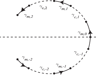
Figure 1. Left: Main and complementary arcs with $n=2$ (genus 4) for sech potential, where $f_{0}(z)$ has a jump across ${\mathbb{R}}$. Right: Deformation of main and complementary arcs into vertical branchcuts.

The scalar RHP (3.5) for $g(z;x,t)$ is completely defined if we know the genus $N$ of $\mathcal{R}$, the branchpoints $\alpha_{k}$ and the real constants $W_{j},\Omega_{j}$. From the point of view of solving RHP (3.5), the exact location of the main arcs $\gamma_{m,j}$ is not crucial, as, due to the analyticity of $f(z)$, they can be deformed without changing $g$.

The real constants in the RHP (3.5) are determined by the requirement that $g$ is analytic at $z=\infty$ and will be discussed in Section 5 below. What conditions determine the genus $N$ and the branchpoints? Without going into the details of $g$-function mechanism, we will state that the function

(3.13) $$h(z;x,t)=2g(z;x,t)-f(z;x,t)$$

must satisfy the following “sign distribution” conditions in ${\mathbb{C}}^{+}$:

(3.14) $$\Im h<0 \gamma_{m,j} j=0,1,\cdots,n$$ on both sides of each main arc , ,

(3.15) $$\Im h>0 \gamma_{c,j} j=1,\cdots,n$$ along each complementary arc , .

The corresponding inequalities in the lower half-plane, due to Schwarz symmetry, have the opposite signs.) Note that according to (3.5), (3.13), $h_{+}(z)+h_{-}(z)=2W_{j}$ on $\gamma_{m,j}$, so that all the main arcs lie on zero level curves of $\Im h(z)$. Conditions (3.14) can be violated in no more than a finite number of points. If this is the case, the corresponding value of $(x,t)=(x_{b},t_{b})$ is called a breaking point.

At any branchpoint, where a main and a complementary arcs meet (movable branchpoint), conditions (3.14), combined with (3.12), imply that

(3.17) $$\Im h(z;x,t)=O(z-a_{k})^{\frac{3}{2}}$$

Equations (3.17), are known in the RHP literature as the modulation equations (although they essentially are solutions of the (differential) Whitham equations), determine the location of all movable (with $x,t$) branchpoints. Fixed branchpoints (“hard edges”) are known to appear in some non-analytic cases (see, for example, [17], for the box initial data). If two or more branchpoints collide at some $\alpha$, we will have

(3.18) $$\Im h(z;x,t)=o(z-a_{k})^{\frac{3}{2}}$$

instead of (3.17). Now, the only remaining question is: how is the genus $N$ defined?

Usually, the genus $N$ is defined for some special values of $x,t$, say, for the initial data $t=0$. As we then continuously deform external parameters $x,t$, the branchpoints $\alpha_{j}$ move according to (3.17), pulling (deforming) main and complementary arcs of the contour $\gamma=\gamma(x,t)$ with them. The genus will be preserved under such deformation until a breaking point $(x_{b},t_{b})$ is reached. A regular breaking point is attained by changing the topology of the zero level of $\Im f(z;x,t)$, called pinching: the required inequalities (3.14) failed in one or several points on the main and/or complementary arcs. Such points are called double points. Another cause of breaking points is interaction of the Riemann-Hilbert contour of $g$ (the collection of the main and complementary arcs) with singularities of $f_{0}(z)$, or, in the case of piece-wise analytic $f_{0}(z)$, the interaction of the Riemann-Hilbert contour with various elements of $f_{0}(z)$.

The continuation principle ([29]) states that, in the case of a regular breaking point $(x_{b},t_{b})$, we can continue deformation of $x,t$ (with sign conditions satisfied) past $(x_{b},t_{b})$ with the appropriate change of the genus $N$.

The scalar RHP (3.5) and the modulation equations (3.17) is the starting point of our analysis. Various forms of Whitham equations from Section 2 and conservation equations can be derived from (3.5) and (3.17).

4. The genus 0 case

In the case of $n=0$ there are no real constants in the RHP (3.5). Then the modulation equations (3.17), defining the branchpoints of $\mathcal{R}(x,t)$, can be written as

(4.1) $$\oint_{\hat{\gamma}_{m}}{{f(\zeta)}\over{(\zeta-\alpha)R(\zeta)_{+}}}d\zeta=0~{},$$

and its complex conjugate, where $\alpha=\alpha_{0}$, $f$ is given by (3.9) and $\hat{\gamma}_{m}$ is a negatively (clockwise) oriented loop around the main arc (band) that intersects ${\mathbb{R}}$ only at some point $\mu$. Here $R(z)=\sqrt{(z-\alpha)(z-\bar{\alpha})}$.

Clearly, (4.1) and (3.9) yield

(4.2) $$2x+2(\Re\alpha+\alpha)t=-\frac{1}{2\pi i}\oint_{\hat{\gamma}_{m}}{{f_{0}(\zeta)}\over{(\zeta-\alpha)R(\zeta)_{+}}}d\zeta~{}$$

together with its complex conjugate. Comparison of (4.2) and the hodograph equation (2.11) yields

(4.3) $$V(\alpha,\bar{\alpha})=\frac{3}{2}(\alpha+\bar{\alpha}),~{}~{}~{}w(\alpha,\bar{\alpha})=-\frac{1}{4\pi i}\oint_{\hat{\gamma}_{m}}{{f_{0}(\zeta)}\over{(\zeta-\alpha)R(\zeta)_{+}}}d\zeta$$

and their complex conjugates, where the velocity coincides with (1.6). In the genus zero case there is only one Tsarev equation (2.12)

(4.4) $$\frac{\partial_{\bar{\alpha}}w}{w-\bar{w}}=\frac{\partial_{\bar{\alpha}}V}{V-\bar{V}}$$

and its complex conjugate, that can be shown true by immediate calculation. Thus, we proved that $\alpha,\bar{\alpha}$ satisfy the corresponding genus zero Whitham equations (1.6). In fact, (4.1) and its complex conjugate represent the hodograph solution to the Whitham equations (1.6).

According to (3.10) and (3.13), in the genus zero case

(4.5) $$h(z)=\frac{R(z)}{2\pi i}\oint_{\hat{\gamma}_{m}}{{f(\zeta)}\over{(\zeta-z)R(\zeta)_{+}}}d\zeta,$$

as there are no complementary arcs and the constants $W_{0}$ can be choosen as zero. Using

(4.6) $$\frac{\partial}{\partial\alpha}\frac{R(z)}{R(\zeta)}=\frac{1}{2}\frac{\zeta-z}{(z-\alpha)(\zeta-\alpha)}\frac{R(z)}{R(\zeta)}$$

and (4.5), we obtain

(4.7) $$\frac{\partial}{\partial\alpha}h(z)=\frac{R(z)}{2(z-\alpha)}\cdot\left.\frac{h(\zeta)}{R(\zeta)}\right|_{\zeta=a}$$

and its complex conjugate. Since, according to (4.1), the last fraction is equal to zero, we obtain

(4.8) $$\frac{\partial}{\partial\alpha}h(z)\equiv 0\Leftrightarrow{\rm modulation~{}equations}.$$

According to (4.8) and (3.9), we have

(4.9) $$h(z)=h(z;x,t,\alpha)=xh_{x}(z)+th_{t}(z)+h_{0},~{}~{}~{}{\rm where}~{}~{}~{}h_{0}=\frac{R(z)}{2\pi i}\oint_{\hat{\gamma}_{m}}{{f_{0}(\zeta)}\over{(\zeta-z)R(\zeta)_{+}}}d\zeta$$

and

(4.10) $$h_{x}(z)=2R(z),~{}~{}~{}~{}~{}~{}~{}~{}~{}~{}~{}~{}~{}~{}~{}h_{t}(z)=2(z+a)R(z)$$

were calculated in [30]. Here $a=\Re\alpha$ and $h_{x},h_{t}$ are partial derivatives in the corresponding variables, which, according to (4.8), coincide with “full” derivatives on the solutions of modulation equations $\alpha=\alpha(x,t)$. Obviously,

(4.11) $$\partial_{x}h_{t}\equiv\partial_{t}h_{x},$$

and one can check directly that this condition is equivalent to to the modulation equation (4.1). Moreover, $dh_{x}$, $dh_{t}$ are meromorphic differential of the second kind on $\mathcal{R}$ with the only poles at $\infty^{\pm}$ and, according to (2.2),

(4.12) $$dp=dh_{x},~{}~{}~{}dq=dh_{t}.$$

Thus, $p=h_{x}(z),q=h_{t}(z)$ are primitive functions for the meromorphic differentials $dp,dq$, and $h(z)$ is a potential for $p,q$. So, we come to the conclusion that the topology of zero level curves of the imaginary part of the potential for $p,q$ that is defined by a particular solution, determines the change of genus of Whitham equations.

5. Determinantal formula for $g$ when $f_{0}(z)$ is real analytic on an interval of ${\mathbb{R}}$

Consider the case when the (generally piece-wise) analytic function $f_{0}(z)$ does not have a jump on some interval $I\subset{\mathbb{R}}$. Let us assume for the moment that all the branchpoints $\alpha_{j}$ in the upper half-plane have distinct real parts Then, deforming the main and complementary arcs, as shown in Figure 1, Right, we can reduce the RHP (3.5) for $g(z)$ to the equivalent RHP with jumps along the vertical contours $\tilde{\gamma}_{j}$ with the branchpoints $\bar{\alpha}_{j},\alpha_{j}$, $j=0,\dots,N$:

(5.1) $$g_{+}+g_{-} =f+\tilde{\eta}_{j}~{}~{}\mbox{ on the vertical contour ${\tilde{\gamma}}_{j}$, $j=0,\cdots,N$}$$

(5.2) $$g(z) {\bar{\mathbb{C}}}\setminus\cup{\tilde{\gamma}}_{j}$$ is analytic in ,

where the real constants $\tilde{\eta}_{2j}$ are expressed as differences of constants $W,\Omega$ on the neighboring main and complementary arcs. For example, we have $\tilde{\eta}_{2j}=W_{j}-\Omega_{j+1}$, $\tilde{\eta}_{2j+1}=W_{j+1}-\Omega_{j+1}$ for the configuration, shown on Figure 1, Right. The $g$ functions, defined by the RHPs (3.5) and (5.1) coincide outside the region, encircled by the “old” main and complementary arcs and “new” vertical cuts (called bands), see Figure 1, Right. Inside this region, the “new” $g(z)$ coincides with: the “old” $g(z)$ up to appropriate real constant $\Omega_{j}$ on the positive (left) side of any two neighboring bands ${\tilde{\gamma}}$; the values of the “old” $g(z)$ from the second sheet of $\mathcal{R}$ up to appropriate real constant $W_{j}$ on the negative (right) side of any two neighboring bands ${\tilde{\gamma}}$ (note the opposite orientation of the neighboring bands). Thus, the modulation equations (3.17) remains valid for the “new” $g$, so that either RHP (3.5) or RHP (5.1) can be used to calculate the branchpoints $\alpha_{j}$, the Whitham equations, conservation equations, etc.

Introducing now $\tilde{g}=g-\frac{\tilde{\eta}_{0}}{2}$, we obtain the RHP

(5.4) $$\tilde{g}_{+}+\tilde{g}_{-} =f+\eta_{j}~{}~{}\mbox{ on the band ${\tilde{\gamma}}_{j}$, $j=0,\cdots,2n$}$$

(5.5) $$\tilde{g}(z) {\bar{\mathbb{C}}}\setminus\gamma$$ is analytic in ,

where $\eta_{2j}=\tilde{\eta}_{2j}-\tilde{\eta}_{0}$. In the configuration of Figure 1, Right, $\eta_{2j}=W_{j}-\Omega_{j+1}+\Omega_{1}$, $\eta_{2j+1}=W_{j+1}-\Omega_{j+1}+\Omega_{1}$. The constants $\boldsymbol{\eta}=(\eta_{1},\dots,\eta_{2n})$ are exactly the constants from the argument of the multi-phase nonlinear wave solution (given through the Riemann Theta function) of the model problem, see [30], Section 8. They are also introduced in (1.4) as fundamental phases. With a mild abuse of notation, we will use $g(z)$ instead of $\tilde{g}(z)$ below and use $\mathcal{R}$ to denote the hyperelliptic Riemann surface with branchcuts along ${\tilde{\gamma}}_{j}$. Here and henceforth we also assume that all the bands are oriented upwards. This orientation does not change any jump conditions (5.4).

Remark 5.1.

The vertical branchcuts ${\tilde{\gamma}}_{j}$ of $\mathcal{R}$ can be bent to avoid intersection of different ${\tilde{\gamma}}_{j}$, ${\tilde{\gamma}}_{k}$ when $\Re\alpha_{j}=\Re\alpha_{k}$. They can also be appropriately bent to intersect ${\mathbb{R}}$ within the interval $I\subset{\mathbb{R}}$, where $f_{0}(z)$ is real analytic.

.

Example 5.1.

In the case of the box potential, the piece-wise analytic function $f(z)$ is defined by

(5.7) $$f(z)=2tz^{2}+2z(x-L)+4kL\nu(z)~{}~{}~{}~{}{\rm on}~{}~{}~{}~{}{\tilde{\gamma}}_{2k}\cup{\tilde{\gamma}}_{2k+1},$$

see [18], where $\nu(z)=\sqrt{z^{2}+q^{2}}$. The number of the bands depends on the particular values of $(x,t)$.

In the case of genus not exceeding one, the $g$-function, defined by (5.4), coincides with the one from [17] up to a real constant. By Sokhotski-Plemelj formula, we have

(5.8) $$2g(z)={{R(z)}\over{2\pi i}}\left[\sum_{j=1}^{N}\oint_{\hat{\tilde{\gamma}}_{j}}{{\eta_{j}d\zeta}\over{(\zeta-z)R(\zeta)}}+\oint_{\cup\hat{\tilde{\gamma}}_{k}}{{f(\zeta)d\zeta}\over{(\zeta-z)R(\zeta)}}\right],$$

where $R(z)=\prod_{j=0}^{2n}\sqrt{(z-\alpha_{j})(z-\bar{\alpha}_{j})}$, $\hat{\tilde{\gamma}}_{j}$ denotes the negatively (clockwise) oriented loop around ${\tilde{\gamma}}_{j}$ and $f(z)$ is analytically continued from ${\tilde{\gamma}}_{j}$ to $\hat{\tilde{\gamma}}_{j}$. We assume the loops $\hat{\tilde{\gamma}}_{j}$ do not intersect each other. With a mild abuse of notation, we will keep using $\hat{\gamma}$ instead of $\hat{\tilde{\gamma}}$.

The $N$ real constants $\eta_{j}$, defined by the requirement that $g$ from (5.8) is analytic at infinity, satisfy the system of $N$ real linear equations

(5.9) $$\frac{1}{2\pi i}\oint_{\cup\hat{\gamma}_{j}}{\zeta^{k}{f(\zeta)}\over{R(\zeta)}}d\zeta+\frac{1}{2\pi i}\sum_{j=1}^{N}\oint_{\hat{\gamma}_{j}}{{\eta_{j}\zeta^{k}}\over{R(\zeta)}}d\zeta=0\ \ \ \ \ k=0,1,\cdots,N-1.$$

It is well known that the matrix of this system

(5.10) $$D=\left(\begin{matrix}\oint_{\hat{\gamma}_{1}}\frac{d\zeta}{R(\zeta)}&\cdots&\oint_{\hat{\gamma}_{1}}\frac{\zeta^{N-1}d\zeta}{R(\zeta)}\cr\cdots&\cdots&\cdots\cr\oint_{\hat{\gamma}_{N}}\frac{d\zeta}{R(\zeta)}&\cdots&\oint_{\hat{\gamma}_{N}}\frac{\zeta^{N-1}d\zeta}{R(\zeta)}\end{matrix}\right)$$

is invertible and its inverse matrix

(5.11) $$D^{-1}=\left(\varkappa_{m,j}\right)$$

consists of the coefficients of the normalized holomorphic differentials

(5.12) $$\omega_{j}(z)=\frac{\varkappa_{N,j}z^{N-1}+\dots+\varkappa_{1,j}}{R(z)}dz=\frac{p_{j}(z)dz}{R(z)},~{}~{}~{}~{}j=1,\dots,N$$

of the Riemann surface $\mathcal{R}$, defined by $\oint_{\hat{\gamma}_{m}}\omega_{k}=\delta_{mk}$, see (2.6).

Consider now the determinant

(5.13) $$K(z)=\frac{1}{2\pi i}\times\left|\begin{matrix}\oint_{\hat{\gamma}_{1}}\frac{d\zeta}{R(\zeta)}&\cdots&\oint_{\hat{\gamma}_{1}}\frac{\zeta^{N-1}d\zeta}{R(\zeta)}&\oint_{\hat{\gamma}_{1}}\frac{d\zeta}{(\zeta-z)R(\zeta)}\cr\cdots&\cdots&\cdots&\cdots\cr\oint_{\hat{\gamma}_{N}}\frac{d\zeta}{R(\zeta)}&\cdots&\oint_{\hat{\gamma}_{N}}\frac{\zeta^{N-1}d\zeta}{R(\zeta)}&\oint_{\hat{\gamma}_{N}}\frac{d\zeta}{(\zeta-z)R(\zeta)}\cr\oint_{\cup\hat{\gamma}_{j}}\frac{f(\zeta)d\zeta}{R(\zeta)}&\cdots&\oint_{\cup\hat{\gamma}_{j}}\frac{\zeta^{N-1}f(\zeta)d\zeta}{R(\zeta)}&\oint_{\cup\hat{\gamma}_{j}}\frac{f(\zeta)d\zeta}{(\zeta-z)R(\zeta)}\cr\end{matrix}\right|.$$

Multiplying the $j$-th row by $\eta_{j}$ and adding it to the last row for each $j=1,\dots,N$, we obtain, according to (5.8) and (5.9),

(5.14) $$2g(z)=\frac{R(z)}{|D|}K(z),~{}~{}~{}z\in S,~{}~{}~{}~{}h(z)-\eta_{j}=\frac{R(z)}{|D|}K(z),~{}~{}~{}~{}~{}~{}~{}~{}z~{}{\rm inside~{}the~{}loop~{}}\hat{\gamma}_{j},$$

where $S$ is a region in ${\mathbb{C}}$, consisting of the points that are outside any loop $\hat{\gamma}_{j}$, $j=0,\dots,N$.

Note that

(5.15) $$K(z)=\frac{h(z)-\eta_{j}}{R(z)}|D|$$

is analytic inside the loop $\hat{\gamma}_{j}$. Thus, according to (5.14), (5.13), the modulation equations for all movable branchpoints $\alpha_{k}$ become

(5.16) $$K(\alpha_{k})=0.$$

In the case of distinct branchpoints $\alpha_{j}$, considered in the paper, we have $K(z)$ having a simple zero at every movable branchpoint $\alpha_{k}$.

Equation (5.14) allows us to represent $g(z)$ near $z=\infty$ as

(5.17) $$g(z)=\sum_{j=0}^{\infty}g_{j}z^{-j}.$$

Indeed, expanding $R(z)=z^{N+1}\sum_{j=0}^{\infty}\hat{R}_{j}z^{-j}$, $\frac{K(z)}{2|D|}=z^{-1}\sum_{j=0}^{\infty}\hat{K}_{j}z^{-j}$, where

(5.18) $$\hat{K}_{m}=\frac{-1}{4\pi i|D|}\left|\begin{matrix}\oint_{\hat{\gamma}_{1}}\frac{d\zeta}{R(\zeta)}&\cdots&\oint_{\hat{\gamma}_{1}}\frac{\zeta^{N-1}d\zeta}{R(\zeta)}&\oint_{\hat{\gamma}_{1}}\frac{\zeta^{N+m}d\zeta}{R(\zeta)}\cr\cdots&\cdots&\cdots&\cdots\cr\oint_{\hat{\gamma}_{N}}\frac{d\zeta}{R(\zeta)}&\cdots&\oint_{\hat{\gamma}_{N}}\frac{\zeta^{N-1}d\zeta}{R(\zeta)}&\oint_{\hat{\gamma}_{N}}\frac{\zeta^{N+m}d\zeta}{R(\zeta)}\cr\oint_{\cup\hat{\gamma}_{j}}\frac{f(\zeta)d\zeta}{R(\zeta)}&\cdots&\oint_{\cup\hat{\gamma}_{j}}\frac{\zeta^{N-1}f(\zeta)d\zeta}{R(\zeta)}&\oint_{\cup\hat{\gamma}_{j}}\frac{\zeta^{N+m}f(\zeta)d\zeta}{R(\zeta)}\cr\end{matrix}\right|,$$

we obtain

(5.19) $$g(z)=z^{N}\sum_{j=0}^{\infty}(\sum_{m=0}^{j}\hat{R}_{m}\hat{K}_{j-m})z^{-j}.$$

Note that (5.18) was obtained by factoring $-z^{-1}$ from the last column of (5.13) and expanding $(1-\frac{\zeta}{z})^{-1}$. The condition that $g(z)=O(1)$ at infinity implies that the first $N$ coefficients in (5.19) are zeroes and we obtain (5.17), where $g_{j}=\sum_{m=0}^{j+N}\hat{R}_{m}\hat{K}_{j+N-m}$.

We can also use (5.13) to calculate the fundamental phases $\eta_{j}$. Indeed, taking the proper linear combinations of the first $N$ columns of $K$ in (5.13), we obtain

(5.20) $$K(z)=\frac{|D|}{2\pi i}\times\left|\begin{matrix}1&\cdots&0&\oint_{\hat{\gamma}_{1}}\frac{d\zeta}{(\zeta-z)R(\zeta)}\cr\cdots&\cdots&\cdots&\cdots\cr 0&\cdots&1&\oint_{\hat{\gamma}_{N}}\frac{d\zeta}{(\zeta-z)R(\zeta)}\cr\oint_{\cup\hat{\gamma}_{j}}\frac{f(\zeta)p_{1}(\zeta)d\zeta}{R(\zeta)}&\cdots&\oint_{\cup\hat{\gamma}_{j}}\frac{f(\zeta)p_{N}(\zeta)d\zeta}{R(\zeta)}&\oint_{\cup\hat{\gamma}_{j}}\frac{f(\zeta)d\zeta}{(\zeta-z)R(\zeta)}\cr\end{matrix}\right|,$$

which implies that

(5.21) $$\eta_{m}=-\oint_{\cup\hat{\gamma}_{j}}\frac{f(\zeta)p_{m}(\zeta)d\zeta}{R(\zeta)}=4\pi i\left[\beta_{m}t+\varkappa_{N,m}x\right]-\Upsilon_{m},$$

where (see (3.9))

(5.22) $$\beta_{m}=\varkappa_{N,m}\sum_{k=0}^{N}\Re\alpha_{k}+\varkappa_{N-1,m},~{}~{}~{}\Upsilon_{m}=-\oint_{\cup\hat{\gamma}_{j}}\frac{f_{0}(\zeta)p_{m}(\zeta)d\zeta}{R(\zeta)}.$$

Comparing (5.21) with (2.13) one can see that the phases $\Upsilon_{m}$ in (5.21) coincide with the “modulation phase shifts” introduced in Section 2 in order to provide consistency of the “torus” phases $\eta_{j}$ linearly depending on $x$ and $t$ with the kinematic definitions (2.10) of the local wavenumbers and frequencies. These phase shifts can be viewed as the key objects of the modulation analysis as they generate via (2.15) the generalized hodograph solution to the Whitham equations. The RHP approach offers a direct route to finding the phases $\Upsilon_{m}$ in terms of the scattering data $f_{0}$ of the initial potential, thus enabling one to circumvent the complicated matching regularization procedure. In particular, for the box potential we have

(5.23) $$\Upsilon_{m}=4L\left[i\pi\varkappa_{N,m}+\sum_{k=0}^{N}\oint_{\hat{\gamma}_{k}}\frac{[\frac{k}{2}]p_{m}(\zeta)\nu(\zeta)d\zeta}{R(\zeta)}\right].$$

To calculate (5.21)- (5.23) we used expansions

(5.24) $$\frac{1}{R(z)}= z^{-N-1}+{\Re\sum\alpha_{j}}z^{-N-2}+\dots~{}~{}~{}~{}$$

(5.25) $$(2tz^{2}+2xz)p_{j}(z)= 2t\varkappa_{N,j}z^{N+1}+\left[2x\varkappa_{N,j}+2t\varkappa_{N-1,j}\right]z^{N}+\dots.$$

In the next section we will show that expressions for $\Upsilon_{m}$ in (5.22) indeed generate, via (2.15), the required hodograph solution to the Whitham equations.

6. Whitham equations for movable branchpoints and their solutions

Theorem 6.1.

Let $\alpha$ denote an arbitrary branchpoint $\alpha_{j}$, $j=0,1,\dots,N$, or their complex conjugate, in the set of $2N+2$ distinct branchpoints. Then the following statements are equivalent: 1) $K(\alpha)=0$; 2) $\frac{\partial\vec{\eta}}{\partial\alpha}=0$; 3) $\frac{\partial g(z)}{\partial\alpha}\equiv 0$ for all $z\in{\mathbb{C}}$, where $\vec{\eta}=(\eta_{1},\dots,\eta_{N})$.

Proof.

Combining (5.8), (5.14), (5.13) with the identity

(6.1) $$\frac{\partial}{\partial\alpha}\left[\frac{R(z)}{(\zeta-z)R(\zeta)}\right]=-\frac{R(z)}{2(z-\alpha)(\zeta-\alpha)R(\zeta)},$$

we obtain

(6.2) $$2\frac{\partial g(z)}{\partial\alpha}=-\frac{R(z)K(\alpha)}{2(z-\alpha)|D|}+{{R(z)}\over{2\pi i}}\sum_{j=1}^{N}\frac{\partial\eta_{j}}{\partial\alpha}\oint_{\hat{\gamma}_{j}}{\frac{d\zeta}{(\zeta-z)R(\zeta)}},$$

where $z$ is outside all the loops $\hat{\gamma}_{j}$.

Equation (5.17) shows that

(6.3) $$\frac{\partial g(z)}{\partial\alpha}~{}~{}~{}{\rm is~{}analytic~{}at}~{}\infty.$$

Let $K(\alpha)=0$. Then (6.3) implies the system of linear equations

(6.4) $$\sum_{j=1}^{N}\frac{\partial\eta_{j}}{\partial\alpha}\oint_{\hat{\gamma}_{j}}{\frac{\zeta^{k}d\zeta}{R(\zeta)}}=0,~{}~{}~{}~{}k=0,1\dots,N-1$$

for $\frac{\partial\vec{\eta}}{\partial\alpha}$. Since the matrix $D$ of this system is invertible, see (5.11), and the right hand side is zero, the system (6.4) has only zero solution. Hence, we proved that 1) implies 2). Similarly, (6.3) combined with $\frac{\partial\vec{\eta}}{\partial\alpha}=0$ imply 3), that is, 2) implies 3).

Let us now assume 3), that is, $\frac{\partial g(z)}{\partial\alpha}\equiv 0$ for all $z\in{\mathbb{C}}$. Then, differentiating in $\alpha$ the jump conditions in (5.4) (away from the branchpoints), we obtain $\frac{\partial\vec{\eta}}{\partial\alpha}=0$. Now 1) follows from (6.2).

∎

Here and henceforth we assume that the modulation equations $K(\alpha_{j})=0$ and their complex conjugate hold for all movable branchpoints $\alpha_{j}$. As an immediate consequence of Theorem 6.1, we obtain the following corollary.

Corollary 6.1.

For any $j=1,\dots,N$ we now have (2.5), namely

(6.5) $$\frac{d}{dx}\eta_{j}=\frac{\partial}{\partial x}\eta_{j}=4\pi i\varkappa_{N,j}=k_{j},~{}~{}~{}~{}~{}~{}~{}\frac{d}{dt}\eta_{j}=\frac{\partial}{\partial t}\eta_{j}=4\pi i\left(\varkappa_{N,j}\sum_{k=0}^{N}\Re\alpha_{k}+\varkappa_{N-1,j}\right)=\omega_{j},$$

where $\frac{d}{dx}$, $\frac{d}{dt}$ denote full derivatives and $k_{j},\omega_{j}$ are given by (1.4).

The corollary follows directly from Theorem 6.1 and (5.21), (5.22). One can see that expressions (6.5) agree with the kinematic relations (2.10), which are introduced in the modulation theory as definitions of the local wavenumbers $k_{j}$ and the local frequencies $\omega_{j}$. Moreover, Theorem 6.1 implies the stationary phase conditions (2.16) that can be written in the form of hodograph equations (2.15). As earlier, the conservation of waves equations (2.8) follows from Clairaut’s theorem.

Corollary 6.2.

If all the branchpoints $\alpha_{j}$, $j=0,1,\dots,N$, and their complex conjugates are distinct, then

(6.6) $$\frac{d}{dx}g(z;x,t)=\frac{\partial}{\partial x}g(z;x,t),~{}~{}~{}~{}~{}\frac{d}{dt}g(z;x,t)=\frac{\partial}{\partial t}g(z;x,t),$$

where $\frac{d}{dx}$ of $g$ denotes the “full” derivative in $x$ that include $\sum_{j}\left(\frac{\partial}{\partial\alpha_{j}}\frac{\partial\alpha_{j}}{\partial x}+\frac{\partial}{\partial\bar{\alpha}_{j}}\frac{\partial\bar{\alpha}_{j}}{\partial x}\right)$. The same holds for $\frac{d}{dt}$ of $g$.

According to (5.14) and Corollary 6.2,

(6.7) $$2\frac{d}{dx}g(z;x,t)=\frac{R(z)}{|D|}\frac{\partial}{\partial x}K(z;x,t),~{}~{}~{}~{}~{}2\frac{d}{dt}g(z;x,t)=\frac{R(z)}{|D|}\frac{\partial}{\partial t}K(z;x,t),$$

where $z$ is outside all of the loops $\hat{\gamma}_{j}$ and

(6.8) $$\frac{d}{dx}h(z;x,t)-(\eta_{j})_{x}=\frac{R(z)}{|D|}\frac{\partial}{\partial x}K(z;x,t),~{}~{}~{}~{}~{}\frac{d}{dt}h(z;x,t)-(\eta_{j})_{t}=\frac{R(z)}{|D|}\frac{\partial}{\partial t}K(z;x,t),$$

where $z$ is inside any loop, see (3.13). Then, direct calculations show that

(6.9) $$\frac{\partial}{\partial x}K(z)=2\left|\begin{matrix}\oint_{\hat{\gamma}_{1}}\frac{d\zeta}{R(\zeta)}&\cdots&\oint_{\hat{\gamma}_{1}}\frac{\zeta^{N-2}d\zeta}{R(\zeta)}&\oint_{\hat{\gamma}_{1}}\frac{d\zeta}{(\zeta-z)R(\zeta)}\cr\cdots&\cdots&\cdots&\cdots\cr\oint_{\hat{\gamma}_{N}}\frac{d\zeta}{R(\zeta)}&\cdots&\oint_{\hat{\gamma}_{N}}\frac{\zeta^{N-2}d\zeta}{R(\zeta)}&\oint_{\hat{\gamma}_{N}}\frac{d\zeta}{(\zeta-z)R(\zeta)}\cr\end{matrix}\right|+\frac{2z|D|}{R(z)}\chi_{S}(z)$$

and

(6.10) $$\begin{split}\frac{\partial}{\partial t}K(z)=2\left|\begin{matrix}\oint_{\hat{\gamma}_{1}}\frac{d\zeta}{R(\zeta)}&\cdots&\oint_{\hat{\gamma}_{1}}\frac{\zeta^{N-3}d\zeta}{R(\zeta)}&\oint_{\hat{\gamma}_{1}}\frac{d\zeta}{(\zeta-z)R(\zeta)}&\oint_{\hat{\gamma}_{1}}\frac{\zeta^{N-1}d\zeta}{R(\zeta)}\cr\cdots&\cdots&\cdots&\cdots&\cdots\cr\oint_{\hat{\gamma}_{N}}\frac{d\zeta}{R(\zeta)}&\cdots&\oint_{\hat{\gamma}_{N}}\frac{\zeta^{N-3}d\zeta}{R(\zeta)}&\oint_{\hat{\gamma}_{N}}\frac{d\zeta}{(\zeta-z)R(\zeta)}&\oint_{\hat{\gamma}_{N}}\frac{\zeta^{N-1}d\zeta}{R(\zeta)}\cr\end{matrix}\right|\\ +2\sum_{j=0}^{2N}\Re\alpha_{j}\frac{\partial}{\partial x}K(z)+\frac{2z^{2}|D|}{R(z)}\chi_{S}(z)~{}.\end{split}$$

where $\chi_{S}(z)$ denotes the characteristic function of the set $S$, which contains all the points of $\bar{\mathbb{C}}$ outside the loops. Since we will evaluate $\frac{\partial}{\partial x}K(z)$, $\frac{\partial}{\partial t}K(z)$ mostly at the branchpoints, we should disregard the last terms in (6.9), (6.10) in the formulae below.

Lemma 6.1.

Functions $\frac{\partial}{\partial x}h(z;x,t)$, $\frac{\partial}{\partial t}h(z;x,t)$ are meromorphic on $\mathcal{R}$ with the only poles at $\infty^{\pm}$ and attaining the values

(6.11) $$h_{x}(\alpha_{j})=h_{x}(\bar{\alpha}_{j})=(\eta_{j})_{x},~{}~{}~{}~{}~{}h_{t}(\alpha_{j})=h_{t}(\bar{\alpha}_{j})=(\eta_{j})_{t},~{}~{}~{}~{}j=0,1,\dots,N,$$

where $\eta_{0}=0$.

Proof.

According to (6.7) and (6.9), (6.10), functions $\frac{\partial}{\partial x}g(z;x,t)$, $\frac{\partial}{\partial t}g(z;x,t)$ are analytic on $S$, where analyticity at $z=\infty$ can be shown by differentiating (5.17). Let us collapse the loops $\hat{\gamma}_{j}$ onto the bands ${\tilde{\gamma}}_{j}$, $j=0,\dots,N$, that are the branchcuts of $\mathcal{R}$. Then $\frac{\partial}{\partial x}g(z;x,t)$, $\frac{\partial}{\partial t}g(z;x,t)$ will be analytic on $S=\bar{\mathbb{C}}\setminus\cup_{0}^{\infty}{\tilde{\gamma}}_{j}$.

Let us fix some $z\in{\tilde{\gamma}}_{j}$ and denote by $g_{\pm}(z),h_{\pm}(z)$ the limiting values of $g,h$ as we collapse $\hat{\gamma}_{j}$ onto ${\tilde{\gamma}}_{j}$. Then, according to (6.7)-(6.10),

(6.12) $$\begin{split}&2(g_{x})_{+}-[(h_{x})_{+}-(\eta_{j})_{x}]=2z+(\eta_{j})_{x},~{}~{}~{}~{}~{}~{}~{}~{}{\rm on}~{}~{}\hat{\gamma}_{j},~{}~{}~{}{\rm to~{}the~{}left~{}of}~{}~{}{\tilde{\gamma}}_{j}\\ &2(g_{x})_{-}-[(h_{x})_{-}-(\eta_{j})_{x}]=2z+(\eta_{j})_{x},~{}~{}~{}~{}~{}~{}~{}~{}{\rm on}~{}~{}\hat{\gamma}_{j}~{}~{}~{}{\rm to~{}the~{}right~{}of}~{}~{}{\tilde{\gamma}}_{j},\\ &(h_{x})_{+}-(\eta_{j})_{x}+(h_{x})_{-}-(\eta_{j})_{x}=0,~{}~{}~{}~{}~{}~{}~{}{\rm on}~{}~{}{\tilde{\gamma}}_{j},~{}~{}~{}~{}\end{split}$$

so, adding these jumps, we obtain

(6.13) $$(g_{x})_{+}+(g_{x})_{-}=2z+(\eta_{j})_{x}~{}~{}\mbox{ on the band ${\tilde{\gamma}}_{j}$, $j=0,\cdots,N$}.$$

Similarly,

(6.14) $$(g_{t})_{+}+(g_{t})_{-}=2z^{2}+(\eta_{j})_{t}~{}~{}\mbox{ on the band ${\tilde{\gamma}}_{j}$, $j=0,\cdots,N$}.$$

Note also that, according to (6.7)-(6.10), the limiting values $(g_{x})_{\pm},(g_{t})_{\pm}$ on the branchcuts ${\tilde{\gamma}}_{j}$ are continuous and bounded functions. So, $g_{x},g_{t}$ satisfy the RHPs similar to (5.4), and, correspondingly, can be written as

(6.15) $$\frac{\partial g(z)}{\partial x}=z+{{R(z)}\over{4\pi i}}\sum_{j=1}^{N}\oint_{\hat{\gamma}_{j}}{\frac{(\eta_{j})_{x}d\zeta}{(\zeta-z)R_{+}(\zeta)}},~{}~{}~{}~{}~{}~{}\frac{\partial g(z)}{\partial t}=z^{2}+{{R(z)}\over{4\pi i}}\sum_{j=1}^{N}\oint_{\hat{\gamma}_{j}}{\frac{(\eta_{j})_{t}d\zeta}{(\zeta-z)R_{+}(\zeta)}}.$$

Thus,

(6.16) $$\frac{\partial h(z)}{\partial x}=\frac{\partial g(z)}{\partial x}-2z,~{}~{}~{}\frac{\partial h(z)}{\partial t}=\frac{\partial g(z)}{\partial t}-2z^{2}$$

are meromorphic on $\mathcal{R}$ with the only poles at $\infty^{\pm}$. Equations (6.11) follow from (6.8). ∎

This lemma could also be proven using the fact that the RHP (5.4) for $g(z)$ commutes with $\frac{d}{dx}$, $\frac{d}{dt}$, because the boundary values $g_{\pm}$, as well as $(g_{x})_{\pm},(g_{t})_{\pm}$ belong to $L^{2}_{loc}$ along the jump contours $\cup_{j=0}^{N}{\tilde{\gamma}}_{j}$.

In the particular case of $N=2$, we have

(6.17) $$\frac{\partial}{\partial x}K(z)=-2\left|\begin{matrix}\oint_{\hat{\gamma}_{1}}\frac{d\zeta}{(\zeta-z)R(\zeta)}&\oint_{\hat{\gamma}_{1}}\frac{d\zeta}{R(\zeta)}\cr\oint_{\hat{\gamma}_{2}}\frac{d\zeta}{(\zeta-z)R(\zeta)}&\oint_{\hat{\gamma}_{2}}\frac{d\zeta}{R(\zeta)}\end{matrix}\right|$$

and

(6.18) $$\frac{\partial}{\partial t}K(z)=2\left|\begin{matrix}\oint_{\hat{\gamma}_{1}}\frac{d\zeta}{(\zeta-z)R(\zeta)}&\oint_{\hat{\gamma}_{1}}\frac{\zeta d\zeta}{R(\zeta)}\cr\oint_{\hat{\gamma}_{2}}\frac{d\zeta}{(\zeta-z)R(\zeta)}&\oint_{\hat{\gamma}_{2}}\frac{\zeta d\zeta}{R(\zeta)}\end{matrix}\right|+2\sum_{j=0}^{2}\Re\alpha_{j}\frac{\partial}{\partial x}K(z)$$

Lemma 6.2.

Let $\alpha$ denote any movable $\alpha_{j}$, $j=0,1,\dots,N$, or its complex conjugate, and the modulation equations (5.16) hold. Then

(6.19) $$\frac{\partial K(z)}{\partial\alpha}=\left[\frac{\partial\ln|D|}{\partial\alpha}+\frac{1}{2(z-\alpha)}\right]K(z).$$

In particular, if $\beta$ denote another movable branchpoint, then

(6.20) $$\frac{\partial}{\partial\alpha}K(\beta)=0~{}~{}~{}~{}{\rm if}~{}~{}~{}~{}\alpha\neq\beta~{}~{}~{}{\rm and}~{}~{}\frac{\partial}{\partial\alpha}K(\alpha)=\frac{1}{2}K^{\prime}(z)|_{z=\alpha}.$$

Proof.

Formula (6.19) a direct consequence of Theorem 6.1 and (5.14), whereas (6.20) follows from (5.13), (5.16) and analyticity of $K(z)$ at $z=\alpha_{j}$. ∎

As a consequence of Lemma 6.2 and the modulation equations (5.16), we obtain

(6.21) $$\frac{\partial K(\alpha_{j})}{\partial\alpha_{j}}(\alpha_{j})_{x}=-\frac{\partial}{\partial x}K(\alpha_{j}),~{}~{}~{}~{}~{}~{}~{}~{}~{}~{}~{}\frac{\partial K(\alpha_{j})}{\partial\alpha_{j}}(\alpha_{j})_{t}=-\frac{\partial}{\partial t}K(\alpha_{j})~{},~{}~{}~{}~{}~{}$$

for any movable branchpoint $\alpha_{j}$ and its complex conjugate. Thus, we obtain the corresponding Whitham partial differential equations

(6.22) $$(\alpha_{j})_{t}=V_{j}({\boldsymbol{\alpha}},\boldsymbol{\bar{\alpha}})(\alpha_{j})_{x},~{}~{}{\rm where}~{}~{}V_{j}({\boldsymbol{\alpha}},\boldsymbol{\bar{\alpha}})=\frac{\frac{\partial}{\partial t}K(\alpha_{j})}{\frac{\partial}{\partial x}K(\alpha_{j})}~{}~{}$$

as it was stated in (1.5), Section 1.

We also obtain the ordinary differential equations

(6.23) $$\partial_{t}(\alpha_{j})=-\frac{2\partial_{t}K(\alpha_{j})}{K^{\prime}(\alpha_{j})},~{}~{}~{}~{}~{}~{}~{}\partial_{x}(\alpha_{j})=-\frac{2\partial_{x}K(\alpha_{j})}{K^{\prime}(\alpha_{j})},$$

for (time) trajectories and (space) isochrones of any movable branchpoint. Note that, according to Lemma 6.2, $(\alpha_{j})_{x},(\alpha_{j})_{t}$ are bounded provided that all the branchpoints are distinct.

Using the fact that $f(z)$ in the last row of the determinant $K$ in (5.13) is linear in $x,t$, we can rewrite the modulation equations (5.16) for movable singularities $\alpha_{j}$ and their complex conjugates as

(6.24) $${K_{x}(\alpha_{j})}x+{K_{t}(\alpha_{j})}t+{K_{0}(\alpha_{j})}=0,~{}~{}~{}~{}$$

where $K_{0}(z)$ is obtained from $K(z)$ by replacing $f(\zeta)$ with $f_{0}(\zeta)$. Equation (6.24) is another form of the hodograph equations (see (2.11))

(6.25) $$x+V_{j}t=w_{j},~{}~{}~{}~{}~{}~{}{\rm where}~{}~{}~{}V_{j}=\frac{K_{t}(\alpha_{j})}{K_{x}(\alpha_{j})}~{}~{}~{}{\rm and}~{}~{}w_{j}=-\frac{K_{0}(\alpha_{j})}{K_{x}(\alpha_{j})}.$$

Using (5.20), we obtain

(6.26) $$K_{x}(z) =-2|D|\sum_{j=1}^{N}\varkappa_{N,j}\oint_{\hat{\gamma}_{j}}\frac{d\zeta}{(\zeta-z)R(\zeta)}d\zeta,$$

(6.27) $$K_{t}(z) =-2|D|\sum_{j=1}^{N}\left(\varkappa_{N,j}\Re\sum_{k=1}^{N}\alpha_{k}+\varkappa_{N-1,j}\right)\oint_{\hat{\gamma}_{j}}\frac{d\zeta}{(\zeta-z)R(\zeta)}d\zeta.$$

Then, according to (6.25), we obtain the following new expressions for the characteristic velocities

(6.28) $$V_{j}=\frac{(\alpha_{j})_{t}}{(\alpha_{j})_{x}}=\frac{K_{t}(\alpha_{j})}{K_{x}(\alpha_{j})}=\Re\sum_{k=1}^{N}\alpha_{k}+\dfrac{\sum_{k=1}^{N}\varkappa_{N-1,k}\oint_{\hat{\gamma}_{k}}\frac{d\zeta}{(\zeta-\alpha_{j})R(\zeta)}d\zeta}{\sum_{k=1}^{N}\varkappa_{N,k}\oint_{\hat{\gamma}_{k}}\frac{d\zeta}{(\zeta-\alpha_{j})R(\zeta)}d\zeta}$$

in terms of the meromorphic differentials on $\mathcal{R}$. Tsarev equations (2.12) for $w_{j}$ follow immediately from (6.25).

Lemma 6.3.

If

(6.29) $$p=-\frac{1}{2}h_{x}=z-g_{x}(z),~{}~{}~{}q=-\frac{1}{2}h_{t}=z^{2}-g_{t}(z)$$

then differentials $dp,dq$ are fundamental meromorphic differentials, uniqely determined by the conditions a)-c) at the beginning of Section 2, see (2.2), (2.3).

Proof.

According to Lemma 6.1, $p,q$ are meromorphic on the hyperelliptic surface $\mathcal{R}$, with the only poles at $\infty^{\pm}$. Then

(6.30) $$dp=-\frac{1}{2}h_{xz}dz=(1-g_{xz}(z))dz,~{}~{}~{}dq=-\frac{1}{2}h_{tz}dz=(2z-g_{tz}(z))dz$$

are meromorphic differentials of the second kind with the only poles at $\infty^{\pm}$ satisfying (2.2).

To prove the normalization (2.3) of $dp,dq$, we notice that ${\tilde{\gamma}}_{j}$, $j=1,\dots,N$ are the ${\mathbf{A}}$-cycles of $\mathcal{R}$ and

(6.31) $$\oint_{{\tilde{\gamma}}_{j}}dp=-\int_{\bar{\alpha}_{j}}^{\alpha_{j}}h_{xz}dz=h_{x}(\bar{\alpha}_{j})-h_{x}(\alpha_{j})=0,$$

the latter follows from (6.11). Similar argument based on (6.8), (6.10) works for $dq$. ∎

Corollary 6.3.

The generating conservation equation $\partial_{t}dp=\partial_{x}dq$, see (2.1), is obviously true, as now it reduces to $h_{xzt}=h_{tzx}$ (or $g_{xzt}=g_{tzx}$).

Since the cycle $\mathbf{B_{j}}$ is a path, connecting $\alpha_{j}$ with $\alpha_{0}$ and returning back on the second sheet of $\mathcal{R}$, we obtain (2.4) by

(6.32) $$\begin{split}\oint_{\mathbf{B_{j}}}dp=-\int_{\alpha_{j}}^{\alpha_{0}}h_{xz}dz=h_{x}(\alpha_{j})-h_{x}(\alpha_{0})=(\eta_{j})_{x}=k_{j},\\ \oint_{\mathbf{B_{j}}}dq=-\int_{\alpha_{j}}^{\alpha_{0}}h_{tz}dz=h_{t}(\alpha_{j})-h_{t}(\alpha_{0})=(\eta_{j})_{t}=\omega_{j},\end{split}$$

where we used (6.11).

Finally, to prove (2.7), we notice that at any movable branchpoint $\alpha_{j}$ (and its c.c.)

(6.33) $$h_{xz}(z)=\frac{(R^{2}(z))^{\prime}}{2|D|R(z)}K_{x}(\alpha_{j})+O(z-\alpha_{j})^{\frac{1}{2}},~{}~{}~{}~{}~{}h_{tz}(z)=\frac{(R^{2}(z))^{\prime}}{2|D|R(z)}K_{t}(\alpha_{j})+O(z-\alpha_{j})^{\frac{1}{2}},$$

as $z\rightarrow\alpha_{j}$. Then, according to (6.30), (6.33) and (6.22),

(6.34) $$\left.\frac{dq}{dp}\right|_{\alpha_{j}}=\left.\frac{h_{tz}}{h_{xz}}\right|_{\alpha_{j}}=\frac{K_{t}(\alpha_{j})}{K_{x}(\alpha_{j})}=V_{j}.$$

So, we proved (2.7).

7. Determinantal formula for $g$ when $f_{0}(z)$ has a jump on ${\mathbb{R}}$

In the case when n $f_{0}(z)$ has a jump on ${\mathbb{R}}$ we have to work with the RHP (3.5) for the $g$-function. Similarly to (5.9), the real constants $W_{j},\Omega_{j}\in{\mathbb{R}}$, $j=1,2,\cdots,n$ in (3.10) are defined by

(7.1) $$\sum_{j=1}^{n}\frac{W_{j}}{2\pi i}\oint_{\hat{\gamma}_{m,j}}\frac{\zeta^{k}d\zeta}{R(\zeta)}+\sum_{j=1}^{n}\frac{\Omega_{j}}{2\pi i}\oint_{\hat{\gamma}_{c,j}}{{\zeta^{k}d\zeta}{R(\zeta)}}=\frac{1}{2\pi i}\sum_{j=1}^{n}\oint_{\hat{\gamma}_{m,j}}\frac{\zeta^{k}f(\zeta)d\zeta}{R(\zeta)}\ \ \ \ \ k=0,1,\cdots,2n-1.$$

This is a system of $N=2n$ real linear equations for $2n$ real unknowns $W_{j},\Omega_{j}$ that can be written as

(7.2) $$(\vec{W},\vec{\Omega})D=\vec{f},$$

where $\vec{W},\vec{\Omega}\in{\mathbb{R}}^{n}$ are row vectors with components $W_{j},\Omega_{j}$ respectively, $\vec{f}\in{\mathbb{R}}^{2n}$ denotes the row vector of the right hand sides of (7.1) multiplied by $2\pi i$, and

(7.3) $$D=\left(\begin{matrix}\oint_{\hat{\gamma}_{m,1}}\frac{d\zeta}{R(\zeta)}&\cdots&\oint_{\hat{\gamma}_{m,1}}\frac{\zeta^{2n-1}d\zeta}{R(\zeta)}\cr\cdots&\cdots&\cdots\cr\oint_{\hat{\gamma}_{m,n}}\frac{d\zeta}{R(\zeta)}&\cdots&\oint_{\hat{\gamma}_{m,n}}\frac{\zeta^{2n-1}d\zeta}{R(\zeta)}\cr\oint_{\hat{\gamma}_{c,1}}\frac{d\zeta}{R(\zeta)}&\cdots&\ \oint_{\hat{\gamma}_{c,1}}\frac{\zeta^{2n-1}d\zeta}{R(\zeta)}\cr\cdots&\cdots&\cdots\cr\oint_{\hat{\gamma}_{c,n}}\frac{d\zeta}{R(\zeta)}&\cdots&\oint_{\hat{\gamma}_{c,n}}\frac{\zeta^{N-1}d\zeta}{R(\zeta)}\cr\end{matrix}\right)~{}$$

It was shown in [28] that if all the branchpoints are distinct then $|D|\neq 0$.

Let us assume, for simplicity, that the function $f_{0}(z)$ is analytic in some region containing all the $\gamma^{+}_{m,j}$ Introducing the determinant $K(z)=K(z;x,t)$ by

(7.4) $$K(z)=\frac{1}{2\pi i}\times\left|\begin{matrix}\oint_{\hat{\gamma}_{m,1}}\frac{d\zeta}{R(\zeta)}&\cdots&\oint_{\hat{\gamma}_{m,1}}\frac{\zeta^{2n-1}d\zeta}{R(\zeta)}&\oint_{\hat{\gamma}_{m,1}}\frac{d\zeta}{(\zeta-z)R(\zeta)}\cr\cdots&\cdots&\cdots&\cdots\cr\oint_{\hat{\gamma}_{m,n}}\frac{d\zeta}{R(\zeta)}&\cdots&\oint_{\hat{\gamma}_{m,n}}\frac{\zeta^{2n-1}d\zeta}{R(\zeta)}&\oint_{\hat{\gamma}_{m,n}}\frac{d\zeta}{(\zeta-z)R(\zeta)}\cr\oint_{\hat{\gamma}_{c,1}}\frac{d\zeta}{R(\zeta)}&\cdots&\oint_{\hat{\gamma}_{c,1}}\frac{\zeta^{2n-1}d\zeta}{R(\zeta)}&\oint_{\hat{\gamma}_{c,1}}\frac{d\zeta}{(\zeta-z)R(\zeta)}\cr\cdots&\cdots&\cdots&\cdots\cr\oint_{\hat{\gamma}_{c,n}}\frac{d\zeta}{R(\zeta)}&\cdots&\oint_{\hat{\gamma}_{c,n}}\frac{\zeta^{2n-1}d\zeta}{R(\zeta)}&\oint_{\hat{\gamma}_{c,n}}\frac{d\zeta}{(\zeta-z)R(\zeta)}\cr\oint_{\hat{\gamma}}\frac{f(\zeta)d\zeta}{R(\zeta)}&\cdots&\oint_{\hat{\gamma}}\frac{\zeta^{2n-1}f(\zeta)d\zeta}{R(\zeta)}&\oint_{\hat{\gamma}}\frac{f(\zeta)d\zeta}{(\zeta-z)R(\zeta)}\cr\end{matrix}\right|,$$

we observe that, according to (7.2), (3.10),

(7.5) $$2g(z)=\frac{R(z)}{|D|}K(z),~{}~{}~{}~{}z~{}{\rm outside}~{}\hat{\gamma},~{}~{}~{}~{}h(z)-\eta_{j}=\frac{R(z)}{|D|}K(z),~{}~{}~{}~{}~{}~{}~{}~{}z~{}{\rm inside~{}}\hat{\gamma}{\rm~{}but~{}outside}~{}\hat{\gamma}_{j}$$

for all $j=1,\dots,N$. here the negatively oriented contour $\hat{\gamma}$ is going around all the all main arcs (it is pinched to $\gamma_{m,0}$ at $\mu$, where $\{\mu\}=\gamma_{m,0}\cap{\mathbb{R}}$).

Combining this considerations with (4.1), we obtain a new form of modulation equations

(7.6) $$K(\alpha_{j})=0,~{}~{}~{}~{}~{}~{}~{}j=0,1,\cdots,4n+1~{}.$$

We can now state Theorem (6.1) for the $g$-function, defined by the RHP (3.5).

Theorem 7.1.

Let $\alpha$ denote an arbitrary branchpoint $\alpha_{j}$, $j=0,1,\dots,4n+1$, in the set of $4n+2$ distinct branchpoints. Then the following statements are equivalent: 1) $K(\alpha)=0$; 2) $\frac{\partial(\vec{W},\vec{\Omega})^{t}}{\partial\alpha}=0$; 3) $\frac{\partial g(z)}{\partial\alpha}\equiv 0$ for all $z\in{\mathbb{C}}$.

The proof of the theorem is almost identical to that of Theorem (6.1). As an immediate consequence of Theorem (7.1), we obtain

(7.7) $$\frac{d}{dx}h(z;x,t)=\frac{R(z)}{|D|}\frac{\partial}{\partial x}K(z;x,t),~{}~{}~{}~{}~{}\frac{d}{dt}h(z;x,t)=\frac{R(z)}{|D|}\frac{\partial}{\partial t}K(z;x,t),$$

where $z$ is inside $\hat{\gamma}$ but outside all the loops $\hat{\gamma}_{m,j},\hat{\gamma}_{c,j}$. Without any lost of generality, we can take limit when contour $\hat{\gamma}$ in (7.4) becomes infinitely large. Then, direct calculations show that

(7.8) $$\frac{\partial}{\partial x}K(z)=\left|\begin{matrix}\oint_{\hat{\gamma}_{m,1}}\frac{d\zeta}{R(\zeta)}&\cdots&\oint_{\hat{\gamma}_{m,1}}\frac{\zeta^{2n-2}d\zeta}{R(\zeta)}&\oint_{\hat{\gamma}_{m,1}}\frac{d\zeta}{(\zeta-z)R(\zeta)}\cr\cdots&\cdots&\cdots&\cdots\cr\oint_{\hat{\gamma}_{m,n}}\frac{d\zeta}{R(\zeta)}&\cdots&\oint_{\hat{\gamma}_{m,n}}\frac{\zeta^{2n-2}d\zeta}{R(\zeta)}&\oint_{\hat{\gamma}_{m,n}}\frac{d\zeta}{(\zeta-z)R(\zeta)}\cr\oint_{\hat{\gamma}_{c,1}}\frac{d\zeta}{R(\zeta)}&\cdots&\oint_{\hat{\gamma}_{c,1}}\frac{\zeta^{2n-2}d\zeta}{R(\zeta)}&\oint_{\hat{\gamma}_{c,1}}\frac{d\zeta}{(\zeta-z)R(\zeta)}\cr\cdots&\cdots&\cdots&\cdots\cr\oint_{\hat{\gamma}_{c,n}}\frac{d\zeta}{R(\zeta)}&\cdots&\oint_{\hat{\gamma}_{c,n}}\frac{\zeta^{2n-2}d\zeta}{R(\zeta)}&\oint_{\hat{\gamma}_{c,n}}\frac{d\zeta}{(\zeta-z)R(\zeta)}\cr\end{matrix}\right|$$

and

(7.9) $$\frac{\partial}{\partial t}K(z)=-2\left|\begin{matrix}\oint_{\hat{\gamma}_{m,1}}\frac{d\zeta}{R(\zeta)}&\cdots&\oint_{\hat{\gamma}_{m,1}}\frac{\zeta^{2n-3}d\zeta}{R(\zeta)}&\oint_{\hat{\gamma}_{m,1}}\frac{d\zeta}{(\zeta-z)R(\zeta)}&\oint_{\hat{\gamma}_{m,1}}\frac{\zeta^{2n-1}d\zeta}{R(\zeta)}\cr\cdots&\cdots&\cdots&\cdots&\cdots\cr\oint_{\hat{\gamma}_{m,n}}\frac{d\zeta}{R(\zeta)}&\cdots&\oint_{\hat{\gamma}_{m,n}}\frac{\zeta^{2n-3}d\zeta}{R(\zeta)}&\oint_{\hat{\gamma}_{m,n}}\frac{d\zeta}{(\zeta-z)R(\zeta)}&\oint_{\hat{\gamma}_{m,n}}\frac{\zeta^{2n-1}d\zeta}{R(\zeta)}\cr\oint_{\hat{\gamma}_{c,1}}\frac{d\zeta}{R(\zeta)}&\cdots&\oint_{\hat{\gamma}_{c,1}}\frac{\zeta^{2n-3}d\zeta}{R(\zeta)}&\oint_{\hat{\gamma}_{c,1}}\frac{d\zeta}{(\zeta-z)R(\zeta)}&\oint_{\hat{\gamma}_{c,1}}\frac{\zeta^{2n-1}d\zeta}{R(\zeta)}\cr\cdots&\cdots&\cdots&\cdots&\cdots\cr\oint_{\hat{\gamma}_{c,n}}\frac{d\zeta}{R(\zeta)}&\cdots&\oint_{\hat{\gamma}_{c,n}}\frac{\zeta^{2n-3}d\zeta}{R(\zeta)}&\oint_{\hat{\gamma}_{c,n}}\frac{d\zeta}{(\zeta-z)R(\zeta)}&\oint_{\hat{\gamma}_{c,n}}\frac{\zeta^{2n-1}d\zeta}{R(\zeta)}\cr\end{matrix}\right|+\sum_{j=0}^{4n+1}\alpha_{j}\frac{\partial}{\partial x}K(z)~{}.$$

Collapsing the loops $\hat{\gamma}_{m,j},\hat{\gamma}_{c,j}$ back to the main and complementary arcs $\gamma_{m,j},\gamma_{c,j}$ respectively, we find that $h_{x}(z)$ satisfy the RHP with jumps and asymptotics

(7.10) $$(h_{x})_{+}+(h_{x})_{-} =2W_{j}~{}~{}\mbox{ on the main arc $\gamma_{m,j}$, $j=0,\cdots,n$}$$

(7.11) $$(h_{x})_{+}-(h_{x})_{-} =2\Omega_{j}~{}~{}\mbox{ on the complementary arc $\gamma_{c,j}$, $j=0,1,\cdots,n$ }$$

(7.12) $$h_{x}=-2z+O(1) ~{}~{}\mbox{as}z\rightarrow\infty$$

(7.13) .

The similar RHP is satisfied by $h_{t}(z)$. It also follows from (7.7), (7.8), (7.9) that $h_{x},h_{t}$ are bounded at the branchpoints.

We can now deform contours $\gamma_{m,j},\gamma_{c,j}$ in the same way as we did in the beginning of Section 5, to obtain jumps of $h_{x},h_{t}$ on $N+1$ vertical bands ${\tilde{\gamma}}_{j},$ $j=0,\dots,N$, where $N=2n$. These jumps $2(\eta_{k})_{x},2(\eta_{k})_{t}$ are given by $(\eta_{2j})_{x}=(W_{j})_{x}-(\Omega_{j+1})_{x}+(\Omega_{1})_{x}$, $(\eta_{2j+1})_{x}=(W_{j+1})_{x}-(\Omega_{j+1})_{x}+(\Omega_{1})_{x}$ and similar expressions for $2(\eta_{k})_{t}$. Solutions $h_{x}(z),h_{t}(z)$ to these deformed RHPs are meromorphic functions on the corresponding hyperelliptic surface $\mathcal{R}$ and their differentials, $dp=-\frac{1}{2}h_{xz}dz$, $dq=-\frac{1}{2}h_{tz}dz$, satisfy conditions a)-c) from Section 2. Thus, the results of Section 5 are also valid in our case.

8. Phase transitions and characteristic velocities along breaking curves

As we move in the $(x,t)$ (physical) plane along some (smooth) curve $\varpi$, the (movable) branchpoints $\alpha_{j}=\alpha_{j}(x,t)$ move in the $z$ (spectral) plane according to the modulation (Whitham) equations. As they move, the function $h(z;x,t)=h^{N}(z;x,t)$, where $N$ denotes the genus, changes according to (5.14) (or (7.5)) and, at some point $(x_{b},t_{b})\in\varpi$, called a breaking point, one (or more) of the inequalities (3.14) can fail at a some point $z_{0}$ (or at several points). Note that if $z_{0}\not\in{\mathbb{R}}$, then (3.14) should also fail at $\bar{z}_{0}$ due to Schwarz symmetry of $h^{N}$. Assuming that $h^{N}(z)$ is analytic at $z_{0}$, we readily obtain that

(8.1) $$h^{N}_{z}(z_{0})=0~{}~{}\qquad~{}~{}{\rm and}~{}~{}\qquad~{}\Im h^{N}(z_{0})=0$$

form a system of 3 real equations for 4 real variables ($x,t,z_{0}$) that determines the breaking curve. The point $z_{0}$ is called a double point. If $z_{0}\in\gamma_{m,j}$, then two new complementary arcs open at $z_{0}$ and at $\bar{z}_{0}$ as we cross the breaking curve and the genus of $\mathcal{R}=\mathcal{R}(x,t)$ increases by two. (Generically, it will increase only by one if $z_{0}\in{\mathbb{R}}$.) Similarly, if $z_{0}\in\gamma_{c,j}$, two new main arcs open at $z_{0}$ and at $\bar{z}_{0}$. Moving along $\varpi$ through $(x_{b},t_{b})$ in the opposite direction, we would observe two branchpoints collide at the double point $z_{0}$ and then disappear.

The function $h^{N}(z)=h^{N}(z;x,t)$ is the potential function for the meromorphic on $\mathcal{R}$ functions $p^{N}=-\frac{1}{2}h^{N}_{x}$ and $q^{N}=-\frac{1}{2}h^{N}_{t}$, whose differentials $dp^{N},dq^{N}$ determine the system of Whitham equations. This potential function contains the information about the particular fNLS solution. Changes of the dimension of this system (in the genus of $\mathcal{R}$) are caused by changes in the topology of zero level curves of $\Im h^{N}(z;x,t)=0$.

Examples 8.1.

1) As an example, consider the transition from genus zero to genus two for the “sech” potential (initial data $\cosh^{-1-\frac{2i}{\varepsilon}}$), represented by $f_{0}$ given by (3.4), see Figure 2. This transition was studied in [30]. In this case, the double point $z_{0}$ is in the upper halfplane, (Figure 2, center), so the genus changes by two. The change in the topology of zero level curves of $\Im h$, associated with the break, is shown on Figure 2. Note that $h^{0}(z;x_{b},t_{b})\equiv h^{2}(z;x_{b},t_{b})$.

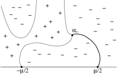
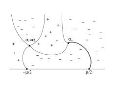
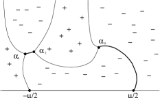
Figure 2. Left: Zero level curves of $\Im h^{0}$, pre-break. Center: Zero level curves of $\Im h^{0}$; this is a breaking point in the transition from genus zero to two; Notice the appearance of the double point. Right: Zero level curves of $\Im h^{2}$, post-break

2) In the case of the box potential, the double point $z_{0}\in{\mathbb{R}}$ and, therefore, the genus changes from zero to one ([17]).

We are now interested in the properties of the characteristic velocities at a double point $z_{0}$. Direct calculations ([30]) show that the Jacobian

(8.2) $$\frac{(\partial h^{N}_{z},\partial\Im h^{N})}{(\partial z_{0},\partial t)}=|h^{N}_{zz}(z_{0})|^{2}\Im h^{N}_{t}(z_{0}).$$

If $(x_{b},t_{b})$ is a the regular breaking point, then $h^{N}_{zz}(z_{0})\neq 0$. Let $z_{0}\not\in{\mathbb{R}}$. In this case it was proven in [29] that $|\Im h^{N}_{t}(z_{0})|+|\Im h^{N}_{x}(z_{0})|\neq 0$. Thus, either the Jacobian $\frac{(\partial h^{N}_{z},\partial\Im h^{N})}{(\partial z_{0},\partial t)}$ or $\frac{(\partial h^{N}_{z},\partial\Im h^{N})}{(\partial z_{0},\partial x)}$ is nonzero at $z_{0}$. Without any loss of generality, we can assume that the Jacobian (8.2) is nonzero at $z_{0}$. Then, there exists a unique breaking curve $t=t(x)$ passing through $(x_{b},t_{b})$ and a unique curve $z_{0}(x)$ passing through $z_{0}$ at $x=x_{b}$. Then, differentiating (8.1) along $t(x),z_{0}(x)$, we obtain

(8.3) $$\Im\left(h^{N}_{x}+h^{N}_{t}\frac{dt}{dx}\right)=0,~{}~{}~{}\qquad~{}~{}h^{N}_{zz}\frac{dz_{0}}{dx}+h^{N}_{xz}+h^{N}_{tz}\frac{dt}{dx}=0.$$

Thus, the slope $\frac{dt}{dx}$ of the breaking curve at $x_{b}$ and the velocity

(8.4) $$V=\frac{h^{N}_{tz}}{h^{N}_{xz}}=\frac{dq^{N}}{dp^{N}}$$

of the double point $z_{0}$ are are given by

(8.5) $$\frac{dt}{dx}=-\frac{\Im h^{N}_{x}}{\Im h^{N}_{t}},~{}~{}~{}\qquad~{}~{}~{}V=-\frac{\frac{h^{N}_{zz}}{h^{N}_{xz}}\cdot\frac{dz_{0}}{dx}+1}{dt/dx}\qquad{\rm or}\qquad\frac{dt}{dx}=-\frac{\Im p^{N}}{\Im q^{N}},~{}~{}~{}\qquad~{}~{}~{}V=-\frac{\frac{h^{N}_{zz}dz}{dp^{N}}\cdot\frac{dz_{0}}{dx}+1}{dt/dx}.$$

In the case $z_{0}\in{\mathbb{R}}$, according to (8.1), $h^{N}(z)$ does not have a jump at $z_{0}\in{\mathbb{R}}$. Thus, it is natural to consider the case when $h^{N}(z)$ is analytic in a neighborhood of $z_{0}$. Then, $\Im h^{N}\equiv 0$ on ${\mathbb{R}}$ near $z_{0}$, and the second condition in (8.1) becomes trivial. But then, if zero level curves of $\Im h^{N}$ are pinching ${\mathbb{R}}$ at $z_{0}$, we have six level curves of $\Im h^{N}=0$ emanating from $z_{0}$. Thus, we obtain new breaking curve conditions

(8.6) $$h^{N}_{z}(z_{0})=0~{}~{}\qquad~{}~{}{\rm and}~{}~{}\qquad~{}h^{N}_{zz}(z_{0})=0,$$

which imply

(8.7) $$V=-\frac{dx}{dt},~{}~{}~{}~{}~{}~{}\qquad\frac{dt}{dx}=-\frac{h^{N}_{zzz}\frac{dz_{0}}{dx}+h^{N}_{zzx}}{h^{N}_{zzt}}.$$

Thus, a real double point has a real velocity.

Examples 8.2.

1) In the transition from genus zero (with a movable branchpoint $\alpha=a+ib$) to a higher genus, the velocity $V$ of the double point $z_{0}$, according to (4.10), is given by $V=2z_{0}+\frac{b^{2}}{z_{0}-a}$, Using the large $t$ asymptotics of $z_{0}$ and of the breaking curve from [31], we can show that in the case “sech” potential, of $V\not\in{\mathbb{R}}$.

2) In the case of “box” potential, see Examples 3.1, the double point $z_{0}\in{\mathbb{R}}$. The first equation in (8.6) becomes

(8.8) $$4tz_{0}^{2}+2(x-L)z_{0}+2tq^{2}=0,$$

whereas the second equation in (8.6) means that the discriminant of (8.6) is zero. Thus we obtain the breaking curve (see [17], [10])

(8.9) $$\frac{L-x}{t}=2\sqrt{2}q\qquad{\rm and~{}the~{}double~{}point}\qquad z_{0}=\frac{q}{\sqrt{2}}.$$

Notice that the double point is stationary. Further direct calculations yield $h^{0}_{zt}=-\frac{4z^{2}}{\nu(z)}$, $h^{0}_{zx}=-\frac{2z}{\nu(z)}$, so that, according to (8.4), $V=\sqrt{2}q$.

We now want to prove that if $\alpha_{j}$ approaches a double point $z_{0}$ then $V_{j}$ approaches the velocity $V$ of $z_{0}$. Indeed, meromorphic differentials $dp,dq$ on the Riemann surface $\mathcal{R}$ of genus $m\in{\mathbb{N}}$ with poles at $\infty^{\pm}$ given by (6.30) can be written as

(8.10) $$dp=\frac{P(z)}{R(z)}dz,~{}~{}~{}~{}dq=\frac{Q(z)}{R(z)}dz$$

where $P=P(z;\vec{\alpha}),~{}Q=Q(z;\vec{\alpha})$ are polynomials of degrees $m+1$ and $m+2$ respectively, where $\vec{\alpha}\in{\mathbb{C}}^{2m+2}$ denotes the set of $2m+2$ distinct branchpoints of $\mathcal{R}$. Let $\vec{\alpha}\rightarrow\vec{\beta}$, where $\vec{\beta}\in{\mathbb{C}}^{2m+2}$ denotes the set $\vec{\alpha}$ after several pairs of branchpoints collided into the corresponding double points (more complicated clustering is also allowed) forming a singular Riemann surface, whose desingularization we denote by $\mathcal{R}_{0}$. It was proven in [2] that Boutroux deformations of $dp,dq$ are continuous in $\vec{\alpha}\in{\mathbb{C}}^{2N+2}$ and

(8.11) $$\lim_{\vec{\alpha}\rightarrow\vec{\beta}}P(z;\vec{\alpha})=\prod_{j}(z-z_{j})P_{0}(z;\vec{\beta}),\qquad\lim_{\vec{\alpha}\rightarrow\vec{\beta}}Q(z;\vec{\alpha})=\prod_{j}(z-z_{j})Q_{0}(z;\vec{\beta}),$$

where $dp_{0}=\frac{P_{0}(z;\vec{\beta})}{R_{0}(z)}dz$, $dq_{0}=\frac{Q_{0}(z;\vec{\beta})}{R_{0}(z)}dz$ are continuous limits of $dp,dq$ on $\mathcal{R}_{0}$, which is the Riemann surface for the radical $R_{0}$, $P_{0},Q_{0}$ are the corresponding polynomials and the product goes over all the double points $z_{j}$. Then, according to (8.10), (8.11),

(8.12) $$\lim_{\alpha_{j}\rightarrow z_{0}}V_{j}=\left.\lim_{\alpha_{j}\rightarrow z_{0}}\frac{dq}{dp}\right|_{\alpha_{j}}=\lim_{\alpha_{j}\rightarrow z_{0}}\frac{Q(\alpha_{j};\vec{\alpha})}{P(\alpha_{j};\vec{\alpha})}=\frac{P_{0}(z_{0};\vec{\beta})}{Q_{0}(z_{0};\vec{\beta})}=\left.\frac{dq_{0}}{dp_{0}}\right|_{z_{0}},$$

the latter being the velocity of the double point $z_{0}$.

Acknowledgements The work was supported in part by the Banff International Research Station, University of British Columbia, Vancouver, Canada. The work of the first author was supported in part by London Mathematical Society. The work of the second author was supported in part by the Department of Mathematics, University of Central Florida, Orlando, FL 32816-1364.

References

[1] E.D. Belokolos, A.I. Bobenko, V.Z. Enol’skii, A.R. Its and V.B. Matveev,
Algebro-Geometric Approach to Nonlinear Integrable Equations
Berlin etc., Springer-Verlag, 1994
[2] M. Bertola and A. Tovbis.
Meromorphic differentials with imaginary periods on degenerating
hyperelliptic curves.
Analysis and Mathematical Physics, 5(1):1–22, 2015.
[3] J.C. Bronski and J. N. Kutz, Numerical simulation of the semi-classical limit
of the focusing nonlinear Schrödinger equation, Phys. Lett. A 254 (1999) 325 -336
[4] H.D. Ceniceros and F.-R. Tian, A numerical study of the semi-classical limit of the focusing
nonlinear Schrödinger equation, Phys. Lett. A 306 (2002) 25 - 34.
[5] P. Deift, S. Venakides and X. Zhou
New Results in the Small-Dispersion
KdV by an Extension of the Method of Steepest
Descent for Riemann-Hilbert Problems, IMRN, 6, 285-299, 1997.
[6]
B.A. Dubrovin and S.P. Novikov,
Hydrodynamics of weakly deformed soliton lattices. Differential geometry and Hamiltonian theory.
Russian Math. Surveys, 44, 35-124, 1989.
[7] G.A. El, A.V. Gurevich, V.V. Khodorovskii and A.L. Krylov,
Modulational instability and formation of a nonlinear oscillatory structure in a focusing medium,
Phys Lett A, 177, 357-361, 1993.
[8] G.A. El,
Generating function of the Whitham-KdV hierarchy and effective solution of the Cauchy problem,
Phys. Lett. A., 222, 393-399 1996.
[9] G.A. El, A.L. Krylov and S. Venakides,
Unified approach to KdV modulations,
Commun. Pure Appl. Math. 54, 1243-1270 2001.
[10]
G.A. El,
E.G. Khamis and A. Tovbis.
Dam break problem for the focusing nonlinear Schrödinger equation and the generation of rogue waves.
arXiv:1505.01785. (2015)
[11] G.A. El and M.A. Hoefer, Dispersive shock waves and modulation theory,
arXiv:1602.06163 (2016)
[12] T. Grava and F.-R. Tian, The generation, propagation, and extinction
of multiphases in the KdV zero-dispersion limit, Comm. Pure Appl. Math. 55, (2002) 1569-1639.
[13]
A. V. Gurevich, L. P. Pitaevskii, Nonstationary structure of a collisionless
shock wave, Sov. Phys. JETP 38, (1974) 291–297.
[14] H. Flaschka, G. Forest and D.W. McLaughlin,
Multiphase averaging and the inverse spectral solutions of the Korteweg – de Vries equation,
Comm. Pure Appl. Math. 33, 739-784, 1980.
[15] M.G. Forest and J.E. Lee.
Geometry and modulation theory for periodic nonlinear Schrödinger equation,
in Oscillation Theory,
Computation, and Methods of Compensated Compactness, Eds. C. Dafermos et al,
IMA Volumes on Mathematics and its Applications 2,
Springer, N.Y., 1987.
[16] M. Hoefer and M. Ablowitz,
Dispersive shock waves.
Scholarpedia, 4(11) 5562, 2009.
[17] R. Jenkins, K. D. T.-R. McLaughlin.
The semiclassical limit of focusing NLS for a family of square barrier initial data.
Comm. Pure Appl. Math., 67 246–320, 2014.
[18] R. Jenkins and A. Tovbis.
Generation of multiphase waves from a barrier potential in the
semiclassical limit of the focusing nonlinear Schrödinger equation.
In preparation
[19]
S. Kamvissis, K. D. T.-R. McLaughlin, and P. D. Miller.
Semiclassical soliton ensembles for the focusing nonlinear
Schrödinger equation, volume 154 of Annals of Mathematics Studies.
Princeton University Press, Princeton, NJ, 2003.
[20] A.M. Kamchatnov,
New approach to periodic solutions of integrable equations and nonlinear theory of modulational instability.
Phys. Rep. 286, 199-270, 1997.
[21] P.D. Lax,
Periodic solutions of the KdV equation,
Comm. Pure Appl. Math., 28, 141 - 188, 1975.
[22]
P. D. Lax, C. D. Levermore,
The small dispersion limit of the Korteweg-de
Vries equation: 1-3,
Comm. Pure Appl. Math. 36, 253–290;
571–593; 809–830, 1983.
[23]
P. D. Lax, C. D. Levermore, S. Venakides,
The generation and propagation of
oscillations in dispersive initial value problems and their limiting
behavior, in: A. Focas, V. E. Zakharov (Eds.), Important Developments in
Soliton Theory,
Springer, Berlin, 205–241, 1994.
[24]
J. C. Luke,
A perturbation method for nonlinear dispersive wave problems,
Proc. Roy Soc. A. 292 403–412 1966.
[25] G. Lyng and P. Miller, The -soliton of the focusing nonlinear Schrödinger equation
for large, CPAM 60, 951-1026, 2006.
[26] S.P. Novikov,
The periodic problem for the Korteweg - de Vries equation. I.
Funktsional. Anal. i Prilozhen. 8 54 - 56, 1974.
[27] M.V. Pavlov,
Nonlinear Schrödinger equation and the Bogolyubov-Whitham method of averaging,
Theor. Math. Phys. 71, 351 1987.
[28]
A. Tovbis and S. Venakides.
Determinant form of the complex phase function of the steepest descent analysis of Riemann-Hilbert
problems and its application to the focusing Nonlinear Schrödinger equation.
Int. Math. Res. Not., rnp011, 2056–2080, 2009.
[29]
A. Tovbis and S. Venakides,
Nonlinear steepest descent asymptotics for semiclassical
limit of integrable systems: Continuation in the parameter space.
Comm. Math. Phys., 295(1), 139–160, 2010.
[30]
A. Tovbis, S. Venakides, and X. Zhou.
On semiclassical (zero dispersion limit) solutions of the focusing
nonlinear Schrödinger equation.
Comm. Pure Appl. Math., 57(7), 877–985, 2004.
[31]
A. Tovbis, S. Venakides, and X. Zhou.
On long time behavior of semiclassical (zero dispersion) limit of the focusing Nonlinear
Schroedinger Equation: Pure radiation case,
Comm. Pure Appl. Math., 59, 1379-1432, 2006.
[32] S.P. Tsarev,
On Poisson brackets and one-dimensional systems of hydrodynamic type,
Soviet Math. Dokl. 31, 488 1985.
[33]
S. Venakides,
The zero-dispersion limit of the Korteweg-de Vries equation
with non-trivial reflection coefficient,
Comm. Pure Appl. Math., 38
125–155 1985.
[34]
S. Venakides,
The Korteweg-de Vries equation with small dispersion: higher
order Lax-Levermore theory,
Comm. Pure Appl. Math.
43 335–361, 1990.
[36]
G.B. Whitham,
A general approach to linear and non-linear dispersive waves
using a Lagrangian,
Journal of Fluid Mechanics, 22 273–283 1965.
[37] G.B. Whitham,
Linear and Nonlinear Waves.
Wiley–Interscience, New York, 1974.
[38]
V. E. Zaharov and A. B. Šabat.
Integration of the nonlinear equations of mathematical physics by the
method of the inverse scattering problem. II.
Funktsional. Anal. i Prilozhen., 13(3):13–22, 1979.
[39]
X. Zhou,
Zakharov-Shabat inverse scattering.
In Scattering and inverse scattering in pure and applied science,
pages 1707–1716. Academic Press, London, 2002.