Measuring logic complexity can guide pattern discovery
in empirical systems

Abstract

We explore a definition of complexity based on logic functions, which are widely used as compact descriptions of rules in diverse fields of contemporary science. Detailed numerical analysis shows that (i) logic complexity is effective in discriminating between classes of functions commonly employed in modelling contexts; (ii) it extends the notion of canalisation, used in the study of genetic regulation, to a more general and detailed measure; (iii) it is tightly linked to the resilience of a function’s output to noise affecting its inputs. We demonstrate its utility by measuring it in empirical data on gene regulation, digital circuitry, and propositional calculus. Logic complexity is exceptionally low in these systems. The asymmetry between “on” and “off” states in the data correlates with the complexity in a non-null way; a model of random Boolean networks clarifies this trend and indicates a common hierarchical architecture in the three systems.

1 Introduction

Irreducibility is a property often ascribed to complex entities: their behaviour can not be compressed into compact descriptions. Symmetries — a paramount concept in physics — and recurrent patterns are prominent facilitators, enabling implicit definitions of the systems. The amount of implicitness allowed is a measure of information content [1], as illustrated by Kolmogorov’s definition of complexity. The concept of complexity pervades contemporary science, from the statistical mechanics of disordered systems and complex networks to economical and technological studies, prominently in the emerging field of complex systems, where it can promote the discovery of regularities and large-scale trends [2, 3, 4, 5, 6, 7, 8, 9, 10]. A recurrent question, notably in evolutionary biology, is whether complexity contributes to fitness [11, 12, 13, 14]. Its deep interplay with system-level properties such as tolerance and modularity has been investigated both in technological and biological designs [15, 16]; robustness of complex systems against fluctuations and attacks, in particular, is the subject of numerous studies [17, 18, 19].

Although complexity has been examined in detail in single contexts, by employing specific definitions, a study across disciplines is still lacking, and the general consequences and relations with other traits are still largely unknown. In this work we employ a definition of complexity based on Boolean logic [20], that is generic enough to be applicable in diverse fields. Logic functions are a natural and simple representation of how information flows in complex systems [21]. They are used to express genotype to phenotype mappings — both in metabolic [22] and electronic [23] systems —, rules for the control of gene expression [24], relations in protein networks [25], cryptographic cyphers [26], functions realised by digital electronic circuits [27], simple cooperative games [28], and they lie at the foundations of mathematical logic [29]. Complexity in a Boolean setting has been addressed especially regarding the global dynamics of Boolean networks [30], yet it proves profitable already to focus on single functions (nodes) [31, 32, 33]. We will concentrate on the properties of individual functions in this paper.

There are $2^{2^{n}}$ distinct Boolean functions with $n$ variables: finding useful coordinates in this high-dimensional space is a necessity in all fields concerned with logic functions. A large number of quantities describing various characteristics have been defined and analysed. Some are especially useful for assessing their cryptographic properties (such as correlation immunity [26]), some are suited for biological systems (such as the canalising quality [24]), some are designed to address issues in specific domains (such as the Nakamura number in cooperative game theory [34]). Here we concentrate on two natural and general “observables”, bias and complexity, whose versatility enables their use as a reference frame for comparing different systems in different fields.

We define the notion of logic complexity of a Boolean function as the size of the most compact Boolean expression that realises it [20] (see Sec. 2 for the choice of the description language). Firstly (in Sec. 3), we show that this definition assigns quantitatively different complexities to popular classes of logic functions. We clarify its relation with bias — a measure of the asymmetry between “on” and “off” values — and with resilience of the functions in noisy environments, thus establishing a quantitative relation between complexity and robustness. Importantly, logic complexity realises a rigorous and general measure for the notion of canalisation, a fruitful concept developed in the context of gene regulation [24]. In this field, our results further expose the inconveniences of the commonly used threshold functions, which turn out to have exceptionally high complexity.

Secondly (in Sec. 4), as an illustrative application of the concepts developed, we compute the complexity and the bias in three exemplary systems belonging to the realms of biology, technology, and mathematics, namely genetic regulation, electronic circuits, and propositional calculus. We find that the three systems are characterised by different ranges of the bias, and that the logic complexities are generally small, compared to a null model of random Boolean functions. The non-null trends are elucidated by a model of random Boolean networks, suggesting hierarchical organisation as a shared architecture.

Altogether, the results presented here advocate the use of bias and complexity as coordinates in a “morphospace” for the classification of logic functions, and in particular as a powerful tool for comparing Boolean models and data. More in general, our results remark that complexity is a measurable and empirically relevant trait, indicating similar features in dissimilar systems; however, its role is entangled with other important properties, such as bias, robustness, and information dispatching, and can not be contemplated in isolation.

2 Measuring logic complexity and bias

A Boolean (or logic) function maps the set $\{0,1\}^{n}$ to $\{0,1\}$, associating a truth value to each combination of its $n$ Boolean inputs (by convention the integers 1 and 0 mean true and false, or on and off, respectively). The binary nature of this description is sometimes just an approximation to a continuous or multi-valued empirical situation (such as the expression levels of a gene), but has the advantage of being simple to deal with. Since the domain is finite, a function can be specified by exhaustively listing the values it takes for all input combinations. Such a list constitutes the truth table of the function. See Fig. 1 for an example.

Figure 1: A Boolean function $f$ of $n=3$ literals $p,q,r$ has $8$ possible input combinations; the value of $f(p,q,r)$ on each of these (its truth table) completely specifies the function. The fraction of combinations on which $f$ is true, in this case 6 out of 8, is the bias $B$. The full disjunctive normal form of $f$ is obtained by explicitly stating all these combinations; in this example it would be $(\neg p\wedge\neg q\wedge\neg r)\vee(\neg p\wedge\neg q\wedge r)\vee(\neg p\wedge q\wedge r)\vee(p\wedge\neg q\wedge\neg r)\vee(p\wedge\neg q\wedge r)\vee(p\wedge q\wedge r)$. However a shorter form can be obtained by dividing the support of $f$ into cells, thus exploiting its symmetries. In this case $2$ cells (blue and red groupings) are sufficient (and necessary), thus the complexity is $C=2/8$.

The bias $B$, defined as the average output value over all input combinations, measures the propensity of the system described by the given function to be in one of the two states 0 and 1: $B=1$ for a tautology (the function that is true for all values of its inputs), $B=0$ for a falsity (the negation of a tautology).

Beyond the truth table, there is a way of writing Boolean functions which makes them more intelligible to humans, as opposed to computers. In fact, one can assign names to the function’s inputs — the literals — and decompose the function into binary sub-functions (i.e., functions of two literals) and negations (which are unary functions), thus writing it in the form of a Boolean expression; Fig. 1 presents an example. Such an expression contains the literals (possibly repeated), parentheses, and binary and unary operators. All Boolean functions can be expressed in this way, as every Boolean function can be written as the composition of binary and unary functions. We will use the set of logical operators $\{\land,\lor,\lnot\}$ (i.e., AND, OR, and NOT) to express them. As an example, consider the function of $3$ literals $p,q$, and $r$ that is true if one or two literals are true, and false otherwise. With our choice of basic operators it can be written as $(p\lor q\lor r)\land\lnot(p\land q\land r)$.

The definition of complexity that we shall employ for Boolean functions uses disjunctive normal forms (DNF) as the description language. A formula is in DNF if it is of the form $(A\land B\land\cdots)\lor(C\land D\land\cdots)\lor\cdots$, where $A,B,\ldots$ are literals or their negations. For example, $(p\land q)\lor\lnot p$ is in disjunctive normal form, while $\lnot(p\lor q)$ is not. Consider the tautology of $n=2$ literals. A particular normal form (called full DNF) can be built by listing explicitly all these combinations, thus obtaining the formula $(p\land q)\lor(p\land\lnot q)\lor(\lnot p\land q)\lor(\lnot p\land\lnot q)$; however, a more concise formula would be, for instance, $p\lor\lnot p$. Such a level of conciseness is intuitively related to the lack of complexity of the tautology. In general one expects that the more complex a function is, the less compact it can be made. We shall then define the complexity $C$ of a function as the number of terms in the shortest DNF specifying the function (normalised by $2^{n}$). This definition assigns minimum complexity to tautologies and their negations. At the other end of the spectrum, the parity function, which counts the number of true literals modulo 2, is balanced — meaning that $B=1/2$ — and has the largest possible complexity, namely $1/2$. Note that in general $C\leq B$. The main definitions and concepts are summarised in Fig. 1 for a simple function. See the Appendix for detailed definitions.

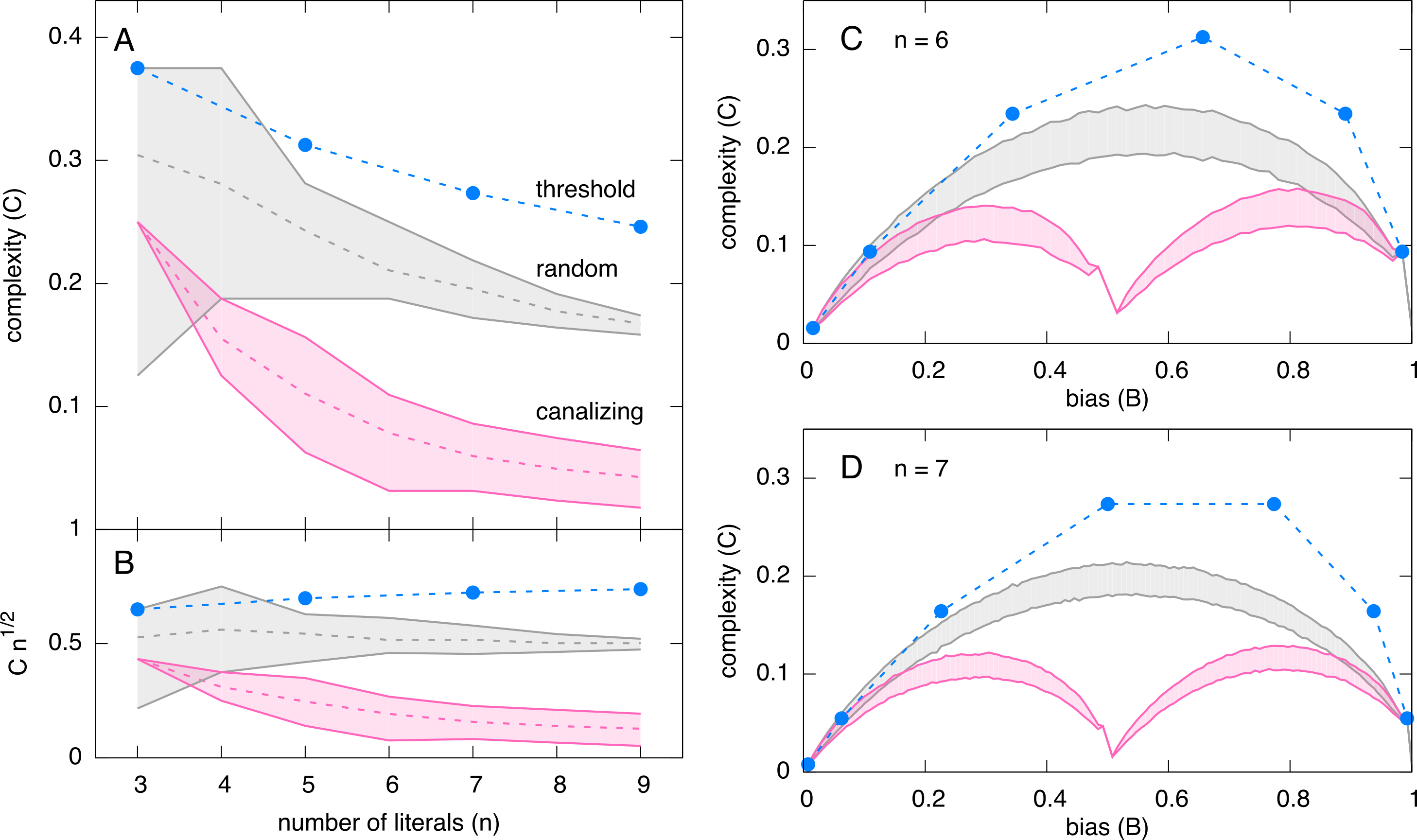
Figure 2: Commonly-used classes of functions are characterized by markedly different complexities. Threshold functions are more complex than the typical functions, while canalizing functions are simpler. Shaded areas are the $80\%$ variability intervals (at fixed bias) for each class. (A) Complexity as a function of the number of literals. Bias is restricted to the interval $(0.4,0.6)$ (there are no threshold functions of an even number of literals satisfying this constraint). (B) For random functions, $C$ decreases approximately as $1/\sqrt{n}$. The plot shows the rescaled quantity $C\sqrt{n}$. (C,D) Complexity as a function of bias for the three classes of functions considered, with $n=6$ and $n=7$ literals.

Measuring the bias of a function $f$ is straightforward, as it amounts to counting the number of ones in the truth table. Calculating the complexity, instead, is in general a computationally hard problem. The presence of symmetries in the truth table is what enables the compression. By symmetry, in this context, we mean a choice of a particular combination of values for a fixed subset of literals, such that the value of $f$, conditioned to this choice, does not depend on the other literals. This is the definition of a cell (see the Appendix). Finding the most compact normal form representing a function (or minimising it) thus amounts to finding the smallest number of cells sufficient to describe the function’s truth values; this means exploiting the set of its symmetries in the best possible way. However, even if one has listed all the cells of a function, there could be non-trivial overlaps between them — causing what is known as frustration in statistical mechanics — thus complicating the task of finding the smallest subset that recovers the function. In fact, this problem is equivalent to the “set cover problem”, a well-known NP-HARD problem in algorithmic complexity theory [35, 36].

Fortunately, since the minimisation of logic function is a crucial step in the design of digital circuits, standard algorithms are available for this task. Here we use an implementation of the Quine-McCluskey method [27], which deterministically finds the minimal form of a function. The maximum number of literals in the analyses presented here is $n=9$. For much larger functions, an approximate method is needed (such as “Espresso” [37]). Such methods have the advantage of being adapted to multi-valued logic, and they even allow for indeterminacies, so they can be used for computing logic complexity in more general settings.

We remark that ideas related to the one advanced here were proposed in the fields of unconventional computation and cellular automata [32, 33], where a notion of “conceptual representation” for Boolean rules was developed. That method, which makes use of a representation in terms of cells, essentially corresponds to the first step in the Quine-McCluskey algorithm, before the set-covering problem is solved.

3 Results

3.1 Bias and logic complexity discriminate popular classes of functions

We show here that the Boolean complexity takes values lying in different ranges for different commonly used classes of Boolean functions [38]. We examine random functions, i.e. Boolean functions with a fixed number of literals drawn with uniform probability, canalising functions, for which the value of a single input variable decides whether the other variables have any influence on the result, and threshold functions, for which the result is decided by the sum of “enhancer” variables minus the sum of “inhibitor” variables.

More formally, the ensemble of random functions with $n$ literals is defined as the set of all $n$-variables Boolean functions, endowed with the flat probability measure. This ensemble is useful as a null (unconstrained) model for discerning positive features in other classes of functions, as well as in the data. Random canalising functions are defined as follows. Consider a function $f(p_{1},\ldots,p_{n})$ of $n$ literals $p_{1},\ldots,p_{n}$. If $f$ is canalising, then by definition there exists a literal (by rearranging the literals, we can assume it is $p_{1}$) and two truth values (the input $I$ and the output $O$) such that $f(I,p_{2},\ldots,p_{n})=O$. If $p_{1}=\lnot I$, then $f(\lnot I,p_{2},\ldots,p_{n})=g(p_{2},\ldots,p_{n})$, where $g$ is a function of $n-1$ variables. The random canalising ensemble is specified by taking both $I$ and $O$ to be 0 or 1 independently with the same probability, and $g$ to be a random (uniform) function of $n-1$ literals. Threshold functions are often used to model regulatory rules starting from known molecular interactions (e.g., in the cell cycle of yeast [19, 39]). Let $a_{j}$ be a set of $n-1$ couplings, specifying the nature of the influence of a protein, identified by $j$, on a given gene product, identified by $i$. In particular, $a_{j}=1$ if $j$ is an enhancer and $a_{j}=-1$ if it is an inhibitor for $i$ (interaction strength can be taken into account by extending the possible values of $a_{j}$). If $x_{j}$ are on/off values specifying the presence ($1$) or absence ($0$) of each protein, then the Boolean state $f$ of $i$, is computed as $1$ or $0$ depending on the sign of $\sum_{j\neq i}a_{j}x_{j}-\theta$ (where $\theta$ is the threshold) with the exception that if the value is zero then $f=x_{i}$. The ensemble of random threshold functions of $n$ variables is defined by taking the $a_{j}$’s to be random independent Bernoulli variables in $\{-1,1\}$ (we will fix $\theta=0$, unless specified otherwise).

Figure 2A shows the complexities of the three classes of functions defined above, as the number of inputs $n$ is varied. For clarity, we excluded very unbalanced functions from this analysis, by restricting biases to the interval $0.4<B<0.6$. Threshold, canalizing, and random functions segregate into separate regions, already for $n\gtrsim 5$. Interestingly, the combination $Cn^{1/2}$ appears to be approximately increasing, decreasing, and constant in $n$ for the three classes respectively (Fig 2B).

Let us restrict the analysis to fixed numbers of literals $n$, in order to explore the relations between bias and complexity. Panels C and D in Fig. 2 show how the three classes occupy different regions in the B-C space. These plots have been obtained by generating random functions of each class for each possible value of $B$ fixed. While all types of functions have comparable complexities for extreme biases ($B\lesssim 0.2$ and $B\gtrsim 0.8$), in the balanced regime they are sharply discriminated by complexity. This rules out the possibility that the trends observed above might be due solely to how the typical biases $B$ depend on $n$ in the three classes of functions. Notice that both the bias and the complexity of threshold functions are quantised, because of symmetry under permutations of the variables. Perhaps surprisingly, their complexity is larger than the typical value. Changing the threshold value $\theta$ has the only effect of changing the ensemble weights of the functions (larger $\theta$ favours functions with lower bias), but the B-C plot remains the same.

The figure also exposes a non-monotonic correlation between complexity and bias, common to random and threshold functions. Canalising functions, whose definition modularly uses a random function of $n-1$ variables, present a similar behaviour on a halved scale; we are going to study this pattern more in detail.

3.2 Logic complexity realises a quantitative measure of canalisation

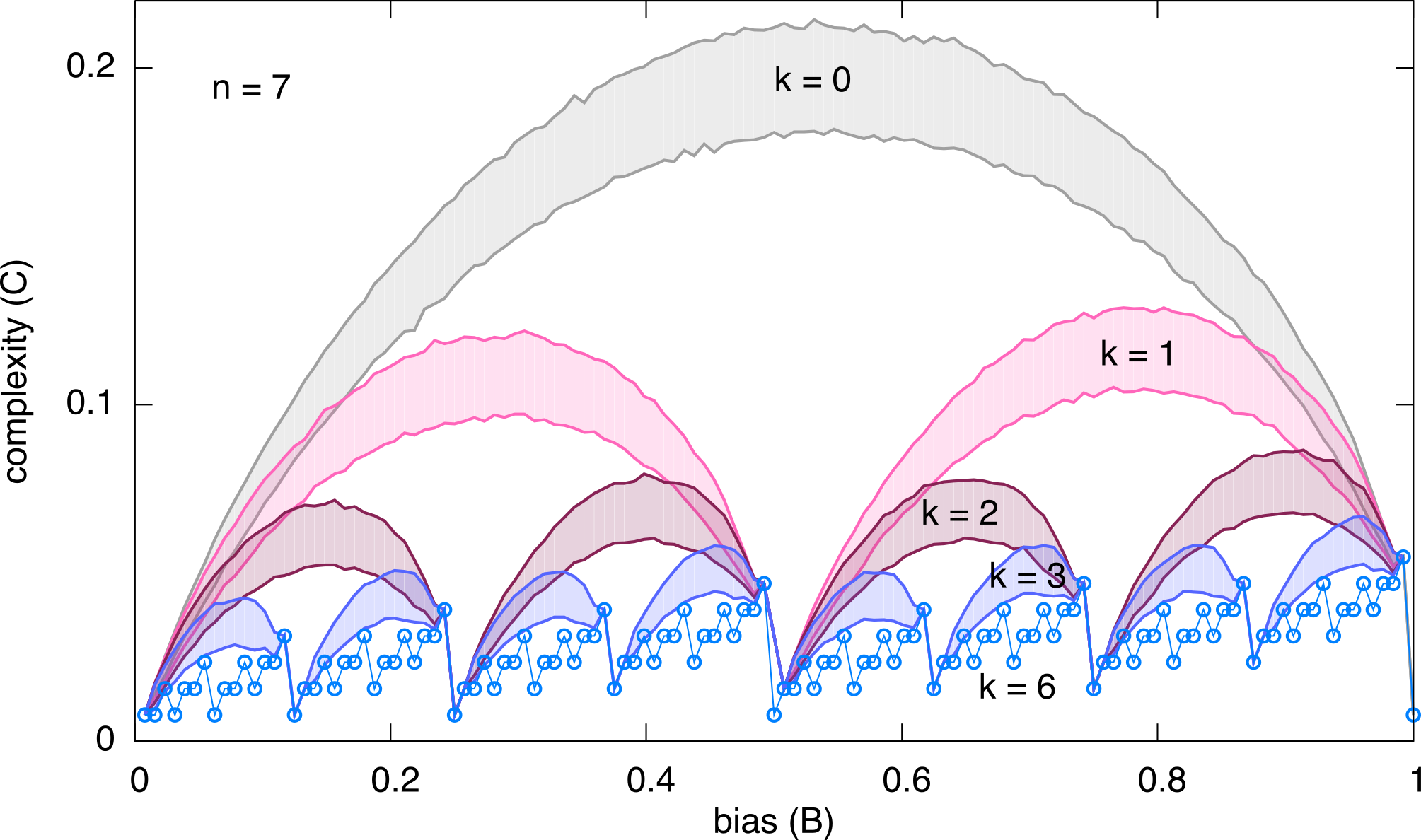
Figure 3: The complexity of random nested canalising functions decreases systematically with the level $k$. The shaded areas are the 80% variability intervals. The inverted-U pattern repeats itself $2^{k}$ times at level $k$. At level $n-1$ (lowermost curve) complexity is a deterministic function of bias (circles are the analytical expression given in the text). Here the number of input variables is $n=7$.

The definition of canalisation employed above isolates exactly one canalising variable $p_{1}$. However, a more general definition can be given, where the number of such special variables is $k<n$. If the value of the first canalising variable does not fix the output, then the second canalising variable is considered, and so on in a nested fashion, until the $k$-th variable. More precisely, given a set of input values $I_{1},\ldots,I_{k}$ and a set of output values $O_{1},\ldots,O_{k}$, $f(p_{1},\ldots,p_{n})$ takes the value $O_{j}$ if $p_{i}\neq I_{i}$ for all $i<j$ and $p_{j}=I_{j}$; otherwise it is a function $g(p_{k+1},\ldots,p_{n})$ of the remaining $n-k$ variables. The ensemble is specified by taking the $I_{i}$’s and $O_{i}$’s as random independent Bernoulli variables in $\{0,1\}$ and $g$ as a random function of $n-k$ literals. These functions will be called random nested canalising, and $k$ their level (our definition is based on that of nested canalisation given in [40], but it uses a less constrained measure).

We generated 1000 random nested canalising functions of level $k=1,\ldots,n-1$ for each possible value of their bias, and computed their complexity. The results (with $n=7$) are in Fig. 3 (not all levels are shown for clarity; other values of $n$ yield similar results). Disregarding for the moment the fine structure that appears as a function of bias, the overall trend is clear: the more levels of canalisation a function has, the smaller is its complexity. Canalisation itself can not be measured quantitatively: the level $k$ is a rough measure, but it takes only $n-1$ different values. Therefore, complexity, which can take $2^{n}$ different values, appears as a much more detailed measure of canalisation.

The fractal nature of the plot is interesting. At level $k$, the inverted-U pattern displayed by random functions is repeated $2^{k}$ times (this is true independently of $n$). Fully canalising functions, i.e. those at level $n-1$, satisfy a deterministic relation between bias and complexity, which can be seen to be given by $C=S_{2}(B2^{n})/2^{n}$, where $S_{q}(m)$ is the sum of all the digits in the base-$q$ representation of the integer $m$ (in the case $q=2$ it is known as the binary weight).

3.3 Logic complexity constrains robustness

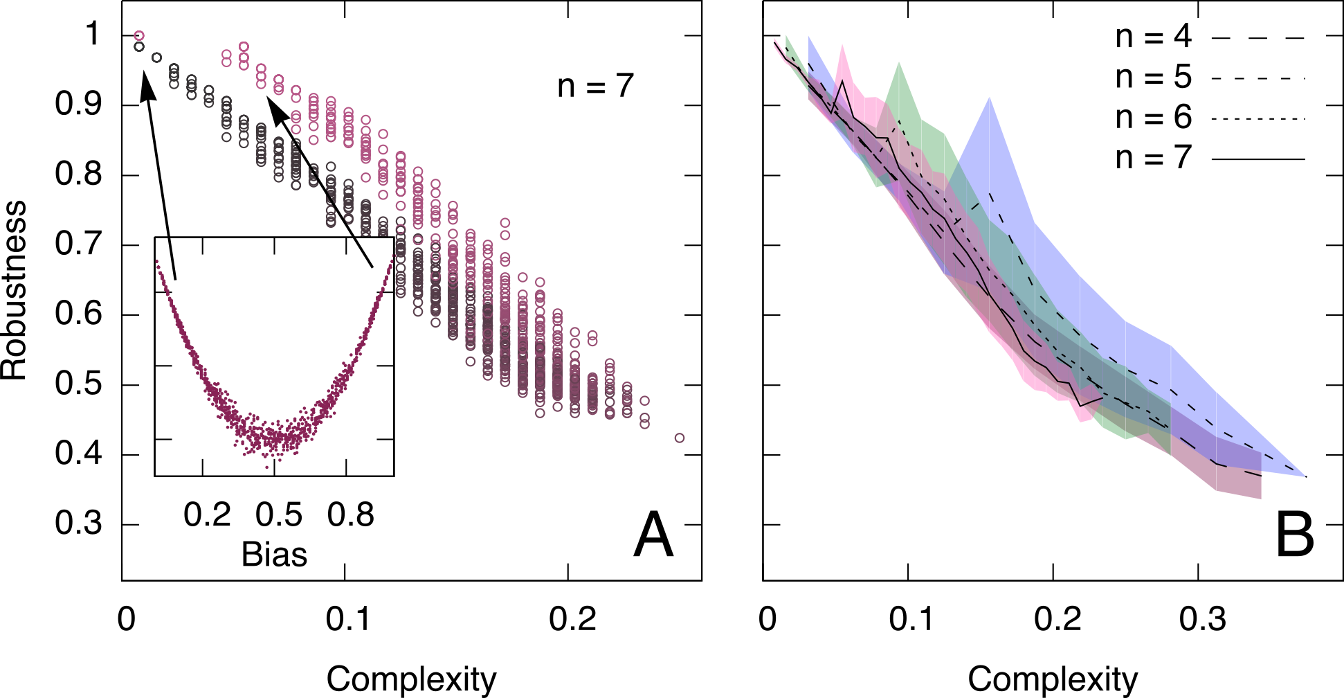
Figure 4: Complexity of a Boolean function ($x$ axis) strongly constrains its robustness ($y$ axis), while bias and number of variables have a weak influence. Points in panel A show the robustness versus the complexity of 1000 random Boolean functions with $n=7$ literals, generated uniformly on the full range of biases; the inset shows robustness versus bias for the same data. Panel B collects data for different numbers of literals, showing the average (lines) and the $80\%$ variability interval (shaded areas) of the robustness as functions of the complexity.

Noise is an important element of both living and artificial systems. Robustness against errors and fluctuations, for instance in protein folding or signal transduction, is a central question in biology [41, 42]. In the field of regulatory networks, noise can be implemented by means of a stochastic generalisation, called probabilistic Boolean networks [43], where the functions computed by nodes are subject to a certain degree of variability. One can then ask what noise level the system can sustain without disrupting its functions. Such questions are relevant in technological systems as well.

It is then interesting to discover that Boolean complexity is closely related to fault tolerance in our simple setting. We employ the definition of robustness $R$ detailed in the Appendix, which counts the fraction of single-variable flips that have no effect on the output. More precisely, it is equal to the probability that $f(p_{1},\ldots,p_{j},\ldots,p_{n})=f(p_{1},\ldots,\lnot p_{j},\ldots,p_{n})$, when the values of $p_{1},\ldots,p_{n}$ are chosen randomly and $j$ is a random integer between 1 and $n$. As discussed above, simple functions are intuitively recognised as those having a large number of symmetries, where a symmetry (as outlined by the technical notion of cell described in the Appendix) is a group of input combinations such that the function’s value is not sensitive to changes of some of the variables. Thus, one expects simpler functions to be more robust. In fact, computing the robustness for functions with varying biases and complexities shows that $R$ is strongly dependent on $C$ (and very slightly on $B$). Figure 4 displays these correlations, and shows that the dependence of $R$ on the number of variables $n$ is almost undetectable. Statistically significant correlations remain also if one conditions the analysis to fixed values of the bias, thus confirming the relation. Also, flipping $2$ variables instead of $1$, thus increasing the noise level in the definition of $R$, has negligible effects on the results.

4 Application to empirical systems

We are going to apply the concepts developed in the previous sections to empirical systems of different types, belonging to the broad areas of biology, technology and mathematics. In particular, we will focus on transcription regulation in Eukaryotes, digital electronic circuitry in a general-purpose processor, and theorems in propositional logic. The three data sets employed here are chosen as a reference, and do not intend to be general representatives of their respective fields. However, interesting features about how logic complexity is expressed in empirical systems can be isolated already from this limited exploration.

4.1 Data sets

Genetic regulation

Transcription regulation is the machinery by which a cell coordinates the generation of RNA from DNA, ultimately orchestrating the production of proteins in response to internal and external stimuli. Several proteins, including transcription factors that bind to the DNA, can participate in the regulation of a single gene. They can play the simple roles of activators and repressors of transcription, but their complex interactions within chromatin can generate complicated dependencies between their presence/absence patterns and the expression level of a given gene. These relationships can then be summarised by Boolean functions expressing whether each gene is transcribed or not, depending on the presence of each protein that has an influence on the gene. We compiled a small data set of 34 such functions, obtained from the literature (5 regulating flower morphogenesis in Arabidopsis thaliana [44]; 15 regarding segment polarity in Drosophila melanogaster [45]; 6 controlling the mammalian cell cycle [46]; 8 belonging to T lymphocytes in vertebrates [47, 48]). We restricted to papers where experimentally-validated functions were employed for the construction of Boolean-network representations of gene interactions, since these are the most easily accessible, and they have the additional benefit of being used already in a Boolean setting. We circumscribe the analysis to functions with $n=3,4,5,6,7$ inputs.

Digital circuits

Logic functions are the fundamental building blocks of digital electronics. As mentioned above, hardware engineering needs were the driving force behind the deployment of the known algorithms for minimising Boolean functions. Digital circuits are natively composed of logic gates, and therefore have a natural network representation which has been already investigated within a statistical physics viewpoint [49]. We used data from the ITC’99 benchmark [50], considering a partial logic-gate representation of the Intel 80386 processor (data set b15 [51]). The data are in the form of a graph where nodes are gates computing simple functions (either AND, NAND, OR, NOR, or NOT) of a small number of inputs, and links run from outputs to inputs of nodes. The full network has around 8000 nodes and 17000 links. We built individual functions by considering all sub-graphs with $n=3,4,5,6,7$ input links. The enumeration was restricted to sub-graphs with at most 5 hierarchical levels (i.e., the longest path from an input node to an output node travels along 4 links); the data were then pruned of functions corresponding to a single node. Our final data set comprises 1891 Boolean functions (approximately 250 for $n=3$, 170 for $n=4$, and 500 for $n=5$, $n=6$, and $n=7$).

Formal logic

The relations between logic functions and expressions constitute the branch of logic known as propositional calculus. Deductive systems can be used to formalise and check, solely from syntactic grounds, whether a given formula is a consequence of another. Basically, they rely on a set of axioms, that are true by definition, and a set of inference rules, that are used to form true expressions starting from true premises. The data set we use is based on the Metamath project [52]. which implements a standard deductive system for the formalisation of mathematics, providing a language and a proof-validation software to the community of people involved. We restricted to the part of the Metamath database that regards propositional calculus, for which one can interpret expressions as Boolean functions. It depends on only three axioms, (known as the principles of simplification, transposition, and Frege) and only one inference rule, the modus ponens. Theorems can be in either one of two forms. The first is $\vdash P$ — where $P$ is an expression — meaning “$P$ is provable in the formal system”, in which case $P$ is a tautology, thanks to the coherence of the system. The second is $\vdash Q_{1},\vdash Q_{2},\ldots,\vdash Q_{k}\Rightarrow\vdash R$, meaning “if all $Q_{i}$’s are provable in the system, than so is $R$”. Our data set was constructed as follows. If a theorem is in the second class, we keep the proposition $R$. If it is in the first class, it is trivially a tautology (maximum bias, minimum complexity), so we parse $P$ and cast it into the form $OP(Q,R)$, where OP is a binary operator; then if OP is a conditional ($Q\rightarrow R$) we keep $R$ (since the original theorem could have been written as $\vdash Q\Rightarrow\vdash R$), if OP is a biconditional ($Q\leftrightarrow R$) we keep both $Q$ and $R$, if OP is a disjunction ($Q\lor R$) we keep both $Q$ and $R$ (since it could have been written as $\vdash\lnot Q\Rightarrow\vdash R$ and $\vdash\lnot R\Rightarrow\vdash Q$). We end up with 327 propositions.

4.2 Empirical functions have low complexity

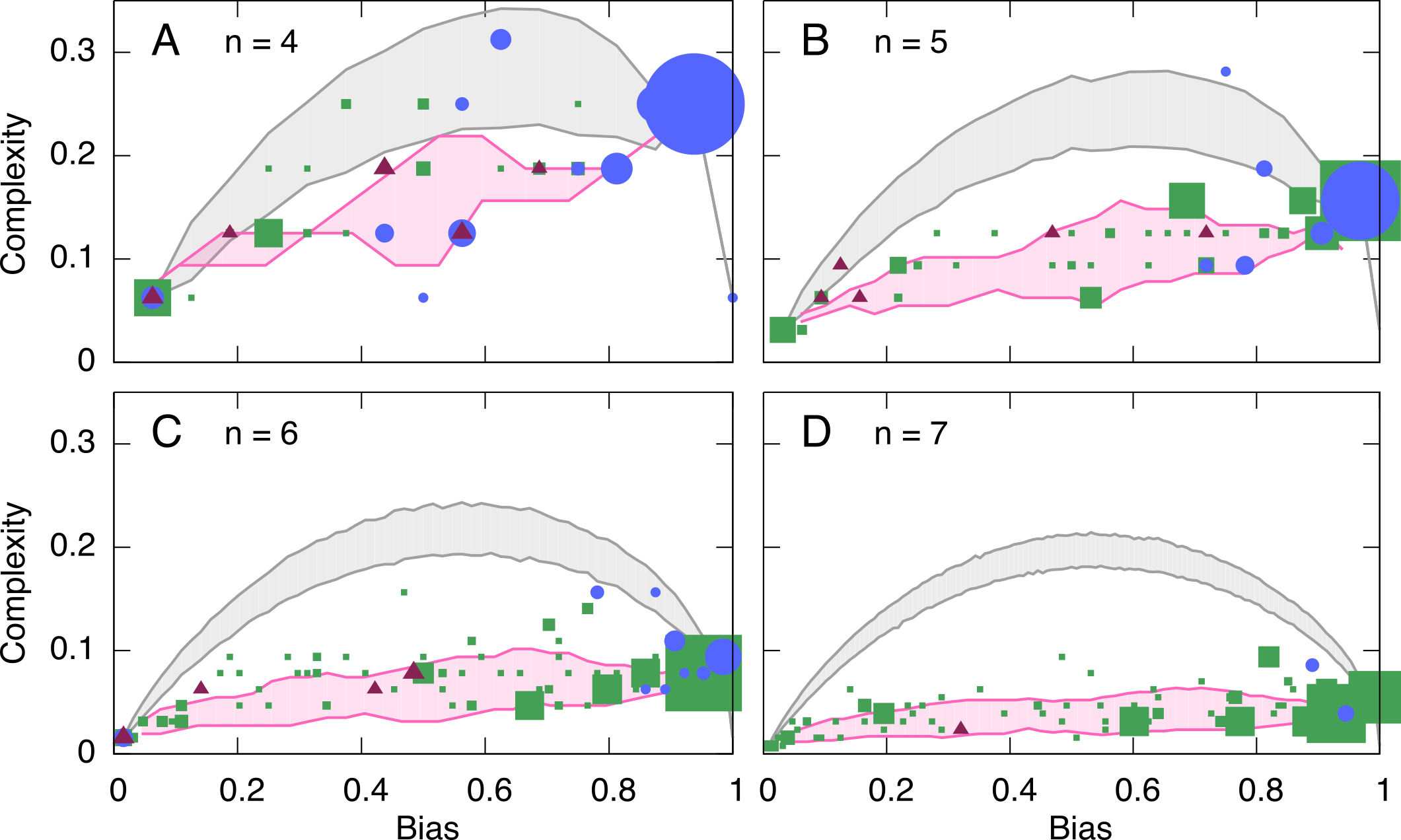
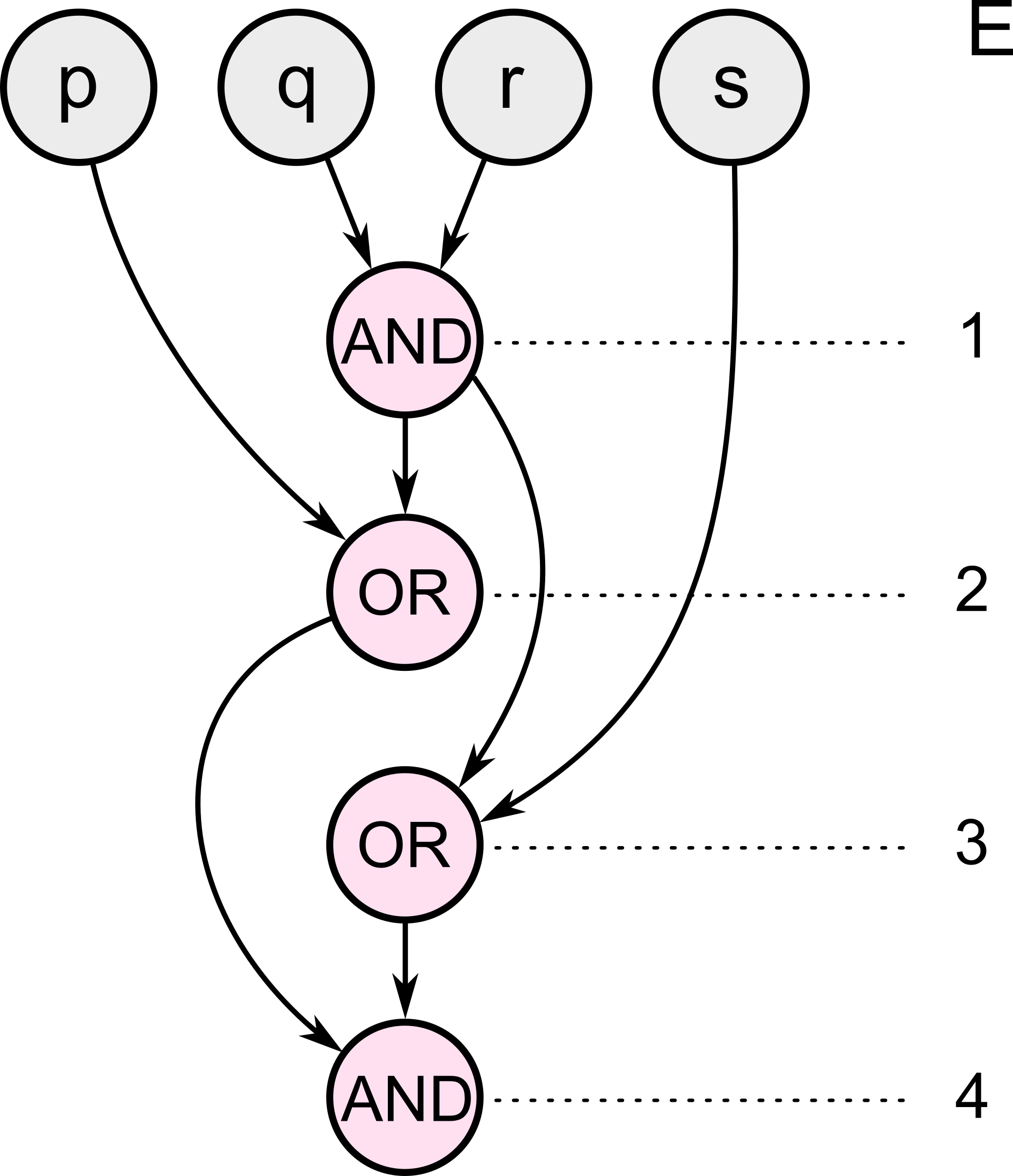
Figure 5: The bias (on $x$ axes) and the complexity (on $y$ axes) of logic functions from empirical data sets are related in a non-null way, which is captured by a model of random Boolean networks. (A,B,C,D) Functions defined by genetic regulatory circuits (red triangles), electronic sub-circuits in the i386 microprocessor (green squares), and theorems in propositional logic (blue circles) have lower complexity than typical Boolean functions, especially for larger numbers of literals. Grey shaded areas comprise $\sim 80\%$ of all functions with a given bias. Point sizes are proportional to the number of data points having the same bias and complexity. The pink shaded areas are small random Boolean networks, schematically described in panel (E). In this example, the network is built in four steps; the resulting function is given by the bottommost node (which is the first one that connects to all literals $p,q,r,s$), and is $(p\lor(p\land q))\land(s\lor(p\land q))$.

The values of bias and complexity for the function in our data sets are shown in Fig. 5A–D. The bias (on the horizontal axis) discriminates between the three systems, for each $n$ considered. Functions expressing gene-regulatory rules take the value $0$ (meaning “no gene transcript”) more often than in the other systems, while theorems in mathematical logic show an inclination for the value $1$ (meaning “true”); electronic sub-circuits, though more balanced, are slightly biased towards the “on” state, contrary to what one would expect from energy-consumption considerations. Comparison with the null model shows that the complexity of empirical functions is consistently lower than the typical Boolean functions, especially for larger $n$.

4.3 A random-network model reproduces the empirical trends

A noticeable feature of the empirical B-C plots is the monotonic correlation between bias and complexity, in spite of the non-monotonic one expected for random functions. This suggests the existence of a positive mechanism present either in the empirical systems themselves or in the way they are modelised through logic functions. We explore a possible scenario based on a model of random Boolean networks, defined below. Our goal is to show that analysis of empirical data by means of the bias-complexity coordinates can be helpful in discerning non-null features in the data and devising positive models.

Let us start with $n$ input nodes, which represent the literals (refer to Fig. 5E). We build a graph iteratively by adding nodes one by one. Each new node carries a random binary function $\phi$ (either OR or AND), and attaches itself to two randomly chosen nodes, among those already present (literals included). If the values of these nodes are $p$ and $q$, than the value of the new node will be $\phi(p,q)$. The growth process is stopped as soon as the first node depending on all $n$ input literals appears. More precisely, the function $f$ embodied by the network is defined as the first node whose light cone contains all input nodes, the light cone of a node $A$ being defined as the set of all nodes $B$ such that there is a directed path in the network going from $A$ to $B$. Figure 5 shows that the bias-complexity relation predicted by this model is in reasonable accord with the trend observed in the empirical systems. The most notable feature is the roughly linear correlation between the two coordinates, which is instead non-monotonic for random functions.

Notice that we have chosen $\phi$ to be either OR or AND with equal probability. This choice generates functions with biases covering the whole interval $(0,1)$; a statistical prevalence of OR reduces the average $B$, while the opposite happens for AND, without modifying the trend observed. Adding a negation (NOT) in front of randomly-chosen variables does not change the results appreciably.

5 Discussion

The view presented here is based on the observation that logic functions are a widespread tool in modelling complex systems, realising compact two-state descriptions of complicated response functions. Therefore, a definition of complexity in a Boolean setting is useful, as it enables the quantitative comparison of behaviours across systems. It proves fruitful also within fields, as a concise indicator summarising several “microscopic” features in a single global observable.

As we showed, complexity effectively discriminates different classes of functions widely used in modelling approaches. Specifically within the class of canalising functions, it produces a quantitative measure of “how much” canalisation is realised. This measure is more general and more detailed than the number of canalising variables; it can be measured exactly for all Boolean functions and is arguably more suited to information-theoretic analyses. A long-standing question in the field of genetic regulation concerns the properties of regulatory networks responsible for their not being chaotic [38, 53]. It is well known that Boolean networks can display chaotic dynamics in certain regimes, at variance with the ordered state their are found to be in living systems. Canalisation is one quality of regulatory rules that has been found to promote network stability. It would be interesting to investigate how the order-chaos transition in the Kauffman model (a random network of random Boolean functions [54]) depends on the complexity of the rules; the results regarding robustness described above are relevant in this sense (see also [33, 55, 40]). Another consequence of our results on the classes of functions commonly used for gene regulation is that threshold functions impose a systematic tendency towards high complexity, and constrain both bias and complexity to very specific values.

The relations uncovered between complexity, on/off asymmetry, and robustness seem to indicate the presence of architectural similarities between the empirical systems considered. In particular, the low Boolean complexity observed in our three data sets and the monotonic correlation between $C$ and $B$ suggest the existence of a positive mechanism underlying these empirical systems. A possible rationalisation is given by the simplified model of random logic networks described above, which reproduces the trends. The information provided is twofold. First, our example of an empirical application shows that measuring complexity, especially combined with bias in the B-C parametrisation, can promote the discovery of hidden regularities, trends, and tradeoffs. Second, it suggests a possible underlying mechanism recapitulating the statistical regularities measured, namely a modular structure where the whole function to be realised by the system is expressed by means of smaller functions (i.e., with fewer inputs than $n$) organised in a hierarchical arrangement. Such a common architecture need not be generated by common evolutionary processes in the three systems. It may be the consequence of selection — for instance favouring robustness —, or a neutral effect of the system’s organisation, or it could expose our preference for simple structures, at least in artificial systems. Remarkably, Boolean complexity of concepts has been found to be a predictor of subjective difficulty in human learning [56]. (In the case of regulation, the difficulty in performing the experiments and completely identifying the set of regulating proteins may be partially responsible for the low complexities observed.)

Finally, we remark that the results presented are not sensitive on the particular description language one employs in the definition of logic complexity. We used disjunctive normal forms (i.e., disjunctions of conjunctive clauses) throughout the paper, but we checked that definitions based on conjunctive normal forms (conjunctions of disjunctive clauses) or algebraic normal forms (exclusive disjunctions of conjunctive clauses) do not change our result statements.

Appendix

A Boolean function $f$ of $n$ variables is a map

$$\begin{split}f:\{0,1\}^{n}&\to\{0,1\}\\ \sigma&\mapsto f(\sigma)\end{split}$$

where $\sigma=\{p_{1},p_{2},\ldots,p_{n}\}$ is the configuration of the input variables (or literals) $p_{i}$. A logic function $f(p_{1},p_{2},\ldots,p_{n})$ is uniquely determined by its truth table, which is the explicit listing of the value of $f$ for all $2^{n}$ possible combinations of the $n$ variables $p_{i}$. Notable functions are the tautology, which takes the value 1 for all $\sigma$ (a tautology is “always true”), and the parity function $\pi(p_{1},\ldots,p_{n})=\sum p_{i}\;\mathrm{mod}\;2$, which takes the value 1 when the number of literals equal to 1 is odd (and 0 otherwise).

Boolean functions can be built by composition of “smaller” functions, e.g. a ternary function $f$ can be obtained starting from two binary functions $g$ and $h$ as $f(p,q,r):=g(p,h(q,r))$. This permits the definition of a small “vocabulary” of atomic functions, from which Boolean expressions, corresponding to larger functions, can be constructed by composition. As the basic building blocks for logic functions, we choose the two binary functions AND ($\land$) and OR ($\lor$), and the unary function NOT ($\lnot$). The set $\mathcal{B}=\left\{\land,\lor,\lnot\right\}$ is functionally complete, meaning that the three atomic functions can be composed to represent all possible functions of $n$ literals. Notice that $\mathcal{B}$ is not minimal, as both $\land$ and $\lor$ could be expressed by means of the other two connectives. However, it is a very natural generating set, as it is tightly linked to the representation of functions in terms of their truth table.

The two-dimensional morphospace we use summarises each function by two quantities: bias and complexity. Bias measures the average value taken by the function, and is therefore an indicator of the asymmetry between the “on” (1) and “off” (0) output states.

• The bias $B$ (or on/off asymmetry) of a Boolean function $f$ is the fraction of input combinations for which $f$ is true, namely

  $$B=\sum_{\{\sigma\}}f(\sigma)/\sum_{\{\sigma\}}1,$$

  where the sums are over all possible input combinations $\sigma$ (hence $\sum 1=2^{n}$ for a function of $n$ variables).

Defining complexity, as in Kolmogorov’s definition, requires the specification of a description language. A natural language for logic functions is that of disjunctive normal forms (DNF). As described in the text, these are Boolean expressions built with the elements of our base set $\mathcal{B}$, such that they take a canonical form, namely a disjunction of conjunctive clauses, in terms of literals and their negations. A DNF is said to be full if each literal appears exactly once in each conjunctive clause. If a logic function $f$ is expressed via its truth table, then its full DNF can be immediately constructed, simply by listing all combinations of truth values for which $f$ is true. For instance, the function XOR$(p,q)$, which is true if exactly one of its literals $p,q$ is true, can be written as $(p\land\lnot q)\lor(\lnot p\land q)$. Let us define the length $l(\varphi)$ of a DNF $\varphi$ as the number of clauses, i.e., the number of terms separated by $\lor$ operators). The bias of the function is then equal to the length of the full DNF. Each term in a DNF can be considered as an autonomous sub-function of a number $k$ of literals, defining a k-cell in the function’s truth table. A $k$-cell of a function is a subset of input combinations for which the function is true and such that it can be expressed, when restricted to those combinations, as a single conjunctive term $p_{1}\land p_{2}\land\ldots\land p_{k}$ (possibly with negations), all other $n-k$ literals remaining free.

The full disjunctive normal form is typically not a compact representation of a function. As an extreme case, consider the tautology of $n$ variables: its bias is $1$ and its full DNF has $2^{n}$ terms. However, a much shorter DNF is for instance $p\lor\lnot p$ (where $p$ is any literal), which is still in DNF and has length 2, thus defining the same function with a much shorter expression. As discussed in the text, complexity is expected to measure the minimal amount of information one has to specify when defining an entity. Having fixed DNFs as the natural language, it is then straightforward to define the complexity of a logic function as follows.

• Let us denote by $\Phi(f)$ the set of all the DNFs of the function $f$ (it is a finite set if repetitions of clauses are prohibited). The complexity $C$ of a Boolean function is the length of its shortest disjunctive normal form, normalised by the length of its truth table, namely

  $$C=\min_{\varphi\in\Phi(f)}l(\varphi)/\sum_{\{\sigma\}}1,$$

  where $\sigma$ is as in Definition 1.

An equivalent definition in terms of cells can be given, as the minimum number of cells needed to cover the set of input combinations for which the function is 1 (see e.g. [1]).

Since the full DNF belongs to $\Phi(f)$, and its length is the number of 1s in the truth table, the inequality $C\leq B$ holds in general. It is interesting to note that the parity function of $n$ variables, for which $B=1/2$, has the largest possible complexity, namely $C=1/2$ (the sequence of its values realises a fractal known as the Thue-Morse sequence). This is easily proved by noting that if there existed any cell containing more than one element, than it would contain at least two combinations of inputs having different parities. Parity functions are used in various contexts, due to their symmetry and tractability [31, 57].

Finally, the notion of robustness measures how much fluctuations in the input variables affect the function’s value.

• The robustness $R$ of a Boolean function $f$ is the fraction of pairs $\{\sigma_{1},\sigma_{2}\}$ such that $f(\sigma_{1})=f(\sigma_{2})$, where $\sigma_{1}$ and $\sigma_{2}$ are two combinations of inputs differing only in the value of one variable (i.e., their Hamming distance $|\sigma_{1}-\sigma_{2}|$ is 1), namely

  $$R=\sum_{|\sigma_{1}-\sigma_{2}|=1}\!\!\delta_{f(\sigma_{1}),f(\sigma_{2})}/\!\!\sum_{|\sigma_{1}-\sigma_{2}|=1}\!\!\!1$$

Tautologies and their negations have the highest robustness, namely $R=1$, as changing the value of any variable never changes the result. The parity function, on the contrary, has the lowest robustness, $R=0$, since by definition a single flip of any of its variables changes the function’s value. Remark that this definition of $R$ fixes a specific scale for the fluctuations, namely only $1$ variable. The analogous definition where one considers $2$ flips would assign minimum complexity to parity functions. However, the results presented in the text are unaffected by the number of variables flipped, showing that the relation between robustness and complexity is robust.

References

- [1] A. Carbone, S. Semmes, A Graphic Apology for Symmetry and Implicitness, Oxford mathematical monographs, Oxford University Press, 2000.
- [2] D. Stein, C. Newman, Spin Glasses and Complexity, Primers in Complex Systems, Princeton University Press, 2013.
- [3] A. Barrat, M. Barthlemy, A. Vespignani, Dynamical Processes on Complex Networks, 1st Edition, Cambridge University Press, New York, NY, USA, 2008.
- [4] C. A. Hidalgo, R. Hausmann, The building blocks of economic complexity, Proceedings of the National Academy of Sciences 106 (26) (2009) 10570–10575.
- [5] A. Tacchella, M. Cristelli, G. Caldarelli, A. Gabrielli, L. Pietronero, A new metrics for countries’ fitness and products’ complexity, Sci. Rep. 2.
- [6] G. Tononi, G. M. Edelman, Consciousness and complexity, Science 282 (5395) (1998) 1846–1851.
- [7] J. McNerney, J. D. Farmer, S. Redner, J. E. Trancik, Role of design complexity in technology improvement, Proceedings of the National Academy of Sciences 108 (22) (2011) 9008–9013.
- [8] K. Frenken, Technological innovation and complexity theory, Economics of Innovation and New Technology 15 (2) (2006) 137–155.
- [9] D. P. Feldman, J. P. Crutchfield, Measures of statistical complexity: Why?, Physics Letters A 238 (4–5) (1998) 244 – 252.
- [10] C. R. Shalizi, K. L. Shalizi, R. Haslinger, Quantifying self-organization with optimal predictors, Phys. Rev. Lett. 93 (2004) 118701.
- [11] J. E. Auerbach, J. C. Bongard, Environmental influence on the evolution of morphological complexity in machines, PLoS Comput Biol 10 (1) (2014) e1003399.
- [12] N. J. Joshi, G. Tononi, C. Koch, The minimal complexity of adapting agents increases with fitness, PLoS Comput Biol 9 (7) (2013) e1003111.
- [13] Z. Wang, B.-Y. Liao, J. Zhang, Genomic patterns of pleiotropy and the evolution of complexity, Proceedings of the National Academy of Sciences 107 (42) (2010) 18034–18039.
- [14] C. Adami, C. Ofria, T. C. Collier, Evolution of biological complexity, Proceedings of the National Academy of Sciences 97 (9) (2000) 4463–4468.
- [15] M. E. Csete, J. C. Doyle, Reverse engineering of biological complexity, Science 295 (5560) (2002) 1664–1669.
- [16] J. Carlson, J. Doyle, Complexity and robustness, Proceedings of the National Academy of Sciences 99 (suppl 1) (2002) 2538–2545.
- [17] R. Albert, H. Jeong, A.-L. Barabasi, Error and attack tolerance of complex networks, Nature 406 (6794) (2000) 378–382.
- [18] J. Macia, R. V. Solé, Distributed robustness in cellular networks: insights from synthetic evolved circuits, Journal of The Royal Society Interface 6 (33) (2009) 393–400.
- [19] F. Li, T. Long, Y. Lu, Q. Ouyang, C. Tang, The yeast cell-cycle network is robustly designed, Proceedings of the National Academy of Sciences of the United States of America 101 (14) (2004) 4781–4786.
- [20] I. Wegener, The Complexity of Boolean Functions, John Wiley & Sons, Inc., New York, NY, USA, 1987.
- [21] G. Tkačik, W. Bialek, Information processing in biological systems, Annu Rev Cond Matt Phys 7 (2016)
- [22] A. Barve, A. Wagner, A latent capacity for evolutionary innovation through exaptation in metabolic systems, Nature 500 (7461) (2013) 203–206.
- [23] R. V. Solé, S. Valverde, M. R. Casals, S. A. Kauffman, D. Farmer, N. Eldredge, The evolutionary ecology of technological innovations, Complexity 18 (4) (2013) 15–27.
- [24] S. E. Harris, B. K. Sawhill, A. Wuensche, S. Kauffman, A model of transcriptional regulatory networks based on biases in the observed regulation rules, Complexity 7 (4) (2002) 23–40.
- [25] P.M. Bowers, S.J. Cokus, D. Eisenberg, T.O. Yeates, Use of logic relationships to decipher protein network organization, Science 306 (2004) 2246–9.
- [26] C. Carlet, Boolean functions for cryptography and error-correcting codes, in: Y. Crama, P. L. Hammer (Eds.), Boolean Models and Methods in Mathematics, Computer Science, and Engineering, Cambridge University Press, 2010, pp. 257–397, cambridge Books Online.
- [27] G. D. Micheli, Synthesis and Optimization of Digital Circuits, 1st Edition, McGraw-Hill Higher Education, 1994.
- [28] J. Bilbao, Cooperative Games on Combinatorial Structures, Theory and Decision Library C, Springer US, 2000.
- [29] A. Church, Introduction to mathematical logic. vol. 1 (1956).
- [30] X. Gong, J. E. S. Socolar, Quantifying the complexity of random boolean networks, Phys. Rev. E 85 (2012) 066107.
- [31] L. Ciandrini, C. Maffi, A. Motta, B. Bassetti, M. Cosentino Lagomarsino, Feedback topology and XOR-dynamics in Boolean networks with varying input structure, Phys Rev E 80 (2009) 026122.
- [32] M. Marques-Pita, M. Mitchell, L. Rocha, The role of conceptual structure in designing cellular automata to perform collective computation, in: Proceedings of the 7th international conference on unconventional computing, 2008, pp. 146–163.
- [33] M. Marques-Pita, L. Rocha, Schema redescription in cellular automata: Revisiting emergence in complex systems, in: Artificial Life (ALIFE), 2011 IEEE Symposium on, 2011, pp. 233–240.
- [34] K. Nakamura, The vetoers in a simple game with ordinal preferences, International Journal of Game Theory 8 (1979) 55–61.
- [35] C. Papadimitriou, Algorithms, complexity, and the sciences, Proceedings of the National Academy of Sciences 111 (45) (2014) 15881–15887.
- [36] B. Korte, J. Vygen, Combinatorial Optimization: Theory and Algorithms, Springer Publishing Company, Incorporated, 2007.
- [37] R. Rudell, A. Sangiovanni-Vincentelli, Multiple-valued minimization for pla optimization, Computer-Aided Design of Integrated Circuits and Systems, IEEE Transactions on 6 (1987) 727–750.
- [38] S. A. Kauffman, The Origins of Order: Self-Organization and Selection in Evolution, 1st Edition, Oxford University Press, USA, 1993.
- [39] M. Davidich, S. Bornholdt, Boolean network model predicts cell cycle sequence of fission yeast, PLoS ONE 3 (2) (2008) e1672.
- [40] S. Kauffman, C. Peterson, B. Samuelsson, C. Troein, Random boolean network models and the yeast transcriptional network, Proceedings of the National Academy of Sciences 100 (25) (2003) 14796–14799.
- [41] W. Bialek, Biophysics: Searching for Principles, Princeton University Press, 2012.
- [42] H. Kitano, Biological robustness, Nat Rev Genet 5 (11) (2004) 826–837.
- [43] I. Shmulevich, E. R. Dougherty, S. Kim, W. Zhang, Probabilistic Boolean networks: a rule-based uncertainty model for gene regulatory networks, Bioinformatics 18 (2) (2002) 261–274.
- [44] Á. Chaos, M. Aldana, C. Espinosa-Soto, B. de León, A. Arroyo, E. Alvarez-Buylla, From genes to flower patterns and evolution: Dynamic models of gene regulatory networks, Journal of Plant Growth Regulation 25 (4) (2006) 278–289.
- [45] R. Albert, H. G. Othmer, The topology of the regulatory interactions predicts the expression pattern of the segment polarity genes in drosophila melanogaster, J Theor Biol 223 (2003) 1–18.
- [46] A. Faure, A. Naldi, C. Chaouiya, D. Thieffry, Dynamical analysis of a generic Boolean model for the control of the mammalian cell cycle, Bioinformatics 22 (14) (2006) e124–31+.
- [47] L. Mendoza, I. Xenarios, A method for the generation of standardized qualitative dynamical systems of regulatory networks, Theoretical Biology and Medical Modelling 3 (1).
- [48] S. Klamt, J. Saez-Rodriguez, J. Lindquist, L. Simeoni, E. D. Gilles, A methodology for the structural and functional analysis of signaling and regulatory networks, BMC Bioinformatics 7 (2006) 56.
- [49] R. Ferrer i Cancho, C. Janssen, R. V. Solé, Topology of technology graphs: Small world patterns in electronic circuits, Phys. Rev. E 64 (2001) 046119.
- [50] F. Corno, M. Reorda, G. Squillero, RT-level ITC’99 benchmarks and first ATPG results, Design Test of Computers, IEEE 17 (3) (2000) 44–53.
-
[51]
Itc’99 benchmarks
(2nd release) [online, cited 5 Jan 2015].
URL http://www.cad.polito.it/downloads/tools/itc99.html -
[52]
Metamath home page [online, cited 6 May 2015].
URL http://us.metamath.org - [53] M. Aldana, S. Coppersmith, L. P. Kadanoff, Boolean dynamics with random couplings, Springer-Verlag, 2003, pp. 23–89.
- [54] S. A. Kauffman, Metabolic stability and epigenesis in randomly constructed genetic nets, Journal of theoretical biology 22 (3) (1969) 437–467.
- [55] S. Kauffman, C. Peterson, B. Samuelsson, C. Troein, Genetic networks with canalyzing boolean rules are always stable, Proceedings of the National Academy of Sciences of the United States of America 101 (49) (2004) 17102–17107.
- [56] J. Feldman, Minimization of Boolean complexity in human concept learning, Nature 407 (2000) 630–632.
- [57] M. Mezard, A. Montanari, Information, Physics, and Computation, Oxford University Press, Inc., New York, NY, USA., 2009.