Exact short-time height distribution in 1D KPZ equation and edge fermions at high temperature

Abstract

We consider the early time regime of the Kardar-Parisi-Zhang (KPZ) equation in $1+1$ dimensions in curved (or droplet) geometry. We show that for short time $t$, the probability distribution $P(H,t)$ of the height $H$ at a given point $x$ takes the scaling form $P(H,t)\sim\exp{\left(-\Phi_{\rm drop}(H)/\sqrt{t}\right)}$ where the rate function $\Phi_{\rm drop}(H)$ is computed exactly. While it is Gaussian in the center, i.e., for small $H$, the PDF has highly asymmetric non-Gaussian tails which we characterize in detail. This function $\Phi_{\rm drop}(H)$ is surprisingly reminiscent of the large deviation function describing the stationary fluctuations of finite size models belonging to the KPZ universality class. Thanks to a recently discovered connection between KPZ and free fermions, our results have interesting implications for the fluctuations of the rightmost fermion in a harmonic trap at high temperature and the full couting statistics at the edge.

It is by now well known that many stochastic growth models in one dimension belong to the celebrated Kardar-Parisi-Zhang (KPZ) universality class KPZ ; directedpoly ; reviewCorwin . These models are usually described by a field $h(x,t)$ that denotes the height of a growing interface at point $x$ at time $t$. At the center of this class resides the continuum KPZ equation KPZ where the height evolves as

$$\partial_{t}h=\nu\,\partial_{x}^{2}h+\frac{\lambda_{0}}{2}\,(\partial_{x}h)^{2}+\sqrt{D}\,\xi(x,t)\;,$$ (1)

where $\xi(x,t)$ is a Gaussian white noise with zero mean and $\langle\xi(x,t)\xi(x^{\prime},t^{\prime})\rangle=\delta(x-x^{\prime})\delta(t-t^{\prime})$. We use everywhere the natural units of space $x^{*}=(2\nu)^{3}/(D\lambda_{0}^{2})$, time $t^{*}=2(2\nu)^{5}/(D^{2}\lambda_{0}^{4})$ and height $h^{*}=\frac{2\nu}{\lambda_{0}}$. At late times in all these growth models, including the KPZ equation itself, while the average height increases linearly with $t$, the typical fluctuations around the mean height grow as $\sim t^{1/3}$ directedpoly . Moreover even the probability distribution function (PDF) of the centered and scaled height is universal and is described by the Tracy-Widom (TW) TWAll and Baik-Rains baik2000 ; spohn2000 distributions, with a parameter that depends on the class of initial conditions (flat, droplet, stationary)  johansson ; baik2000 ; spohn2000 ; SS10 ; CLR10 ; DOT10 ; ACQ11 ; reviewCorwin . Some of these predictions have also been verified in experiments takeuchi ; myllys ; HH-TakeuchiReview .

Recently it was shown LargeDevUs that these models undergo a third order phase transition at late times from a strong to weak coupling phase rmt_review ; colomo . The signature of this transition is captured by the large deviation rate functions that characterize atypical fluctuations of the height of order $t$. For example for the continuum KPZ equation for the droplet initial condition, the distribution $P(H,t)$ of the height $H$ at a given space point (suitably centered) takes the form at large times LargeDevUs

$$P(H,t=)\sim e^{-t^{2}\Phi_{-}(H/t)}\,,\,\Phi_{-}(z)=\frac{|z|^{3}}{12}\,,\,\,z<0$$ (2)

$$P(H,t=)\sim e^{-t\Phi_{+}(H/t)}\,,\,\,\,\Phi_{+}(z)=\frac{4}{3}z^{3/2}\,,\,z>0$$ (3)

while the central region $H\sim t^{1/3}$ is governed by the TW distribution associated with the Gaussian Unitary Ensemble (GUE). The result in the right tail in (3), also holds for the flat initial condition.

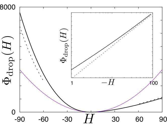
Figure 1: The rate function $\Phi_{\text{drop}}(H)$ (solid black line) which describes the distribution (4) of the KPZ height $H=H(t)$ at small time obtained in (22). The dashed black lines correspond respectively to the left and right tails given in (5), (7) and the purple line corresponds to the Edward-Wilkinson Gaussian regime (6). Inset: Log-log plot of the left tail compared with the asymptotics (5).

It is then natural to wonder: are these tails $P(H,t)\sim e^{-|H|^{3}/(12t)}$ ($H$ large negative) and $\sim e^{-\frac{4}{3}H^{3/2}/t^{1/2}}$ ($H$ large positive) visible only at late times, or do they appear even at early times? It is well known that the central typical regime at early times is described by a Gaussian – obtained from the Edwards-Wilkinson’s (EW) equation EW setting $\lambda_{0}=0$ in the KPZ equation. What about the tails? Recently, Meerson et al. Baruch studied this question for the flat initial condition using the weak noise theory (WNT) (see also earlier results Korshunov ), valid for short times. For the right tail they found $\sim e^{-\frac{4}{3}H^{3/2}/t^{1/2}}$, i.e. the same leading order result as late times. This shows that the asymptotic right tail is established even at early times. In contrast, for the left tail they found $P(H,t)\sim e^{-\frac{8}{15\pi}|H|^{5/2}/t^{1/2}}$ at early times (in our units). This $|H|^{5/2}$ tail behavior for large negative $H$ for flat initial condition is manifestly different from the $|H|^{3}$ tail behavior at late times for the droplet initial condition. This raises the question whether this difference is due to the change in initial conditions, or whether early and late time left tails are different for any given initial condition.

In this Letter, we show that the early time PDF $P(H,t)$ for the droplet initial condition takes the form

$$P(H,t)\sim\exp\left(-\frac{\Phi_{{\rm drop}}(H)}{\sqrt{t}}\right),\quad H~{}\text{fixed}~{}\text{and}~{}t\ll 1$$ (4)

where $\Phi_{{\rm drop}}(H)$ is given explicitly by Eq. (22) below. The asymptotic behaviors of $\Phi_{{\rm drop}}(H)$ are obtained as

$$\Phi_{\rm drop}(H)\simeq \frac{4}{15\pi}|H|^{5/2}\quad,\quad H\to-\infty$$ (5)

$$\Phi_{\rm drop}(H)\simeq \frac{H^{2}}{\sqrt{2\pi}}\quad,\quad|H|\ll 1$$ (6)

$$\Phi_{\rm drop}(H)\simeq \frac{4}{3}H^{3/2}\quad,\quad H\to+\infty\;.$$ (7)

The first three cumulants of $H$ obtained from Eqs. (4) and (22) are in agreement with the leading small time behavior obtained in CLR10 , while here we obtain all cumulants. In the case of the flat initial condition one expects a similar form Baruch , $P(H,t)\sim e^{-\frac{\Phi_{{\rm flat}}(H)}{\sqrt{t}}}$. However, the function $\Phi_{{\rm flat}}(H)$ has not been obtained explicitly apart from the tails footnote1 ; footnoteGaussian and the first two cumulants Baruch ; flatshorttime . Therefore the $|H|^{5/2}$ left tail seems to hold for a variety of initial conditions. Interestingly, as discussed below, our main results, Eqs. (4) and (22), turn out to be very reminiscent of the universal large deviation fluctuations obtained in the stationary regime of finite-size models in the KPZ universality class DerridaLebowitz ; DerridaAppert ; bb-00 ; Povo ; LeeShortTime ; CurrentASEP ; Prolhac_PhD .

Remarkably, these results for the 1D classical KPZ equation can be applied to an apriori different quantum problem of $N$ non-interacting fermions in a one-dimensional harmonic trap, using a recent mapping between the two problems FermionsUS . Under this mapping, the time $t$ in the KPZ equation corresponds to $N/T^{3}$ where $T$ is the (dimensionless) temperature of the fermionic system. In particular it was shown FermionsUS that the fluctuations of the (dimensionless) position of the rightmost fermion ${\sf x}_{\rm max}$ near the edge ${\sf x}_{{\rm edge}}$ of the Fermi gas, are related to those of the KPZ height at the origin $h(0,t)$, as

$$\frac{{\sf x}_{{\rm max}}-{\sf x}_{{\rm edge}}}{w_{N}}\equiv_{\rm in\,law}\frac{h(0,t)+\frac{t}{12}+\gamma}{t^{1/3}}$$ (8)

where $\equiv_{\rm in\,law}$ means identical PDF’s. Here, on the l.h.s. $N$ is large, ${\sf x}_{{\rm edge}}=\sqrt{2N}$ and $w_{N}=N^{-1/6}/\sqrt{2}$. On the r.h.s. $\gamma$ is a Gumbel distributed random variable with PDF given by $P(\gamma)=e^{-\gamma-e^{-\gamma}}$, independent of the height $h(0,t)$. This equivalence in law is valid in the limit of $N\to+\infty$, $T\to+\infty$ but with the ratio $t=N/T^{3}$ fixed. Therefore our short time results for the KPZ equation, lead to exact predictions (29) for the high temperature behavior of the rightmost fermion.

Here for definiteness we focus on the narrow wedge initial condition, $h(x,0)=-|x|/\delta-\ln(2\delta)$, with $\delta\ll 1$. This initial condition gives rise to a curved (or droplet) mean profile as time evolves  SS10 ; CLR10 ; DOT10 ; ACQ11 ; reviewCorwin . We focus on the shifted height at a given space point, and define footnote2

$$H(t)=h(x,t)+\frac{x^{2}}{4t}+\frac{t}{12}+\frac{1}{2}\ln(4\pi t)\;.$$ (9)

The starting point of our calculation is the exact formula for the following generating function, obtained in  SS10 ; CLR10 ; DOT10 ; ACQ11

$$\bigg{\langle}\exp\left(-\frac{e^{H(t)-st^{1/3}}}{\sqrt{4\pi t}}\right)\bigg{\rangle}=Q_{t}(s)$$ (10)

$$Q_{t}(s):={\rm Det}[I-P_{0}K_{t,s}P_{0}]$$ (11)

where $\langle\ldots\rangle$ denotes an average over the KPZ noise. Here $Q_{t}(s)$ is a Fredholm determinant associated to the kernel

$$K_{t,s}(r,r^{\prime}):=\int_{-\infty}^{+\infty}du\,Ai(r+u)Ai(r^{\prime}+u)\sigma_{t,s}(u)$$ (12)

defined in terms of the Airy function $Ai(x)$ and the weight functions

$$\sigma_{t,s}(u):=\sigma(t^{1/3}(u-s))\quad,\quad\sigma(v):=\frac{1}{1+e^{-v}}\;.$$ (13)

In (11), $P_{0}$ denotes the projector on the interval $r\in[0,+\infty[$. In principle, the formula (10) allows us to obtain, via a Laplace inversion, the PDF of $H(t)$ for arbitrary $t$. The resulting expression SS10 ; CLR10 ; ACQ11 is quite complicated: it has been analyzed at large time, but is not very convenient for a finite time analysis. We now show how to extract the small time behavior directly from the generating function (10).

It is convenient to introduce the kernel

$$\bar{K}_{t,s}(u,u^{\prime})=K_{\rm Ai}(u,u^{\prime})\sigma_{t,s}(u^{\prime})$$ (14)

defined in terms of the Airy kernel

$$K_{\rm Ai}(u,u^{\prime})=\int_{0}^{+\infty}drAi(r+u)Ai(r+u^{\prime})$$ (15)

From (14) and (15), one checks that ${\rm Tr}\,\bar{K}_{t,s}^{p}={\rm Tr}(P_{0}K_{t,s}P_{0})^{p}$ for any integer $p\geq 1$, which allows us to rewrite footnote_Fredholm

$$\!\ln{\rm Det}[I-P_{0}K_{t,s}P_{0}]=\ln{\rm Det}[I-\bar{K}_{t,s}]=\sum_{p=1}^{+\infty}\frac{-1}{p}{\rm Tr}\,\bar{K}_{t,s}^{p}$$ (16)

a convenient form to study the small $t$ limit.

We now illustrate the small time analysis on the first term $p=1$ of this series, the general term being analyzed in SuppMat . One has

$${\rm Tr}\,\bar{K}_{t,s}=\int_{-\infty}^{+\infty}duK_{\rm Ai}(u,u)\sigma(t^{1/3}(u-s))$$

$$=t^{-1/3}\int_{-\infty}^{+\infty}dvK_{\rm Ai}\left(\frac{v}{t^{1/3}},\frac{v}{t^{1/3}}\right)\sigma(v-\tilde{s})$$ (17)

where we have performed the change of variable $u=v/t^{1/3}$ and defined $\tilde{s}=st^{1/3}$. We see on this equation that the small $t$ limit is controled by the large argument behavior of the Airy kernel. Since it is decreasing exponentially fast at positive large arguments, we only need its behavior for large negative arguments. To treat arbitrary $p$ in the equation (16) we need the following asymptotic estimate, valid for $v<0$ and $w$ fixed (see SuppMat )

$$K_{\rm Ai}\left(\frac{v}{t^{1/3}},\frac{v+t^{1/2}w}{t^{1/3}}\right)\simeq_{t\ll 1}\frac{1}{\pi t^{1/6}}\frac{\sin\sqrt{|v|}w}{w}\,.$$ (18)

We can thus replace $K_{\rm Ai}(\frac{v}{t^{1/3}},\frac{v}{t^{1/3}})$ by $\frac{\sqrt{|v|}}{\pi t^{1/6}}\theta(-v)$ in (17). This leads to leading order for small $t$

$${\rm Tr}\,\bar{K}_{t,s}\simeq\frac{1}{\sqrt{t}}I_{1}(\tilde{s})\;,$$ (19)

where we defined $I_{p}(\tilde{s}):=\frac{1}{\pi}\int_{-\infty}^{0}dv\sqrt{|v|}\left(\sigma(v-\tilde{s})\right)^{p}$. Remarkably, this small $t$ estimate (19) can be generalized to all $p$ to obtain the leading behavior ${\rm Tr}\,\bar{K}_{t,s}^{p}\simeq I_{p}(\tilde{s})/\sqrt{t}$ SuppMat . The series (16) can then be summed up, leading to

$$\ln Q_{t}(s)\simeq-\frac{1}{\sqrt{t}}\Psi(e^{-\tilde{s}})\;,\;\Psi(z)=-\frac{1}{\sqrt{4\pi}}Li_{\frac{5}{2}}(-z)$$ (20)

in terms of the poly-logarithm function $Li_{\nu}(x)=\sum_{p=1}^{+\infty}{x^{p}}/{p^{\nu}}$.

Hence the exact formula for the generating function (10) takes the following form at small time

$$\bigg{\langle}\exp\left(-\frac{z}{\sqrt{4\pi t}}e^{H(t)}\right)\bigg{\rangle}\sim e^{-\frac{1}{\sqrt{t}}\Psi(z)}$$ (21)

where we use $z=e^{-\tilde{s}}$. Note that the l.h.s. is finite only for $z>0$ (for $z<0$ it is infinite).

From this, assuming the form (4) and inserting it in (21) for any $z>0$, we obtain $\Phi_{\rm drop}(H)$ by a saddle point analysis SuppMat , as

$$\!\!\Phi_{\rm drop}(H)=\begin{cases}\frac{-1}{\sqrt{4\pi}}\displaystyle\min_{\begin{subarray}{c}z\in[-1,+\infty[\end{subarray}}[ze^{H}+Li_{\frac{5}{2}}(-z)],\;H\leq H_{c}\\ \\ \frac{-1}{\sqrt{4\pi}}\displaystyle\min_{z\in[-1,0[}[ze^{H}+Li_{\frac{5}{2}}(-z)\\ ~{}~{}~{}~{}~{}~{}~{}~{}~{}~{}~{}~{}~{}~{}~{}-\frac{8\sqrt{\pi}}{3}(-\ln(-z))^{\frac{3}{2}}],\;H\geq H_{c}\end{cases}$$ (22)

where $H_{c}=\ln\zeta(3/2)=0.96026..$. Note that despite the two apparent branches, the function $\Phi_{\rm drop}(H)$ is analytic at $H=H_{c}$. From this expression one obtains the asymptotic behaviors given in Eqs. (5-7) SuppMat . One can also compute the cumulants of the height as, $\overline{H(t)^{q}}^{c}=t^{\frac{q-1}{2}}\phi^{(q)}(0)$, where $\phi^{(q)}$ is the $q$-th derivative of

$$\phi(p)=\max_{H}(pH-\Phi_{\rm drop}(H))\,.$$ (23)

We display here the first four cumulants

$$\overline{H^{2}}^{c}=\sqrt{\frac{\pi}{2}}t^{1/2}\quad,\quad\overline{H^{3}}^{c}=(\frac{8}{3\sqrt{3}}-\frac{3}{2})\pi t$$ (24)

$$\overline{H^{4}}^{c}=(18+15\sqrt{2}-16\sqrt{6})\frac{\pi^{3/2}}{3}t^{3/2}\;.$$ (25)

Remarkably, these cumulants are very similar to the ones obtained for the stationary fluctuations of the total integrated particle current for the TASEP on a finite ring DerridaLebowitz ; DerridaAppert . This similarity holds for all higher cumulants as well (see SuppMat ). In fact, the generating function associated with these cumulants, called $G$ in DerridaLebowitz ; DerridaAppert also appears in the stationary regime of the ASEP and of the KPZ equation on a finite ring CurrentASEP ; Povo ; bb-00 ; LeeShortTime ; Prolhac_PhD , and is different, but similar to our function $\Psi$. It remains a puzzle why this universal function $G$ describing the late time stationary regime in a finite system should be similar to our short time large deviation function in an infinite system.

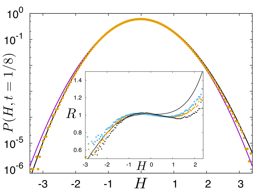
Figure 2: Numerical determination of $P(H,t=1/8)$. In the main figure, the purple line corresponds to the Edward-Wilkinson Gaussian regime (6). The symbols correspond to the numerical data for the discrete model with $\hat{t}=256,\beta=1/16$ (with $2\,.10^{8}$ samples). Note that we have imposed $\langle H\rangle=0$. The black line corresponds to $P(H,t)=c(t)e^{-\Phi_{\text{drop}}(H)/\sqrt{t}}$ (22) where $c(t)=\int_{0}^{\infty}dHe^{-\Phi_{\text{drop}}(H)/\sqrt{t}}$, with $c(1/8)=1.23487\ldots$. Inset: Plot of the ratio $R=P(H,t)/P_{\rm Gauss}(H,t)$ for $t=1/8$, where $P_{\rm Gauss}(H,t)$ corresponds to the Gaussian regime (6). The triangles, circles and squares correspond respectively to $\hat{t}=128$, $\hat{t}=256$ and $\hat{t}=512$. We see that when $\hat{t}$ increases the agreement with the short time continuum limit improves.

Our results also describe the high temperature limit of lattice directed polymer models (DP), which allows for a numerical test. We simulate a DP growing on a 2D square lattice with unit Gaussian site disorder. For inverse temperature $\beta\ll 1$, the number of steps $\hat{t}$ corresponds to the time of the continuum model as $t=2\hat{t}\beta^{4}$ CLR10 (see SuppMat for details). The result for $P(H,t)$ is shown in Fig. 2: the data shows (slow) convergence to our prediction.

Fermions in an harmonic trap. Consider now the quantum problem of $N$ non-interacting spinless fermions of mass $m$ in an harmonic trap at finite temperature $T$, described by the Hamiltonian $H=\sum_{i=1}^{N}\frac{p_{i}^{2}}{2m}+\frac{1}{2}m\omega^{2}{x}_{i}^{2}$. We use ${\sf x}^{*}=\sqrt{\hbar/m\omega}$ and $T^{*}=\hbar\omega$ as units of length and energy. At $T=0$, i.e. in the ground state, and for large $N$, the average fermion density is given by the Wigner semi-circle law, with a finite support $[-{\sf x}_{\rm edge},{\sf x}_{\rm edge}]$ where ${\sf x}_{\rm edge}=\sqrt{2N}$. At finite temperature, the behavior of physical quantities in the bulk changes on a temperature scale $T\sim N$ (bulk scaling), while near the edge it varies on a scale $T=N^{1/3}/b$ (edge scaling), where $b$ is a dimensionless parameter of order unity FermionsUS . Here we are interested in the position ${\sf x}_{\rm max}(T)$ of the rightmost fermion (see FermionsUS for a precise definition). Its cumulative distribution function (CDF) was shown FermionsUS to be given by the same Fredholm determinant as in Eq. (11)

$${\rm Prob}\left(\frac{{\sf x}_{max}(T)-{\sf x}_{\rm edge}}{w_{N}}<s\right)=Q_{t=b^{3}}(s)$$ (26)

where $w_{N}=N^{-1/6}/\sqrt{2}$. Since we have already analysed the small time limit $t\ll 1$ of the Fredholm determinant $Q_{t}(s)$ (as in Eq. (20)), this provides us with an explicit formula for the fermion problem, valid in the high temperature region $b\ll 1$ of the edge scaling regime.

To use the result in (20), we first set $s={\tilde{s}}/t^{1/3}$ in (26) where $t^{1/3}=N^{1/3}/T$. The regime $t\ll 1$ corresponds to $T\gg N^{1/3}$. This leads us to define a new random variable

$$\xi=\frac{{\sf x}_{\max}(T)-{\sf x}_{\rm edge}}{w_{N}(T)}$$ (27)

with

$$w_{N}(T):=TN^{-1/3}w_{N}=T/\sqrt{2N}$$ (28)

where $w_{N}=N^{-1/6}/\sqrt{2}$ is the scale of fluctuations of ${\sf x}_{\rm max}$ at $T=0$. Thus $w_{N}(T)$ in (28) sets the scale of fluctuations of ${\sf x}_{\rm max}$ for $T\gg N^{1/3}$. Using (20) in the limit $t=b^{3}=N/T^{3}\ll 1$, we find that the CDF of $\xi$ takes the asymptotic form (replacing $\tilde{s}$ by $s$ for convenience)

$${\rm Prob}(\xi<s)\sim\exp\left(\sqrt{\frac{T^{3}}{4\pi N}}Li_{5/2}(-e^{-s})\right)\,.$$ (29)

Using $Li_{5/2}(y)\simeq y$ for small $y$, it is easy to see that the PDF of $\xi$ is peaked around the typical value $\xi=\xi_{\rm typ}=\frac{1}{2}\ln(T^{3}/4\pi N)$, with typical fluctuations $\tilde{\xi}=\xi-\xi_{\rm typ}$ described by a Gumbel law, i.e., $P(\tilde{\xi})=e^{-\tilde{\xi}-e^{-\tilde{\xi}}}$ (see Joh07 for a similar observation in a related model).

Our formula (29), however, holds beyond the typical fluctuation regime and also describes the large deviations away from $\xi_{\rm typ}$. While the right tail is exponential, as given by the Gumbel distribution, using $Li_{\frac{5}{2}}(-z)\simeq_{z\to+\infty}-\frac{8}{15\sqrt{\pi}}(\ln z)^{\frac{5}{2}}$ in (29), we find that the left tail exhibits a distinct, stretched exponential decay

$${\rm Prob}(\xi<s)\sim\exp\left(-\frac{4}{15\pi}\sqrt{\frac{T^{3}}{N}}|s|^{5/2}\right)\,.$$ (30)

Note that in this edge regime quantum correlations are still important. At much higher temperatures $T\sim N$, the positions of the fermions become completely independent variables, and the fluctuation of ${\sf x}_{\rm max}(T)$ is also described by a Gumbel distribution, albeit different from the one obtained here longUS .

The above method is easily extended to obtain the full counting statistics (FCS) of the fermions near the edge for temperatures $T\gg N^{1/3}$. This is a generalisation of the $T=0$ result for the FCS in the edge regime Eisler2013 . Denoting by $N(s)$ the number of fermions in the interval $[{\sf x}_{\rm edge}+s\,w_{N}(T),+\infty[$ we obtain the characteristic function (see (49) in SuppMat ) and, from it, the cumulants

$$\langle\big{(}N(s)\big{)}^{p}\rangle^{c}\simeq-\sqrt{\frac{T^{3}}{4\pi N}}\,Li_{\frac{5}{2}-p}(-e^{-s})$$ (31)

for all positive integer $p\geq 1$. In the typical region defined above, $s-\xi_{\rm typ}={\cal O}(1)$ the statistics is Poisson with mean $\langle N(s)\rangle\simeq e^{\xi_{\rm typ}-s}$. There are deviations from Poisson in the tails, in particular for $s-\xi_{\rm typ}\to-\infty$ where the distribution becomes peaked around $\langle N(s)\rangle\simeq\sqrt{\frac{T^{3}}{4\pi N}}\frac{4(-s)^{3/2}}{3\sqrt{\pi}}$ with $\langle N(s)^{2}\rangle^{c}\simeq\sqrt{\frac{T^{3}}{4\pi N}}\frac{2\sqrt{-s}}{\sqrt{\pi}}$ and zero higher cumulants.

In conclusion we have studied the statistics of the height fluctuations for the continuum KPZ equation at short time with the droplet initial condition. We obtained the exact analytical rate function $\Phi_{\rm drop}(H)$ and compared with numerics. It confirms, and extends, through an exact solution, recent approaches using weak noise theory developed for the flat geometry and unveils puzzling similarities with other large deviation results for finite-size system. We demonstrate that, remarkably, the right tail coincides with the Tracy-Widom result already at short time. This result agrees with rigorous bounds Chen valid at any fixed time $t$, $P(H>s)\leq e^{-\frac{4}{3}s^{3/2}/t^{1/2}}$. By contrast the convergence towards the left TW tail $\sim(-H)^{3}$ appears to be much slower, with $\sim(-H)^{5/2}$ behavior at short time. Our short-time results for the KPZ equation also provide exact asymptotic predictions for the PDF of the rightmost fermion in a harmonic trap at high temperature $T\gg N^{1/3}$. We hope that the present results will stimulate further investigations of extreme value questions in the KPZ class Khoshnevisan and also in cold atom systems.

We thank D. S. Dean, K. Johansson, D. Khosnevisan, B. Meerson, J. Quastel, T. Sadhu, H. Spohn and K. Takeuchi for useful discussions. We acknowledge support from PSL grant ANR-10-IDEX-0001-02-PSL (PLD). We thank the hospitality of KITP, under Grant No. NSF PHY11-25915.

.

SUPPLEMENTARY MATERIAL

We give the principal details of the calculations described in the manuscript of the Letter.

I 1. Short time estimate of the Fredholm determinant $Q_{t}(s)$

We start by deriving the formula for $Q_{t}(s)$ given in Eq. (20) in the Letter. From Eqs. (11) and (16) given in the Letter, one has

$$\ln Q_{t}(s)=-\sum_{p=1}^{\infty}\frac{1}{p}{\rm Tr}\,\bar{K}^{p}_{t,s}\;,\;\bar{K}_{t,s}(u,u^{\prime})=K_{\rm Ai}(u,u^{\prime})\sigma_{t,s}(u^{\prime})$$ (32)

where $K_{\rm Ai}(u,u^{\prime})$, the Airy kernel, and $\sigma_{t,s}$ are given in Eqs. (15) and (13) of the Letter (respectively). Hence one has

$${\rm Tr}\;{\bar{K}}_{t,s}^{p}=\int_{-\infty}^{\infty}dv_{1}\int_{-\infty}^{\infty}dv_{2}\ldots\int_{-\infty}^{\infty}dv_{p}K_{\rm Ai}(v_{1},v_{2})..K_{\rm Ai}(v_{p},v_{1})\sigma_{t,s}(v_{1})\ldots\sigma_{t,s}(v_{p})$$ (33)

The expression of $\sigma_{t,s}(v)=\sigma(t^{1/3}(v-s))$ suggests to perform the change of variable $v_{i}\to v_{i}/t^{1/3}$, which yields (setting $\tilde{s}=st^{1/3}$):

$${\rm Tr}\;{\bar{K}}_{t,s}^{p} = t^{-p/3}\int_{-\infty}^{\infty}dv_{1}\int_{-\infty}^{\infty}dv_{2}\ldots\int_{-\infty}^{\infty}dv_{p}\,K_{\rm Ai}\left(\frac{v_{1}}{t^{1/3}},\frac{v_{2}}{t^{1/3}}\right)\ldots K_{\rm Ai}\left(\frac{v_{p}}{t^{1/3}},\frac{v_{1}}{t^{1/3}}\right)\sigma(v_{1}-\tilde{s})\ldots\sigma(v_{p}-\tilde{s})$$ (34)

$$\sigma(v) = \frac{1}{e^{-v}+1}\;.$$

Let us now recall the two useful representations of the Airy kernel

$$K_{\rm Ai}(u,u^{\prime})=\int_{0}^{+\infty}drAi(r+u)Ai(r+u^{\prime})=\frac{Ai(u)Ai^{\prime}(u^{\prime})-Ai(u^{\prime})Ai^{\prime}(u^{\prime})}{u-u^{\prime}}\;.$$ (35)

From the second expression , and using the asymptotic expansion of the Airy function for the large negative argument ${\rm Ai}(x)\sim\cos{(\pi/4-2|x|^{3/2}/3)}/\sqrt{\pi|x|^{1/2}}$, for $x\to-\infty$, one obtains the limiting form of the Airy kernel as

$$\lim_{t\to 0,v_{1}<0}t^{1/6}K_{\rm Ai}\left(\frac{v_{1}}{t^{1/3}},\frac{v_{1}+t^{1/2}w}{t^{1/3}}\right)=\frac{1}{\pi}\frac{\sin(\sqrt{|v_{1}|}w)}{w}\;.$$ (36)

On the other hand, for $v_{1}>0$, the Airy kernel vanishes exponentially in the limit $t\to 0$ and therefore only the region where all the $v_{i}$ are negative need to be considered in Eq. (34). Hence for $p\geq 2$, separating the center of mass coordinate (which we take as $v_{1}$) and the $p-1$ relative coordinates $v_{j}=v_{j-1}+t^{1/2}w_{j}$ we obtain

$${\rm Tr}\bar{K}^{p}\simeq t^{-p/3}\int_{-\infty}^{0}dv_{1}\left(\frac{1}{\pi t^{1/6}}\right)^{p}[\sigma(v_{1}-\tilde{s})]^{p}t^{(p-1)/2}$$ (37)

$$\times\int_{-\infty}^{\infty}dw_{1}\ldots\int_{-\infty}^{\infty}dw_{p}\frac{\sin(\sqrt{|v_{1}|}w_{1})}{w_{1}}\frac{\sin(\sqrt{|v_{1}|}w_{2})}{w_{2}}\ldots\frac{\sin(\sqrt{|v_{1}|}w_{p})}{w_{p}}\delta(w_{1}+w_{2}+..+w_{p})$$

$$=\frac{1}{\pi^{p}\sqrt{t}}\int_{-\infty}^{0}dv_{1}\sqrt{|v_{1}|}[\sigma(v_{1}-\tilde{s})]^{p}I_{p}\;,\;I_{p}=\int_{-\infty}^{\infty}dw_{1}\ldots\int_{-\infty}^{\infty}dw_{p}\frac{\sin w_{1}}{w_{1}}\frac{\sin w_{2}}{w_{2}}..\frac{\sin w_{p}}{w_{p}}\delta(w_{1}+..+w_{p})\;.$$ (38)

The multiple integral defining $I_{p}$ in Eq. (38) can be computed explicitly, using $\sin{x}/x=(1/2)\int_{-1}^{1}e^{ikx}dk$ and an integral representation of the delta function in Eq. (38), to obtain

$$I_{p}=\frac{1}{2^{p}}\int_{-1}^{1}dx_{1}\ldots\int_{-1}^{1}dx_{p}\int_{-\infty}^{\infty}\frac{dk}{2\pi}\int_{-\infty}^{\infty}dw_{1}\ldots\int_{-\infty}^{\infty}dw_{p}e^{i\sum_{j=1}^{p}(x_{j}+k)w_{j}}=\frac{1}{2^{p}}(2\pi)^{p}\int_{-1}^{1}\frac{dk}{2\pi}=\pi^{p-1}\;.$$ (39)

Thus, from Eq. (32) together with Eqs. (38) and (39), one obtains

$$\ln Q_{t}(s)\approx-\frac{1}{\sqrt{t}}\Psi(e^{-\tilde{s}})$$ (40)

$$\Psi(z)=\frac{1}{\pi}\sum_{p=1}^{\infty}\frac{1}{p}\int_{-\infty}^{0}dv\sqrt{|v|}\frac{1}{(e^{-v}z^{-1}+1)^{p}}=\frac{1}{\pi}\sum_{p=1}^{\infty}\frac{1}{p}\int_{0}^{+\infty}dv\sqrt{v}\left(\frac{ze^{-v}}{(1+ze^{-v})}\right)^{p}$$ (41)

It is then straightforward to perform the sum over $p$ to get

$$\Psi(z) = -\frac{1}{\pi}\int_{0}^{+\infty}dv\sqrt{v}\ln\left(1-\frac{ze^{-v}}{1+ze^{-v}}\right)=\frac{1}{\pi}\int_{0}^{+\infty}dv\sqrt{v}\ln(1+ze^{-v})$$ (42)

$$= -\frac{1}{\sqrt{4\pi}}Li_{5/2}(-z)\;,$$ (43)

as given in the Letter in Eq. (20).

II 2. Counting statistics from a generalized Fredholm determinant

We give here the details of the calculation of the characteristic function for the full counting statistics, and from it the cumulants of the fermion number (31) displayed in the text, since it is a very simple modification of the previous calculation. We use the fact that the quantum probability measure on the fermion positions $x_{i}$ becomes a determinantal process in the limit of large $N$ FermionsUS_app .

Denoting as in the text, $N(s)$, the total number of fermions in the interval $[s,+\infty[$ we can use the standard property of a determinantal process to express the Laplace transform of its distribution as

$$\langle e^{-\lambda N(s)}\rangle={\rm Det}[I-(1-e^{-\lambda})P_{0}K_{t,s}P_{0}]={\rm Det}[I-(1-e^{-\lambda})\bar{K}_{t,s}]$$ (44)

where $K_{t,s}$ and $\bar{K}_{t,s}$ are defined respectively in (12) and (14) in the text. So it is a simple generalization of $Q_{t}(s)$, which is recovered for $\lambda=+\infty$. It can thus also be expanded in traces of powers

$$\ln\langle e^{-\lambda N(s)}\rangle=-\sum_{p=1}^{+\infty}\frac{1}{p}(1-e^{-\lambda})^{p}\,{\rm Tr}\,\bar{K}_{t,s}^{p}$$ (45)

Following the same steps as in the previous section, we thus obtain

$$\ln\langle e^{-\lambda N(s)}\rangle\approx-\frac{1}{\sqrt{t}}\Psi(e^{-\tilde{s}},\lambda)$$ (46)

$$\Psi(z,\lambda)=\frac{1}{\pi}\sum_{p=1}^{\infty}\frac{1}{p}\int_{0}^{+\infty}dv\sqrt{v}\left(\frac{z(1-e^{-\lambda})e^{-v}}{(1+ze^{-v})}\right)^{p}=-\frac{1}{\pi}\int_{0}^{+\infty}dv\sqrt{v}\ln\left(1-\frac{z(1-e^{-\lambda})e^{-v}}{1+ze^{-v}}\right)$$ (47)

$$=\frac{1}{\pi}\int_{0}^{+\infty}dv\sqrt{v}(\ln(1+ze^{-v})-\ln(1+ze^{-\lambda}e^{-v}))=-\frac{1}{\sqrt{4\pi}}(Li_{5/2}(-z)-Li_{5/2}(-ze^{-\lambda}))$$ (48)

In the notations of the text, $t\to b^{3}=N/T^{3}$ and $z\to e^{s}$ (note that $\tilde{s}$ is denoted simply $s$ in the part on the fermions) we obtain the characteristic function (as the Laplace transform)

$$\ln\langle e^{-\lambda N(s)}\rangle\simeq\sqrt{\frac{T^{3}}{4\pi N}}[Li_{\frac{5}{2}}(-e^{-s})-Li_{\frac{5}{2}}(-e^{-s-\lambda})]$$ (49)

from which the cumulants (31) given in the text are easily extracted. Note that the fact that in the typical region $s-\xi_{\rm typ}={\cal O}(1)$, the statistics is Poisson can also be seen directly on the above characteristic function since in that limit $\ln\langle e^{-\lambda N(s)}\rangle\simeq-e^{\xi_{\rm typ}-s}(1-e^{-\lambda})$.

III 3. Evaluation of $\Phi_{\rm drop}(H)$

We start from Eq. (21) of the text that reads

$$\left\langle\exp\left(-\frac{z}{\sqrt{4\pi t}}\,e^{H(t)}\right)\right\rangle\sim e^{-\frac{1}{\sqrt{t}}\,\Psi(z)}$$ (50)

where $\Psi(z)=-Li_{5/2}(-z)/\sqrt{4\pi}$ is given in Eq. (25) of the text. Substituting the anticipated form, $P(H,t)\sim e^{-\frac{1}{\sqrt{t}}\,\Phi(H)}$ as $t\to 0$, on the lhs of Eq. (50) gives

$$\left\langle\exp\left(-\frac{z}{\sqrt{4\pi t}}\,e^{H(t)}\right)\right\rangle\sim\int dH\,\exp\left[-\frac{1}{\sqrt{t}}\,\left(\frac{z}{\sqrt{4\pi}}\,e^{H}+\Phi_{\rm drop}(H)\right)\right]\,.$$ (51)

Using $1/\sqrt{t}$ as a large parameter as $t\to 0$, the integral can be evaluated by the saddle point and comparing it to the rhs of Eq. (50) gives

$$\min_{H}\left[\frac{z}{\sqrt{4\pi}}\,e^{H}+\Phi_{\rm drop}(H)\right]=\Psi(z)\,.$$ (52)

Inverting this Legendre transform (assuming convexity of $\Phi(H)$) one gets

$$\Phi_{\rm drop}(H) = \max_{z}\left[-\frac{z}{\sqrt{4\pi}}\,e^{H}+\Psi(z)\right]$$ (53)

$$= -\frac{1}{\sqrt{4\pi}}\min_{z}\left[z\,e^{H}+Li_{5/2}(-z)\right]\,,$$ (54)

where we used $\Psi(z)=-Li_{5/2}(-z)/\sqrt{4\pi}$. Deriving $S_{1}(z)\equiv ze^{H}+Li_{5/2}(-z)$ with respect to $z$ determines the minimizer $z^{*}$, for a given $H$, as

$$e^{H}=-\frac{1}{z^{*}}\,Li_{3/2}(-z^{*})\equiv W_{1}(z^{*})\,,$$ (55)

where we used $\frac{d}{dz}Li_{5/2}(-z)=\frac{1}{z}Li_{3/2}(-z)$. The function $W_{1}(z^{*})$ in Eq. (55) is convergent only in the range $z^{*}\in[-1,\infty]$ and has the following asymptotic properties

$$W_{1}(z^{*}) \simeq -\frac{1}{\Gamma(5/2)}\,\frac{\left(\ln z^{*}\right))^{3/2}}{z^{*}}\quad\,\,{\rm as}\quad z^{*}\to\infty$$ (56)

$$\simeq \zeta(3/2)=2.61238\dots\quad{\rm as}\quad z^{*}\to-1\,.$$ (57)

As one decreases $z^{*}$ from $\infty$ to $-1$, $W_{1}(z^{*})$ thus increases monotonically from $0$ to $\zeta(3/2)=2.61238\dots$ (shown by the solid (black) line in Fig.(3)). Thus, for any given $H\in\left[-\infty,H_{c}=\ln(\zeta(3/2)=0.96026\dots\right]$, there is a unique solution $z^{*}(H)$ of Eq. (55).

Naturally, the question arises: how do we find a solution for $H>H_{c}$? Interestingly, a similar minimization problem also appeared in the compuation of the large deviation function in the asymmetric exclusion problem in a finite ring DL1998 ; DA1999 . The trick is to use the analytically continued partner of $Li_{5/2}(-z)$ (instead of $Li_{5/2}(-z)$) on the rhs of Eq. (54). The correct analytically continued partner DL1998 ; DA1999 of $Li_{5/2}(-z)$ turns out to be, $Li_{5/2}(-z)-\frac{8\sqrt{\pi}}{3}\left[-\ln(-z)\right]^{3/2}$ where $z$ now increases back from $-1$ to $0$. In other words, Eq. (54) is now replaced (for $H>H_{c}$) by

$$\Phi_{\rm drop}(H)=-\frac{1}{\sqrt{4\pi}}\min_{z}\left[z\,e^{H}+Li_{5/2}(-z)-\frac{8\sqrt{\pi}}{3}\,\left[-\ln(-z)\right]^{3/2}\right]\,.$$ (58)

Deriving $S_{2}(z)\equiv z\,e^{H}+Li_{5/2}(-z)-\frac{8\sqrt{\pi}}{3}\,\left[-\ln(-z)\right]^{3/2}$ with respect to $z$ now provides the minimizer $z^{*}$ for $H>H_{c}$

$$e^{H}=-\frac{1}{z^{*}}\,Li_{3/2}(-z^{*})-\frac{4\sqrt{\pi}}{z^{*}}\left[-\ln(-z^{*})\right]^{1/2}\equiv W_{2}(z^{*})\,.$$ (59)

The function $W_{2}(z^{*})$ is defined for all $z^{*}\in[-1,0]$. As $z^{*}$ increases from $-1$ to $0$, the function $W_{2}(z^{*})$ in Eq. (59) increases monotonically (shown by the dashed (red) line in Fig. (3)), with the following limiting behaviors

$$W_{2}(z^{*}) = \zeta(3/2)=2.61238\dots\quad{\rm as}\quad z^{*}\to-1$$ (60)

$$\simeq -\frac{4\sqrt{\pi}}{z^{*}}\left[-\ln(-z^{*})\right]^{1/2}\quad{\rm as}\quad z^{*}\to 0^{-}\,.$$ (61)

Thus, in this range, one can find a unique solution $z^{*}(H)$ of Eq. (59) for any $H\in[H_{c}=\ln(\zeta(3/2)),\infty]$.

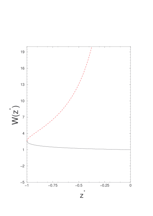
Figure 3: The function $W(z^{*})$ vs $z^{*}$ plotted in the range $z^{*}\in[-1,0]$. The branch $W_{1}(z^{*})$ with $z^{*}\in[-1,\infty]$ is shown by the solid (black) line (plotted only in the regine $z^{*}\in[-1,0]$ for convenience). The branch $W_{2}(z^{*})$ with $z^{*}\in[-1,0]$ is shown by the dashed (red) line. They join smoothly at $z^{*}=-1$ where $W(z^{*})=\zeta(3/2)=2.61238\dots$.

To summarize, for a given $H\in[-\infty,\infty]$, the minimizer $z^{*}$ is determined from the equation

$$e^{H}=W(z^{*})\,$$ (62)

where the function $W(z^{*})$ is given by

$$W(z^{*}) = W_{1}(z^{*})=-\frac{1}{z^{*}}\,Li_{3/2}(-z^{*})\quad{\rm for}\quad z^{*}\in[-1,\infty]\quad{\rm and}\quad H<H_{c}$$ (63)

$$W(z^{*}) = W_{2}(z^{*})=-\frac{1}{z^{*}}\,Li_{3/2}(-z^{*})-\frac{4\sqrt{\pi}}{z^{*}}\left[-\ln(-z^{*})\right]^{1/2}\quad{\rm for}\quad z^{*}\in[-1,0]\quad{\rm and}\quad H>H_{c}\,.$$ (64)

The function $W(z^{*})$ vs $z^{*}$ is plotted in Fig. (3), with the two branches $W_{1}(z^{*})$ (shown by solid (black) line) and $W_{2}(z^{*})$ (shown by the dashed (red) line). We remark that there is no phase transition at $H=H_{c}$, as the function $\Phi(H)$ is analytic at $H=H_{c}$.

IV 4. Asymptotic behavior of $\Phi_{\rm drop}(H)$

Let us derive here the left tail behavior of $\Phi_{\rm drop}(H)$, for $H\to-\infty$. From the saddle point equation (55) we see that it corresponds to $z^{*}\to+\infty$. In that limit we can use the following estimate and $\nu\in\mathbb{N}/2$, $\nu\geq 3/2$ Polylog :

$$Li_{\nu}(-z)\simeq_{z\to+\infty}-\frac{1}{\Gamma(1+\nu)}(\ln z)^{\nu}-\frac{\pi^{2}}{6\Gamma(\nu-1)}(\ln z)^{\nu-2}+..$$ (65)

Hence for $z\to+\infty$ we find that

$$H\simeq-\ln z+\ln(\frac{4}{3\sqrt{\pi}}(\ln z)^{3/2})+..$$ (66)

Inserting back in the formula (54) we finally find

$$\Phi_{\rm drop}(H)\simeq\frac{4}{15\pi}(-H)^{5/2}+\frac{1}{\pi}(-H)^{3/2}\left(\ln(-H)+\frac{2}{3}\left(\ln(\frac{4}{3\sqrt{\pi}})-1\right)\right)+..$$ (67)

which is given in the text.

To obtain the right tail of $\Phi_{\rm drop}(H)$ we write the saddle point equation (59). For large $H$ which corresponds to $z^{*}\to 0$ we can use the asymptotic behavior in (61), i.e. $H\simeq-\ln(-z^{*})+\frac{1}{2}\ln H+\ln(4\sqrt{\pi})$. Reinserting this value of $H$ in (58) evaluated at $z=z^{*}$ we find the two leading orders

$$\Phi_{\rm drop}(H)\simeq_{H\to+\infty}\frac{4}{3}H^{3/2}-(\ln H+2\ln(4\sqrt{\pi})-2)H^{1/2}+..$$ (68)

which is given in the text.

V 5. Short time cumulants of $H$ and relation to Derrida-Lebowitz cumulants

To compute the cumulants of the height $H(t)$ at short times, we first define the cumulant generating function

$$G(p,t)=\left\langle e^{\frac{p}{\sqrt{t}}\,H}\right\rangle=\int e^{\frac{p}{\sqrt{t}}\,H}\,P(H,t)\,dH\,,$$ (69)

where $P(H,t)$ is the height pdf. Substituting the short time form, $P(H,t)\sim e^{-\frac{1}{\sqrt{t}}\,\Phi_{\rm drop}(H)}$ in Eq. (69) and performing the integral by the saddle point method as $t\to 0$ gives

$$G(p,t)\simeq e^{\frac{1}{\sqrt{t}}\,\phi(p)},\quad{\rm where}\quad\phi(p)=\max_{H}\left[pH-\Phi_{\rm drop}(H)\right]\,,$$ (70)

where $\Phi_{\rm drop}(H)$ is given explicitly in Eq. (27) of the text. We note that, be definition, the logarithm of $G(p,t)$ generates the height cumulants by the

$$\ln G(p,t)=\sum_{q=1}^{\infty}\overline{H(t)^{q}}^{c}\,\left[\frac{p}{\sqrt{t}}\right]^{q}\,.$$ (71)

Hence, taking logarithm on both sides of Eq. (70), using (cum1.3) and matching powers of $p$ gives

$$\overline{H(t)^{q}}^{c}=t^{(q-1)/2}\,\phi^{(q)}(0)\,,$$ (72)

for all $q\geq 1$, where $\phi^{(q)}(0)$ is the $q$-th derivative of $\phi(p)=\max_{H}\left[pH-\Phi_{\rm drop}(H)\right]$ evaluated at $p=0$. Note that the centering of $H$ makes the first cumulant vanish. Using the explicit form of $\Phi_{\rm drop}(H)$ in Eq. (27) of the text, one can obtain $\phi^{(q)}(0)$ explicitly. For example, the first $3$ nonzero cumulants are given by

$$\phi^{(2)}(0) = \sqrt{\frac{\pi}{2}}$$ (73)

$$\phi^{(3)}(0) = \left(\frac{8}{3\sqrt{3}}-\frac{3}{2}\right)\pi$$ (74)

$$\phi^{(4)}(0) = \frac{1}{3}\,\left(18+15\sqrt{2}-16\sqrt{6}\right)\pi^{3/2}\,$$ (75)

$$\phi^{(5)}(0) = 120\,\left(-\frac{317}{432}-\frac{1}{\sqrt{2}}+\frac{2}{\sqrt{3}}+\frac{16}{25\sqrt{5}}\right)\pi^{2}$$ (76)

Remarkably, these cumulants carry an uncanny resemblance to the late time cumulants of the total integrated current in the totally asymmetric exclusion process (TASEP) on a ring of size $N$, derived by Derrida and Lebowitz DL1998 . More precisely, Derrida and Lebowitz considered the TASEP on a finite ring of size $N$ with a fixed density $\rho$ of hard core particles. Each particle attempts a jump to the neighboring site with rate $1$ and succeeds provided the target site is empty. Let $J_{i}(T)$ denote the total current up to time $t$ through the bond $i$, i.e., the total number of particles that have passed through the bond $i$ up to time $T$. They considered the random variable $Y_{T}=\sum_{i=1}^{N}J_{i}(T)$ denoting the total integrated current in the system up to time $T$. Using Bethe ansatz techniques, they were able to compute exactly the cumulants of $Y_{T}$ at late times $T>>N^{3/2}$. The first three nonzero moments are given by DL1998

$$\overline{Y_{T}^{2}}^{c} = T\,N^{3/2}\,\left[\rho(1-\rho)\right]^{3/2}\,\frac{\sqrt{\pi}}{2}$$ (77)

$$\overline{Y_{T}^{3}}^{c} = T\,N^{3}\,\left[\rho(1-\rho)\right]^{2}\,\left(\frac{3}{2}-\frac{8}{3\sqrt{3}}\right)\,\pi$$ (78)

$$\overline{Y_{T}^{4}}^{c} = T\,N^{9/2}\,\left[\rho(1-\rho)\right]^{5/2}\,(18+15\sqrt{2}-16\sqrt{6})\frac{\pi^{3/2}}{2\sqrt{2}}$$ (79)

$$\overline{Y_{T}^{5}}^{c} = T\,N^{6}\,\left[\rho(1-\rho)\right]^{3}\,120\,\left(-\frac{317}{432}-\frac{1}{\sqrt{2}}+\frac{2}{\sqrt{3}}+\frac{16}{25\sqrt{5}}\right)\pi^{2}\,.$$ (80)

Naively, the numerical factors on the rhs of Eq. (80), do not look similar to the numerical factors on the rhs of Eq. (76). Remarkably, when slightly re-arranged, they however look very similar! To see this more clearly, we define the ratio

$$R_{q}^{c}=\frac{\overline{Y_{T}^{q}}^{c}}{\overline{H(t)_{t}^{q}}^{c}}\,.$$ (81)

From Eqs. (76) and (80), one finds that the ratio is rather simple and for general $2\leq q\leq 5$, it reads

$$R_{q}^{c}=(-1)^{q}(q-1)\,\,\frac{T}{(2t)^{(q-1)/2}}\,N^{3(q-1)/2}\,\left[\rho(1-\rho)\right]^{(q+1)/2}\,,$$ (82)

with all the strange looking numerical factors disappearing totally! By computing higher cumulants (not shown here) in the two problems, we have verified that this relation holds also for all integer $q>5$.

We do not quite understand why the numerical factors in the cumulants of these two problems are so simply related. First of all, in the TASEP problem one is considering at a finite size ($N$) system and at late times $T>>N^{3/2}$. Using a mapping between TASEP and a discrete growth model, $Y_{T}$ would translate into the integrated height $Y_{T}\equiv\sum_{i=1}^{N}H_{i}(T)$ where $H_{i}(T)$ denotes the height at site $i$ of the discrete-time growth model DA1999 . Still, the results of Derrida nd Lebowitz hold only at late times $T>>N^{3/2}$. In contrast, in the continuum KPZ equation studied in this paper, we compute the cumulants of the height $H(0,t)$, but at short times $t\to 0$ in an already infinite system. So, even admitting the universality of the KPZ growth equation, there is no apriori reason why these two observables in very different time regimes should have a simple relation between their cumulants. This remains an outstanding puzzle to be understood fully.

VI 6. Directed polymer model and numerical details

To test the validity of our results numerically we simulate a directed polymer (DP) growing on a two dimensional square lattice. We define the partition sum $\tilde{Z}_{i,j}=\sum_{\gamma}e^{-\beta\sum_{(r,s)\in\gamma}V_{r,s}}$ over all paths $\gamma$ directed along the diagonal on a square lattice, with only $(1,0)$ or $(0,1)$ moves, starting in $(0,0)$ and ending in $(i,j)$, where the $V_{r,s}$ are i.i.d. random site variables distributed with a unit centered Gaussian. Introducing “time” $\hat{t}=i+j$ and space $\hat{x}=\frac{i-j}{2}$, $Z_{\hat{x},\hat{t}}=\tilde{Z}_{i,j}$ satisfies:

$$Z_{\hat{x},\hat{t}+1}=(Z_{\hat{x}-\frac{1}{2},\hat{t}}+Z_{\hat{x}+\frac{1}{2},\hat{t}})e^{-\beta V_{\hat{x},\hat{t}+1}}$$ (83)

with $Z_{\hat{x},0}=\delta_{\hat{x},0}$. As discussed in CLR10_app the high temperature limit this DP model maps onto the continuum equation (1) in terms of the variables $x=4\hat{x}\beta^{2}$ and $t=2\hat{t}\beta^{4}$. The corresponding continuum height field (9) at $x=0$ is obtained as $H\equiv\ln Z_{0,\hat{t}}/\langle Z_{0,\hat{t}}\rangle$. The result for $P(H,t)$ is shown in the Fig. 2.

References

(1)
M. Kardar, G. Parisi and Y-C. Zhang, Phys. Rev. Lett. 56, 889 (1986).
(2)
D. A. Huse, C. L. Henley, D. S. Fisher, Phys. Rev. Lett. 55, 2924 (1985);
T. Halpin-Healy, Y-C. Zhang, Phys. Rep. 254, 215 (1995);
J. Krug, Adv. Phys. 46, 139 (1997).
(3)
I. Corwin, Random Matrices: Theory Appl. 1, 1130001 (2012)
(4)
C. A. Tracy, H. Widom, Commun. Math. Phys. 159, 151 (1994);
Commun. Math. Phys. 177, 727 (1996) and
Proceedings of the ICM Beijing, 1, 587 (2002).
(5) K. Johansson, Commun. Math. Phys. 209, 437 (2000).
(6) J. Baik, E. M. Rains J. Stat. Phys. 100, 523 (2000).
(7)
M. Prähofer, H. Spohn, Phys. Rev. Lett. 84, 4882 (2000).
(8) T. Sasamoto, H. Spohn, Phys. Rev. Lett. 104, 230602
(2010).
(9) P. Calabrese, P. Le Doussal, A. Rosso, Europhys. Lett. 90, 20002 (2010).
(10) V. Dotsenko, Europhys. Lett. 90, 20003 (2010).
(11) G. Amir, I. Corwin, J. Quastel, Comm. Pure and Appl. Math.
64, 466 (2011).
(12)
K. A. Takeuchi, M. Sano, Phys. Rev. Lett. 104, 230601 (2010);
K. A. Takeuchi, M. Sano, T. Sasamoto, H. Spohn, Sci. Rep. (Nature) 1, 34 (2011);
K. A. Takeuchi, M. Sano, J. Stat. Phys. 147, 853 (2012).
(13)
L. Miettinen, M. Myllys, J. Merikosks, J. Timonen,
Eur. Phys. J. B 46, 55 (2005).
(14) For a review of recent advances in the KPZ problem, see
T. Halpin-Healy, K. A. Takeuchi,
J. Stat. Phys. 160, 794 (2015).
(15)
P. Le Doussal, S. N. Majumdar, G. Schehr, arXiv:1601.05957.
(16) S. N. Majumdar, G. Schehr,
J. Stat. Mech. P01012 (2014) and references therein.
(17)
F. Colomo, A. G. Pronko, Phys. Rev. E 88 042125 (2013).
(18)
S. F. Edwards and D. R. Wilkinson, Proc. R. Soc. London Ser. A 381, 17 (1982).
(19)
B. Meerson, E. Katzav, A. Vilenkin, Phys. Rev. Lett. 116, 070601 (2016).
(20)
I. V. Kolokolov, S. E. Korshunov,
Phys. Rev. E 80, 031107 (2009);
Phys. Rev. B 78, 024206 (2008);
Phys. Rev. B 75, 140201 (2007).
(21)
Note that in our units where
is given in Baruch .
(22)
Note that the coefficient of the central
Gaussian part depends on the initial condition.
(23)
T. Gueudré, P. Le Doussal, A. Rosso, A. Henry, P. Calabrese, Phys. Rev. E 86, 041151 (2012).
(24)
B. Derrida, J. L. Lebowitz, Phys. Rev. Lett. 80 209 (1998).
(25)
B. Derrida, C. Appert, J. Stat. Phys. 94 1 (1999).
(26)
D. S. Lee, D. Kim, Phys. Rev. E. 59 6476 (1999).
(27)
A. E. Derbyshev, A. M. Povolotsky, V. B. Priezzhev,
Phys. Rev. E. 91, 022125 (2015).
T. C. Dorlas, A. M. Povolotsky, V. B. Priezzhev,
J. Stat. Phys. 135, 483 (2009).
(28)
E. Brunet, B. Derrida, Phys. Rev. E 61, 6789 (2000); Physica A 279, 395 (2000).
(29)
D. S. Lee, D. Kim, J. Stat. Mech. P08014 (2006).
(30)
S. Prolhac, Exact methods for the asymmetric simple exclusion process, PhD thesis, Univ. Paris VI, (2009).
(31)
D. S. Dean, P. Le Doussal, S. N. Majumdar, G. Schehr,
Phys. Rev. Lett. 114, 110402 (2015).
(32)
The continuum solution is related to the physical solution up to a non-universal
shift (i.e. renormalization). Let us call the solution to
a physical KPZ problem with a regularized, i.e.
smooth noise at small scale. Then, above a correspondingly small time and length scale,
the continuum and physical solutions are related as follows
.
It holds for an arbitrary initial condition provided is chosen as the solution of
the free diffusion equation with that initial condition. See flatshorttime
for a more detailed discussion in case of flat initial conditions.
(33)
We recall that, for a trace-class operator such that is well
defined, , where . The effect of the projector
in (11) is simply to restrict the integrals over ’s to the interval .
(34) See supplementary material.
(35)
K. Johansson, Probab. Theory Rel. 138, 75 (2007).
(36)
D. S. Dean, P. Le Doussal, S. N. Majumdar, G. Schehr,
in preparation.
(37) V. Eisler, Phys. Rev. Lett. 111, 080402 (2013).
(38)
More precisely, the result
is proved in: X. Chen,
Ann. I. H. Poincaré B 51 , 1486 (2015) [see formula (1.6) and remark 3.1, using previous works in Bertini ],
and Ann. Probab. to appear, 2015.
It implies the bound in the text, using that
. This bound is believed to be the
exact result Quastel .
(39)
L. Bertini and N. Cancrini,
J. Stat. Phys. 78, 1377 (1995).
(40)
J. Quastel, Private Communication.
(41)
D. Khoshnevisan, K. Kim, Y. Xiao, arXiv:1503.06249
(42)
P. Calabrese, P. Le Doussal,
Phys. Rev. Lett. 106, 250603 (2011);
P. Le Doussal, P. Calabrese, J. Stat. Mech. P0600 (2012).
.

References

(1)
D. S. Dean, P. Le Doussal, S. N. Majumdar, G. Schehr,
Phys. Rev. Lett. 114, 110402 (2015).
(2) B. Derrida and J.L. Lebowitz, Phys. Rev. Lett. 80,
209 (1998).
(3) B. Derrida and C. Appert, J. Stat. Phys. 94, 1
(1999).