Next-to-next-to-leading order QCD analysis of spin-dependent parton distribution functions and their uncertainties: Jacobi polynomials approach
Abstract
We present a first QCD analysis of next-to-next-leading-order (NNLO) contributions of the spin-dependent parton distribution functions (PPDFs) in the nucleon and their uncertainties using the Jacobi polynomial approach. Having the NNLO contributions of the quark-quark and gluon-quark splitting functions in perturbative QCD (Nucl. Phys. B 889 (2014) 351-400), one can obtain the evolution of longitudinally polarized parton densities of hadrons up to NNLO accuracy of QCD. A very large sets of recent and up-to-date experimental data of spin structure functions of the proton , neutron , and deuteron have been used in this analysis. The predictions for the NNLO calculations of the polarized parton distribution functions as well as the proton, neutron and deuteron polarized structure functions are compared with the corresponding results of the NLO approximation. We form a mutually consistent set of polarized PDFs due to the inclusion of the most available experimental data including the recently high-precision measurements from COMPASS16 experiments (Phys. Lett. B 753 (2016) 18-28). We have performed a careful estimation of the uncertainties using the most common and practical method, the Hessian method, for the polarized PDFs originating from the experimental errors. The proton, neutron and deuteron structure functions and also their first moments, , are in good agreement with the experimental data at small and large momentum fraction of . We will discuss how our knowledge of spin-dependence structure functions can improve at small and large value of by the recent COMPASS16 measurements at CERN, the PHENIX and STAR measurements at RHIC, and at the future proposed colliders such as Electron-Ion collider (EIC).
pacs:
13.60.Hb, 12.39.-x, 14.65.BtI Introduction
The "spin crisis" has been a longstanding mystery in high energy particle physics. In 1987, series of experiments proved that the spins of the quarks are only partially responsible for the proton’s overall spin. Thus for a decade, long search for the missing pieces, or contributors, to a proton’s spin have been done. The key question is how the spin of the nucleon is distributed among its constituent partons. That is, the determination and understanding the longitudinal spin structure functions of the nucleon and the behavior of spin-dependent parton distribution functions (PPDFs) appeared as an important issue. Recent years have seen increased theoretical interest and setting up experiments towards the better understanding and precise determinations of the polarized nucleon structure function , specially in HERMES, COMPASS, PHENIX and STAR at a variety of energies.
There are several next-to-leading order (NLO) QCD analysis of the polarized DIS data along with the estimation of their uncertainties in the literature Nocera:2014gqa ; Nocera:2014uea ; Jimenez-Delgado:2014xza ; Jimenez-Delgado:2013boa ; Nocera:2014gqa ; Arbabifar:2013tma ; Monfared:2014nta ; Borah:2014esa ; Khorramian:2010qa ; Blumlein:2010rn ; Leader:2014uua ; Aschenauer:2015ata . These parton sets differ in the choice of experimental data sets, treatment of heavy quarks, details of the QCD analysis such as higher-twist corrections, the form of the polarized PDFs at input scale and the error propagation. In this work we provide, for the first time, a next-to-next-to-leading (NNLO) order QCD analysis of polarized parton distribution functions and their uncertainties using all available and up-to-date deeply inelastic scattering data.
The determination of the longitudinal spin structure of the nucleon has attracted considerable theoretical and experimental interests since the surprising EMC experimental results showed that the quark contributions to the nucleon spin is very small Ashman:1987hv ; Ashman:1989ig . The present knowledge on the longitudinal proton spin structure function, originates from measurements of the asymmetry A in polarized lepton nucleon scattering. In the recent years, the available DIS data which may be used for the determination of polarized PDFs, has been extended impressively. The most up-to-date longitudinal polarized deep inelastic scattering (DIS) experimental data from the COMPASS collaboration Adolph:2015saz ; Alekseev:2007vi ; Alekseev:2009ab ; Adolph:2012vj ; Adolph:2012ca , HERMES collaboration Airapetian:2004zf ; Airapetian:2006vy ; Airapetian:2010ac , PHENIX collaboration Adare:2008qb ; Adare:2008aa ; Adare:2014hsq ; Adare:2010cc ; Adare:2010xa and STAR collaboration Adamczyk:2013yvv ; Adamczyk:2012qj ; Adamczyk:2014ozi ; Aggarwal:2010vc ; Adamczyk:2014xyw provide very precise information to study the spin structure and quark PDFs inside the nucleon. These data include the semi-inclusive particle production, high- jet production, semi inclusive DIS in fixed target experiments and W± boson production in polarized proton-proton collisions.
The purpose of the following paper is to present for the first time a very good quality of the polarized PDFs at NNLO using the analysis of available polarized DIS data, taking into account the most recent data from COMPASS16 measurements Adolph:2015saz . An appealing feature of this QCD analysis of polarized PDFs is that we apply the theoretical predictions at NNLO accuracy in perturbative QCD. A careful estimation of the uncertainties have been performed using the most common Hessian method for the polarized parton distributions of quarks and gluon originating from the experimental errors. It is shown that the present analysis considerably leads to smaller value of uncertainties in comparison with other polarized PDFs in the literature. The Jacobi polynomials approach is used to facilitate the analysis. A detailed comparison with other available polarized PDFs including KATAO Khorramian:2010qa , BB Bluemlein:2002be , GRSV Gluck:2000dy , LSS/LSS06 Leader:2005ci ; Leader:2006xc , DNS deFlorian:2005mw , AAC04/AAC09 Goto:1999by ; Hirai:2008aj , DSSV08/DSSV10 deFlorian:2008mr ; deFlorian:2009vb and the most recent results from AKS14 Arbabifar:2013tma and THK14 Monfared:2014nta have been presented. Due to recent high precision measurements we also revisit our next-to-leading order QCD analysis of longitudinal spin structure of the nucleon and present an updated, more accurate, version of our polarized PDFs at next-to-leading order of QCD. In order to discuss the fit results, we will concentrate on our NNLO fit. Since the outcome for NLO and NNLO polarized PDFs are slightly different, we will show the results of both QCD fits in some figures. We also focus on the roles of the NNLO terms on the polarized PDFs determination by comparing the available NLO results with the present NNLO analysis. Moreover, to establish a meaningful baseline for estimating the impact of higher order corrections and to examine the effect of the change in the NNLO polarized PDFs, we compare our NLO and NNLO analyses which have been extracted from the same DIS data set using exactly the same functional forms for polarized distributions and the same assumptions. The main features of our NNLO parametrization of polarized PDFs are worth emphasizing already at this point. The details of the analysis will be present in the next Sections.
The structure of the present paper is as follows: In Sec. II, we will turn to the method of the polarized structure function analysis based on the Jacobi polynomials approach. In Sec. III, we review the input to the global analysis including the data selection and the input parameterizations of the polarized PDFs and deeply inelastic structure functions. The results of the present polarized PDFs analysis are given in Sec. IV. We will study how much a NNLO determination of spin-dependent structure functions would improve our knowledge of polarized parton distribution functions. In Sec. V, a detailed comparison between the present results and available experimental data are presented. We also have attempted a detailed comparison of our NNLO results with recent results from the literature in this Section. In Sec. VI, we will discuss how our knowledge of spin-dependence structure functions may be improved at small and large value of by the recent COMPASS16 measurements at CERN, PHENIX and STAR measurements at RHIC and at the future proposed colliders such as Electron-Ion collider (EIC). Finally, we have presented our summary and conclusions in Sec. VII.
II Polarized PDFs analysis method
Beyond leading order accuracy of pertuarbative QCD, structure functions are no longer linear combination of quark distributions. At higher order, structure functions are obtained by convoluting the quark and gluon distributions with the corresponding pertuabative coefficient functions. Having the next-to-next-to-leading order (NNLO) contributions of the quark-quark and gluon-quark splitting functions in perturbative QCD Moch:2014sna , one can obtain the evolution of longitudinally polarized parton densities of hadrons up to NNLO order of QCD Cafarella:2005zj . The NNLO spin-dependent proton structure functions, , can be written as a linear combination of polarized parton distribution functions , and as,
where the and are the spin-dependent quark and gluon coefficient functions Lampe:1998eu ; Zijlstra:1993sh The method in which we have employed in the present paper is using the Jacobi polynomials expansion of the polarized structure functions. The detailed of such analysis based on the Jacobi polynomials are presented in our previous works Khorramian:2010qa ; Khorramian:2009xz ; Khorramian:2008yh ; AtashbarTehrani:2007odq and also other groupsBarker:1982rv ; Barker:1983iy ; Krivokhizhin:1987rz ; Krivokhizhin:1990ct ; Chyla:1986eb ; Barker:1980wu ; Kataev:1997nc ; Alekhin:1998df ; Kataev:1999bp ; Kataev:2001kk ; Kataev:2005ci ; Leader:1997kw . In this section we outline a brief review of this method. The Jacobi polynomials expansion method is one of the simplest and fastest algorithm to reconstruct the structure function from the QCD predictions for its Mellin moments. In this method, one can easily expand the polarized structure functions, , in terms of the Jacobi polynomials, , as follows,
| (2) |
where is the order of the expansion terms, is the maximum order of the expansion which normally can be set to 7 and 9. The parameters and are a set of free parameters which normally set to 3 and 0.5, respectively. We have shown in our previous work that by setting the = 7 and 9, = 3, = 0.5, this expansion of the structure function can be achieve to optimal convergence throughout the whole kinematic region constrained by the DIS data. The Q2–dependence of the structure functions are codify in the Jacobi polynomials moments, . The -dependence will be provided by the weight function and the Jacobi polynomials which can be written as,
| (3) |
where the coefficients are combinations of Gamma functions in term of , and . The above Jacobi polynomials have to satisfy the following orthogonality relation,
| (4) |
Consequently one can obtain the Jacobi moments, , using the above orthogonality relations as,
| (5) | |||||
where the Mellin transform introduced as,
| (6) |
Finally the polarized structure function can be written as follows,
| (7) | |||||
This method can also be used to construct the proton and neutron structure functions Khorramian:2009xz ; Khorramian:2008yh .
III Input to the global polarized PDFs fit
III.1 NNLO QCD fits of world data
We have adopted the following standard parameterizations at the input scale of Q = 4 GeV2 for the polarized up-valence , down-valence , sea and gluon distributions,
| (8) |
where the normalization factors, , can be determined as,
| (9) |
Considering SU(3) flavor symmetry, we have . Some latest analysis show that including SIDIS data can help to consider light sea-quark decomposition. In the analysis presented in this paper, we wish to study the impact of inclusive DIS data on the determination of NNLO polarized PDFs based on Jacobi polynomials with flavor symmetric light sea distribution. The impact of SIDIS data on the sea quark distributions will be studied in a separate publication in the near future. The unknown parameters in Eq. 8 will be extracted from fit to experimental data. The normalization factors, , are chosen such that the parameters are the first moments distributions,
| (10) |
For the and polarized valence distributions, the first moment of the corresponding distributions, and , will be obtained as,
| (11) | |||||
| (12) |
The and are the non-singlet combinations of the first moments of the polarized parton distributions corresponding to and . The first moments of the polarized valence quark densities introduced in Eq. 10 can be related to and as measured in neutron and hyperon decays Agashe:2014kda . These constraints lead to the values of and for the and polarized valence distributions, respectively. The Dokshitzer-Gribov-Lipatov-Altarelli-Parisi (DGLAP) evolution equations Dokshitzer:1977sg ; Gribov:1972ri ; Lipatov:1974qm ; Altarelli:1977zs are solved in Mellin space and used in Jacobi polynomial approach. The Mellin transform for the polarized PDFs are defined as,
| (13) | |||||
where is the polarized PDFs as , , and . In the Mellin space, the twist-2 contributions to the polarized structure functions can be written in terms of polarized PDFs, , and , and the corresponding coefficient functions ,
III.2 Data selection, minimization and error calculation
The data in which we used in our NNLO polarized PDFs QCD analysis, are summarized in Table. 1. This table contains the name of the experimental group, the covered kinematic ranges in and , the number of available DIS data points and the fitted normalization shifts . The data used (465 experimental points) cover the following kinematics region: and 1 < Q2 < 96 GeV2. The global fit reported in the present article incorporates: a wide range of the polarized deeply inelastic scattering lepton-nucleon data on spin structure functions Abe:1998wq ; HERM98 ; Adeva:1998vv ; EMCp ; E155p ; HERMpd ; COMP1 ; Adolph:2015saz , Abe:1998wq ; E155d ; Adeva:1998vv ; HERMpd ; COMP2005 ; COMP2006 and E142n ; HERM98 ; E154n ; HERMn ; JLABn2004 ; JLABn2005 . An important and appealing feature of our NNLO QCD analysis of the polarized PDFs is that we used the recently published polarized deeply inelastic scattering data from COMPASS16 Adolph:2015saz . These data sets contain both statistical and systematic errors which added in quadrature. In addition, the normalization errors are generally specified separately.
| Experiment | Ref. | [] | Q2 range (GeV2) | Number of data points | |
| E143(p) | (Abe:1998wq, ) | [0.031-0.749] | 1.27-9.52 | 28 | 0.999402403 |
| HERMES(p) | (HERM98, ) | [0.028-0.66] | 1.01-7.36 | 39 | 1.000386936 |
| SMC(p) | (Adeva:1998vv, ) | [0.005-0.480] | 1.30-58.0 | 12 | 1.000084618 |
| EMC(p) | (EMCp, ) | [0.015-0.466] | 3.50-29.5 | 10 | 1.010741787 |
| E155 | (E155p, ) | [0.015-0.750] | 1.22-34.72 | 24 | 1.024394035 |
| HERMES06(p) | (HERMpd, ) | [0.026-0.731] | 1.12-14.29 | 51 | 0.998865500 |
| COMPASS10(p) | (COMP1, ) | [0.005-0.568] | 1.10-62.10 | 15 | 0.9942871736 |
| COMPASS16(p) | Adolph:2015saz | [0.0035-0.575] | 1.03-96.1 | 54 | 1.0009687352 |
| 233 | |||||
| E143(d) | (Abe:1998wq, ) | [0.031-0.749] | 1.27-9.52 | 28 | 0.9993545553 |
| E155(d) | (E155d, ) | [0.015-0.750] | 1.22-34.79 | 24 | 1.0001291961 |
| SMC(d) | (Adeva:1998vv, ) | [0.005-0.479] | 1.30-54.80 | 12 | 0.9999944683 |
| HERMES06(d) | (HERMpd, ) | []0.026-0.731] | 1.12-14.29 | 51 | 0.9984082065 |
| COMPASS05(d) | (COMP2005, ) | [0.0051-0.4740] | 1.18-47.5 | 12 | 0.9983759396 |
| COMPASS06(d) | (COMP2006, ) | [0.0046-0.566] | 1.10-55.3 | 15 | 0.9997379579 |
| 142 | |||||
| E142(n) | (E142n, ) | [0.035-0.466] | 1.10-5.50 | 8 | 0.9989525725 |
| HERMES(n) | (HERM98, ) | [0.033-0.464] | 1.22-5.25 | 9 | 0.9999732650 |
| E154(n) | (E154n, ) | [0.017-0.564] | 1.20-15.00 | 17 | 1.0003242284 |
| HERMES06(n) | (HERMn, ) | [0.026-0.731] | 1.12-14.29 | 51 | 0.9999512597 |
| Jlab04(n) | (JLABn2004, ) | [0.33-0.60] | 2.71-4.8 | 3 | 0.9997264174 |
| Jlab05(n) | (JLABn2005, ) | [0.19-0.20] | 1.13-1.34 | 2 | 1.0002854347 |
| 90 | |||||
| Total | 465 | ||||
Nominal coverage of the data sets used in our fits for proton, neutron and deuteron are presented in Fig. 1. The plots clearly show that despite remarkable experimental efforts, the kinematical coverage of the present available DIS data being included in analysis of polarized PDFs still rather limited. As we mentioned, the accessed range of momentum fraction is . This coverage can leads to a larger uncertainties for determined polarized PDFs at small . For the gluon distribution, which is the most complicated case for PDF uncertainties and parameterizations, we expected a different treatment at due to the lack of DIS data.
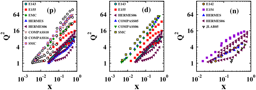
The analysis of value and the error calculation based on the Hessian method are applied in the present analysis. For the error calculation, a standard error analysis is needed for the polarized PDFs by taking into account correlations among the parameters. The resulting eigenvector sets of the determined polarized PDFs can be used to propagate uncertainties to any other desired observable. The method to consider the correlations among the uncertainties is discussed in details in Refs. Khanpour:2016pph ; AtashbarTehrani:2012xh ; Martin:2002aw ; Pumplin:2001ct ; Monfared:2011xf ; Arbabifar:2013tma . Following that, a detailed error analysis has been done using the covariance or Hessian matrix, which can be obtained by running the CERN program library MINUIT James:1994vla .
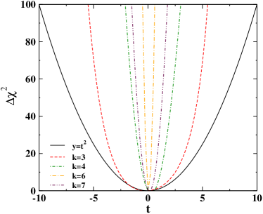
quantifies the goodness of fit to the DIS data for a set of independent parameters that specifies the polarized PDFs at Q = 4 GeV2,
| (15) |
| (16) |
The minimization of the above function is done using the CERN program library MINUIT James:1994vla . In the above equation, , , and denote the experimental measurement, the experimental uncertainty (statistical and systematic combined in quadrature) and the theoretical value for the experimental data point, respectively. is an overall normalization factor for the data of experiment and the is the experimental normalization uncertainty. We allow for a relative normalization shift between different experimental data sets within uncertainties quoted by the experiments. We minimize the above value with the unknown fit parameters plus an undetermined . We find and which yield an acceptable fit to the experimental DIS data. The results show that there is an improvement in the quality of the fit at NNLO.
Some groups such as NNPDF Nocera:2014gqa ; Ball:2013tyh ; Ball:2013lla or JAM Sato:2016tuz propose an alternative approach in their analysis for the PDFs uncertainties, based on an iterative Monte Carlo fitting technique that allows a more robust extraction of polarized PDFs with statistically rigorous PDFs uncertainties. What makes NNPDF differs from others is using neural networks instead of traditional parametrizations. They have presented a global polarized PDFs determination and achieved a significant improvement in accuracy in the determination of the positive polarized gluon distribution in the medium and small- region. In our analysis we utilize, like most of the existing phenomenological spin-dependent PDFs analyses, the standard PDFs fitting technology in which single fits are performed assuming a basic parametric form for the input polarized PDFs. The polarized PDFs errors are then typically computed using the standard error analysis such as Hessian methods proposed by J. Pumplin, D. Stump, Wu-Ki Tung et al. (PST) Pumplin:2001ct ; Martin:2003sk which are based on diagonalization of the matrix of second derivatives for (Hessian matrix) near the minimum of .
| 7.7882 | |||||||||
| 1.535 | 4.97 | ||||||||
| 1.279 | 1.904 | 4.841 | |||||||
| -3.627 | 0.4662 | 9.864 | 0.3169 | ||||||
| 4.861 | -1.075 | 1.923 | 1.454 | 2.479 | |||||
| 2.000 | -4.713 | 1.642 | 8.317 | -1.302 | 0.6388 | ||||
| 2.245 | -5.061 | 3.466 | 0.6800 | -1.568 | -6.909 | 6.700 | |||
| 5.969 | -1.345 | -8.430 | 0.1676 | -4.081 | -1.747 | -1.974 | 8.154 | ||
| -2.137 | -6.011 | 3.375 | 1.1561 | -2.557 | 1.878 | 2.660 | -5.021 | 5.76 |
| 6.806 | |||||||||
| 1.288 | 1.960 | ||||||||
| -3.128 | -4.824 | 8.880 | |||||||
| -6.200 | -2.449 | 5.015 | 1.254E-2 | ||||||
| 7.475 | 2.480 | 3.580 | 5.576 | 3.294 | |||||
| -2.266 | -6.417 | -1.587 | 5.096 | -1.716 | 0.9158 | ||||
| 6.024 | 0.1448 | -1.891 | -0.8584 | 4.692 | -0.1003 | 8.065 | |||
| 2.040 | 5.0283 | -6.372 | -2.602 | 1.471 | -3.088 | 1.685 | 7.072 | ||
| -1.722 | -3.997 | 5.322 | 2.323 | -1.219 | 3.202 | -1.360 | -4.604 | 1.296 |
The Hessian or covariance matrix elements for 9 free parameters of our NNLO and NLO analysis which are obtained by running the CERN program library MINUIT are given in Table 2 and 3. The uncertainties of PDFs can be calculated using these covariance matrix elements based on the Hessian method which can been used as a general statistical method for estimating errors. The uncertainty of polarized PDFs with respect to the optimized parameters is then calculated by using Hessian matrices and assuming linear error propagation,
where the are the elements of the Hessian matrix, is the quantity referring to the parameters which exist in polarized PDFs and indicates the number of parameters which make an extremum value for the related derivative. The polarized PDFs uncertainties at higher scale are calculated by the well-known DGLAP evolution kernel. The Hessian method which is based on the covariance matrix diagonalization, provides an efficient and simple method for calculating the PDFs uncertainties Khanpour:2016pph ; AtashbarTehrani:2012xh ; Pumplin:2001ct ; Martin:2002aw ; Arbabifar:2013tma ; Monfared:2011xf . In this method, one can assume that the deviation in the global goodness-of-fit quantity, , is quadratic in the deviation of the parameters specifying the input parton distributions from their values at the minimum . One can write,
| (18) |
By having a set of appropriate polarized PDFs fit parameters which minimize the global function, , and introducing polarized parton sets , one can write
| (19) |
where is the eigenvalue and is a set of orthonormal eigenvectors. The parameter is adjusted to make the required which is the allowed deterioration in quality for the error determination and is the ideal quadratic behavior. To test the quadratic approximation of Eq. (18), we study the dependence of along some random samples of eigenvector directions. The treatment for some selected eigenvectors, , numbered = 3, 4, 6 and 7 for the presented polarized PDFs analysis are illustrated in Fig. 2. The detailed discussions on error estimation via Hessian method and an investigation of the quadratic behavior of can be found in Refs. Khanpour:2016pph ; AtashbarTehrani:2012xh ; Martin:2002aw ; Monfared:2011xf ; Arbabifar:2013tma ; Pumplin:2001ct . Although technical details are described in mentioned references, we prefer to explain outline of the Hessian method because it is used in our analysis.
The results of our polarized PDFs determination and error estimations will be discussed in much more details in Section. IV.
IV Results of the NNLO polarized PDFs fits
As stated in the Introduction, we intend to study the NNLO polarized PDFs consequently almost all polarized parton distributions in this work are presented in the NNLO order of QCD. In this section we will present and discuss the results of our NNLO QCD analysis to the available world data on polarized inclusive DIS including the up-to-date data from COMPASS16 proton data Adolph:2015saz . Final parameter values for our NNLO and NLO QCD fits and their statistical errors in the –scheme at the input scale = 4 GeV2 are presented in Tables. 4 and 5, respectively. Note that only the experimental errors (including systematic and statistical) are taken into account in this calculations. As seen from the Tables. (4 5), the values of the parameters connected to the polarized PDFs are well determined. The quality of the fit can be judged from the obtained parameters and the values. There is a strong relationship between the input polarized PDFs parameterization and the uncertainties which will be obtained. The parameterization for the input polarized PDFs in our analysis were presented in Section. III, specifically in Eq. 8. The free PDF parameters listed there allow a very large degree of flexibility. The first moments of the polarized valence quark densities introduced in Eq. 10 can be obtain by the constraints presented in Eq. 11 which lead to the values of and for the and polarized valence distributions, respectively.
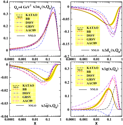
The extracted NNLO polarized PDFs are plotted in Fig. 3 for , , and distributions. The polarized PDFs are compared to those obtained at NLO analysis of KATAO (long dashed) Khorramian:2010qa , BB (dashed) Blumlein:2010rn , DSSV (dashed-dotted) deFlorian:2008mr , GRSV (long dashed-dotted) Gluck:2000dy and AAC09 (dashed-dashed-dotted) Hirai:2008aj . Examining the and polarized valence distributions, we see that most of the fits are in good agreements. However, our result for polarized valance distribution is slightly smaller than others. For the distribution, all of the curve except DSSV are compatible. Let us consider the plot for the polarized gluon distribution; Due to the lack of experimental informations, the prediction for the small- behavior of the polarized gluon distribution , obtained form the different global analyses are largely uncertain. As the plots clearly show, the DSSV result for the gluon distribution has a sign change in the region of , while the other fits are positive. The DSSV family polarized PDFs sets (DSSV deFlorian:2008mr ; deFlorian:2009vb and DSSV+/DSSV++ deFlorian:2011ia ; deFlorian:2014yva ) include some of the non-DIS data of Table 1 such as SIDIS data, inclusive jet and hadron production measurements from polarized proton-proton measurements at RHIC collider. The plots also show that KATAO for the gluon distribution approach to zero more quickly than the other results. The obtained NNLO polarized gluon distribution is slightly smaller as compared to the NLO analysis of BB, GRSV and AAC09, and is positive for wide range of ; .
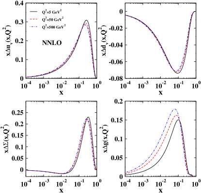
In Fig. 4, we plot the polarized parton distributions as a function of and for different values of Q2 = 5, 50, 500 GeV2. The plot predict an increase of gluon distribution in the kinematic region of by increasing the Q2 values.
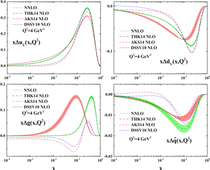
In Fig. 5, we present our polarized parton distributions at Q = 4 GeV2 as a function of in NNLO approximation plotted as a solid curve. Also shown are the most recent results from AKS14 Arbabifar:2013tma , THK14 Monfared:2014nta and the DSSV family polarized PDFs set deFlorian:2009vb . We also illustrate the uncertainties corresponding to the mentioned analysis. Comparing to other results, one finds that the uncertainty band for our NNLO polarized sea distribution for low value of has become slightly narrower than THK14. From the plots, we see that and are reasonably in agreement. The AKS14 and DSSV10 polarized valence distributions slightly approach to zero more quickly than others. For the polarized gluon distribution all of the fits treat differently. The ambiguity in gluon distributions may due to the different theoretical input and also the different data included in the QCD analysis. The AKS14 and DSSV10 polarized gluon distributions have a sign change at . We had this behavior for DSSV08 deFlorian:2008mr polarized gluon distributions presented in Fig. 3. The striking feature of our NNLO polarized gluon distribution is its positivity throughout and clearly away from zero in the regime predominantly probed by the RHIC and COMPASS data. RHIC data mainly probe the region 0.05 0.2, but the recently published data from COMPASS16 Adolph:2015saz which can cover the range of can constrain better down to somewhat lower values of , as we expected form this analysis. Overall, due to lack of enough data for low value of , the constraints on in, say, the regime 0.001 0.05 are still much weaker than those in the region of .
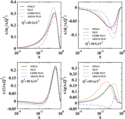
In order to have a detailed comparison, we also plotted the obtained NNLO polarized PDFs as a function of at Q2=10 GeV2 which is presented in Fig. 6. The recent results from AKS14 Arbabifar:2013tma and LSS06 Leader:2006xc analysis also shown. Due to recent high precision measurements we also revisit our next-to-leading order QCD analysis of polarized PDFs. In this plot, we also illustrate our revisited NLO polarized PDFs results which have been extracted using the data presented in Table. 1. The plot shows both of our NLO and NNLO polarized gluon distribution are positive throughout the range.
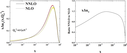
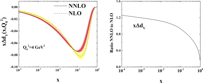
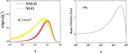
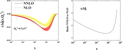
What makes this analysis different from others are using the higher order QCD corrections and the inclusion of more precise data especially the most recent low- data from COMPASS16 experiments. In order to get an idea of the impact of higher order corrections and to examine the effect of the change in the NNLO polarized PDFs, we compare our NLO and NNLO analyses which have been extracted from the same data set using exactly the same functional forms for polarized distributions and the same assumptions. In this respect, we plot the polarized valence distributions in Fig. 7 and polarized sea and gluon distributions in Fig. 8, respectively. The uncertainty bands for NLO and NNLO at 90% C.L. limit which are obtained using the same approach for the input parameterization and error propagation, are also shown as well. In order to illustrate the significance of the size of the differences, we plot the ratios of NNLO polarized PDFs to the corresponding NLO one in the right side of these Figures. The higher order QCD corrections lead to a significant change in the polarized gluon and sea distributions and in the obtained uncertainties. Moreover, there is most improvement in the description of the low- polarized distributions. It is worth mentioning that the uncertainties of the polarized gluon PDFs at low value of still remain large compared to the currently probed region.
In order to examine the effect of PDF parameterisation on the obtained PDF uncertainty, especially for the polarised gluon distribution, we release a few more of the parameters such as the and ,
| (20) |
The result shows that despite of increasing the uncertainties, the shape of the polarized gluon distribution will not changed. In the present work, we only used the usual parametrization for the gluon distribution to have a detailed comparison with the results from THK14 Monfared:2014nta and KATAO Khorramian:2010qa . The difficulties in constraining the polarized gluon distribution are clearly revealed through the spread of from various global PDFs parametrizations illustrated in Figs. 3 and 5. These plot clearly show that depending on the global PDFs parametrizations, the method of PDFs uncertainty estimation and the data sets included in the fits, the shapes and magnitudes from the gluon PDFs including its uncertainty are generally different. In most of the fits the PDFs is positive at large value of with a sign change at smaller value of for THK14 and the DSSV. In both our NLO and NNLO analysis, we obtained a positive PDFs which is clearly away from zero in the regime .
The best-fit values of the first moments of structure function can be obtained using the analyzed polarized PDFs. One can determine the first moment as,
| (21) |
The corresponding results for the first moments using the extracted polarized PDFs are presented in Table. 6 for selected values of Q2.
| Q2 | 2 GeV2 | 5 GeV2 | 10 GeV2 | 50 GeV2 |
|---|---|---|---|---|
| 0.92644 | 0.92589 | 0.92562 | 0.92508 | |
| -0.34116 | -0.34096 | -0.34086 | -0.34066 | |
| 0.285276 | 0.285105 | 0.285019 | 0.28485 | |
| 0.33012 | 0.39138 | 0.426678 | 0.50931 | |
| 0.12187 | 0.13229 | 0.13673 | 0.14393 | |
| -0.05332 | -0.05441 | -0.05492 | -0.05582 | |
| 0.031706 | 0.036019 | 0.037840 | 0.040752 |
The numerical results for the polarized structure functions , and in NNLO approximations are compared with the corresponding data from recently published COMPASS16 results in Table. 7. The table clearly shows our results describe the experimental measurements well.
| COMPASS16 | NNLO (MODEL) | ||
|---|---|---|---|
| 0.139 0.003 0.009 | 0.12742 | ||
| -0.041 0.006 0.011 | -0.05389 | ||
| 0.181 0.008 0.014 | 0.18131 |
| Order | Reference | Notes | |
|---|---|---|---|
| NLO | This analysis | ||
| NLO | Blumlein:2010rn | BB10 | |
| NLO | Khorramian:2010qa | KATAO | |
| NLO | AtashbarTehrani:2007odq | TK | |
| NLO | Owens:2012bv | CJ12 | |
| NLO | Monfared:2014nta | THK14 | |
| NLO | Khanpour:2012tk | KKT12C | |
| NLO | Khanpour:2012tk | KKT12 | |
| NNLO | This analysis | ||
| NNLO | Blumlein:2006be | BBG06 | |
| NNLO | Khorramian:2008yh | KT08 | |
| NNLO | ABKM | ABKM10-FFS | |
| NNLO | ABKM | ABKM10-BSM | |
| NNLO | JR | GRS dynamic approach | |
| NNLO | JR | GRS standard approach | |
| NNLO | MSTW | MSTW08 | |
| NNLO | H1ZEUS | H1 and ZEUS | |
| NNLO | d'Enterria:2015toz | Preliminary | |
| NNNLO | Khorramian:2009xz | KKT10 | |
| NNNLO | Blumlein:2006be | BBG06 | |
| — | Agashe:2014kda | World Average |
In order to check the accuracy of the extracted polarized parton distribution functions, we present the recent results for the running coupling constant in Table. 8. The results obtained by available QCD analysis of inclusive deep-inelastic scattering data in NLO, NNLO and NNNLO approximations including the current world average of Agashe:2014kda are also presented. Our results for the running coupling constant, , also shown as well. We obtained the following value for the strong coupling constant at Z boson mass scale at NNLO approximation,
| (22) |
The higher order QCD correction leads to a larger value of the QCD coupling at NNLO. To close this section, we note that using simple forms of parametrization and enormous amount of constraining data, the NNLO distributions lead to a considerable decrease in the polarized PDFs uncertainties. Detailed comparisons to the various NLO sets and with the data, will be made in the next Section.
V Comparison with the data and different global analyses of polarized PDFs
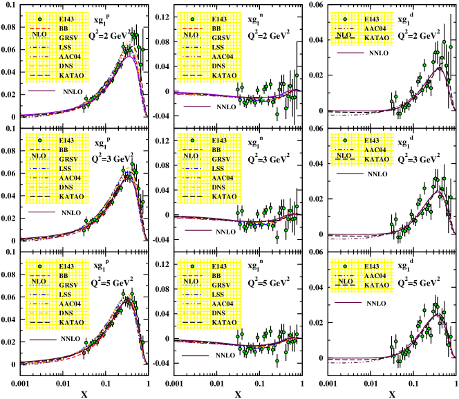
Throughout the above discussion we have presented our NLO and NNLO polarized PDFs including their uncertainties. In the following section, we will present a detailed comparison of our NNLO polarized PDFs with the data and other phenomenological models. In Fig. 9, the spin-dependent structure function of the proton, neutron and deuteron are displayed as a function of at Q2 = 2, 3 and 5 GeV2, respectively. The solid curve represent to our theory predictions for at NNLO approximation. The results of those obtained at NLO from KATAO (long dashed) Khorramian:2010qa , BB (dashed) Bluemlein:2002be , GRSV (dotted) Gluck:2000dy , LSS (dashed-dotted) Leader:2005ci , DNS (dashed-dashed-dotted) deFlorian:2005mw and AAC04 (dashed-dotted-dotted) Goto:1999by also shown as well. Data points are from the E143 Abe:1998wq experiments at SLAC. The good quality of the fits for the best-fit polarized structure functions are apparent from these plots. The poor quality of current knowledge of the shape of polarized parton distributions and structure functions at are a consequence of the limited kinematic coverage of polarized DIS data at small .
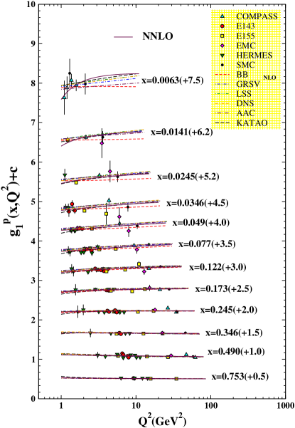
The prediction for the polarized proton structure function as function of Q2 in intervals of is presented in Fig. 10. Our fit is the solid curve in NNLO approximation. The error bars shown are the statistical and systematic uncertainties added in quadrature. The values of the shift parameter are given in parentheses. Also shown are the results of KATAO (long dashed) Khorramian:2010qa , BB (dashed) Bluemlein:2002be , GRSV (dashed-dotted) Gluck:2000dy , LSS (dashed-dotted-dotted) Leader:2005ci , DNS (dashed-dashed-dotted) deFlorian:2005mw and AAC04 (long dashed-dotted) Goto:1999by in NLO approximation.
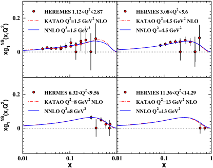
We are in positions to study the behavior of our NNLO polarized parton distributions functions in the regions of small and large momentum fractions. Having investigated the neutron, proton and deuteron spin-dependent structure function, one can turn to the non-singlet spin-dependent structure function as,
| (23) | |||||
where is the nucleon structure function and is the D-state wave probability for the deutron Lacombe:1981eg ; Machleidt:1987hj . The prediction for the non-singlet polarized structure functions as function of in NNLO approximation are plotted in Fig. 11. The NLO result from KATAO Khorramian:2010qa shown for comparison. The plots correspond to the bin , , and , respectively. The plots show that our results for the non-singlet polarized structure functions describe both the data and the results obtained by KATAO analysis well.
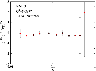
The prediction for the best-fit polarized neutron structure function can also been obtained using analyzed polarized PDFs. In Fig. 12, we plot the ratios of where is the experimental value of the polarized neutron structure function and is the corresponding theoretical values. Also shown are the most recent data from E154 E154n collaborations.
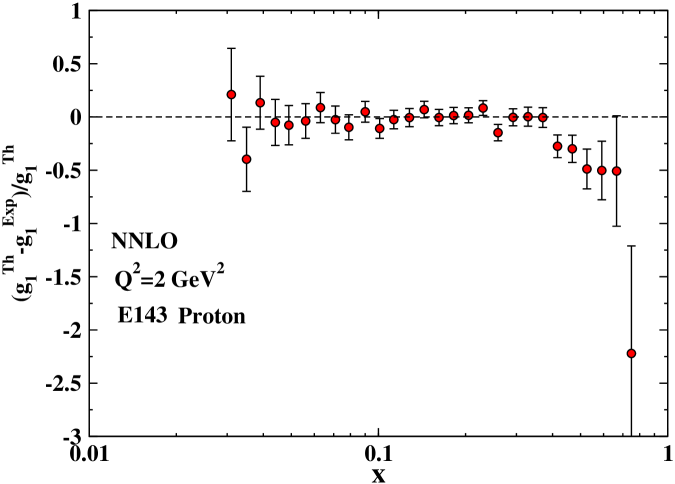
A detailed comparison with the experimental data of the polarized deeply proton structure function for the analyzed polarized PDFs is also shown in Fig. 13. The ratios of are shown for comparison. is the experimental value and is the theoretical value of the polarized proton structure function. Also shown are the most recent data from E143 Abe:1998wq collaborations.
In Fig.14, we plot the polarized nucleon structure functions as a function of at Q2 = 5 GeV2. Data points are from the E143 Abe:1998wq experiments at SLAC. For comparison, the most recent polarized global analysis from AKS14 and THK14 also shown as well. The THK14 analysis carried out a next-to-leading order QCD analysis to the polarized structure functions and and included the target mass corrections and higher twist effects in the analysis. AKS14 has presented a next-to-leading order QCD analysis of the polarized DIS and SIDIS data on the nucleon. They also considered the SU(2) and SU(3) symmetry breaking scenario. Examining the polarized proton structure function, , we see that our NNLO fits and THK14 are in satisfactory agreements. For and , we see our results slightly are smaller than THK14 and AKS14 for larger values of . Overall the results show that all of the analysis perfectly describe the data well.
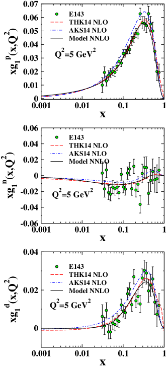
It is worth pointing out in this context that the plots presented above clearly show that the expected statistical accuracies are very good for all analyzed polarized DIS data. This suggests that a reasonable accurate determination of polarized structure function as well as polarized PDFs using Jacobi polynomials expansion approach is possible.
VI Polarized PDFs at the dawn of the RHIC and LHC
The past few years have witnessed tremendous progress in our understanding of the polarized DIS structure functions as well as polarized PDFs. Recent PHENIX measurements on the inclusive production in polarized proton-proton collisions at the Relativistic Heavy Ion Collider (RHIC) at center-of-mass energy of = 510 GeV Adare:2015ozj ; Adare:2014hsq as well as STAR measurements at RHIC on inclusive jet production in polarized proton collisions at = 200 GeV and double spin asymmetries from open charm muon production and leading and next-to-leading order gluon polarization determination in the nucleon at COMPASS Adolph:2012ca , have led to significant improvement in the determination of the polarized gluon distributions especially at small value of deFlorian:2014yva . The new measurements from the PHENIX experiments at RHIC on longitudinal single-spin asymmetries in W± and Z boson production collisions at center of mass energies of =500 and 510 GeV Adare:2015gsd ; Adamczyk:2014xyw are also yielding better constraints on the polarization of sea quarks and anti-quarks.
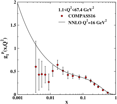
Recently, COMPASS collaborations at CERN collected a large number of events of polarized inelastic scattering and presented their results for the proton longitudinal spin structure functions and the double spin asymmetry Adolph:2015saz . These data collected at center-of-mass energy of = 200 GeV which is the first data covers a very low values of . The statistical precision of improved in the region . The mentioned data covers the range of . The results of the QCD fits to the polarized proton structure function as a functions of and for mean value of Q2 = 16 GeV2 is illustrated in Fig. 15. The solid curve represents our best-fit at NNLO approximation accuracy of perturbative QCD. The data are taken from recent COMPASS16 measurements Adolph:2015saz . Note that the values of Q2 for each measured point are different. The proposed high luminosity and high energy Electron-Ion collider (EIC) such as eRHIC Aschenauer:2014cki ; Miller:2015tjf and EIC@HIAF Yang:2013yeb can probe a broad Q2 < 1 GeV2-range, where one can check the predicted behavior of g at this region. The improved accuracy and the kinematic coverage of the future RHIC data form PHENIX and STAR can lead to more precise polarized PDFs determination in common global QCD analysis of world data. In addition, the accuracy of present determination of polarized PDFs especially polarized gluon distribution still require a widening of the kinematic coverage at small which can be achieved at EIC Accardi:2012qut . Many new and important results reported by these experiments can change substantially our perception of the gluon helicity distribution. For the future, there are more new and precise data to be included. This will lead us to produce fully updated NLO and NNLO polarized PDFs with uncertainties. However, until this major update can be finalized, the NNLO polarized PDFs outlined in this note will serve the only set currently available at NNLO.
VII Summary and conclusions
In this comparative study, we wish to present for the first time a NNLO polarized PDFs analysis of the inclusive world data for , and including the recently published COMPASS16 spin-dependent proton structure function. To establish a meaningful baseline for estimating the impact of these DIS data, we also revisited our next-to-leading order QCD analysis. We have used the Jacobi polynomials expansion method to facilitate the analysis. Overall a very good description of the global inclusive polarized DIS data set has been obtained in our fits over the entire range of Q2 and in which covered by the data. Within this range, it is observed that the Jacobi polynomials approach are more consistent with other methods in the literature. In this paper, the small- behavior of polarized gluon distribution is examined by using the recent DIS data which cover a very low values of especially the very recent high-precision measurements from COMPASS16. The striking feature of obtained polarized gluon distribution is its positivity throughout and clearly away from zero in the regime . Overall, we see that the improvement in the determination of the polarized gluon distribution at NNLO approximation is minor due to the lack of polarized DIS data which cover a wide range of , especially at small . However, there is some indication that the biggest change in going from NLO to NNLO is in the polarized gluon distribution. For total quark and gluon polarized distributions the obtained uncertainties are slightly smaller, and it must be remembered that we use the higher order corrections and more constraining data for . A complete understanding of the origin of the proton spin is still lacking and the uncertainties of the polarized gluon PDF at low value of remain large compared to the currently probed region. In the future, the current analysis will be extended to include the target mass corrections and higher twist effects. The semi-inclusive DIS asymmetries also can be included which can place constraints on the sea quark polarization.
Acknowledgments
We acknowledge helpful conversations and useful discussions with A. Vogt. The authors also would like to thank E. Leader for carefully reading the manuscript and fruitful discussion and critical remarks. We are also grateful to S. Taheri Monfared and F. Arbabifar for useful comments and for providing us with the best fit of THK14 and AKS14 polarized PDFs. F. Taghavi-Shahri acknowledges Ferdowsi University of Mashhad for provided facilities to do this research. This work is supported by Ferdowsi University of Mashhad under Grant No 2/39016, 1394/09/25. H. Khanpour is indebted the University of Science and Technology of Mazandaran and the School of Particles and Accelerators, Institute for Research in Fundamental Sciences (IPM), to support financially this project.
Appendix A: FORTRAN package of our NLO and NNLO polarized PDFs
A FORTRAN package containing our polarized PDFs and their uncertainties at NLO and NNLO approximation as well as the polarized structure functions for the proton, neutron and deuteron can be obtained via Email from the authors upon request. This package includes an example program to illustrate the use of the routines.
References
- (1) E. R. Nocera et al. [NNPDF Collaboration], Nucl. Phys. B 887, 276 (2014).
- (2) E. R. Nocera, Phys. Lett. B 742, 117 (2015).
- (3) P. Jimenez-Delgado et al. [Jefferson Lab Angular Momentum (JAM) Collaboration], Phys. Lett. B 738, 263 (2014).
- (4) P. Jimenez-Delgado, A. Accardi and W. Melnitchouk, Phys. Rev. D 89, no. 3, 034025 (2014).
- (5) F. Arbabifar, A. N. Khorramian and M. Soleymaninia, Phys. Rev. D 89, no. 3, 034006 (2014).
- (6) S. Taheri Monfared, Z. Haddadi and A. N. Khorramian, Phys. Rev. D 89, no. 7, 074052 (2014) [Phys. Rev. D 89, no. 11, 119901 (2014)].
- (7) N. N. K. Borah and D. K. Choudhury, Adv. High Energy Phys. 2014, 1 (2014).
- (8) A. N. Khorramian, S. Atashbar Tehrani, S. Taheri Monfared, F. Arbabifar and F. I. Olness, Phys. Rev. D 83, 054017 (2011).
- (9) J. Blumlein and H. Bottcher, Nucl. Phys. B 841, 205 (2010).
- (10) E. Leader, A. V. Sidorov and D. B. Stamenov, Phys. Rev. D 91, no. 5, 054017 (2015).
- (11) E. C. Aschenauer, R. Sassot and M. Stratmann, Phys. Rev. D 92, no. 9, 094030 (2015).
- (12) J. Ashman et al. [European Muon Collaboration], Phys. Lett. B 206, 364 (1988).
- (13) J. Ashman et al. [European Muon Collaboration], Nucl. Phys. B 328, 1 (1989).
- (14) C. Adolph et al. [COMPASS Collaboration], Phys. Lett. B 753, 18 (2016).
- (15) COMPASS Collaboration, M. Alekseev et al., Phys.Lett. B660, 458 (2008) .
- (16) COMPASS Collaboration, M. Alekseev et al., Eur.Phys.J. C64 , 171 (2009).
- (17) COMPASS Collaboration, C. Adolph et al., Phys.Lett. B718, 922 (2013).
- (18) COMPASS Collaboration, C. Adolph et al., Phys.Rev. D87, 052018 (2013).
- (19) HERMES Collaboration, A. Airapetian et al., Phys.Rev. D71, 012003 (2005)
- (20) A. Airapetian et al. [HERMES Collaboration], Phys. Rev. D 75, 012007 (2007).
- (21) HERMES Collaboration, A. Airapetian et al., JHEP 1008, 130 (2010).
- (22) PHENIX Collaboration, A. Adare et al., Phys.Rev. D79, 012003 (2009).
- (23) PHENIX Collaboration, A. Adare et al., Phys.Rev.Lett. 103, 012003 (2009).
- (24) A. Adare et al. [PHENIX Collaboration], Phys. Rev. D 90, no. 1, 012007 (2014).
- (25) PHENIX Collaboration, A. Adare et al., Phys.Rev. D84, 012006 (2011).
- (26) PHENIX Collaboration, A. Adare et al., Phys.Rev.Lett. 106, 062001 (2011).
- (27) STAR Collaboration, L. Adamczyk et al., Phys.Rev. D89, 012001 (2014).
- (28) STAR Collaboration, L. Adamczyk et al., Phys.Rev. D86, 032006 (2012).
- (29) L. Adamczyk et al. [STAR Collaboration], Phys. Rev. Lett. 115, no. 9, 092002 (2015).
- (30) STAR Collaboration, M. Aggarwal et al., Phys.Rev.Lett. 106, 062002 (2011).
- (31) L. Adamczyk et al. [STAR Collaboration], Phys. Rev. Lett. 113, 072301 (2014).
- (32) J. Blumlein and H. Bottcher, Nucl. Phys. B 636 , 225 (2002).
- (33) M. Gluck, E. Reya, M. Stratmann and W. Vogelsang, Phys. Rev. D 63, 094005 (2001).
- (34) E. Leader, A. V. Sidorov and D. B. Stamenov, Phys. Rev. D 73 , 034023 (2006).
- (35) E. Leader, A. V. Sidorov and D. B. Stamenov, Phys. Rev. D 75, 074027 (2007)
- (36) D. de Florian, G. A. Navarro and R. Sassot, Phys. Rev. D 71, 094018 (2005) .
- (37) Y. Goto et al. [Asymmetry Analysis collaboration], Phys. Rev. D 62 , 034017 (2000), M. Hirai, S. Kumano and N. Saito [Asymmetry Analysis Collaboration], Phys. Rev. D 69 , 054021 (2004).
- (38) M. Hirai and S. Kumano [Asymmetry Analysis Collaboration], Nucl. Phys. B 813, 106 (2009).
- (39) D. de Florian, R. Sassot, M. Stratmann and W. Vogelsang, Phys. Rev. Lett. 101, 072001 (2008).
- (40) D. de Florian, R. Sassot, M. Stratmann and W. Vogelsang, Phys. Rev. D 80, 034030 (2009).
- (41) S. Moch, J. A. M. Vermaseren and A. Vogt, Nucl. Phys. B 889, 351 (2014)
- (42) A. Cafarella, C. Coriano and M. Guzzi, Nucl. Phys. B 748, 253 (2006).
- (43) B. Lampe and E. Reya, Phys. Rept. 332, 1 (2000).
- (44) E. B. Zijlstra and W. L. van Neerven, Nucl. Phys. B 417, 61 (1994) [Nucl. Phys. B 426, 245 (1994)] [Nucl. Phys. B 773, 105 (2007)].
- (45) A. N. Khorramian, H. Khanpour and S. A. Tehrani, Phys. Rev. D 81, 014013 (2010).
- (46) A. N. Khorramian and S. A. Tehrani, Phys. Rev. D 78, 074019 (2008).
- (47) S. Atashbar Tehrani and A. N. Khorramian, JHEP 0707, 048 (2007).
- (48) I. S. Barker, B. R. Martin and G. Shaw, Z. Phys. C 19, 147 (1983).
- (49) I. S. Barker and B. R. Martin, Z. Phys. C 24, 255 (1984).
- (50) V. G. Krivokhizhin, S. P. Kurlovich, V. V. Sanadze, I. A. Savin, A. V. Sidorov and N. B. Skachkov, Z. Phys. C 36, 51 (1987).
- (51) V. G. Krivokhizhin, S. P. Kurlovich, R. Lednicky, S. Nemecek, V. V. Sanadze, I. A. Savin, A. V. Sidorov and N. B. Skachkov, Z. Phys. C 48, 347 (1990).
- (52) J. Chyla and J. Rames, Z. Phys. C 31, 151 (1986).
- (53) I. S. Barker, C. S. Langensiepen and G. Shaw, Nucl. Phys. B 186, 61 (1981).
- (54) A. L. Kataev, A. V. Kotikov, G. Parente and A. V. Sidorov, Phys. Lett. B 417, 374 (1998).
- (55) S. I. Alekhin and A. L. Kataev, Phys. Lett. B 452, 402 (1999).
- (56) A. L. Kataev, G. Parente and A. V. Sidorov, Nucl. Phys. B 573, 405 (2000).
- (57) A. L. Kataev, G. Parente and A. V. Sidorov, Phys. Part. Nucl. 34, 20 (2003) [Fiz. Elem. Chast. Atom. Yadra 34, 43 (2003)] [Phys. Part. Nucl. 38, no. 6, 827 (2007)].
- (58) A. L. Kataev, JETP Lett. 81, 608 (2005) [Pisma Zh. Eksp. Teor. Fiz. 81, 744 (2005)].
- (59) E. Leader, A. V. Sidorov and D. B. Stamenov, Int. J. Mod. Phys. A 13, 5573 (1998).
- (60) K. A. Olive et al. [Particle Data Group Collaboration], Chin. Phys. C 38, 090001 (2014).
- (61) Y. L. Dokshitzer, Sov. Phys. JETP 46, 641 (1977) [Zh. Eksp. Teor. Fiz. 73, 1216 (1977)].
- (62) V. N. Gribov and L. N. Lipatov, Sov. J. Nucl. Phys. 15, 438 (1972) [Yad. Fiz. 15, 781 (1972)].
- (63) L. N. Lipatov, Sov. J. Nucl. Phys. 20, 94 (1975) [Yad. Fiz. 20, 181 (1974)].
- (64) G. Altarelli and G. Parisi, Nucl. Phys. B 126, 298 (1977).
- (65) K. Abe et al. [E143 Collaboration], Phys. Rev. D 58, 112003 (1998).
- (66) A. Airapetian et al. [HERMES Collaboration], Phys. Lett. B 442 (1998) 484.
- (67) B. Adeva et al. [Spin Muon Collaboration], Phys. Rev. D 58, 112001 (1998).
- (68) J. Ashman et al. [European Muon Collaboration], Phys. Lett. B 206 (1988) 364; J. Ashman et al. [European Muon Collaboration], Nucl. Phys. B 328 , 1 (1989).
- (69) P. L. Anthony et al. [E155 Collaboration], Phys. Lett. B 493 , 19 (2000).
- (70) A. Airapetian et al. [HERMES Collaboration], Phys. Rev. D 75 , 012007 (2007).
- (71) M. G. Alekseev et al. [COMPASS Collaboration], Phys. Lett. B 690, 466 (2010).V. Y. Alexakhin et al. [COMPASS Collaboration], Phys. Lett. B 647 , 8 (2007).
- (72) P. L. Anthony et al. [E155 Collaboration], Phys. Lett. B 463 , 339 (1999).
- (73) E. S. Ageev et al. [COMPASS Collaboration], Phys. Lett. B 612, 154 (2005).
- (74) V. Y. .Alexakhin et al. [COMPASS Collaboration], Phys. Lett. B 647, 8 (2007).
- (75) P. L. Anthony et al. [E142 Collaboration], Phys. Rev. D 54 , 6620 (1996).
- (76) K. Abe et al. [E154 Collaboration], Phys. Rev. Lett. 79 , 26 (1997).
- (77) K. Ackerstaff et al. [HERMES Collaboration], Phys. Lett. B 404 , 383 (1997).
- (78) X. Zheng et al. [Jefferson Lab Hall A Collaboration], Phys. Rev. C 70, 065207 (2004).
- (79) K. Kramer, D. S. Armstrong, T. D. Averett, W. Bertozzi, S. Binet, C. Butuceanu, A. Camsonne and G. D. Cates et al., Phys. Rev. Lett. 95, 142002 (2005).
- (80) H. Khanpour and S. A. Tehrani, Phys. Rev. D 93, 014026 (2016).
- (81) S. Atashbar Tehrani, Phys. Rev. C 86 , 064301 (2012) .
- (82) A. D. Martin, R. G. Roberts, W. J. Stirling and R. S. Thorne, Eur. Phys. J. C 28, 455 (2003).
- (83) J. Pumplin, D. Stump et al., Phys. Rev. D 65 , 014013 (2001).
- (84) S. T. Monfared, A. N. Khorramian and S. A. Tehrani, J. Phys. G 39, 085009 (2012).
- (85) F. James, “MINUIT Function Minimization and Error Analysis: Reference Manual Version 94.1,” CERN-D-506.
- (86) R. D. Ball et al. [NNPDF Collaboration], Phys. Lett. B 728, 524 (2014).
- (87) R. D. Ball et al. [NNPDF Collaboration], Nucl. Phys. B 874, 36 (2013).
- (88) N. Sato et al. [Jefferson Lab Angular Momentum Collaboration], Phys. Rev. D 93, no. 7, 074005 (2016).
- (89) A. D. Martin, R. G. Roberts, W. J. Stirling and R. S. Thorne, Eur. Phys. J. C 35, 325 (2004).
- (90) D. de Florian, R. Sassot, M. Stratmann and W. Vogelsang, Prog. Part. Nucl. Phys. 67, 251 (2012).
- (91) D. de Florian, R. Sassot, M. Stratmann and W. Vogelsang, Phys. Rev. Lett. 113, no. 1, 012001 (2014).
- (92) M. Lacombe, B. Loiseau, R. Vinh Mau, J. Cote, P. Pires and R. de Tourreil, Phys. Lett. B 101, 139 (1981).
- (93) R. Machleidt, K. Holinde and C. Elster, Phys. Rept. 149, 1 (1987).
- (94) J. F. Owens, A. Accardi and W. Melnitchouk, Phys. Rev. D 87, no. 9, 094012 (2013).
- (95) H. Khanpour, A. N. Khorramian and S. A. Tehrani, J. Phys. G 40, 045002 (2013).
- (96) J. Blümlein, H. Böttcher and A. Guffanti, Nucl. Phys. B 774, 182 (2007).Nucl. Phys. Proc. Suppl. 135, 152 (2004).
- (97) S. Alekhin, J. Blümlein, S. Klein and S. Moch, Phys. Rev. D 81, 014032 (2010).
- (98) M. Glück, E. Reya and C. Schuck, Nucl. Phys. B 754, 178 (2006).P. Jimenez-Delgado and E. Reya, Phys. Rev. D 79, 074023 (2009).
- (99) A. D. Martin, W. J. Stirling, R. S. Thorne and G. Watt, Eur. Phys. J. C 64, 653 (2009).
- (100) H1 and ZEUS collab.F. D. Aaron et al. JHEP 1001, 109 (2010).
- (101) D. d’Enterria and P. Z. Skands, arXiv:1512.05194 [hep-ph].
- (102) A. Adare et al. [PHENIX Collaboration], Phys. Rev. D 93, no. 1, 011501 (2016).
- (103) A. Adare et al. [PHENIX Collaboration], arXiv:1504.07451 [hep-ex].
- (104) E. C. Aschenauer et al., arXiv:1409.1633 [physics.acc-ph].
- (105) G. A. Miller, M. D. Sievert and R. Venugopalan, arXiv:1512.03111 [nucl-th].
- (106) J. C. Yang et al., Nucl. Instrum. Meth. B 317, 263 (2013).
- (107) A. Accardi et al., arXiv:1212.1701 [nucl-ex].