Wave fronts and cascades of soliton interactions in the periodic two dimensional Volterra system

Abstract

In the paper we develop the dressing method for the solution of the two-dimensional periodic Volterra system with a period $N$. We derive soliton solutions of arbitrary rank $k$ and give a full classification of rank $1$ solutions. We have found a new class of exact solutions corresponding to wave fronts which represent smooth interfaces between two nonlinear periodic waves or a periodic wave and a trivial (zero) solution. The wave fronts are non-stationary and they propagate with a constant average velocity. The system also has soliton solutions similar to breathers, which resembles soliton webs in the KP theory. We associate the classification of soliton solutions with the Schubert decomposition of the Grassmanians ${\rm Gr}_{\mathbb{R}}(k,N)$ and ${\rm Gr}_{\mathbb{C}}(k,N)$.

1 Introduction

Construction of explicit exact solutions for integrable systems is an important and well developed area of research. There is a variety of methods designed to tackle this problem and vast literature concerning soliton solutions of rank one. In this paper we develop the dressing method in application to a periodic two-dimensional Volterra system and derive explicitly soliton solutions of arbitrary rank. We found solutions resembling breathers (in the theory of the sine-Gordon equation), nonlinear periodic waves and a new type of exact solution for integrable systems, which are smooth interfaces between two nonlinear periodic waves or a periodic wave and a trivial (zero) solution.

The dressing method for Lax integrable systems was originally formulated and developed in [1, 2]. Its predecessor was proposed by Bargmann (1949) [3], where the author performed the dressings of the Schrödinger operator and discovered potentials, which now we would associate with the profiles of one and two soliton solutions for the Korteweg de–Vries (KdV) equation. The connection of the potentials of the Schrödinger operators with solutions of the KdV equation was established much later by Gardner, Greene, Kruskal and Miura, who discovered the inverse spectral transform [4]. A year later an elegant interpretation of their results was given by Lax in [5], where the concept of Lax pair has first appeared.

In this paper, we develop the dressing method and study exact solutions for the $2$–dimensional generalisation of the periodic Volterra lattice [6, 7]

$$\left\{\begin{array}[]{ll}\phi^{(i)}_{t}=\theta^{(i)}_{x}+\theta^{(i)}\phi^{(i)}_{x}-e^{2\phi^{(i-1)}}+e^{2\phi^{(i+1)}},&\phi^{(i+N)}=\phi^{(i)},\quad\theta^{(i+N)}=\theta^{(i)},\\ &\\ \theta^{(i+1)}-\theta^{(i)}+\phi^{(i+1)}_{x}+\phi^{(i)}_{x}=0,&\sum_{i=1}^{N}\phi^{(i)}=\sum_{i=1}^{N}\theta^{(i)}=0,\end{array}\right..$$ (4)

System (4) can be regarded as an integrable discretisation of the Kadomtsev-Petviashvili (KP) equation (see Section 3.3). The KP equation, originally derived for ion-acoustic waves of small amplitude in plasma [8], is a $2+1$–dimensional integrable generalisation of the KdV equation. Its mathematical theory made a deep impact to the theory of integrable equations and give rise to useful notions such as $\tau$ function and Sato Grassmanian [9]. The KP equation possesses a rich set of exact solutions, whose classification require advanced techniques from cluster algebra, tropical geometry and combinatorics developed in [10, 11, 12].

Equation (4) was first derived in 1979 motivated by the reduction group theory for Lax representation [6]. For a fixed period $N$, the variables $\theta^{(i)}$ can be eliminated and thus (4) can be rewritten as a system of $(N-1)$-component second order evolutionary equations. In the simplest nontrivial case $N=3$, the system (4) becomes

$$\left\{\begin{array}[]{l}3\phi^{(1)}_{t}=\phi^{(1)}_{xx}+2\phi^{(2)}_{xx}+2\phi^{(1)}_{x}\phi^{(2)}_{x}+{\phi^{(1)}_{x}}^{2}+3e^{2\phi^{(2)}}-3e^{-2\phi^{(1)}-2\phi^{(2)}}\\ 3\phi^{(2)}_{t}=-2\phi^{(1)}_{xx}-\phi^{(2)}_{xx}-2\phi^{(1)}_{x}\phi^{(2)}_{x}-{\phi^{(2)}_{x}}^{2}-3e^{2\phi^{(1)}}+3e^{-2\phi^{(1)}-2\phi^{(2)}}\end{array}\right.$$ (7)

and after a point transformation it takes the form of a nonlinear Schrödinger type equation (system “u4” in [13])

$$iu_{T}=u_{XX}+(u_{X}^{\star})^{2}+e^{-2u-2u^{\star}}+\omega^{\star}e^{-2\omega u-2\omega^{\star}u^{\star}}+\omega e^{-2\omega^{\star}u-2\omega u^{\star}},\quad\omega=e^{\frac{2\pi i}{3}}\,,$$

where $\star$ denotes complex conjugation. In this case, the system is bi-Hamiltonian. A recursion operator and bi-Hamiltonian structure for system (7) are explicitly constructed from its Lax representation in [14]. A certain class of Darboux transformations for arbitrary fixed period $N$ has recently been constructed in [15].

For infinite $N$, equation (4) is an integrable differential-difference equation in $2+1$ dimensions. It appeared in [16] where the authors classified a family of equations with the non-locality of intermediate long wave type. Its infinitely many symmetries and conserved densities are constructed using its master symmetry in [17].

Bargmann’s potentials correspond to a rational (in the wave number) factor to the Jost function [3]. In the dressing method we also start with a rational in the spectral parameter $\lambda$ matrix factor $\Phi(\lambda)$, which modifies the fundamental solution of the “undressed” Lax pair. In the case of system (4) the Lax operators contain $N\times N$ matrices and are invariant with respect to a reduction group isomorphic to ${\mathbb{Z}}_{2}\times{\mathbb{D}}_{N}$. We construct the reduction group invariant dressing factors $\Phi(\lambda)$ which have $N$ or $2N$ simple poles belonging to the orbits generated by transformations $\lambda\mapsto\omega\lambda,\ \lambda\mapsto\lambda^{*}$, where $\omega=\exp(\frac{2\pi i}{N})$. The case of $N$ simple poles leads to a new class of solutions, which we call kink solutions, while solutions corresponding to the orbits with $2N$ poles we call breathers. This terminology is borrowed from the sine-Gordon theory where a kink solution corresponds to a dressing factor with one pole and two poles factor leads to a breather solution [18, 19]. We could also construct $(n,m)$ multisoliton solutions with $n$ kinks and $m$ breathers, but this generalisation is rather straightforward and therefore in this paper we focus on solutions corresponding to a single orbit (i.e. one kink and one breather solutions).

A kink solution can be parametrised by a real number $\nu\notin\{\pm 1,0\}$ and a point on a real Grassmannian ${\rm Gr}_{\mathbb{R}}(k,N)$, while a breather solution can be uniquely parametrised by a complex number $\mu\in{\mathbb{C}}$ such that $|\mu|\notin\{1,0\},\ \mbox{Im}\,\mu^{N}\neq 0$ and a point on a complex Grassmannian ${\rm Gr}_{\mathbb{C}}(k,N)$. The number $k$ in ${\rm Gr}(k,N)$ is the rank of the soliton solution. There is a difference between the cases of even and odd $N$. When $N$ is even, there are two different orbits with $N$ points, namely $\{\nu\omega^{k}\}_{k=1}^{N}$ and $\{\nu\omega^{k+\frac{1}{2}}\}_{k=1}^{N}$. They results in two different kink solutions. A fine classification of wave interfaces (in the kink case) and soliton interactions (in the breather case) can be naturally given in the terms of the invariant Schubert cell decomposition of the Grassmannian. In particular, elementary line breathers and periodic kink solutions correspond to one-dimensional invariant Schubert cells of the Grassmannians.

Kink solutions represent regions filled by non-linear periodic waves with moving interfaces between the regions, see Figure 1. Thus we also call them wave fronts.

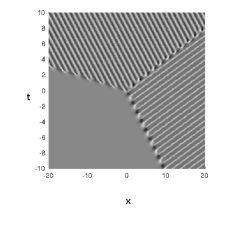
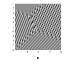
Figure 1: Density plots of $\phi^{(1)}(x,t)$ for $N=5$ of rank 1 and rank 2 kink solutions

Breathers correspond to a cascade of soliton decays and fusions. The density plots of a breather solution in the $(x,t)$-plane resemble soliton webs of the KP equations in the $(x,y)$-plane for a fixed moment of time, see Figure 2.

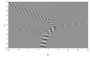
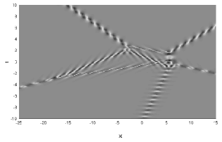
Figure 2: Density plots of $\phi^{(1)}(x,t)$ for $N=5$ of rank 1 and rank 2 breather solutions

In the paper we give explicit and detailed derivation for these two types of soliton solutions of arbitrary rank for the two dimensional Volterra system (4) and give a complete classification of rank $1$ kink and breather solutions.

The arrangement of this paper is as follows: In Section 2, we recall the Lax representation for equation (4) and its reduction group. In Section 3, we discuss the dressing method in the presence of the reduction group. We explicitly derive both kink and breather solutions for equation (4) on the trivial background using the dressing method. All exact solutions emerging from the dressing method can be written in the form

$$\phi^{(i)}=\frac{1}{2}\ln\frac{\tau_{i-1}\tau_{i+1}}{\tau_{i}^{2}}.$$ (8)

Under a certain continuous limit $N\to\infty$, equation (4) converges to the well known KP equation. In this limit $\tau_{i}$ in (8) can be related to the Hirota $\tau$-function for the bilinear form of the KP equation [20]. In Section 4, we classify both kink and breather solutions of rank $1$ according to the eigenspaces of the constant matrix $\Delta$ in the Lax operators of equation (4). For rank $1$ kink solutions, we start with a description of all possible rank 1 kink solutions in the cases of $N=3,4$ and further prove the general results for arbitrary dimensions. For rank $1$ breather solutions we present some typical configurations and the general result on the number of possible distinct configurations. Our definition soliton graphs based on tropicalisation is motivated by [10] although we do not have structure associated with Wronskian of solutions. In the Conclusion we summarise our results and discuss the feasibility of a full classification of higher rank solutions.

2 Lax representation and the dihedral reduction group

Let us consider general matrix operators of the form

$$\hat{L}(\lambda)=D_{x}+\mathbf{X}(x,t,\lambda),\qquad\hat{M}(\lambda)=D_{t}+\mathbf{T}(x,t,\lambda),$$ (9)

where $D_{x}$ and $D_{t}$ are total derivatives in $x$ and $t$ respectively, $\lambda\in{\mathbb{C}}$ is a spectral parameter, $\mathbf{X}$ and $\mathbf{T}$ are $N\times N$ traceless matrices

$$\mathbf{X}(x,t,\lambda) = \mathbf{X}_{0}+\lambda^{-1}\mathbf{U}+\lambda\overline{\mathbf{U}}$$

$$\mathbf{T}(x,t,\lambda) = \mathbf{T}_{0}+\lambda^{-1}\mathbf{A}+\lambda\overline{\mathbf{A}}+\lambda^{-2}\mathbf{B}+\lambda^{2}\overline{\mathbf{B}}$$

and the matrices $\mathbf{X}_{0},\mathbf{U},\overline{\mathbf{U}},\mathbf{T}_{0},\mathbf{A},\overline{\mathbf{A}},\mathbf{B}$ and $\overline{\mathbf{B}}$ are functions of $x$ and $t$. The compatibility condition $[\hat{L},\hat{M}]=0$, that is,

$$\mathbf{T}_{x}-\mathbf{X}_{t}+[\mathbf{X},\mathbf{T}]=0$$ (10)

gives $7(N^{2}-1)$ partial differential equations (coefficients of $\lambda^{-3},\ldots,\lambda^{3}$) for $7N^{2}$ matrix entries.

We define a group of automorphisms generated by the following two transformations for an operator ${\bf d}(\lambda)$: the first one is

$${\iota}:{\bf d}(\lambda)\mapsto-{\bf d}^{\dagger}(\lambda^{-1}),$$ (11)

where ${\bf d}^{\dagger}$ is the adjoint operator of operator ${\bf d}$. The second one is

$$s:{\bf d}(\lambda)\mapsto Q{\bf d}(\omega^{-1}\lambda)Q^{-1},\qquad Q=\,\mbox{diag}\,(\omega^{i}),\quad\omega=\exp\frac{2\pi{\rm i}}{N}.$$ (12)

These two non-commuting transformations satisfy

$${\iota}^{2}=s^{N}={\rm id},\quad{\iota}s{\iota}=s^{-1}$$

and therefore generate the dihedral group denoted by ${\mathbb{D}}_{N}$. We call the group generated by transformations (11) and (12) the reduction group [6, 7, 21, 22, 23, 24]. Note that the transformation ${\iota}$ (11) is an outer automorphism of the Lie algebra $sl(n)$ over the Laurent polynomial ring $\mathbb{C}[\lambda,\lambda^{-1}]$.

Proposition 1.

If the linear operators (9) are invariant with respect to the reduction group ${\mathbb{D}}_{N}$, then they can be written in the form

$$\hat{L} = D_{x}+\lambda^{-1}\mathbf{u}\Delta-\lambda\Delta^{-1}\mathbf{u}$$ (13)

$$\hat{M} = D_{t}+\lambda^{-1}\mathbf{a}\Delta-\lambda\Delta^{-1}\mathbf{a}+\lambda^{-2}\mathbf{b}\Delta^{2}-\lambda^{2}\Delta^{-2}\mathbf{b}$$ (14)

where $\mathbf{u},\mathbf{a},\mathbf{b}$ are diagonal matrices and $\Delta$ is the shift operator given by

$$\Delta=\begin{pmatrix}0&1&0&\dots&0\\ 0&0&1&\dots&0\\ 0&0&0&\dots&1\\ 1&0&0&\dots&0\end{pmatrix}.$$ (15)

Proof.

It follows from the invariance under the transformation ${\iota}$ (11), that is,

$$(\hat{L}(\lambda),\hat{M}(\lambda))=(-\hat{L}^{\dagger}(\lambda^{-1}),-\hat{M}^{\dagger}(\lambda^{-1})),$$

that

$$\overline{\mathbf{U}}=-\mathbf{U}^{\mbox{tr}},\quad\overline{\mathbf{A}}=-\mathbf{A}^{\mbox{tr}},\quad\overline{\mathbf{B}}=-\mathbf{B}^{\mbox{tr}},\quad\mathbf{X}_{0}=-\mathbf{X}_{0}^{\mbox{tr}},\quad\mathbf{T}_{0}=-\mathbf{T}_{0}^{\mbox{tr}},$$ (16)

where ${}^{\mbox{tr}}$ denotes matrix transposition. The invariance under the transformation $s$ implies that $\mathbf{X}_{0},\mathbf{T}_{0}$ are diagonal and the matrices $\mathbf{U},\mathbf{A}$ and $\mathbf{B}$ are of the form

$$\mathbf{U}=\mathbf{u}\Delta,\quad\mathbf{A}=\mathbf{a}\Delta,\quad\mathbf{B}=\mathbf{b}\Delta^{2},$$

where $\mathbf{u},\mathbf{a}$ and $\mathbf{b}$ are diagonal matrices and $\Delta$ is given by (15). Combining with (16), we get $\mathbf{X}_{0}=\mathbf{T}_{0}=0$ and further the expressions (13) and (14) in the statement. ∎

Let $\mathbf{u}=\,\mbox{diag}\,(u^{(i)}),\mathbf{a}=\,\mbox{diag}\,(a^{(i)})$ and $\mathbf{b}=\,\mbox{diag}\,(b^{(i)})$. Then the compatibility condition of Lax operators (13) and (14) leads to $3N$ equations

$$u^{(i)}b^{(i+1)}-b^{(i)}u^{(i+2)}=0\,,$$ (17)

$$D_{x}(b^{(i)})+u^{(i)}a^{(i+1)}-a^{(i)}u^{(i+1)}=0\,,$$ (18)

$$D_{t}(u^{(i)})=D_{x}(a^{(i)})-u^{(i-1)}b^{(i-1)}+b^{(i)}u^{(i+2)}$$ (19)

in $3N$ variables $u^{(i)},a^{(i)}$ and $b^{(i)}$, where $i=1,\cdots,N$. In this paper we shall assume that all upper indices, taking value from $1$ to $N$, are counted modulo $N$, if not stated otherwise. Take

$$\mathbf{u}=\,\mbox{diag}\,(\exp(\phi^{(1)}),\ldots,\exp(\phi^{(N)}))\,,\quad\mathbf{a}=\,\mbox{diag}\,(\theta^{(1)}\exp(\phi^{(1)}),\ldots,\theta^{(N)}\exp(\phi^{(N)})).$$ (20)

It follows from (17)-(19) that we can set $b^{(i)}=\exp\left(\phi^{(i)}+\phi^{(i+1)}\right)$ and $\sum_{i=1}^{N}\phi^{(i)}=\sum_{i=1}^{N}\theta^{(i)}=0$ without losing generality. In the variables $\phi^{(i)}$ and $\theta^{(i)}$ the system of equations (17)-(19) leads to the 2-dimensional generalisation of the Volterra system (4). The corresponding operators (13) and (14) can be expressed as the invariant operators under the reduction group ${\mathbb{D}}_{N}$, namely,

$$\begin{array}[]{ll}{\cal L}=D_{x}+U,&U=\lambda^{-1}\mathbf{u}\Delta-\lambda\Delta^{-1}\mathbf{u},\\ {\cal M}=D_{t}+V,&V=\lambda^{-2}\mathbf{u}\Delta\mathbf{u}\Delta+\lambda^{-1}\mathbf{a}\Delta-\lambda\Delta^{-1}\mathbf{a}-\lambda^{2}\Delta^{-1}\mathbf{u}\Delta^{-1}\mathbf{u},\end{array}$$ (23)

where $\mathbf{u}$ and $\mathbf{a}$ are defined by (20) and the matrix $\Delta$ is given by (15). The condition of commutativity of these operators

$$[{\cal L},{\cal M}]=D_{x}(V)-D_{t}(U)+[U,V]=0$$ (24)

leads to the $2$–dimensional generalisation of the Volterra lattice (4) [6, 7]. This is often called a zero curvature representation or Lax representation of equation (4). These two operators, ${\cal L}$ and ${\cal M}$, are conventionally called the Lax pair.

If we assume that the functions $\phi^{(k)},\theta^{(k)}$ in (20) are real, then the Lax operators ${\cal L},{\cal M}$ are also invariant with respect to transformation

$$r\,:\,{\cal L}(\lambda)\mapsto{\cal L}^{\star}(\lambda^{\star}),\quad{\cal M}(\lambda)\mapsto{\cal M}^{\star}(\lambda^{\star}),$$ (25)

where ^⋆ means its complex conjugate. This transformation extends the dihedral group. The group generated by $s,{\iota},r$ is isomorphic to ${\mathbb{Z}}_{2}\times{\mathbb{D}}_{N}$.

3 Rational dressing method for the generalised Volterra lattice

In this section, we use the method of rational dressing [1, 2, 7] to construct new exact solutions of (4) starting from a known exact solution. Let us denote by $U_{0},V_{0}$ the matrices $U,V$ in which $\phi^{(i)}$ are replaced by the known exact solution $\phi_{0}^{(i)},i=1,\cdots,N$ of (4), that is,

$$U_{0}=\lambda^{-1}\mathbf{u}_{0}\Delta-\lambda\Delta^{-1}\mathbf{u}_{0},\qquad V_{0}=\lambda^{-2}\mathbf{u}_{0}\Delta\mathbf{u}_{0}\Delta+\lambda^{-1}\mathbf{a}_{0}\Delta-\lambda\Delta^{-1}\mathbf{a}_{0}-\lambda^{2}\Delta^{-1}\mathbf{u}_{0}\Delta^{-1}\mathbf{u}_{0}.$$

The corresponding overdetermined linear system

$${\cal L}_{0}\Psi_{0}=(D_{x}+U_{0})\Psi_{0}=0,\qquad{\cal M}_{0}\Psi_{0}=(D_{t}+V_{0})\Psi_{0}=0$$ (26)

has a common fundamental solution $\Psi_{0}(\lambda,x,t)$. Following [1, 2] we shall assume that the fundamental solution $\Psi(\lambda,x,t)$ for the new (“dressed”) linear problems

$${\cal L}\Psi=(D_{x}+U)\Psi=0,\qquad{\cal M}\Psi=(D_{t}+V)\Psi=0$$ (27)

is of the form

$$\Psi=\Phi(\lambda)\Psi_{0},\quad\det\Phi\not=0,$$ (28)

where the dressing matrix $\Phi(\lambda)$ is assumed to be rational in the spectral parameter $\lambda$ and to be invariant with respect to the symmetries

$$\Phi^{-1}(\lambda^{-1})=\Phi^{\mbox{tr}}(\lambda);$$ (29)

$$Q\Phi(\omega^{-1}\lambda)Q^{-1}=\Phi(\lambda).$$ (30)

Conditions (29) and (30) guarantee that the corresponding Lax operators $\mathcal{L}$ and $\mathcal{M}$ are invariant under transformations (11) and (12).

We are going to derive real solutions for the real equation. Thus we also require

$$\Phi^{\star}(\lambda^{\star})=\Phi(\lambda).$$ (31)

It follows from (26), (27) and (28) that

$$\Phi(D_{x}+U_{0})\Phi^{-1}=U;$$ (32)

$$\Phi(D_{t}+V_{0})\Phi^{-1}=V.$$ (33)

These equations enable us to specify the form of the dressing matrix $\Phi$ and construct the corresponding “dressed” solution $\phi^{(i)}$ of equation (4).

Let us consider the most trivial case when the dressing matrix $\Phi$ does not depend on the spectral parameter $\lambda$. In this case the dressing matrix does not result any new solutions.

Proposition 2.

Assume that $\Phi$ is a $\lambda$ independent dressing matrix for the two dimensional generalisation of the Volterra lattice (4) and $\phi_{0}^{(i)}$ is a real solution. If it satisfies (29)–(31), then the matrix $\Phi=\pm I_{N}$, where $I_{N}$ is the $N\times N$identity matrix and the real solutions on the background $\phi_{0}^{(i)}$ are $\phi^{(i)}=\phi_{0}^{(i)}$.

Proof.

Under the assumption that the dressing matrix $\Phi$ is independent of the spectral parameter $\lambda$, it follows from (32) and (33) that

$$D_{x}\Phi=0;\ D_{t}\Phi=0;\ \Phi\mathbf{u}_{0}\Delta=\mathbf{u}\Delta\Phi;\ \Phi\Delta^{-1}\mathbf{u}_{0}=\Delta^{-1}\mathbf{u}\Phi;\ \Phi\mathbf{a}_{0}\Delta=\mathbf{a}\Delta\Phi;\ \Phi\Delta^{-1}\mathbf{a}_{0}=\Delta^{-1}\mathbf{a}\Phi.$$ (34)

It is obvious that the matrix $\Phi$ is independent of $x$ and $t$. Since $\Phi$ satisfies (29)–(31) , we deduce that matrix $\Phi$ is real, $\Phi\Phi^{\mbox{tr}}=I_{N}$ and $\Phi$ is diagonal. Thus the constant matrix $\Phi$ has $\pm 1$ on the diagonal. Substituting such $\Phi$ into (34), we get $\Phi=\pm I_{N}$ and $\phi^{(i)}=\phi_{0}^{(i)}$ since both $\phi^{(i)}$ and $\phi_{0}^{(i)}$ are real. ∎

A $\lambda$–dependent dressing matrix $\Phi(\lambda)$, which is invariant with respect to the symmetries (29)–(31) has poles at the orbits of the reduction group. Simplest “one soliton” dressing corresponds to the cases when the matrix $\Phi(\lambda)$ has only simple poles belonging to a single orbit.

Notice that if $\Phi(\lambda)$ is invariant under the reduction group, so is $\Phi^{-1}(\lambda)$. Instead of specifying the poles for $\Phi(\lambda)$, we first specify the poles for $\Phi^{-1}$, and then determine $\Phi$ from the relation (29). If $\Phi^{-1}(\lambda)$ has a pole at the point $\mu$, then by the second relation (30) (for $\Phi^{-1}$) it must also have poles at the points $\omega^{-1}\mu$, $\omega^{-2}\mu$, $\dots$, $\omega^{-(N-1)}\mu$. Due to (31), there are two non-trivial cases:

1. The matrix $\Phi^{-1}(\lambda)$ has $N$ poles:

   • for arbitrary $N$ poles at $\omega^{-k}\mu,\ k=0,\cdots,N-1,\ \mu\neq 0,\ \mu\neq\pm 1,\ \mu=\mu^{\star};$

   • when $N$ is even, i.e. $N=2m$, poles at $\omega^{-k}\mu,\ k=0,\cdots,N-1,\ \mu=\nu\exp(\frac{\pi{\rm i}}{N}),\nu\in{\mathbb{R}},\nu\notin\{\pm 1,0\};$

2. The matrix $\Phi^{-1}(\lambda)$ has $2N$ complex poles at $\omega^{-k}\mu$ and $\omega^{-k}\mu^{\star}$, where $k=0,\cdots,N-1$ and

   $$\mu\in{\mathbb{C}},\ |\mu|\neq 1,\ \mu\neq\omega^{k}\mu^{\star},\ k=1,\ldots,N.$$

Note that when $N=2m+1$ is odd, the case (i) in (1) includes the case (ii) since

$$\omega^{n}\mu=\omega^{l}\nu\exp(\frac{\pi{\rm i}}{N})=-\nu\in{\mathbb{R}}.$$

The extra conditions on $\mu$ is to ensure that the poles for $\Phi$ and $\Phi^{-1}$ are distinct. These cases correspond to the “kink” and “breather” solutions respectively.

The explicit forms of the matrix $\Phi^{-1}(\lambda)$ corresponding the above two cases and invariant with respect to the symmetries (30) and (31) are

$$({\rm 1}) ({\rm i})\ \ \Phi^{-1}(\lambda)=C+\sum_{k=0}^{N-1}\frac{Q^{-k}AQ^{k}}{\lambda\omega^{k}-\mu},\quad A=A^{\star},\quad\mu=\mu^{\star},\ \mu\neq 0,\ \mu\neq\pm 1;$$

$$({\rm ii})\ \ \Phi^{-1}(\lambda)=C+\sum_{k=0}^{2m-1}\frac{Q^{-k}AQ^{k}}{\lambda\omega^{k}-\mu},\quad N=2m,\ A^{\star}=\omega^{-1}Q^{-1}AQ,\ \mu=\nu\exp(\frac{\pi{\rm i}}{2m}),\ \nu\in{\mathbb{R}},\nu\notin\{\pm 1,0\};$$

$$({\rm 2}) \Phi^{-1}(\lambda)=C+\sum_{k=0}^{N-1}\left(\frac{Q^{-k}AQ^{k}}{\lambda\omega^{k}-\mu}+\frac{Q^{-k}A^{\star}Q^{k}}{\lambda\omega^{k}-\mu^{\star}}\right),\quad|\mu|\neq 1,\ \mu\neq\omega^{k}\mu^{\star},\ k=1,\ldots,N,$$

where $C$ and $A$ are $\lambda$-independent matrices of size $N\times N$. Moreover, to satisfy (30) and (31), we have $C=QCQ^{-1}$ implying $C$ is diagonal and $C=C^{\star}$. Hence we assume that

$$C=\,\mbox{diag}\,(c_{1},\cdots,c_{N}),$$ (35)

where $c_{i},i=1,\cdots,N$ are real functions of $x$ and $t$.

We now derive the conditions on the matrices $A$ and $C$ such that $\Phi^{-1}(\lambda)$ satisfies (29). In this case, we have $\Phi(\lambda)=\left(\Phi^{-1}(\lambda^{-1})\right)^{\mbox{tr}}$. It follows that

$$({\rm 1}) \Phi(\lambda)=C+\sum_{k=0}^{N-1}\frac{Q^{k}A^{\mbox{tr}}Q^{-k}}{\lambda^{-1}\omega^{k}-\mu},\quad A=A^{\star},\ \mu=\mu^{\star},\mbox{or}\ N=2m,\ \mu=\nu\exp(\frac{\pi{\rm i}}{N}),A^{\star}=\omega^{-1}Q^{-1}AQ;$$ (36)

$$({\rm 2}) \Phi(\lambda)=C+\sum_{k=0}^{N-1}\left(\frac{Q^{k}A^{\mbox{tr}}Q^{-k}}{\lambda^{-1}\omega^{k}-\mu}+\frac{Q^{k}A^{\star\mbox{tr}}Q^{-k}}{\lambda^{-1}\omega^{k}-\mu^{\star}}\right).$$ (37)

Proposition 3.

Let $I_{N}$ denote the $N\times N$ identity matrix. The dressing matrix satisfies (29) if and only if matrix $A$ and the real diagonal matrix $C$ satisfy the relations:

$$\lim_{\lambda\to\infty}\Phi(\lambda)=C^{-1};\qquad\Phi(\mu)A=0.$$ (38)

Proof.

We verify that the above $\Phi(\lambda)$ is indeed the inverse matrix of $\Phi^{-1}(\lambda)$ by checking $\Phi(\lambda)\Phi^{-1}(\lambda)=I_{N}$. The product is a rational matrix function of $\lambda$. Taking the limit at $\lambda=\infty$ we obtain $\lim_{\lambda\to\infty}\Phi(\lambda)C=I_{N}$, which implies the first equation in (38). Under the assumptions on $\mu$, the poles of both $\Phi$ and $\Phi^{-1}$ are simple and distinct. Therefore, $\Phi(\lambda)\Phi^{-1}(\lambda)$ has $2N$ simple poles. Requesting the vanishing of the residue at $\lambda=\mu$ we obtain the second equation in (38). The residues at all other points of the reduction group orbit will vanish due to the manifest invariants of the expression with respect to the reduction group. ∎

We now investigate the conditions (32) and (33) for $\Phi(\lambda)$ which follow from the fact that it is a dressing matrix. Notice that $\Phi,U_{0}$ and $\Phi^{-1}$ have distinct simple poles. Thus the left hand side of (32) has simple poles only. We first compare the residues at the pole $\mu$. It follows that

$$\lim_{\lambda\to\mu}(\lambda-\mu)\Phi(D_{x}+U_{0}(\lambda))\Phi^{-1}=\Phi(\mu)(D_{x}+U_{0}(\mu))A=0.$$ (39)

Thus $(D_{x}+U_{0}(\mu))A\in\ker\Phi(\mu)$. In a similar way it follows from the condition (33) that

$$\Phi(\mu)(D_{t}+V_{0}(\mu))A=0,\quad\mbox{that is},\quad(D_{t}+V_{0}(\mu))A\in\ker\Phi(\mu).$$ (40)

We compute the residue at $\lambda=\infty$ of both sides of (32) and we have

$$\lim_{\lambda\to\infty}\frac{1}{\lambda}\Phi(\lambda)(D_{x}+U_{0}(\lambda))\Phi^{-1}(\lambda)=-\lim_{\lambda\to\infty}\Phi(\lambda)\Delta^{-1}\mathbf{u}_{0}C=-\Delta^{-1}\mathbf{u}.$$

Using (38), we have

$$C^{-1}\Delta^{-1}\mathbf{u}_{0}C=\Delta^{-1}\mathbf{u}.$$ (41)

This formula provides the relation between $\mathbf{u}_{0}$ and $\mathbf{u}$. However, it is required to determine the diagonal matrix $C$ in the dressing matrix $\Phi$, which depends on the choice of the form for $\Phi(\lambda)$. We will determine it when we compute the kink and breather solutions.

In the following two sections, we construct the exact solutions starting with the trivial solution $\phi^{(i)}_{0}=0,i=1,\cdots,N$ for the equation (4). In this case, $\mathbf{u}_{0}=I_{N}$ and $\mathbf{a}_{0}=0$. Thus we have

$${\cal L}_{0}=D_{x}+\lambda^{-1}\Delta-\lambda\Delta^{-1};\qquad{\cal M}_{0}=D_{t}+\lambda^{-2}\Delta^{2}-\lambda^{2}\Delta^{-2}.$$

It is easy to see that in this case the fundamental solution for (26) is

$$\Psi_{0}(x,t,\lambda)=\exp((-\lambda^{-1}\Delta+\lambda\Delta^{-1})x-(\lambda^{-2}\Delta^{2}-\lambda^{2}\Delta^{-2})t).$$ (42)

The matrix $\Psi_{0}(x,t,\lambda)$ obviously satisfies the reduction group symmetry conditions (29)–(31).

On the trivial background (41) becomes $C^{-1}\Delta^{-1}C=\Delta^{-1}\mathbf{u}$. It follows that

$$\exp(\phi^{(j)})=\frac{c_{j}}{c_{j+1}}.$$ (43)

We will use this to construct solutions for (4) on the trivial background later.

3.1 Kink solutions

In this section, we derive the explicit formula for kink solutions of arbitrary ranks. As we discussed before, a kink solution for equation (4) corresponds to the invariant dressing matrix with $N$ simple poles. It is of the form (36). There is a difference between the dimension $N$ being even or odd. If $N$ is odd, there is only one case when $A=A^{\star}$, $\mu\in\mathbb{R}$ and $\mu\notin\{\pm 1,0\}$. If $N$ is even, there is an extra case when $\mu=\nu\exp(\frac{\pi{\rm i}}{N})$ with $\nu\in{\mathbb{R}}$ and $A^{\star}=\omega^{-1}Q^{-1}AQ$. This difference is caused by the real requirement (31). Hence, we first derive the expressions for $\mu$ and $A$ and then add the conditions for them.

For all cases, the matrix $C$ defined by (35) is diagonal with real functions $c_{i},i=1,\cdots,N$ on the diagonal. Moreover, it follows from Proposition 3 that

$$\lim_{\lambda\to\infty}\Phi(\lambda)=C-\frac{1}{\mu}\sum_{k=0}^{N-1}Q^{k}A^{\mbox{tr}}Q^{-k}=C-\mu^{-1}NA_{\,\mbox{diag}\,}=C^{-1};$$ (44)

$$\Phi(\mu)A=(C+\sum_{k=0}^{N-1}\frac{Q^{k}A^{\mbox{tr}}Q^{-k}}{\mu^{-1}\omega^{k}-\mu})A=0.$$ (45)

Proposition 4.

If the matrix $A$ is nondegenerate in the dressing matrix (36), the real solutions for (4) are $\phi^{(i)}=0$ on the trivial background $\phi_{0}^{(i)}=0$, where $i=1,\cdots,N$.

Proof.

If $\det A\neq 0$, from (45) we get

$$C+\sum_{k=0}^{N-1}\frac{Q^{k}A^{\mbox{tr}}Q^{-k}}{\mu^{-1}\omega^{k}-\mu}=0,$$

which implies that matrix $A$ is diagonal since $C$ is diagonal, and thus

$$C=-\sum_{k=0}^{N-1}\frac{Q^{k}A^{\mbox{tr}}Q^{-k}}{\mu^{-1}\omega^{k}-\mu}=-\mu\sum_{k=0}^{N-1}\frac{1}{\omega^{k}-\mu^{2}}A=\frac{N\mu^{2N-1}}{\mu^{2N}-1}A\,.$$

Here we used Lemma 2 proved in the appendix of paper [15] and stating that for $x^{N}\neq 1$ and $\omega=\exp(\frac{2\pi i}{N})$

$$\sum_{j=0}^{N-1}\frac{\omega^{lj}}{x-\omega^{j}}=\frac{Nx^{(l-1)\!\!\!\mod\!N}}{x^{N}-1}.$$ (46)

Substituting this into (44), we have

$$C^{2}-\frac{N}{\mu}AC=\frac{1}{\mu^{2N}}C^{2}=I_{N},\quad\mbox{that is,}\quad C^{2}=\mu^{2N}I_{N}.$$

So we have $c_{i}=\pm\mu$ when $\mu\in\mathbb{R}$, or $c_{i}=\pm\nu$ when $\mu=\nu\exp(\frac{\pi{\rm i}}{N})$ with $\nu\in{\mathbb{R}}$. It follows from (43) that

$$\exp(\phi^{(i)})=\frac{c_{i}}{c_{i+1}}=1$$

since $\phi^{(i)}\in{\mathbb{R}}$. Thus we obtain the trivial solutions for $\phi^{(i)}$ as given in the statement. ∎

In order to construct solutions which depend on $x$ and $t$, we consider the case where matrix $A$ is of rank $r\leq N-1$, and hence can be represented in the form

$$A={\mathbf{n}}{\mathbf{m}}^{\mbox{tr}},$$

where ${\mathbf{n}}$ and ${\mathbf{m}}$ are both $N\times r$ matrices of rank $r$. We define the rank of the kink solutions as the rank of matrix $A$ in the dressing matrix. In this case, equation (45) becomes

$$(C+\sum_{k=0}^{N-1}\frac{Q^{k}{\mathbf{m}}{\mathbf{n}}^{\mbox{tr}}Q^{-k}}{\mu^{-1}\omega^{k}-\mu}){\mathbf{n}}=0$$ (47)

since ${\mathbf{m}}$ is $N\times r$ matrix of rank $r$. We can use it to solve for ${\mathbf{m}}$ in terms of ${\mathbf{n}}$. Further we can also determine matrix $C$ in terms of $A$ using (44).

Remark 1.

The dressing matrix $\Phi(\lambda)$ (36) is parametrised by a matrix ${\mathbf{n}}$ lying on a Grassmannian. Indeed, assume that we get ${\mathbf{m}}=F({\mathbf{n}})$ from (47). If we make a change $\hat{\mathbf{n}}={\mathbf{n}}W,$ where $W$ is an invertible $r\times r$ matrix, the corresponding solution $\hat{\mathbf{m}}=F({\mathbf{n}})(W^{-1})^{\mbox{tr}}={\mathbf{m}}(W^{-1})^{\mbox{tr}}$. Therefore the matrix

$$\hat{A}=\hat{\mathbf{n}}\hat{\mathbf{m}}^{\mbox{tr}}={\mathbf{n}}WW^{-1}{\mathbf{m}}^{\mbox{tr}}={\mathbf{n}}{\mathbf{m}}^{\mbox{tr}}=A.$$

It follows from (47) that ${\mathbf{n}}\in\ker\Phi(\mu)$. From (39) we get

$$0=\Phi(\mu)(D_{x}+U_{0}(\mu)){\mathbf{n}}{\mathbf{m}}^{\mbox{tr}}=\Phi(\mu)(D_{x}+U_{0}(\mu))({\mathbf{n}}){\mathbf{m}}^{\mbox{tr}}+\Phi(\mu)({\mathbf{n}}{\mathbf{m}}_{x}^{\mbox{tr}}).$$

This implies that $(D_{x}+U_{0}(\mu))({\mathbf{n}})\in\ker\Phi(\mu)$. Thus there exists a scalar function $\gamma(x,t)$ such that

$$(D_{x}+U_{0}(\mu))({\mathbf{n}})=\gamma(x,t){\mathbf{n}}.$$ (48)

Similarly we can show that there exists a scalar function $\delta(x,t)$ such that

$$(D_{t}+V_{0}(\mu))({\mathbf{n}})=\delta(x,t){\mathbf{n}}.$$ (49)

Compatibility of the operators $D_{x}+U_{0}$ and $D_{t}+V_{0}$ implies that $\gamma_{t}=\delta_{x}$. So let $\gamma=\eta_{x}$ and $\delta=\eta_{t}$, where $\eta$ is a potential function, whereupon we can deduce that

$${\mathbf{n}}=\exp(\eta)\Psi_{0}(x,t,\mu){\mathbf{n}}_{0},$$

where ${\mathbf{n}}_{0}$ is a constant $N\times r$ matrix and $\Psi_{0}(x,t,\mu)$ is the fundamental solution of the linear differential equations defined by ${\cal L}_{0}(\mu)\Psi_{0}=0$ and ${\cal M}_{0}(\mu)\Psi_{0}=0$. According to Remark 1, the dressing matrix $\Phi$ is invariant under a rescaling of the matrix ${\mathbf{n}}$, we can simply take

$${\mathbf{n}}=\Psi_{0}(x,t,\mu){\mathbf{n}}_{0}$$ (50)

In what follows, we explicitly construct kink solutions of arbitrary ranks.

3.1.1 Rank $1$ kink solutions

Here we consider the matrix ${A}=\mathbf{n}\mathbf{m}^{\mbox{tr}}$, where $\mathbf{n}$ and $\mathbf{m}$ are vectors. As we discussed before, we first solve for $\mathbf{m}$ using the equation (47), that is,

$$(C+\sum_{k=0}^{N-1}\frac{Q^{k}{\mathbf{m}}{\mathbf{n}}^{\mbox{tr}}Q^{-k}}{\mu^{-1}\omega^{k}-\mu}){\mathbf{n}}=0.$$ (51)

We then determine the diagonal matrix $C$ and write down the rank $1$ solutions as follows:

Lemma 1.

Let matrix $A$ be a bi-vector and ${A}=\mathbf{n}\mathbf{m}^{\mbox{tr}}$. If the dressing matrix given by (36) satisfies (29), then the entries for diagonal matrix $C$ are given by

$$c_{i}^{2}=\mu^{2}\frac{\tau_{i-1}}{\tau_{i}},\quad\tau_{i}=\frac{1}{\mu^{2N}-1}\sum_{l=1}^{N}n_{l}^{2}\mu^{2\{(i-l)\mod N\}}$$ (52)

where $n_{i}$ are the components of the vector ${\mathbf{n}}$.

Proof.

Under the assumption, we have that $\mathbf{n}^{\mbox{tr}}Q^{-k}\mathbf{n}$ is a scalar function. So the matrix

$$W=\sum_{k=0}^{N-1}\frac{Q^{k}{\mathbf{n}}^{\mbox{tr}}Q^{-k}{\mathbf{n}}}{\mu^{-1}\omega^{k}-\mu}=\sum_{k=0}^{N-1}\frac{{\mathbf{n}}^{\mbox{tr}}Q^{-k}{\mathbf{n}}Q^{k}}{\mu^{-1}\omega^{k}-\mu}$$

is diagonal with the entries on the diagonal being

$$W_{ii}=\sum_{k=0}^{N-1}\sum_{l=1}^{N}n_{l}^{2}\omega^{-lk}\frac{\omega^{ik}}{\mu^{-1}\omega^{k}-\mu}=\mu\sum_{l=1}^{N}n_{l}^{2}\sum_{k=0}^{N-1}\frac{\omega^{(i-l)k}}{\omega^{k}-\mu^{2}}=-\mu\sum_{l=1}^{N}n_{l}^{2}\frac{N\mu^{2\{(i-l-1)\mod N\}}}{\mu^{2N}-1},$$

where we used the (46). So $W$ is invertible since $\mu\neq 0$ and $|\mu|\neq 1$. Substituting it into (51), we get the vector ${\mathbf{m}}$ with components

$$m_{i}=\frac{\mu^{2N}-1}{\mu N}\frac{c_{i}n_{i}}{\sum_{l=1}^{N}n_{l}^{2}\mu^{2\{(i-l-1)\mod N\}}}.$$ (53)

The matrix $C$ can be determined using the equation (44), which is equivalent to

$$c_{i}-c_{i}^{-1}=\mu^{-1}Nm_{i}n_{i}=\frac{\mu^{2N}-1}{\mu^{2}}\frac{c_{i}n_{i}^{2}}{\sum_{l=1}^{N}n_{l}^{2}\mu^{2\{(i-l-1)\mod N\}}}.$$

This leads to

$$c_{i}^{2}=\frac{\mu^{2}\sum_{l=1}^{N}n_{l}^{2}\mu^{2\{(i-l-1)\mod N\}}}{\mu^{2}\sum_{l=1}^{N}n_{l}^{2}\mu^{2\{(i-l-1)\mod N\}}-(\mu^{2N}-1)n_{i}^{2}}=\mu^{2}\frac{\tau_{i-1}}{\tau_{i}},$$

where $\tau_{i}$ is defined by (52). ∎

We now use (43) to derive the real solution for $\phi^{(i)}$. For the case when $\mu=\mu^{\star}=\nu$ and $A=A^{\star}$, we only need to choose $\mathbf{n}_{0}$ to be a real valued constant vector. Using (50) and (42), we can determine the real vector ${\mathbf{n}}$. This leads to $c_{i}^{2}>0$. According to (43), the solutions are

$$\phi^{(i)}=\ln\left(\frac{c_{i}}{c_{i+1}}\right)=\frac{1}{2}\ln\left(\frac{\tau_{i-1}\tau_{i+1}}{\tau_{i}^{2}}\right)$$

Thus we have the following result:

Proposition 5.

Let $\mathbf{n}_{0}$ be a constant real vector and $\nu\in{\mathbb{R}},\ \nu\neq 0,\ \nu\neq\pm 1$. A rank $1$ kink solution of the system (4) on a trivial background $\phi^{(i)}=0,i=1,\cdots,N$, is given by

$$\phi^{(i)}=\frac{1}{2}\ln\left(\frac{\tau_{i-1}\tau_{i+1}}{\tau_{i}^{2}}\right),\quad\tau_{i}=\frac{1}{\nu^{2N}-1}\sum_{l=1}^{N}n_{l}^{2}\nu^{2\{(i-l)\mod N\}}$$ (54)

where $n_{i}$ are the components of the vector

$${\mathbf{n}}=\exp((\nu\Delta^{-1}-\nu^{-1}\Delta)x-(\nu^{-2}\Delta^{2}-\nu^{2}\Delta^{-2})t){\mathbf{n}}_{0}.$$

For the case when $\mu=\nu\exp(\frac{\pi{\rm i}}{N})$ with $\nu\in{\mathbb{R}}$ and $A^{\star}=\omega^{-1}Q^{-1}AQ$, to get the real solutions we use the following statement.

Proposition 6.

Let $\mathbf{n}_{0}$ be a constant vector satisfying $\mathbf{n}_{0}=Q\mathbf{n}_{0}^{\star}$. For $\mu=\nu\exp(\frac{\pi{\rm i}}{N})$, where $\nu\in{\mathbb{R}}$ and $\nu\neq 0$, $\nu\neq\pm 1$, a rank $1$ kink solution of the system (4) on a trivial background $\phi^{(i)}=0,i=1,\cdots,N$, is given by

$$\phi^{(i)}=\frac{1}{2}\ln\left(\frac{\tau_{i-1}\tau_{i+1}}{\tau_{i}^{2}}\right),\quad\tau_{i}=\frac{1}{\mu^{2N}-1}\sum_{l=1}^{N}n_{l}^{2}\mu^{2\{(i-l)\mod N\}}$$ (55)

where $n_{i}$ are the components of the vector

$${\mathbf{n}}=\exp((\mu\Delta^{-1}-\mu^{-1}\Delta)x-(\mu^{-2}\Delta^{2}-\mu^{2}\Delta^{-2})t){\mathbf{n}}_{0}.$$

Proof.

To prove the statement, we only need to show that $c_{i}$ given by (52) are real. First we notice that

$$\mu=\omega\mu^{\star},\qquad\Delta Q=\omega Q\Delta,\qquad\Delta^{-1}Q=\omega^{-1}Q\Delta^{-1}.$$

Using these identities, we are able to show that

$$\left((\mu\Delta^{-1}-\mu^{-1}\Delta)x-(\mu^{-2}\Delta^{2}-\mu^{2}\Delta^{-2})t\right)Q=Q\left((\nu\omega^{-\frac{1}{2}}\Delta^{-1}-\nu^{-1}\omega^{\frac{1}{2}}\Delta)x-(\nu^{-2}\omega\Delta^{2}-\nu^{2}\omega^{-1}\Delta^{-2})t\right)$$

$$\qquad=Q\left((\mu^{\star}\Delta^{-1}-{\mu^{\star}}^{-1}\Delta)x-{(\mu^{\star}}^{-2}\Delta^{2}-{\mu^{\star}}^{2}\Delta^{-2})t\right).$$

This leads to $\Psi_{0}(x,t,\mu)Q=Q\Psi_{0}(x,t,\mu^{\star})$. Using (50) we have

$${\mathbf{n}}=\Psi_{0}(x,t,\mu){\mathbf{n}}_{0}=\Psi_{0}(x,t,\mu)Q{\mathbf{n}}_{0}^{\star}=Q\Phi(x,t,\mu^{\star}){\mathbf{n}}_{0}^{\star}=Q{\mathbf{n}}^{\star},$$

that is, $n_{l}=\omega^{l}n_{l}^{\star}$. Substituting these into (53) we get

$$m_{i}^{\star}=\frac{\nu^{2N}-1}{\mu\omega^{-1}N}\frac{c_{i}\omega^{-i}n_{i}}{\omega^{-2i+2}\sum_{l=1}^{N}{n_{l}}^{2}{\mu}^{2\{(i-l-1)\mod N\}}}=\omega^{i-1}m_{i},$$ (56)

which implies ${\mathbf{m}}=\omega Q^{-1}{\mathbf{m}}^{\star}$. Thus $A={\mathbf{n}}{\mathbf{m}}^{\mbox{tr}}=\omega QA^{\star}Q^{-1}$. Finally we show that $c_{i}$ are real. Indeed,

$$\tau_{i}^{\star}=\frac{1}{{\mu^{\star}}^{2N}-1}\sum_{l=1}^{N}{n_{l}^{\star}}^{2}{\mu^{\star}}^{2\{(i-l)\mod N\}}=\omega^{-2i}\tau_{i}$$

Therefore, we have ${c_{i}^{\star}}^{2}={\mu^{\star}}^{2}\frac{\tau^{\star}_{i-1}}{\tau_{i}^{\star}}=\mu^{2}\frac{\tau_{i-1}}{\tau_{i}}=c_{i}^{2}$. Using (43), we derive the real solution for $\phi^{(i)}$ as in the statement. ∎

Note that this Proposition is valid for arbitrary dimension $N$. However, it only leads to new solutions different from the ones obtained in Proposition 5 when $N$ is even.

3.1.2 Rank $r>1$ kink solutions

In this case, the rank $r$ matrix $A={\mathbf{n}}{\mathbf{m}}^{\mbox{tr}}$, where ${\mathbf{n}}$ and ${\mathbf{m}}$ are $N\times r$ matrices of rank $r$. As discussed before, we first solve ${\mathbf{m}}$ in terms of ${\mathbf{n}}$ using (47). It follows from (44) that

$$C=C^{-1}+\mu^{-1}\sum_{k=0}^{N-1}Q^{k}{\mathbf{m}}{\mathbf{n}}^{\mbox{tr}}Q^{-k}.$$ (57)

Substituting it into (47), we get

$$C^{-1}{\mathbf{n}}+\frac{1}{\mu^{2}}\sum_{k=0}^{N-1}\frac{\omega^{k}Q^{k}{\mathbf{m}}{\mathbf{n}}^{\mbox{tr}}Q^{-k}{\mathbf{n}}}{\omega^{k}\mu^{-1}-\mu}=0.$$ (58)

Let $\tilde{{\mathbf{m}}}=C{\mathbf{m}}$. Then (57) and (58) become

$$C^{2}=I_{N}+\mu^{-1}N(\tilde{{\mathbf{m}}}{\mathbf{n}}^{\mbox{tr}})_{\,\mbox{diag}\,};\qquad\frac{1}{\mu^{2}}\sum_{k=0}^{N-1}\frac{\omega^{k}Q^{k}\tilde{{\mathbf{m}}}{\mathbf{n}}^{\mbox{tr}}Q^{-k}{\mathbf{n}}}{\mu-\omega^{k}\mu^{-1}}={\mathbf{n}}.$$ (59)

We denote $j$-th rows of ${\mathbf{n}}$ and $\tilde{{\mathbf{m}}}$ as ${\mathbf{n}}_{j}$ and $\tilde{{\mathbf{m}}}_{j}$ respectively. It follows from the second identity in (59) that

$${\mathbf{n}}_{j}=\tilde{{\mathbf{m}}}_{j}\frac{1}{\mu^{2}}\sum_{k=0}^{N-1}\frac{\omega^{(j+1)k}{\mathbf{n}}^{\mbox{tr}}Q^{-k}{\mathbf{n}}}{\mu-\omega^{k}\mu^{-1}}=\tilde{{\mathbf{m}}}_{j}\frac{1}{\mu^{2}}{\mathbf{n}}^{\mbox{tr}}\sum_{k=0}^{N-1}\frac{\omega^{(j+1)k}Q^{-k}}{\mu-\omega^{k}\mu^{-1}}{\mathbf{n}}=\frac{N}{\mu(\mu^{2N}-1)}\tilde{{\mathbf{m}}}_{j}{\mathbf{n}}^{\mbox{tr}}S(j){\mathbf{n}},$$ (60)

where $S(j)$ is an $N\times N$ diagonal matrix with $i$-th diagonal entry equal to $\mu^{2\{(j-i)\!\!\mod N\}}$. We can determine ${\mathbf{m}}$ and further the matrix $C$ in the dressing matrix as follows:

Lemma 2.

Let rank $r$ matrix $A={\mathbf{n}}{\mathbf{m}}^{\mbox{tr}}$, where ${\mathbf{n}}$ and ${\mathbf{m}}$ are $N\times r$ matrices of rank $r$. If the dressing matrix given by (36) satisfies (29), then the entries for diagonal matrix $C$ are given by

$$c_{j}^{2}=\mu^{2r}\frac{\tau_{j-1}}{\tau_{j}},\quad\quad\tau_{j}=\det R(j),\quad R(j)=\frac{1}{\mu^{2N}-1}{\mathbf{n}}^{\mbox{tr}}S(j){\mathbf{n}},$$ (61)

where $S(j)$ is an $N\times N$ diagonal matrix with $i$-th diagonal entry equal to $\mu^{2\{(j-i)\!\!\mod N\}}$.

Proof.

Using the notations given in the statement, it follows from (60) that

$$\tilde{\mathbf{m}}_{j}=\frac{\mu}{N}{\mathbf{n}}_{j}R(j)^{-1}.$$

We substitute it into the first equation in (59) and determine that the $j$-th diagonal entry of the diagonal matrix $C$ satisfies

$$c_{j}^{2}=1+\sum_{\alpha,\beta=1}^{r}{\mathbf{n}}_{j\alpha}\{{R(j)^{-1}}\}_{\alpha,\beta}{\mathbf{n}}_{j\beta}.$$ (62)

The explicit formula for the entries at $(\alpha,\beta)$ of $R(j)$ is equal to

$$R(j)_{\alpha,\beta}=\frac{1}{\mu^{2N}-1}\sum_{k=1}^{N}n_{k\alpha}n_{k\beta}\mu^{2\{(j-k)\!\!\mod N\}}.$$

It is easy to show the identity between the entries between matrices $R(j)$ and $R(j-1)$:

$$R(j)_{\alpha,\beta}=\mu^{2}R(j-1)_{\alpha,\beta}-n_{j\alpha}n_{j\beta}.$$

This implies

$$R(j)=\mu^{2}R(j-1)-{\mathbf{n}}_{j}^{\mbox{tr}}{\mathbf{n}}_{j}.$$

Using Sylvester’s determinant theorem, it leads to

$$\mu^{2r}\det R(j-1)=\det R(j)(1+{\mathbf{n}}_{j}R(j)^{-1}{\mathbf{n}}_{j}^{\mbox{tr}}).$$

Comparing it with (62), we obtain that

$$c_{j}^{2}=\frac{\mu^{2r}\det R(j-1)}{\det R(j)}=\frac{\mu^{2r}\tau_{j-1}}{\tau_{j}},$$

which is (61) in the statement. ∎

Using (43) we get the solutions in the statement, where ${\mathbf{n}}$ is determined by (50) and (42). For the case when $\mu=\mu^{\star}=\nu$ and $A=A^{\star}$, we only need to choose $\mathbf{n}_{0}$ to be a real valued constant matrix of size $N\times r$ to guarantee that the solutions are real. We state the result as follows:

Proposition 7.

Let $\mathbf{n}_{0}$ be a rank $r$ constant real matrix of size $N\times r$ and $\mu=\mu^{\star}=\nu\in{\mathbb{R}},\ \nu\neq 0,\ \nu\neq\pm 1$. A rank $r$ kink solution of the system (4) on a trivial background $\phi^{(i)}=0,i=1,\cdots,N$, is given by

$$\phi^{(j)}=\frac{1}{2}\ln\left(\frac{\tau_{j-1}\tau_{j+1}}{\tau_{j}^{2}}\right),\quad\tau_{j}=\det R(j),\quad R(j)=\frac{1}{\nu^{2N}-1}{\mathbf{n}}^{\mbox{tr}}S(j){\mathbf{n}},$$ (63)

where $S(j)$ is an $N\times N$ diagonal matrix with $i$-th diagonal entry equal to $\nu^{2\{(j-i)\!\!\mod N\}}$ and

$${\mathbf{n}}=\exp((\nu\Delta^{-1}-\nu^{-1}\Delta)x-(\nu^{-2}\Delta^{2}-\nu^{2}\Delta^{-2})t){\mathbf{n}}_{0}.$$

Notice that taking $r=1$ in Proposition 7 we get the results in Proposition 5.

For the case when $\mu=\nu\exp(\frac{\pi{\rm i}}{N})$ with $\nu>0$ and $A^{\star}=\omega^{-1}Q^{-1}AQ$, we have the similar result as Proposition 6 to get kink solutions of rank $r$.

Proposition 8.

Let $\mathbf{n}_{0}$ be a rank $r$ constant real matrix of size $N\times r$ satisfying $\mathbf{n}_{0}=Q\mathbf{n}_{0}^{\star}$. For $\mu=\nu\exp(\frac{\pi{\rm i}}{N})$, where $\nu>0$ and $\nu\neq 1$, a rank $r$ kink solution of the system (4) on a trivial background $\phi^{(i)}=0,i=1,\cdots,N$, is given by

$$\phi^{(j)}=\frac{1}{2}\ln\left(\frac{\tau_{j-1}\tau_{j+1}}{\tau_{j}^{2}}\right),\quad\tau_{j}=\det R(j),\quad R(j)=\frac{1}{\mu^{2N}-1}{\mathbf{n}}^{\mbox{tr}}S(j){\mathbf{n}},$$ (64)

where $S(j)$ is an $N\times N$ diagonal matrix with $i$-th diagonal entry equal to $\mu^{2\{(j-i)\!\!\mod N\}}$ and

$${\mathbf{n}}=\exp((\mu\Delta^{-1}-\mu^{-1}\Delta)x-(\mu^{-2}\Delta^{2}-\mu^{2}\Delta^{-2})t){\mathbf{n}}_{0}.$$

Proof.

Similar to the proof of Proposition 6, under the assumption we have ${\mathbf{n}}=Q{\mathbf{n}}^{\star}.$ This leads to

$$\tau_{j}^{\star}=\det R(j)^{\star}=\det\left(\frac{1}{{\mu^{\star}}^{2N}-1}{\mathbf{n}}^{\star\mbox{tr}}S(j)^{\star}{\mathbf{n}}^{\star}\right)=\det\left(\frac{\omega^{-2j}}{{\mu}^{2N}-1}{\mathbf{n}}^{\mbox{tr}}S(j){\mathbf{n}}\right)=\omega^{-2rj}\tau_{j}$$

Therefore, we have ${c_{j}^{\star}}^{2}={\mu^{\star}}^{2r}\frac{\tau^{\star}_{j-1}}{\tau_{j}^{\star}}=\mu^{2r}\frac{\tau_{j-1}}{\tau_{j}}=c_{j}^{2}$. Using (43), we derive the real solution for $\phi^{(i)}$ as in the statement. ∎

Similar to Proposition 6, although this Proposition is valid for arbitrary dimension $N$, it only leads to new solutions different from the ones obtained in Proposition 7 when $N$ is even.

3.2 Breather solutions

A breather solution corresponds to the simple poles at points of a generic orbit of the reduction group. The corresponding dressing matrix is of the form where $A$ is a $\lambda$-independent matrix of size $N\times N$ and the matrix $C$ defined by (35) is diagonal with real functions $c_{i},i=1,\cdots,N$ on the diagonal. Moreover, it follows from Proposition 3 that

$$\lim_{\lambda\to\infty}\Phi(\lambda)=C-\frac{1}{\mu}\sum_{k=0}^{N-1}Q^{k}A^{\mbox{tr}}Q^{-k}-\frac{1}{\mu^{\star}}\sum_{k=0}^{N-1}Q^{k}A^{\star\mbox{tr}}Q^{-k}$$

$$\qquad=C-\frac{1}{\mu}NA_{\,\mbox{diag}\,}-\frac{1}{\mu^{\star}}NA^{\star}_{\,\mbox{diag}\,}=C^{-1};$$ (65)

$$\Phi(\mu)A=(C+\sum_{k=0}^{N-1}\frac{Q^{k}A^{\mbox{tr}}Q^{-k}}{\mu^{-1}\omega^{k}-\mu}+\sum_{k=0}^{N-1}\frac{Q^{k}A^{\star\mbox{tr}}Q^{-k}}{\mu^{-1}\omega^{k}-\mu^{\star}})A=0.$$ (66)

If matrix $A$ is invertible then, in a similar manner to in Proposition 4 for the kink case, we find the real solutions for $\phi^{(i)}=0$ on the trivial background. Hence we assume that the rank of $A$ is $r\leq N-1$.

In the same way as we did for the case of kinks in Section 3.1, we present $A={\mathbf{n}}{\mathbf{m}}^{\mbox{tr}},$ where ${\mathbf{n}}$ and ${\mathbf{m}}$ are both $N\times r$ matrices of rank $r$. It is obvious that the dressing matrix $\Phi(\lambda)$ (37) is again parametrised by a matrix ${\mathbf{n}}$ lying on a Grassmannian and we also have

$${\mathbf{n}}=\Psi_{0}(x,t,\mu){\mathbf{n}}_{0},$$ (67)

where ${\mathbf{n}}_{0}$ is an $N\times r$ matrix of rank $r$.

3.2.1 Rank $1$ breather solutions

In a similar manner to in the case of the rank $1$ kink, we consider the matrix ${A}=\mathbf{n}\mathbf{m}^{\mbox{tr}}$, where $\mathbf{n}$ and $\mathbf{m}$ are vectors. Then (66) becomes

$$(C+\sum_{k=0}^{N-1}\frac{Q^{k}{\mathbf{m}}{\mathbf{n}}^{\mbox{tr}}Q^{-k}}{\mu^{-1}\omega^{k}-\mu}+\sum_{k=0}^{N-1}\frac{Q^{k}{\mathbf{m}}^{\star}{\mathbf{n}}^{\star\mbox{tr}}Q^{-k}}{\mu^{-1}\omega^{k}-\mu^{\star}}){\mathbf{n}}=0.$$ (68)

We first use it to determine $\mathbf{m}$ in terms of ${\mathbf{n}}$. Then we use (43) to compute the solutions $\phi^{(i)}$ for equation (4).

Proposition 9.

Let $\mathbf{n}_{0}$ be a constant vector and $\mu\in{\mathbb{C}},\ |\mu|\neq 1,\ \mu\neq\omega^{k}\mu^{\star},\ k=1,\ldots,N$. A rank $1$ breather solution of the system (4) on a trivial background $\phi^{(i)}=0,i=1,\cdots,N$, is given by

$$\phi^{(i)}=\frac{1}{2}\ln\left(\frac{\tau_{i-1}\tau_{i+1}}{\tau_{i}^{2}}\right),\qquad\tau_{i}=\rho(i)^{2}-|\sigma(i)|^{2},$$ (69)

where

$$\sigma(i)=\frac{1}{\mu^{2N}-1}\sum_{l=1}^{N}n_{l}^{2}\mu^{2\{(i-l)\mod N\}};\qquad\rho(i)=\frac{1}{|\mu|^{2N}-1}\sum_{l=1}^{N}|n_{l}|^{2}|\mu|^{2\{(i-l)\mod N\}}$$ (70)

and the $n_{i}$ are the components of vector

$${\mathbf{n}}=\exp((\mu\Delta^{-1}-\mu^{-1}\Delta)x-(\mu^{-2}\Delta^{2}-\mu^{2}\Delta^{-2})t){\mathbf{n}}_{0}.$$

Proof.

Under the assumption, we have that $\mathbf{n}^{\mbox{tr}}Q^{-k}\mathbf{n}$ and ${\mathbf{n}}^{\star\mbox{tr}}Q^{-k}\mathbf{n}$ are scalar functions. So we define

$$D=\sum_{k=0}^{N-1}\frac{{\mathbf{n}}^{\mbox{tr}}Q^{-k}{\mathbf{n}}Q^{k}}{\mu^{-1}\omega^{k}-\mu};\qquad E=\sum_{k=0}^{N-1}\frac{{\mathbf{n}}^{\star\mbox{tr}}Q^{-k}{\mathbf{n}}Q^{k}}{\mu^{-1}\omega^{k}-\mu^{\star}}.$$

They are diagonal with the entries on diagonal being

$$D_{ii}=\sum_{k=0}^{N-1}\sum_{l=1}^{N}n_{l}^{2}\omega^{-lk}\frac{\omega^{ik}}{\mu^{-1}\omega^{k}-\mu}=\mu\sum_{l=1}^{N}n_{l}^{2}\sum_{k=0}^{N-1}\frac{\omega^{(i-l)k}}{\omega^{k}-\mu^{2}}=-\mu\sum_{l=1}^{N}n_{l}^{2}\frac{N\mu^{2\{(i-l-1)\mod N\}}}{\mu^{2N}-1};$$

$$E_{ii}=\sum_{k=0}^{N-1}\sum_{l=1}^{N}|n_{l}|^{2}\omega^{-lk}\frac{\omega^{ik}}{\mu^{-1}\omega^{k}-\mu^{\star}}=\mu\sum_{l=1}^{N}|n_{l}|^{2}\sum_{k=0}^{N-1}\frac{\omega^{(i-l)k}}{\omega^{k}-|\mu|^{2}}=-\mu\sum_{l=1}^{N}|n_{l}|^{2}\frac{N|\mu|^{2\{(i-l-1)\mod N\}}}{|\mu|^{2N}-1},$$

where we used (46). Using the notations defined by (70), we rewrite them as

$$D_{ii}=-\mu N\sigma(i-1);\qquad E_{ii}=-\mu N\rho(i-1).$$ (71)

Writing out the entries of (68), we have

$$c_{i}n_{i}+D_{ii}m_{i}+E_{ii}m_{i}^{\star}=0.$$

We solve it for $m_{i}$ and it follows that

$$m_{i}=c_{i}\frac{D_{ii}^{\star}n_{i}-E_{ii}n_{i}^{\star}}{|E_{ii}|^{2}-|D_{ii}|^{2}}.$$

The matrix $C$ can be determined using the equation (65), which is equivalent to

$$c_{i}-c_{i}^{-1}=N\left(\frac{1}{\mu}m_{i}n_{i}+\frac{1}{\mu^{\star}}m_{i}^{\star}n_{i}^{\star}\right)=\frac{Nc_{i}}{|E_{ii}|^{2}-|D_{ii}|^{2}}\left(\frac{1}{\mu}D_{ii}^{\star}n_{i}^{2}+\frac{1}{\mu^{\star}}D_{ii}n_{i}^{\star 2}-(\frac{1}{\mu}E_{ii}+\frac{1}{\mu^{\star}}E_{ii}^{\star})|n_{i}|^{2}\right).$$

This leads to

$$c_{i}^{2}=\frac{|E_{ii}|^{2}-|D_{ii}|^{2}}{|E_{ii}|^{2}-|D_{ii}|^{2}-\frac{N}{\mu}D_{ii}^{\star}n_{i}^{2}-\frac{N}{\mu^{\star}}D_{ii}n_{i}^{\star 2}+N(\frac{1}{\mu}E_{ii}+\frac{1}{\mu^{\star}}E_{ii}^{\star})|n_{i}|^{2}},$$

Substituting (71) into it, we get

$$c_{i}^{2}=|\mu|^{4}\frac{\rho(i-1)^{2}-|\sigma(i-1)|^{2}}{\rho(i)^{2}-|\sigma(i)|^{2}}$$

where $\sigma(i)$ and $\rho(i)$ are defined in (70). Here we used the identities between $\sigma(i-1)$ and $\sigma(i)$, and $\rho(i-1)$ and $\rho(i)$ as follows:

$$\mu^{2}\sigma(i-1)-n_{i}^{2}=\sigma(i);\qquad|\mu|^{2}\rho(i-1)-|n_{i}|^{2}=\rho(i).$$

It follows from (43) that

$$\phi^{(i)}=\ln\left(\frac{c_{i}}{c_{i+1}}\right)=\frac{1}{2}\ln\left(\frac{\tau_{i-1}\tau_{i+1}}{\tau_{i}^{2}}\right),$$

where $\tau_{i}$ is defined by (69). The vector ${\mathbf{n}}$ is determined using (67) and (42). ∎

3.2.2 Rank $r>1$ breather solutions

In this case, the rank $r$ matrix $A={\mathbf{n}}{\mathbf{m}}^{\mbox{tr}}$, where ${\mathbf{n}}$ and ${\mathbf{m}}$ are $N\times r$ matrices. It follows from (65) that

$$C=C^{-1}+\frac{1}{\mu}\sum_{k=0}^{N-1}Q^{k}{\mathbf{m}}{\mathbf{n}}^{\mbox{tr}}Q^{-k}+\frac{1}{\mu^{\star}}\sum_{k=0}^{N-1}Q^{k}{\mathbf{m}}^{\star}{\mathbf{n}}^{\star\mbox{tr}}Q^{-k}.$$ (72)

Substituting it into (66), we get

$$C^{-1}{\mathbf{n}}+\frac{1}{\mu^{2}}\sum_{k=0}^{N-1}\frac{\omega^{k}Q^{k}{\mathbf{m}}{\mathbf{n}}^{\mbox{tr}}Q^{-k}{\mathbf{n}}}{\omega^{k}\mu^{-1}-\mu}+\frac{1}{\mu^{\star 2}}\sum_{k=0}^{N-1}\frac{\omega^{k}Q^{k}{\mathbf{m}}^{\star}{\mathbf{n}}^{\star\mbox{tr}}Q^{-k}{\mathbf{n}}}{\omega^{k}\mu^{\star-1}-\mu}=0.$$ (73)

Let $\tilde{{\mathbf{m}}}=C{\mathbf{m}}$. Then (72) and (73) become

$$C^{2}=I_{N}+\frac{1}{\mu}N(\tilde{{\mathbf{m}}}{\mathbf{n}}^{\mbox{tr}})_{\,\mbox{diag}\,}+\frac{1}{\mu^{\star}}N(\tilde{{\mathbf{m}}}^{\star}{\mathbf{n}}^{\star\mbox{tr}})_{\,\mbox{diag}\,};$$ (74)

$$\frac{1}{\mu^{2}}\sum_{k=0}^{N-1}\frac{\omega^{k}Q^{k}\tilde{{\mathbf{m}}}{\mathbf{n}}^{\mbox{tr}}Q^{-k}{\mathbf{n}}}{\mu-\omega^{k}\mu^{-1}}+\frac{1}{\mu^{\star 2}}\sum_{k=0}^{N-1}\frac{\omega^{k}Q^{k}\tilde{{\mathbf{m}}}^{\star}{\mathbf{n}}^{\star\mbox{tr}}Q^{-k}{\mathbf{n}}}{\mu-\omega^{k}\mu^{\star-1}}={\mathbf{n}}.$$ (75)

We denote the $j$-th rows of ${\mathbf{n}}$ and $\tilde{{\mathbf{m}}}$ by ${\mathbf{n}}_{j}$ and $\tilde{{\mathbf{m}}}_{j}$ respectively. It follows from (75) that

$${\mathbf{n}}_{j}=\tilde{{\mathbf{m}}}_{j}\frac{1}{\mu^{2}}\sum_{k=0}^{N-1}\frac{\omega^{(j+1)k}{\mathbf{n}}^{\mbox{tr}}Q^{-k}{\mathbf{n}}}{\mu-\omega^{k}\mu^{-1}}+\tilde{{\mathbf{m}}}^{\star}_{j}\frac{1}{\mu^{\star 2}}\sum_{k=0}^{N-1}\frac{\omega^{(j+1)k}{\mathbf{n}}^{\star\mbox{tr}}Q^{-k}{\mathbf{n}}}{\mu-\omega^{k}\mu^{\star-1}}$$

$$\quad=\tilde{{\mathbf{m}}}_{j}\frac{1}{\mu^{2}}{\mathbf{n}}^{\mbox{tr}}\sum_{k=0}^{N-1}\frac{\omega^{(j+1)k}Q^{-k}}{\mu-\omega^{k}\mu^{-1}}{\mathbf{n}}+\tilde{{\mathbf{m}}}^{\star}_{j}\frac{1}{\mu^{\star 2}}{\mathbf{n}}^{\star\mbox{tr}}\sum_{k=0}^{N-1}\frac{\omega^{(j+1)k}Q^{-k}}{\mu-\omega^{k}\mu^{\star-1}}{\mathbf{n}}.$$ (76)

Let us introduce the following notations for $r\times r$ matrices with entry at $(\alpha,\beta)$ being

$$R(j)_{\alpha,\beta}=\frac{\mu}{N}\left(\frac{1}{\mu^{2}}{\mathbf{n}}^{\mbox{tr}}\sum_{k=0}^{N-1}\frac{\omega^{(j+1)k}Q^{-k}}{\mu-\omega^{k}\mu^{-1}}{\mathbf{n}}\right)_{\alpha,\beta}=\frac{1}{\mu^{2N}-1}\sum_{l=1}^{N}n_{l\alpha}n_{l\beta}\mu^{2\{(j-l)\!\!\mod N\}};$$ (77)

$$P(j)_{\alpha,\beta}=\frac{\mu^{\star}}{N}\left(\frac{1}{\mu^{\star 2}}{\mathbf{n}}^{\star\mbox{tr}}\sum_{k=0}^{N-1}\frac{\omega^{(j+1)k}Q^{-k}}{\mu-\omega^{k}\mu^{\star-1}}{\mathbf{n}}\right)_{\alpha,\beta}=\frac{1}{|\mu|^{2N}-1}\sum_{l=1}^{N}n_{l\alpha}^{\star}n_{l\beta}|\mu|^{2\{(j-l)\!\!\mod N\}}.$$ (78)

Notice that $R(j)=R(j)^{\mbox{tr}}$ and $P(j)^{\dagger}=P(j)^{\star\mbox{tr}}=P(j)$, where the notation $\dagger$ denotes the conjugate transpose of a matrix. It is easy to show the identity between the entries between $R(j)$ and $R(j-1)$, and between $P(j)$ and $P(j-1)$:

$$R(j)_{\alpha,\beta}=\mu^{2}R(j-1)_{\alpha,\beta}-n_{j\alpha}n_{j\beta};\quad P(j)_{\alpha,\beta}=|\mu|^{2}P(j-1)_{\alpha,\beta}-n_{j\alpha}^{\star}n_{j\beta}.$$

These imply that

$$R(j)=\mu^{2}R(j-1)-{\mathbf{n}}_{j}^{\mbox{tr}}{\mathbf{n}}_{j};\quad P(j)=|\mu|^{2}P(j-1)-{\mathbf{n}}_{j}^{\dagger}{\mathbf{n}}_{j}.$$ (79)

It follows from (76) that

$${\mathbf{n}}_{j}=\frac{N}{\mu}\tilde{\mathbf{m}}_{j}R(j)+\frac{N}{\mu^{\star}}\tilde{\mathbf{m}}_{j}^{\star}P(j)=\hat{\mathbf{m}}_{j}R(j)+\hat{\mathbf{m}}_{j}^{\star}P(j),$$

where $\hat{\mathbf{m}}=\frac{N}{\mu}\tilde{\mathbf{m}}$. From it, we obtain the solution for $\hat{\mathbf{m}}$: and this leads to

$$\hat{\mathbf{m}}_{j}=\left({\mathbf{n}}_{j}P(j)^{-1}-{\mathbf{n}}_{j}^{\star}R(j)^{\star-1}\right)\left(R(j)P(j)^{-1}-P(j)^{\star}R(j)^{\star-1}\right)^{-1}.$$

We substitute it into (74) and determine that the $j$-th diagonal entry in the diagonal matrix $C$ satisfies

$$c_{j}^{2}=1+\sum_{\alpha=1}^{r}\left(\hat{\mathbf{m}}_{j\alpha}{\mathbf{n}}_{j\alpha}+\hat{\mathbf{m}}_{j\alpha}^{\star}{\mathbf{n}}_{j\alpha}^{\star}\right)=1+\hat{\mathbf{m}}{\mathbf{n}}^{\mbox{tr}}+\hat{\mathbf{m}}^{\star}{\mathbf{n}}^{\dagger}$$

$$\quad=1+{\mathbf{n}}_{j}\left(R(j)-P(j)^{\star}R(j)^{\star-1}P(j)\right)^{-1}{\mathbf{n}}^{\mbox{tr}}+{\mathbf{n}}_{j}^{\star}\left(P(j)^{\star}-R(j)p(j)^{-1}R(j)^{\star}\right)^{-1}{\mathbf{n}}^{\mbox{tr}}$$

$$\qquad\quad+{\mathbf{n}}_{j}^{\star}\left(R(j)^{\star}-P(j)R(j)^{-1}P(j)^{\star}\right)^{-1}{\mathbf{n}}^{\dagger}+{\mathbf{n}}_{j}\left(P(j)-R(j)^{\star}p(j)^{\star-1}R(j)\right)^{-1}{\mathbf{n}}^{\dagger}.$$ (80)

Lemma 3.

Matrices $R(j)$ and $P(j)$ defined by (77) and (78) respectively and scalar $c_{j}$ given by (80) satisfy the identity

$$\tau_{j-1}=|\mu|^{-4r}\tau_{j}c_{j}^{2},\qquad\tau_{j}=\det\left(R(j)R(j)^{\star}-R(j)P(j)R(j)^{-1}P(j)^{\star}\right).$$ (81)

Proof.

We first apply Sylvester’s determinant theorem to (79). It leads to

$$\mu^{2r}\det R(j-1)=\det R(j)(1+{\mathbf{n}}_{j}R(j)^{-1}{\mathbf{n}}_{j}^{\mbox{tr}}).$$ (82)

Using the Sherman-Morrison formula, we find that

$$R(j-1)^{-1}=\mu^{2}R(j)^{-1}\left(1-\frac{1}{1+\alpha}{\mathbf{n}}_{j}^{\mbox{tr}}{\mathbf{n}}_{j}R(j)^{-1}\right),\qquad\alpha={\mathbf{n}}_{j}R(j)^{-1}{\mathbf{n}}_{j}^{\mbox{tr}}.$$

Using $\alpha$, we rewrite (82) as

$$\det R(j-1)=\frac{1}{\mu^{2r}}\det R(j)(1+\alpha).$$ (83)

Using (79) we now compute

$$\quad R(j-1)^{\star}-P(j-1)R(j-1)^{-1}P(j-1)^{\star}$$

$$=\frac{1}{\mu^{\star 2}}\left(R(j)^{\star}+{\mathbf{n}}_{j}^{\dagger}{\mathbf{n}}_{j}^{\star}-(P(j)+{\mathbf{n}}_{j}^{\dagger}{\mathbf{n}}_{j})R(j)^{-1}\left(1-\frac{1}{1+\alpha}{\mathbf{n}}_{j}^{\mbox{tr}}{\mathbf{n}}_{j}R(j)^{-1}\right)(P(j)^{\star}+{\mathbf{n}}_{j}^{\mbox{tr}}{\mathbf{n}}_{j}^{\star})\right)$$

$$=\frac{1}{\mu^{\star 2}}\left(R(j)^{\star}-P(j)R(j)^{-1}P(j)^{\star}+\frac{1}{1+\alpha}({\mathbf{n}}_{j}^{\dagger}-P(j)R(j)^{-1}{\mathbf{n}}_{j}^{\mbox{tr}})({\mathbf{n}}_{j}^{\star}-{\mathbf{n}}_{j}R(j)^{-1}P(j)^{\star})\right).$$

Let $W(j)=R(j)^{\star}-P(j)R(j)^{-1}P(j)^{\star}$. Using Sylvester’s determinant theorem, we obtain

$$\quad\det W(j-1)=\frac{1}{\mu^{\star 2r}}\det W(j)\left(1+\frac{1}{1+\alpha}({\mathbf{n}}_{j}^{\star}-{\mathbf{n}}_{j}R(j)^{-1}P(j)^{\star})W(j)^{-1}({\mathbf{n}}_{j}^{\dagger}-P(j)R(j)^{-1}{\mathbf{n}}_{j}^{\mbox{tr}})\right).$$

Combining it with (83) and using the notation in (81), we have

$$\qquad\tau_{j-1}=\det R(j-1)\det W(j-1)$$

$$=\frac{1}{|\mu|^{4r}}\det R(j)\det W(j)\left(1+\alpha+({\mathbf{n}}_{j}^{\star}-{\mathbf{n}}_{j}R(j)^{-1}P(j)^{\star})W(j)^{-1}({\mathbf{n}}_{j}^{\dagger}-P(j)R(j)^{-1}{\mathbf{n}}_{j}^{\mbox{tr}})\right).$$

We compare the scalar expression inside the bracket with $c_{j}^{2}$ given by (80) and use the identity

$$R(j)^{-1}+R(j)^{-1}P(j)^{\star}W(j)^{-1}P(j)R(j)^{-1}=\left(R(j)-P(j)^{\star}R(j)^{\star-1}P(j)\right)^{-1}$$

and we get the formula (81) in the statement. ∎

We are now able to write down the rank $r$ breather solutions as follows:

Proposition 10.

Let $\mathbf{n}_{0}$ be a rank $r$ constant matrix of size $N\times r$ and $\mu\in{\mathbb{C}},\ |\mu|\neq 1,\ \mu\neq\omega^{k}\mu^{\star},\ k=1,\ldots,N$. A rank $r$ breather solution of the system (4) on a trivial background ($\phi^{(i)}=0,i=1,\cdots,N$) is given by

$$\phi^{(j)}=\frac{1}{2}\ln\left(\frac{\tau_{j-1}\tau_{j+1}}{\tau_{j}^{2}}\right),\qquad\tau_{j}=\det\left(R(j)R(j)^{\star}-R(j)P(j)R(j)^{-1}P(j)^{\star}\right)$$ (84)

where $r\times r$ matrices $R(j)$ and $P(j)$ are defined by (77) and (78) respectively and

$${\mathbf{n}}=\exp((\mu\Delta^{-1}-\mu^{-1}\Delta)x-(\mu^{-2}\Delta^{2}-\mu^{2}\Delta^{-2})t){\mathbf{n}}_{0}.$$

Proof.

It follows from Lemma 3 that

$$c_{j}^{2}=|\mu|^{4r}\frac{\tau_{j-1}}{\tau_{j}}.$$

Using (43) we get the solutions in the statement, where ${\mathbf{n}}$ is determined by (67) and (42). ∎

Notice that taking $r=1$ in Proposition 10 we get the results in Proposition 9.

3.3 The $\tau$-function and continuous limits

In the last two sections, we showed that both kink and breather solutions are expressed in the form

$$\phi^{(i)}=\ln\frac{c_{i}}{c_{i+1}}=\frac{1}{2}\ln\frac{\tau_{i-1}\tau_{i+1}}{\tau_{i}^{2}}$$ (85)

according to Propositions 5–10. In this section, we derive the equations for $c_{i}$ and $\tau_{i}$. To simplify the notations, we drop the index $i$ and introduce the shift operator ${\cal S}$ mapping the index $i$ to $i+1$, that is, $c_{i}=c$, $c_{i+1}={\cal S}c$, $c_{i-1}={\cal S}^{-1}c$ and the same for $\tau_{i}$. The shift operator satisfies ${\cal S}^{N}\tau=\tau$ and ${\cal S}^{N}c=c$.

Let $c=e^{u}$ and $\tau=e^{2v}$. It follows from (85) that

$$\phi=(1-{\cal S})u={\cal S}^{-1}({\cal S}-1)^{2}v.$$ (86)

This leads to

$$\theta=-({\cal S}-1)^{-1}({\cal S}+1)\phi_{x}=({\cal S}+1)u_{x}.$$ (87)

Substituting (86) and (87) into (4), we get

$$(1-{\cal S})u_{t}=({\cal S}+1)u_{xx}+\left(({\cal S}+1)u_{x}\right)\left((1-{\cal S})u_{x}\right)+({\cal S}^{2}-1)e^{2({\cal S}^{-1}-1)u}.$$

Thus we have

$$u_{t}=({\cal S}+1)(1-{\cal S})^{-1}u_{xx}+u_{x}^{2}-({\cal S}+1)\left(e^{2({\cal S}^{-1}-1)u}-1\right),$$ (88)

where we choose the integration constant to be $1$ such that $u=0$ is a solution of (88). Since $u=\ln c$, we have the equation for function $c$ as follows:

$$\frac{c_{t}}{c}=({\cal S}+1)(1-{\cal S})^{-1}\left(\frac{c_{xx}}{c}-\frac{c_{x}^{2}}{c^{2}}\right)+\frac{c_{x}^{2}}{c^{2}}-({\cal S}+1)\left(e^{2({\cal S}^{-1}-1)\ln c}-1\right).$$ (89)

We now derive the equation for $v$. From (86) we have $u=({\cal S}^{-1}-1)v$. Note that

$$u_{x}^{2}=(1+{\cal S}^{-1})\left(v_{x}^{2}-v_{x}{\cal S}v_{x}\right)+(1-{\cal S}^{-1})v_{x}{\cal S}v_{x}$$

Substituting these into (88), we obtain

$$v_{t}=({\cal S}+1)(1-{\cal S})^{-1}\left(v_{xx}+v_{x}^{2}-v_{x}{\cal S}v_{x}-e^{2({\cal S}-2+{\cal S}^{-1})v}+1\right)-v_{x}{\cal S}v_{x}.$$ (90)

Now the $\tau$-function is related to $v$ by $v=\frac{1}{2}\ln\tau$. It follows from (90) that

$$\frac{\tau_{t}}{\tau}=({\cal S}+1)(1-{\cal S})^{-1}\left(\frac{\tau_{xx}}{\tau}-\frac{1}{2}\left(\frac{\tau_{x}^{2}}{\tau^{2}}+\frac{\tau_{x}{\cal S}\tau_{x}}{\tau{\cal S}\tau}\right)-2\frac{({\cal S}\tau)({\cal S}^{-1}\tau)}{\tau^{2}}+2\right)-\frac{1}{2}\frac{\tau_{x}{\cal S}\tau_{x}}{\tau{\cal S}\tau}.$$ (91)

Thus we have proved the following statement:

Proposition 11.

If function $c$ satisfies (89), then $\phi=\ln\frac{c}{{\cal S}c}$ satisfies the 2-dimensional Volterra equation (4). If function $\tau$ satisfies (91), then $\phi=\ln\frac{({\cal S}\tau)({\cal S}^{-1}\tau)}{\tau^{2}}$ satisfies the 2-dimensional Volterra equation (4).

We know that the continuous limit of system (4) goes to the KP equation. Indeed, for the continuous limit as $N\to\infty$ and $h=N^{-1}$, we set

$$T=h^{3}t,\quad X=ih+4ht,\quad Y=h^{2}x,$$ (92)

which imply that

$$\frac{\partial}{\partial t}=h^{3}\frac{\partial}{\partial T}+4h\frac{\partial}{\partial X},\quad\frac{\partial}{\partial x}=h^{2}\frac{\partial}{\partial Y}.$$ (93)

Let $\phi^{(i)}(x,t)=h^{2}w(X,Y,T)$. In the new variables system (4) takes the form

$$w_{T}=\frac{2}{3}w_{XXX}+8ww_{X}-2D_{X}^{-1}w_{YY}+O(h^{2}),$$

and it goes to the KP equation in the limit $h\to 0$. We can compute the continuous limits of equations (88) and (90) by setting

$$u(x,t)=h{\hat{u}}(X,Y,T),\quad v(x,t)={\hat{v}}(X,Y,T)$$ (94)

respectively. Notice that

$${\cal S}u={\hat{u}}(X+h,Y,T)=\sum_{n=0}^{\infty}\frac{h^{n}}{n!}\frac{\partial^{n}{\hat{u}}}{\partial X^{n}}=e^{h\frac{\partial}{\partial X}}{\hat{u}}.$$

Hence we replace the shift operator ${\cal S}$ by $e^{h\frac{\partial}{\partial X}}$. This leads to

$${h\frac{\partial}{\partial X}}(1+{\cal S})(1-{\cal S})^{-1}=-2-\frac{h^{2}}{6}\frac{\partial^{2}}{\partial X^{2}}+O(h^{4}).$$ (95)

Substituting (93), (94) and (95) into (88), we obtain

$$h^{5}{\hat{u}}_{XT}+4h^{3}{\hat{u}}_{XX}=\left(-2-\frac{h^{2}}{6}\frac{\partial^{2}}{\partial X^{2}}\right)h^{5}{\hat{u}}_{YY}+4h^{3}{\hat{u}}_{XX}+\frac{2}{3}h^{5}{\hat{u}}_{XXXX}-8h^{5}{\hat{u}}_{X}{\hat{u}}_{XX}+O(h^{6})$$

implying

$${\hat{u}}_{XT}+2{\hat{u}}_{YY}-\frac{2}{3}{\hat{u}}_{XXXX}+8{\hat{u}}_{X}{\hat{u}}_{XX}=O(h).$$

In the same way, we substitute (93), (94) and (95) into (90) and obtain its continuous limit

$${\hat{v}}_{XT}+2{\hat{v}}_{YY}-\frac{2}{3}{\hat{v}}_{XXXX}-4{\hat{v}}_{XX}^{2}=O(h).$$

In the variable ${\tilde{\tau}}=e^{{\hat{v}}}$ and in the limit $h\to 0$, it becomes

$$3({\tilde{\tau}}{\tilde{\tau}}_{XT}-{\tilde{\tau}}_{X}{\tilde{\tau}}_{T})+6({\tilde{\tau}}{\tilde{\tau}}_{YY}-{\tilde{\tau}}_{Y}^{2})-2{\tilde{\tau}}{\tilde{\tau}}_{4X}+8{\tilde{\tau}}_{X}{\tilde{\tau}}_{3X}-6{\tilde{\tau}}_{XX}^{2}=0,$$

which is the standard bilinear form for the KP equation. This gives us the link between the Hirota $\tau$-function for the bilinear form and the functions $\tau_{i}$ defined in Propositions 5-10 in the continuous limit $\tau_{i}={\tilde{\tau}}^{2}$.

4 Classification of rank $1$ solutions

In this section we describe and analyse kink and breather solutions given in Propositions 5, 6 and Proposition 9. Solutions are completely characterised by the choice of the poles of the dressing matrix $\Phi(\lambda)$ and a constant vector ${\mathbf{n}}_{0}$. In the case of kink solutions the invariant dressing matrix has $N$ poles while in the case of breather solutions the dressing matrix has $2N$ poles.

It is convenient to use the basis

$${\mathbf{e}}_{k}=(\omega^{k},\omega^{2k},\ldots,\omega^{(N-1)k},1)^{\rm tr},\qquad k=1,\ldots,N$$ (96)

of eigenvectors $\Delta{\mathbf{e}}_{k}=\omega^{k}{\mathbf{e}}_{k}$ of the matrix $\Delta$ for representation of the vector

$${\mathbf{n}}_{0}=\sum_{k=1}^{N}\alpha_{k}{\mathbf{e}}_{k}.$$ (97)

In this basis we have

$$\Psi_{0}(x,t,\mu){\mathbf{e}}_{k}=\exp\left((\mu\omega^{-k}-\mu^{-1}\omega^{k})x+(\mu^{2}\omega^{-2k}-\mu^{-2}\omega^{2k})t\right){\mathbf{e}}_{k}$$

and thus

$${\mathbf{n}}=\Psi_{0}(x,t,\mu){\mathbf{n}}_{0}=\sum_{k=1}^{N}\alpha_{k}\exp\left((\mu\omega^{-k}-\mu^{-1}\omega^{k})x+(\mu^{2}\omega^{-2k}-\mu^{-2}\omega^{2k})t\right){\mathbf{e}}_{k}.$$

Obviously $\alpha_{k}=N^{-1}{\mathbf{e}}^{\mbox{tr}}_{-k}\,{\mathbf{n}}_{0}$ in (97). The vector ${\mathbf{n}}_{0}$ in this basis is given by a matrix $\alpha=(\alpha_{1},\ldots,\alpha_{N})$.

4.1 Classification of rank $1$ kink solutions

In this section, we classify the kink solutions of rank $1$ given by Propositions 5 and 6. We begin with the description of possible kink solutions in the cases $N=3,4$ and then give an overview of the general case. We draw attention to the fact that the properties of solutions for even and odd values of $N$ are slightly different. In particular, in the case of even $N$ there is an obvious solution

$$\phi^{(j)}=(-1)^{j}f(x),\qquad\theta_{j}=0,\quad j=1,\ldots,2N$$ (98)

of the system (4), where $f(x)$ is an arbitrary differentiable function of $x$. Moreover, Proposition 6 gives new solutions only when $N$ is even.

In the case of kink solutions obtained in Proposition 5 when $\mu=\mu^{*}=\nu\in{\mathbb{R}}$ and $\nu\notin\{\pm 1,0\}$, the vector ${\mathbf{n}}_{0}$ is real and thus we require that

$$\alpha_{N}=\alpha_{N}^{\star},\qquad\alpha_{N-k}=\alpha_{k}^{\star},\quad k=1,\ldots,N-1.$$

In the case of kink solutions obtained in Proposition 6 when $\mu=\nu\exp(\frac{\pi{\rm i}}{N}),\nu\in{\mathbb{R}}$ and $\nu\notin\{\pm 1,0\}$, the vector ${\mathbf{n}}_{0}=Q{\mathbf{n}}^{\star}$. Notice that $Q{\mathbf{n}}^{\star}=\alpha_{1}^{\star}{\mathbf{e}}_{N}+\alpha_{2}^{\star}{\mathbf{e}}_{N-1}+\cdots+\alpha_{N}^{\star}{\mathbf{e}}_{1}$ thus we require that

$$\alpha_{k}=\alpha_{N-k+1}^{\star},\quad k=1,\ldots,N.$$

In particular, when $N=2m$, it reduces to

$$\alpha_{k}=\alpha_{2m-k+1}^{\star},\quad k=1,\ldots,m.$$ (99)

4.1.1 Classification of rank $1$ kink solutions in the case where $N=3$

In this section we set $N=3$ for equation (4), that is, equation (7). In this case it is sufficient to study rank $1$ solutions due to the fact that ${\rm Gr}(1,3)\simeq{\rm Gr}(2,3)$.

We will classify possible solutions in terms of the constant matrix $\alpha=(\alpha_{1},\alpha_{2},\alpha_{3})$, which represents the real vector ${\mathbf{n}}_{0}$. In variables

$$\xi=(\nu-\nu^{-1})x-(\nu^{-2}-\nu^{2})t;\quad\eta=\frac{\sqrt{3}}{2}((\nu+\nu^{-1})x-(\nu^{-2}+\nu^{2})t)$$

we have

$$\Psi_{0}(x,t,\nu){\mathbf{e}}_{1}=e^{-\frac{\xi}{2}-{\rm i}\eta}{\mathbf{e}}_{1};\quad\Psi_{0}(x,t,\nu){\mathbf{e}}_{2}=e^{-\frac{\xi}{2}+{\rm i}\eta}{\mathbf{e}}_{2};\quad\Psi_{0}(x,t,\nu){\mathbf{e}}_{3}=e^{\xi}{\mathbf{e}}_{3}.$$

To get real solutions, it is required that ${\mathbf{n}}$ and $\nu$ be real. Hence there are three cases:

1. $\alpha_{3}\neq 0\in{\mathbb{R}},\alpha_{1}=\alpha_{2}=0$. So we have

   $${\mathbf{n}}=\alpha_{3}e^{\xi}{\mathbf{e}}_{3}=\alpha_{3}e^{\xi}(1,1,1)^{\mbox{tr}}.$$

   This leads to $\tau_{i}=\alpha_{3}^{2}e^{2\xi}(1+\nu^{2}+\nu^{4})/(\nu^{6}-1)$ in Proposition 5. It follows from (54) that the solution is trivial, i.e. $\phi^{(i)}=0$. When we consider the classification of solutions later on, we won’t count this case any more.

2. $\alpha_{3}=0,\alpha_{2}=\alpha_{1}^{\star}\neq 0$. Without the loss of generality, we take $\alpha_{1}=e^{{\rm i}\beta},$ where $\beta\in{\mathbb{R}}$ is constant. Then we take $\alpha_{2}=e^{-{\rm i}\beta}$ such that ${\mathbf{n}}$ is real. Indeed,

   $${\mathbf{n}}=2e^{-\frac{\xi}{2}}(\cos(\eta-\beta-\frac{2\pi}{3}),\cos(\eta-\beta+\frac{2\pi}{3}),\cos(\eta-\beta))^{\mbox{tr}}.$$

   Using (54), we obtain the solution

   $$\phi^{(j)}=\frac{1}{2}\ln\left(\frac{\tau_{j-1}\tau_{j+1}}{\tau_{j}^{2}}\right),$$

   $$\tau_{j}=\cos^{2}(\eta-\beta-\frac{2\pi}{3})\nu^{2\{(j-1)\!\!\mod 3\}}+\cos^{2}(\eta-\beta+\frac{2\pi}{3})\nu^{2\{(j-2)\!\!\mod 3\}}+\cos^{2}(\eta-\beta)\nu^{2\{j\!\!\mod 3\}}$$

   In this case, solutions are periodic functions of the variable $\eta$.

3. $\alpha_{1}\alpha_{2}\alpha_{3}\neq 0$. Let $\alpha_{1}=e^{{\rm i}\beta+\gamma}$, where $\beta,\gamma$ are constants. We take $\alpha_{3}=e^{\delta}\in{\mathbb{R}}$ and $\alpha_{2}=e^{-{\rm i}\beta+\gamma}$ in order ${\mathbf{n}}$ to be real.

   $${\mathbf{n}}=e^{-\frac{1}{2}\xi+\gamma}\left(\begin{array}[]{c}2\cos(\eta-\beta-\frac{2\pi}{3})+e^{\frac{3\xi}{2}+\delta-\beta}\\ 2\cos(\eta-\beta+\frac{2\pi}{3})+e^{\frac{3\xi}{2}+\delta-\beta}\\ 2\cos(\eta-\beta)+e^{\frac{3\xi}{2}+\delta-\beta}\end{array}\right).$$

   Using (54), we are able to write down the solutions for $\phi^{(i)}$. Here we omit the tedious formula and only show the density plot. Notice that when $\xi\rightarrow+\infty$, solutions $\phi^{(i)}\rightarrow 0$; when $\xi\rightarrow-\infty$, the contribution of $\alpha_{1}$ and $\alpha_{2}$ is dominant, which leads to periodic solutions. A line on the $(x,t)$-plane given by $e^{\frac{3\xi}{2}+\delta-\beta}=2$ corresponds to the wave front propagation. It has a slope equal to $-\nu/(1+\nu^{2})$.

   We now choose $\nu=0.4$ and $\alpha_{1}=\alpha_{2}=\alpha_{3}=1$. In Figure 3 on the left we show a density plot of $\phi^{(1)}$ in the $(x,t)$-plane and on the right a snapshot of the solution $\phi^{(1)}$ at $t=0$. Notice that the solution is a periodic oscillating wave, oscillating in half of space (the $x$-axis) only and moving to the left as time progresses. Furthermore, the frontier of the wave does not have a stationary profile and oscillates in a rather complicated way.

   

   

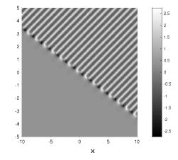
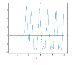
   Figure 3: Density plot of $\phi^{(1)}(x,t)$ and a snapshot of $\phi^{(1)}$ at t=0 ($\alpha=(1,1,1)$, $\nu=0.4$) .

Therefore, in the case $N=3$ we have only two types of kink solutions. To the best of our knowledge the wave front solutions (see Figure 3) represent a new class of exact solutions for integrable models.

4.1.2 Classification of rank $1$ kink solutions in the case where $N=4$

For $N=4$ equation (4) can be rewritten in the form

$$\begin{array}[]{l}2\phi^{(i)}_{t}=\phi^{(i+1)}_{xx}-\phi^{(i+3)}_{xx}+\phi^{(i)}_{x}(\phi^{(i+1)}_{x}-\phi^{(i+3)}_{x})+2e^{2\phi^{(i+1)}}-2e^{2\phi^{(i-1)}},\end{array}$$ (102)

where $\phi^{(i+4)}=\phi^{(i)}$ and $\sum_{i=1}^{4}\phi^{(i)}=0$. We classify its all possible rank $1$ kink solutions.

We first consider the case when $\mu=\mu^{\star}=\nu$ and the constant real vector

$${\mathbf{n}}_{0}=\alpha_{1}{\mathbf{e}}_{1}+\alpha_{2}{\mathbf{e}}_{2}+\alpha_{3}{\mathbf{e}}_{3}+\alpha_{4}{\mathbf{e}}_{4},$$

where $\alpha=(\alpha_{1},\alpha_{2},\alpha_{3},\alpha_{4}),\ \alpha_{3}=\alpha_{1}^{\star}\in{\mathbb{C}},\ \alpha_{2},\alpha_{4}\in{\mathbb{R}}$. In variables $\xi=(\nu-\nu^{-1})x$, $\zeta=(\nu+\nu^{-1})x$ and $\eta=(\nu^{-2}-\nu^{2})t$ we have

$$\Psi_{0}(x,t,\nu){\mathbf{e}}_{1}=e^{-\zeta{\rm i}+\eta}{\mathbf{e}}_{1};\quad\Psi_{0}(x,t,\nu){\mathbf{e}}_{2}=e^{-\xi-\eta}{\mathbf{e}}_{2};\quad\Psi_{0}(x,t,\nu){\mathbf{e}}_{3}=e^{\zeta{\rm i}+\eta}{\mathbf{e}}_{3};\quad\Psi_{0}(x,t,\nu){\mathbf{e}}_{4}=e^{\xi-\eta}{\mathbf{e}}_{4}.$$

There are four cases (excluding the trivial solutions) :

1. $\alpha_{2}$ and $\alpha_{4}$ are both non-zero real numbers, and $\alpha_{1}=\alpha_{3}=0$. We can take $\alpha_{4}=1$, then

   $${\mathbf{n}}=(e^{\xi-\eta}-\alpha_{2}e^{-\xi-\eta},e^{\xi-\eta}+\alpha_{2}e^{-\xi-\eta},e^{\xi-\eta}-\alpha_{2}e^{-\xi-\eta},e^{\xi-\eta}+\alpha_{2}e^{-\xi-\eta})^{\mbox{tr}}$$

   $$\quad=e^{\xi-\eta}(1-\alpha_{2}e^{-2\xi},1+\alpha_{2}e^{-2\xi},1-\alpha_{2}e^{-2\xi},1+\alpha_{2}e^{-2\xi})^{\mbox{tr}}.$$

   This leads to

   $$\tau_{j}=e^{2\xi-2\eta}\left((1-\alpha_{2}e^{-2\xi})^{2}(\nu^{2\{(j-1)\!\!\mod 4\}}+\nu^{2\{(j-3)\!\!\mod 4\}})\right.$$

   $$\qquad\left.+(1+\alpha_{2}e^{-2\xi})^{2}(\nu^{2\{(j-2)\!\!\mod 4\}}+\nu^{2\{j\!\!\mod 4\}})\right)/(\nu^{8}-1)$$

   $$\qquad=e^{2\xi-2\eta}\left(\frac{1+\alpha_{2}^{2}e^{-4\xi}}{\nu^{2}-1}-(-1)^{j}\frac{2\alpha_{2}e^{-2\xi}}{\nu^{2}+1}\right).$$

   Using (54), we obtain the solution

   $$\phi^{(j)}=\frac{1}{2}\ln\left(\frac{\tau_{j-1}\tau_{j+1}}{\tau_{j}^{2}}\right)=\ln\left|\frac{(1+\alpha_{2}^{2}e^{-4\xi})(\nu^{2}+1)+2\alpha_{2}e^{-2\xi}(-1)^{j}(\nu^{2}-1)}{(1+\alpha_{2}^{2}e^{-4\xi})(\nu^{2}+1)-2\alpha_{2}e^{-2\xi}(-1)^{j}(\nu^{2}-1)}\right|,$$

   which is independent of time $t$ (see left plot in Figure 4).

   

   

   Figure 4: Graph of $\phi^{(1)}(x,t)$ for kink solutions with $\nu=0.3$: on the left $\alpha=(0,1,0,1)$ and on the right $\alpha=(1,0,1,0)$

   This solution is of type (98).

2. $\alpha_{2}=\alpha_{4}=0,\alpha_{1}\alpha_{3}\neq 0$. Without the loss of generality, we take $\alpha_{1}=e^{{\rm i}\beta}=\alpha_{3}^{\star},$ where $\beta\in{\mathbb{R}}$ is a real constant. Then

   $${\mathbf{n}}=2e^{\eta}(\sin(\zeta-\beta),-\cos(\zeta-\beta),-\sin(\zeta-\beta),\cos(\zeta-\beta))^{\mbox{tr}}.$$

   Using (54), we obtain the solution

   $$\phi^{(j)}=\frac{1}{2}\ln\left(\frac{\tau_{j-1}\tau_{j+1}}{\tau_{j}^{2}}\right),$$

   $$\tau_{j}=\sin^{2}(\zeta-\beta)(\nu^{2\{(j-1)\!\!\mod 4\}}-\nu^{2\{(j-3)\!\!\mod 4\}})+\cos^{2}(\zeta-\beta)(\nu^{2\{j\!\!\mod 4\}}-\nu^{2\{(j-2)\!\!\mod 4\}})$$

   Here we get periodic solutions (see right plot in Figure 4). This is also a solution of type (98).

3. Only one of $\alpha_{2}$ and $\alpha_{4}$ is nonzero, and $\alpha_{1}=e^{{\rm i}\beta},\alpha_{3}=e^{-{\rm i}\beta}$, where $\beta\in{\mathbb{R}}$ is constant. Using Proposition 5, we are able to write down the solutions for $\phi^{(j)}$. Here we ignore the tedious formula and only show their plots, see first two density plots in Figure 5.

4. $\alpha_{1}\alpha_{2}\alpha_{3}\alpha_{4}\neq 0$. Let $\alpha_{1}=e^{{\rm i}\beta},\alpha_{3}=e^{-{\rm i}\beta}$ , where $\beta\in{\mathbb{R}}$ is constant. We take $\alpha_{2},\alpha_{4}\in{\mathbb{R}}$. The right plot in Figure 5 is its density plot.

   

   

   

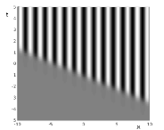
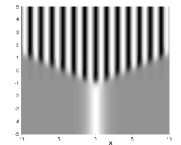
   Figure 5: Density plot of $\phi^{(1)}(x,t)$ for kink solutions with $\nu=0.7$ and $\alpha$ equals to $(1,1,1,0)$ for the left plot, $(1,0,1,1)$ for the middle plot and $(1,1,1,1)$ for the right plot.

For an even dimension, we also need to consider the case stated in Proposition 6. Let $\mu=\nu\exp(\frac{\pi{\rm i}}{4})$ and the constant vector

$${\mathbf{n}}_{0}=\alpha_{1}{\mathbf{e}}_{1}+\alpha_{2}{\mathbf{e}}_{2}+\alpha_{3}{\mathbf{e}}_{3}+\alpha_{4}{\mathbf{e}}_{4},$$

where $\alpha_{i}\in{\mathbb{C}}$. Notice that

$${\mathbf{n}}_{0}^{\star}=\alpha_{1}^{\star}{\mathbf{e}}_{3}+\alpha_{2}^{\star}{\mathbf{e}}_{2}+\alpha_{3}^{\star}{\mathbf{e}}_{1}+\alpha_{4}^{\star}{\mathbf{e}}_{4},\quad Q{\mathbf{e}}_{i}={\mathbf{e}}_{i+1}.$$

The requirement that ${\mathbf{n}}_{0}=Q{\mathbf{n}}_{0}^{\star}=\alpha_{1}^{\star}{\mathbf{e}}_{4}+\alpha_{2}^{\star}{\mathbf{e}}_{3}+\alpha_{3}^{\star}{\mathbf{e}}_{2}+\alpha_{4}^{\star}{\mathbf{e}}_{1}$ implies that $\alpha_{1}=\alpha_{4}^{\star}$ and $\alpha_{2}=\alpha_{3}^{\star}$.

In variables $\xi=\frac{\sqrt{2}}{2}(\nu-\nu^{-1})x$, $\zeta=\frac{\sqrt{2}}{2}(\nu+\nu^{-1})x$ and $\eta=(\nu^{-2}+\nu^{2})t$ we have

$$\Psi_{0}(x,t,\mu){\mathbf{e}}_{1}=e^{\xi-(\zeta+\eta){\rm i}}{\mathbf{e}}_{1};\quad\Psi_{0}(x,t,\mu){\mathbf{e}}_{2}=e^{-\xi-(\zeta-\eta){\rm i}}{\mathbf{e}}_{2};$$

$$\Psi_{0}(x,t,\mu){\mathbf{e}}_{3}=e^{-\xi+(\zeta-\eta){\rm i}}{\mathbf{e}}_{3};\quad\Psi_{0}(x,t,\mu){\mathbf{e}}_{4}=e^{\xi+(\zeta+\eta){\rm i}}{\mathbf{e}}_{4}.$$

There are three cases:

1. $\alpha_{1}=\alpha_{4}=0$. Without the loss of generality, we take $\alpha_{2}=e^{{\rm i}\beta}=\alpha_{3}^{\star}$, where $\beta\in{\mathbb{R}}$. Then

   $${\mathbf{n}}=e^{-\xi}\left(\begin{array}[]{c}(1+{\rm i})\left(\sin(\zeta-\eta-\beta)-\cos(\zeta-\eta-\beta)\right)\\ -2{\rm i}\sin(\zeta-\eta-\beta)\\ (-1+{\rm i})\left(\sin(\zeta-\eta-\beta)+\cos(\zeta-\eta-\beta)\right)\\ 2\cos(\zeta-\eta-\beta)\end{array}\right)$$

   Let $\theta=2(\zeta-\eta-\beta)$. Using (55) we get

   $$\tau_{1}=2{\rm i}e^{-2\xi}\left((1-\cos\theta)\nu^{6}+(1+\sin\theta)\nu^{4}+(1+\cos\theta)\nu^{2}+1-\sin\theta\right);$$

   $$\tau_{2}=-2e^{-2\xi}\left((1+\sin\theta)\nu^{6}+(1+\cos\theta)\nu^{4}+(1-\sin\theta)\nu^{2}+1-\cos\theta\right);$$

   $$\tau_{3}=-2{\rm i}e^{-2\xi}\left((1-\cos\theta)\nu^{2}+1+\sin\theta+(1+\cos\theta)\nu^{6}+(1-\sin\theta)\nu^{4}\right);$$

   $$\tau_{4}=2e^{-2\xi}\left((1+\sin\theta)\nu^{2}+1+\cos\theta+(1-\sin\theta)\nu^{6}+(1-\cos\theta)\nu^{4}\right).$$

   Hence we obtain periodic solutions. The left plot in Figure 6 is its density plot.

2. $\alpha_{2}=\alpha_{3}=0$. Without the loss of generality, we take $\alpha_{1}=e^{{\rm i}\beta}=\alpha_{4}^{\star}$, where $\beta\in{\mathbb{R}}$. In this case, we also get periodic solution similar to the above case. The middle plot in Figure 6 is its density plot.

3. $\alpha_{1}\alpha_{2}\alpha_{2}\alpha_{4}\neq 0$. Let $\alpha_{1}=e^{{\rm i}\beta}=\alpha_{4}^{\star}$ and $\alpha_{2}=\rho e^{{\rm i}\gamma}=\alpha_{3}^{\star},\rho\neq 0$, where $\beta,\gamma,\rho\in{\mathbb{R}}$. Here we ignore the tedious formula and only show their density plots, see the right plot of Figure 6.

   

   

   

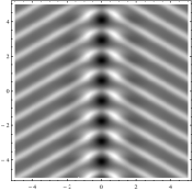
   Figure 6: Density plot of $\phi^{(1)}(x,t)$ for kink solutions with $\mu=\frac{3}{2}e^{\frac{\pi{\rm i}}{4}}$ and $\alpha$ equals to $(0,1,1,0)$ for the left plot, $(1,0,0,1)$ for the middle plot and $(1,1,1,1)$ for the right plot.

Therefore, in the case $N=4$ we have eight different rank $1$ kink solutions.

4.1.3 Classification of rank $1$ kink solutions for arbitrary dimensions

In this section, we classify all possible rank $1$ kink solutions for arbitrary dimension $N$. We have already explored how the solutions for lower dimensions $N=3,4$. There is a difference between the dimension $N$ being even or odd.

For arbitrary $N$, according to Proposition 5, our kink solution depends only on ${\mathbf{n}}_{0}\in{\mathbb{R}}^{N}$ and $\nu\in{\mathbb{R}},\nu\notin\{\pm 1,0\}$. We can decompose $\mathbb{R}^{N}$ as a direct sum of invariant subspaces of $\Delta$ as follows:

$$N=2m-1,\quad\mathbb{R}^{N}=E^{1}_{0}\bigoplus_{p=1}^{m-1}E^{2}_{p};$$

$$N=2m,\qquad\mathbb{R}^{N}=E^{1}_{0}\bigoplus E^{1}_{m}\bigoplus_{p=1}^{m-1}E^{2}_{p},$$

where

$$E^{1}_{0}=\mbox{span}_{\mathbb{R}}({\bf e}_{N}),\ E^{1}_{m}=\mbox{span}_{\mathbb{R}}({\bf e}_{m}),\ E^{2}_{p}=\mbox{span}_{\mathbb{R}}(\mbox{Re}\,({\bf e}_{p}),\mbox{Im}\,({\bf e}_{p})).$$

We define “elementary waves” as solutions corresponding to the case where ${\mathbf{n}}_{0}$ is simply a combination of two eigenvectors. When $N=2m$, there are $m$ elementary waves: one pair of real eigenvalues and $m-1$ pairs of complex conjugate eigenvalues. When $N=2m-1$, there are $m-1$ elementary wave solutions since there is only one real eigenvalue, which leads to trivial solutions and we exclude it. The other solutions can be built from these elementary wave solutions together with trivial solutions.

We are able to write down the elementary wave solutions for arbitrary $N$. To do so, we make use the following identity: For fixed $p\in{\mathbb{N}}$ and $\omega^{N}=1$, by direct computation we have

$$\sum_{l=1}^{N}\omega^{pl}\mu^{2\{(j-l)\!\!\mod N\}}=\frac{\mu^{2N}-1}{\mu^{2}\omega^{-p}-1}\omega^{pj},\quad\mu\in{\mathbb{C}}.$$ (104)

Theorem 1.

For any given nonzero constants $\beta,\nu\in{\mathbb{R}}$, $N\in{\mathbb{N}},\ \nu^{2}\neq 1,\ N>2$ and $p\in\{1,\cdots\lfloor\frac{N-1}{2}\rfloor\}$, system (4) has elementary periodic wave solution of rank $1$ given by

$$\phi^{(j)}=\frac{1}{2}\ln\frac{\tau_{j-1}\tau_{j+1}}{\tau_{j}^{2}},\qquad\tau_{j}=\frac{\nu^{2}\cos(2b-\frac{4p(j+1)\pi}{N})-\cos(2b-\frac{4pj\pi}{N})}{|\nu^{2}\omega^{2p}-1|^{2}}+\frac{1}{\nu^{2}-1},$$

where

$$b=(\nu+\frac{1}{\nu})\sin(\frac{2p\pi}{N})x+(\nu^{2}+\frac{1}{\nu^{2}})\sin(\frac{4p\pi}{N})t-\beta.$$ (105)

For even $N=2m$, there is also a time independent rank $1$ elementary kink solution of the form

$$\phi^{(j)}=\ln\left|\frac{(\beta^{2}+e^{-4\xi})(\nu^{2}+1)+2\beta e^{-2\xi}(-1)^{j}(\nu^{2}-1)}{(\beta^{2}+e^{-4\xi})(\nu^{2}+1)-2\beta e^{-2\xi}(-1)^{j}(\nu^{2}-1)}\right|,\qquad\xi=(\nu-\frac{1}{\nu})x.$$

Proof.

Let us take ${\mathbf{n}}_{0}=e^{{\rm i}\beta}{\mathbf{e}}_{p}+e^{-{\rm i}\beta}{\mathbf{e}}_{N-p}$ then the $k$-th component of the vector ${\mathbf{n}}=\Psi_{0}(x,t,\nu){\mathbf{n}}_{0}$ can be written as follows:

$${\mathbf{n}}_{k}=e^{(\frac{\nu}{\omega^{p}}-\frac{\omega^{p}}{\nu})x+(\frac{\nu^{2}}{\omega^{2p}}-\frac{\omega^{2p}}{\nu^{2}})t+\beta{\rm i}}({\bf e}_{p})_{k}+e^{(\nu\omega^{p}-\frac{1}{\omega^{p}\nu})x+(\nu^{2}\omega^{2p}-\frac{1}{\omega^{2p}\nu^{2}})t-\beta{\rm i}}({\bf e}_{N-p})_{k}=e^{a}\left(e^{-b{\rm i}}\omega^{kp}+e^{b{\rm i}}\omega^{-kp}\right),$$

where

$$a=(\nu-\frac{1}{\nu})\cos(\frac{2p\pi}{N})x+(\nu^{2}-\frac{1}{\nu^{2}})\cos(\frac{4p\pi}{N})t$$

and $b$ is defined by (105). It follows from (54) that

$$\tau_{j}=\frac{1}{\nu^{2N}-1}e^{2a}\sum_{k=1}^{N}\left(\left(e^{-b{\rm i}}\omega^{kp}+e^{b{\rm i}}\omega^{-kp}\right)^{2}\right)\nu^{2\{(j-k)\mod N\}}$$

$$\qquad=e^{2a}\left(e^{-2b{\rm i}}\frac{\omega^{2pj}}{\nu^{2}\omega^{-2p}-1}+e^{2b{\rm i}}\frac{\omega^{-2pj}}{\nu^{2}\omega^{2p}-1}+\frac{2}{\nu^{2}-1}\right)$$

$$\qquad=2e^{2a}\left(\frac{\nu^{2}\cos(2b-\frac{4p(j+1)\pi}{N})-\cos(2b-\frac{4pj\pi}{N})}{|\nu^{2}\omega^{2p}-1|^{2}}+\frac{1}{\nu^{2}-1}\right),$$

which leads to the periodic solutions for $\phi^{(j)}$ given in the statement.

Similarly, in the case $N=2m$, we compute the solution corresponding to ${\mathbf{n}}_{0}={\mathbf{e}}_{m}+\beta{\mathbf{e}}_{2m}$. Now we have

$${\mathbf{n}}_{k}=\beta e^{(\nu-\frac{1}{\nu})x+(\nu^{2}-\frac{1}{\nu^{2}})t}+(-1)^{k}e^{(-\nu+\frac{1}{\nu})x+(\nu^{2}-\frac{1}{\nu^{2}})t}=e^{(\nu-\frac{1}{\nu})x+(\nu^{2}-\frac{1}{\nu^{2}})t}\left(\beta+(-1)^{k}e^{-2(\nu-\frac{1}{\nu})x})\right),$$

where $k=1,\cdots N=2m$. This leads to

$$\tau_{j}=e^{2(\nu-\frac{1}{\nu})x+2(\nu^{2}-\frac{1}{\nu^{2}})t}\left(\frac{\beta^{2}+e^{-4(\nu-\frac{1}{\nu})x}}{\nu^{2}-1}+(-1)^{j+1}\frac{2\beta e^{-2(\nu-\frac{1}{\nu})x}}{\nu^{2}+1}\right),$$

which gives us the solutions $\phi^{(j)}$ independent of time $t$ given in the statement. ∎

When $N=2m$, according to Proposition 6, to get kink solutions we take $\mu=\nu e^{\frac{\pi{\rm i}}{2m}}$ and ${\mathbf{n}}_{0}=Q{\mathbf{n}}_{0}^{\star}$. It follows from (99) there are also $m$ elementary waves. Similar to Theorem 1, we explicitly derive the elementary solutions in this case.

Theorem 2.

Let $N=2m$, where the integer $m\geq 2$. For any given nonzero constants $\beta,\nu\in{\mathbb{R}}$ and $p\in\{1,\cdots m\}$, system (4) has elementary periodic wave solution of rank $1$ given by

$$\phi^{(j)}=\frac{1}{2}\ln\frac{\tau_{j-1}\tau_{j+1}}{\tau_{j}^{2}},\qquad\tau_{j}=\frac{\nu^{2}\cos(2b-\frac{(2p-1)(j+1)\pi}{m})-\cos(2b-\frac{(2p-1)j\pi}{m})}{|\nu^{2}\omega^{2p-1}-1|^{2}}+\frac{1}{\nu^{2}-1},$$

where

$$b=(\nu+\frac{1}{\nu})\sin(\frac{(2p-1)\pi}{2m})x+(\nu^{2}+\frac{1}{\nu^{2}})\sin(\frac{(2p-1)\pi}{m})t-\beta.$$ (106)

Proof.

For $\mu=\nu\exp(\frac{\pi{\rm i}}{2m})$, we take ${\mathbf{n}}_{0}=e^{{\rm i}\beta}{\mathbf{e}}_{p}+e^{-{\rm i}\beta}{\mathbf{e}}_{2m-p+1}$ following from (99) and then the $k$-th component of the vector ${\mathbf{n}}=\Psi_{0}(x,t,\nu){\mathbf{n}}_{0}$ can be written as follows:

$${\mathbf{n}}_{k}=e^{(\frac{\nu}{\omega^{p-\frac{1}{2}}}-\frac{\omega^{p-\frac{1}{2}}}{\nu})x+(\frac{\nu^{2}}{\omega^{2p-1}}-\frac{\omega^{2p-1}}{\nu^{2}})t+\beta{\rm i}}({\bf e}_{p})_{k}+e^{(\nu\omega^{p-\frac{1}{2}}-\frac{\omega^{\frac{1}{2}-p}}{\nu})x+(\nu^{2}\omega^{2p-1}-\frac{1}{\omega^{2p-1}\nu^{2}})t-\beta{\rm i}}({\bf e}_{2m-p+1})_{k}$$

$$=e^{a}\left(e^{-b{\rm i}}\omega^{kp}+e^{b{\rm i}}\omega^{-k(p-1)}\right),$$

where

$$a=(\nu-\frac{1}{\nu})\cos(\frac{(2p-1)\pi}{2m})x+(\nu^{2}-\frac{1}{\nu^{2}})\cos(\frac{(2p-1)\pi}{m})t$$

and $b$ is defined by (106). It follows from (55) that

$$\tau_{j}=\frac{1}{\nu^{2N}-1}e^{2a}\sum_{k=1}^{N}\left(\left(e^{-b{\rm i}}\omega^{kp}+e^{b{\rm i}}\omega^{-k(p-1)}\right)^{2}\right)\mu^{2\{(j-k)\mod N\}}$$

$$\qquad=e^{2a}\left(e^{-2b{\rm i}}\frac{\omega^{2pj}}{\mu^{2}\omega^{-2p}-1}+e^{2b{\rm i}}\frac{\omega^{(2-2p)j}}{\mu^{2}\omega^{2p-2}-1}+\frac{2\omega^{j}}{\mu^{2}\omega^{-1}-1}\right)$$

$$\qquad=2e^{2a}\omega^{j}\left(\frac{\nu^{2}\cos(2b-\frac{(2p-1)(j+1)\pi}{m})-\cos(2b-\frac{(2p-1)j\pi}{m})}{|\nu^{2}\omega^{2p-1}-1|^{2}}+\frac{1}{\nu^{2}-1}\right),$$

which leads to the periodic solutions for $\phi^{(j)}$ given in the statement. ∎

Elementary rank $1$ kink solutions correspond to two dimensional $\Delta$–invariant subspaces of ${\mathbb{R}}^{N}$. Other rank 1 solutions correspond to invariant subspaces of dimension $3,4,\ldots,N$. The number of all possible $\Delta$–invariant subspaces gives us the number of all rank 1 solutions.

Theorem 3.

Equation (4) with odd $N=2m-1$ has $2^{m}-2$ different rank $1$ kink solutions. In the case of even $N=2m$ it has $3\cdot 2^{m}-4$ different rank $1$ kink solutions.

Proof.

When $N=2m-1$, there are $m-1$ elementary solutions from ${\mathbf{n}}_{0}\in E^{2}_{p}$ for each $p=1,2,\cdots,m-1$, and one constant solution from ${\mathbf{n}}_{0}\in E^{1}_{0}$. We can build up other solutions by taking any combination of them. For example, there are $C_{m}^{2}=\frac{m(m-1)}{2}$ different solutions if we take any two combinations. Thus, the total number of different rank $1$ kink solutions is

$$m-1+\sum_{k=2}^{m}C_{m}^{k}=2^{m}-2.$$

When $N=2m$, when $\mu=\nu\in{\mathbb{R}}$ there are $m-1$ elementary solutions from ${\mathbf{n}}_{0}\in E^{2}_{p}$ for each $p=1,2,\cdots,m-1$, one elementary solution from ${\mathbf{n}}_{0}\in E^{1}_{0}\bigoplus E^{1}_{m}$ and two constant solutions from ${\mathbf{n}}_{0}\in E^{1}_{0}$ or ${\mathbf{n}}_{0}\in E^{1}_{m}$. we can build up other solutions by taking any combinations of $m-1$ elementary solutions alone or together with either one real or both real eigenvectors. Thus, the total number of different rank $1$ kink solutions in this case is

$$1+4\sum_{k=1}^{m}C_{m-1}^{k}=4(2^{m-1}-1)+1=2^{m+1}-3.$$

When $N=2m$, when $\mu=\nu e^{\frac{\pi{\rm i}}{2m}},\nu\in{\mathbb{R}}$ there are also $m$ elementary solutions. In this case the total number of different rank $1$ kink solutions is

$$\sum_{k=1}^{m}C_{m}^{k}=2^{m}-1.$$

Hence when $N=2m$, the total number of different rank $1$ kink solutions is $3\cdot 2^{m}-4$. Thus we complete the proof. ∎

Notice that the statement is consistent with the concrete results for $N=3$ and $N=4$. We plot some density plots of $\phi^{(1)}$ and snapshots for $N=5$ when $\nu=0.4$ and $\alpha$ are chosen as stated in Figures 7 and 8.

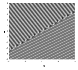
Figure 7: Density plot of $\phi^{(1)}(x,t)$ and a snapshot of $\phi^{(1)}$ at t=0 ($\alpha=(1,1,1,1,0)$, $\nu=0.4$) .

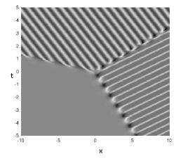
Figure 8: Density plot of $\phi^{(1)}(x,t)$ and a snapshot of $\phi^{(1)}$ at t=0.7 ($\alpha=(1,1,1,1,1)$, $\nu=0.4$) .

4.1.4 Tropicalisation and wave front trajectories

In the general case of rank 1 “kink” solutions the trajectories of the wave fronts can be understood geometrically. According Proposition 5 the $(x,t)$ dependence of the solution is determined by the vector ${\mathbf{n}}$ which can be presented in the form

$${\mathbf{n}}=\sum_{k=1}^{N}e^{\Theta_{k}(x,t)}{\mathbf{e}}_{k},$$

where

$$\Theta_{k}(x,t)=(\nu\omega^{-k}-\nu^{-1}\omega^{k})x+(\nu^{2}\omega^{-2k}-\nu^{-2}\omega^{2k})t+\log\alpha_{k}.$$

The imaginary part $\Theta_{k}^{\rm Im}(x,t)$ is responsible for oscillations of the solution, while the real part

$$\Theta_{k}^{\rm Re}(x,t)=(\nu-\nu^{-1})\cos(\frac{2\pi k}{N})x+(\nu^{2}-\nu^{-2})\cos(\frac{4\pi k}{N})t+\log|\alpha_{k}|$$

tells us which term in the sum is dominant at a given point $(x,t)$. In a region where only one term in the sum is dominant, and thus we can ignore other terms, the solution is close to the trivial (zero) solution. In regions where two terms have the same real exponent ($\Theta_{k}^{\rm Re}(x,t)=\Theta_{-k}^{\rm Re}(x,t)$) we observe elementary waves. The boundaries of these regions correspond to the wave fronts. Thus the wave fronts can be described as follows: We consider a set of linear functions $\Theta_{k}^{\rm Re}(x,t),\ k=1,\ldots,N$ and define a continuous piecewise linear function

$$\Theta(x,t)=\,\mbox{max}(\Theta_{1}^{\rm Re}(x,t),\cdots,\Theta_{N}^{\rm Re}(x,t)).$$ (107)

The locus where the function $\Theta(x,t)$ is not smooth corresponds to the wave fronts. To compare the numerical result for wave fronts with the locus described above one can compare Figures 8 and 9.

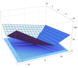
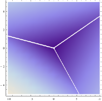
Figure 9: Density and 3-d plots for $\Theta(x,t)$, $N=5$, $\alpha=(1,1,1,1,1)$, $\nu=0.4$ (compare with Figure 8).

This construction is similar to tropicalisation and soliton graphs proposed by Kodama and Williams for the case of KP solitons [12], although there is a slight difference, since we do not use rescaling in our definition and keep the logarithmic term $\log|\alpha_{k}|$, which disappears in the scaling limit.

4.2 Classification of rank $1$ breather solutions for arbitrary dimensions

In this section, we classify all possible rank $1$ breather solutions for arbitrary dimension $N$. According to Proposition 9, our soliton solution depends only on ${\mathbf{n}}_{0}\in{\mathbb{C}}^{N}$, $\mu\in{\mathbb{C}}$ and $|\mu|\notin\{0,1\}$. In a similar manner to the case for kinks, a natural way to classify possible solutions in terms of ${\mathbf{n}}_{0}$ is to first consider eigenvectors and eigenvalues of the constant matrix $\Delta$. We decompose ${\mathbb{C}}^{N}$ as a direct sum of invariant subspaces of $\Delta$ as follows:

$$\mathbb{C}^{N}=\bigoplus_{p=1}^{N}E^{1}_{p},\qquad E^{1}_{p}=\mbox{span}_{\mathbb{C}}({\bf e}_{p}).$$

The vector ${\mathbf{n}}_{0}$ in this basis

$${\mathbf{n}}_{0}=\sum_{p=1}^{N}\alpha_{p}{\mathbf{e}}_{p},\qquad\alpha_{p}\in{\mathbb{C}}$$ (108)

is given by a matrix $\alpha=(\alpha_{1},\ldots,\alpha_{N})$. We immediately get the following result:

Proposition 12.

For a constant complex vector ${\mathbf{n}}_{0}$ in the form of (108), if there is only one $\alpha_{p}$ is nonzero, then solutions for (4) are trivial, that is, $\phi^{(i)}=0$.

Proof.

It follows from (104) that

$$\frac{1}{\mu^{2N}-1}\sum_{l=1}^{N}\omega^{2pl}\mu^{2\{(i-l)\!\!\!\mod N\}}=\frac{\omega^{2p(i+1)}}{\mu^{2}-\omega^{2p}};\qquad\frac{1}{|\mu|^{2N}-1}\sum_{l=1}^{N}|\mu|^{2\{(i-l)\!\!\!\mod N\}}=\frac{1}{|\mu|^{2}-1}.$$

Thus we can compute $\tau_{i}$ in (69) as follows:

$$\tau_{i}=|\alpha_{p}|^{4}|e^{(\frac{\mu}{\omega^{p}}-\frac{\omega^{p}}{\mu})x+(\frac{\mu^{2}}{\omega^{2p}}-\frac{\omega^{2p}}{\mu^{2}})t}|^{4}\left(\frac{1}{(|\mu|^{2}-1)^{2}}-\frac{1}{|\mu^{2}-\omega^{2p}|^{2}}\right),$$

which is independent of $i$. According to Proposition 9, we get solutions $\phi^{(i)}=0$ as stated. ∎

We now consider the case when there are only two nonzero components, say $\alpha_{p}$ and $\alpha_{q}$ among all $\alpha_{i},i=1,\cdots,N$, that is,

$${\mathbf{n}}_{0}=\alpha_{p}{\mathbf{e}}_{p}+\alpha_{q}{\mathbf{e}}_{q},\qquad\alpha_{p}\alpha_{q}\neq 0,\qquad q>p.$$ (109)

It follows that the $k$-component of vector ${\mathbf{n}}$ is

$$n_{k}=\alpha_{p}e^{(\frac{\mu}{\omega^{p}}-\frac{\omega^{p}}{\mu})x+(\frac{\mu^{2}}{\omega^{2p}}-\frac{\omega^{2p}}{\mu^{2}})t}\omega^{kp}+\alpha_{q}e^{(\frac{\mu}{\omega^{q}}-\frac{\omega^{q}}{\mu})x+(\frac{\mu^{2}}{\omega^{2q}}-\frac{\omega^{2q}}{\mu^{2}})t}\omega^{kq}=A(\omega^{kp}+\gamma\omega^{kq}),$$

where we introduce notations for $A,\gamma\in{\mathbb{C}}$ to shorten the expressions of $\sigma(j)$ and $\rho(j)$ defined by (70). We have

$$\sigma(j)=A^{2}(\frac{\omega^{2p(j+1)}}{\mu^{2}-\omega^{2p}}+2\gamma\frac{\omega^{(p+q)(j+1)}}{\mu^{2}-\omega^{p+q}}+\gamma^{2}\frac{\omega^{2q(j+1)}}{\mu^{2}-\omega^{2q}});$$

$$\rho(j)=|A|^{2}\left((1+|\gamma|^{2})\frac{1}{|\mu|^{2}-1}+\gamma^{*}\frac{\omega^{(p-q)(j+1)}}{|\mu|^{2}-\omega^{p-q}}+\gamma\frac{\omega^{(q-p)(j+1)}}{|\mu|^{2}-\omega^{q-p}}\right).$$

According to Proposition 9, the breather solutions depend on $\gamma$ and $\mu$ since $A$ is cancelled when we compute the solutions. Let $\mu=|\mu|e^{i\delta}$. The breather trajectory is determined by the condition $|\gamma|=1$, where

$$|\gamma|=|\frac{\alpha_{q}}{\alpha_{p}}||e^{(\frac{\mu}{\omega^{q}}-\frac{\omega^{q}}{\mu}-\frac{\mu}{\omega^{p}}+\frac{\omega^{p}}{\mu})x+(\frac{\mu^{2}}{\omega^{2q}}-\frac{\omega^{2q}}{\mu^{2}}-\frac{\mu^{2}}{\omega^{2p}}+\frac{\omega^{2p}}{\mu^{2}})t}|$$

$$\qquad=e^{(|\mu|-\frac{1}{|\mu|})(\cos(\delta-\frac{2\pi q}{N})-\cos(\delta-\frac{2\pi p}{N}))x+(|\mu|^{2}-\frac{1}{|\mu|^{2}})(\cos(2\delta-\frac{4\pi q}{N})-\cos(2\delta-\frac{4\pi p}{N}))t+\ln|\frac{\alpha_{q}}{\alpha_{p}}|}$$

$$\qquad=e^{2(|\mu|-\frac{1}{|\mu|})\sin(\delta-\frac{(p+q)\pi}{N})\sin\frac{(q-p)\pi}{N}(x-v_{pq}t-x_{pq}^{0})}.$$

It reflects the balance between the exponents. Thus the speed of the breather is given by

$$v_{pq}=-4\left(\frac{1}{|\mu|}+|\mu|\right)\cos\left(\delta-\frac{\pi(p+q)}{N}\right)\cos\left(\frac{\pi(q-p)}{N}\right)$$

and it is shifted to the right along the $x$-axis by

$$x_{pq}^{0}=\frac{\ln|\frac{\alpha_{p}}{\alpha_{q}}|}{2(|\mu|-\frac{1}{|\mu|})\sin(\delta-\frac{(p+q)\pi}{N})\sin\frac{(q-p)\pi}{N}}.$$

It is localised in $x$ and of size $L_{pq}$

$$L^{-1}_{pq}=2(|\mu|-|\mu|^{-1})\sin(\delta-\frac{(p+q)\pi}{N})\sin\frac{(q-p)\pi}{N}.$$

The rank $1$ breather solutions can be obtained in the following way:

• There are $C_{N}^{2}$ possible choices of two dimensional $\Delta$–invariant subspaces in ${\mathbb{C}}^{N}$ and therefore there are $C_{N}^{2}$ elementary breathers.

• Solutions corresponding to three dimensional invariant subspaces, i.e.

  $${\mathbf{n}}_{0}=\alpha_{p}{\mathbf{e}}_{p}+\alpha_{q}{\mathbf{e}}_{q}+\alpha_{r}{\mathbf{e}}_{r},\ \alpha_{p}\alpha_{q}\alpha_{r}\neq 0$$

  represent decays or fusions of breathers (“Y” shape), and there are $C_{N}^{3}$ such solutions.

• Solutions corresponding to four dimensional invariant subspaces, i.e.

  $${\mathbf{n}}_{0}=\alpha_{p}{\mathbf{e}}_{p}+\alpha_{q}{\mathbf{e}}_{q}+\alpha_{r}{\mathbf{e}}_{r}+\alpha_{s}{\mathbf{e}}_{s},\ \alpha_{p}\alpha_{q}\alpha_{r}\alpha_{s}\neq 0$$

  represent solutions combining 2 “Y” shapes (“2Y” shape solutions). There are $C_{N}^{4}$ such solutions, etc.

Examples of “Y”, “2Y” and “3Y” configurations in the case $N=5$ are presented in Figure 10.

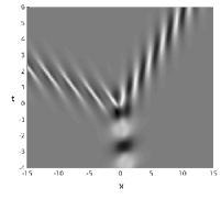
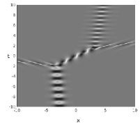
Figure 10: Density plots of $\phi^{(1)}(x,t)$ for breather solutions $N=5$ with $\mu=0.7+0.15{\rm i},\ \alpha=(1,0,1,0,1)$, and $\mu=0.5+0.15{\rm i},\ \alpha=(1,0.01,1,0,0.0001)$, and $\mu=0.3+0.15{\rm i},\ \alpha=(0.01,1,10,10{\rm i},0.1)$ respectively.

The total number of possible distinct configurations for a breather solution given in Proposition 9 is

$$\sum_{k=2}^{N}C_{N}^{k}=2^{N}-N-1.$$

The type of the breather solution depends on the choice of the matrix $\alpha=(\alpha_{1},\ldots,\alpha_{N})$. The explicit expression for the solution is given in Proposition 9 and it is quite complicated, but the method of tropicalisation, which we used in Section 4.1.4, enables us to give a simple description of the soliton graph. We explore the observation that the vector

$${\mathbf{n}}=\sum_{k=1}^{N}e^{\Theta_{p}(x,t)}{\mathbf{e}}_{p},$$

where

$$\Theta_{p}(x,t)=(\frac{\mu}{\omega^{p}}-\frac{\omega^{p}}{\mu})x+(\frac{\mu^{2}}{\omega^{2p}}-\frac{\omega^{2p}}{\mu^{2}})t+\log\alpha_{p},\quad\mu=|\mu|e^{\delta}$$

completely determines the $(x,t)$ dependence of the solution. In the regions where only one term is dominant the solution is exponentially small. We can define the tropical graph of the breather as a locus where two or more terms are in balance. More precisely, let us consider the real part of $\Theta_{p}(x,t)$, that is,

$$\Theta_{p}^{\rm Re}(x,t)=(|\mu|-|\mu|^{-1})\cos(\delta-\frac{2\pi p}{N})x+(|\mu|^{2}-|\mu|^{-2})\cos(2\delta-\frac{4\pi p}{N})t+\log|\alpha_{p}|$$

and a piecewise linear continuous function of variables $(x,t)$:

$$\Theta(x,t)=\,\mbox{max}_{p}\Theta_{p}^{\rm Re}(x,t).$$

Definition 1.

For rank one breather solutions the tropical soliton graph is defined as a locus of points where the function $\Theta(x,t)$ is not smooth.

In order to visualise the tropical plot we present the density plot for the piecewise constant function $\partial_{x}\Theta(x,t)$. In Figure 11 we show the plots corresponding to solutions plotted in Figure 10.

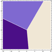
Figure 11: Tropical plots of $\phi^{(1)}(x,t)$ for breather solutions $N=5$ with parameters $\mu$ and $\alpha$ corresponding to plots on Figure 10.

This definition does not reflect the fact that we are dealing with a system of equations and thus the graphs corresponding to the variables $\phi^{(i)}(x,t),\ i=1,\ldots,N$ are slightly different (they may depend on the index $i$). It can be considered as a first approximation which does capture well the trajectories of the solitons (breathers).

The general approach to visualisation of rank $r$ solutions is similar to the case of rank one. We use the fact that a rank $r$ solution is a function of the point

$${\mathbf{n}}(x,t)=\exp((\mu\Delta^{-1}-\mu^{-1}\Delta)x-(\mu^{-2}\Delta^{2}-\mu^{2}\Delta^{-2})t){\mathbf{n}}_{0}$$

on the Grassmannian ${\rm Gr}(r,N)$, where ${\mathbf{n}}(x,t)$ is a $N\times r$ full rank matrix (as it follows from Proposition 10). In the basis ${\mathbf{e}}_{k}$ (96) the matrix ${\mathbf{n}}(x,t)$ can be represented as

$${\mathbf{n}}(x,t)=({\mathbf{e}}_{1},\ldots,{\mathbf{e}}_{N}){\alpha}^{\mbox{tr}}(x,t),$$

where $\alpha(x,t)$ is $r\times N$ matrix of full rank and

$$\left(\alpha(x,t)\right)_{pq}=\alpha^{(0)}_{pq}\exp((\mu\omega^{-q}-\mu^{-1}\omega^{q})x-(\mu^{-2}\omega^{2q}-\mu^{2}\omega^{-2q})t),\qquad 1\leq p\leq r,\ 1\leq q\leq N.$$

Let

$$I=\{i_{1}<i_{2}<\ldots<i_{k}\}\subset[1,\ldots,N]$$

and let $\Delta_{I}(x,t)$ denote the minor of $\alpha(x,t)$ with columns $i_{1},\ldots,i_{k}$ (a Plücker coordinate on the Grassmannian ${\rm Gr}(k,N)$). Let us define $\Theta_{I}(x,t)=\log|\Delta_{I}(x,t)|$ if $\Delta_{I}(x,t)\neq 0$ and for such $I$ that $\Delta_{I}(x,t)=0$ we set $\Theta_{I}(x,t)=-\infty$. The function $\Theta_{I}(x,t)$ is a linear function of the coordinates $(x,t)$. If there is only one nonzero minor $\Delta_{I}(x,t)$, then it is easy to show that the corresponding solution is $\phi^{(i)}(x,t)=0,\ i=1,\ldots,N$ (similar to Proposition 12). The solution is concentrated near the points where two or more Plücker coordinates are in balance and we can give the following definition of the tropical soliton graph in the case of rank $r$ breather solutions.

Definition 2.

For rank $r$ breather solutions the tropical soliton graph is defined as a locus of points where the function $\Theta(x,t)=\,\mbox{max}_{I}\Theta_{I}(x,t)$ is not smooth.

Using the definition, we plot the tropical soliton graph for

$$N=5,\qquad\mu=0.57+0.2{\rm i},\qquad\alpha=\left(\begin{array}[]{rrrrr}1&10&10^{4}&10^{3}&1\\ 10^{6}&1&10^{6}&10^{4}&99.9\end{array}\right)$$

and compare it to the actual density plot for $\phi^{(3)}(x,t)$ in the following graph:

Figure 12: Tropical and density plots of $\phi^{(3)}(x,t)$ for rank 2 breather solutions $N=5$

Although the above definition of a tropical soliton graph is not perfect (it does not reflect the dependence of the graph on the index $i$ for different components $\phi^{(i)}(x,t)$), it reflects well the picture of the breather interactions. It also opens a path to classification of possible configurations in the multi-soliton solutions of arbitrary rank.

5 Conclusion

In this paper we developed the dressing method for the two dimensional Volterra system (4). We have constructed two types of exact solutions to the system. The first type is rather unusual. It represents propagation of the wave fronts. Up to the best of our knowledge it is a new class of solutions in integrable models. The second type resembles breathers in the sine-Gordon equation. Nonlinear wave (“kink”) solutions are parametrised by a real parameter $\nu$ and a point on a real Grassmannian ${\rm Gr}_{\mathbb{R}}(k,N)$. In the case of breathers the parameter $\mu$ and Grassmannian ${\rm Gr}_{\mathbb{C}}(k,N)$ are complex. The integer $k$ is the rank of the solution. We have studied in detail the properties and configurations of rank 1 solutions, where the Grassmannians are real and complex projective spaces respectively. Classification of rank $k$ solutions can be linked with the classification of $\Delta$–invariant Schubert decompositions of the Grassmannians, where $\Delta$ is the cyclic shift matrix from the Lax representation of the two dimensional Volterra system (4).

In this paper we have not yet developed a classification of higher rank solutions, but we claim that their properties are quite different from the solutions of rank one. For example the nonlinear wave (“kink”) solutions of rank 2 may represent a nonlinear interference of waves (see Figure 1, right) which is impossible in the case of rank one solutions. In the case $N=4$ we have listed in Section 4.1.2 and presented all possible rank 1 kink solutions. Here we present density plots for two kink solutions of rank 2 when $N=4$ in Figure 13 and some snapshots in Figure 14, which does not resemble any rank 1 solution.

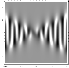
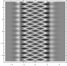
Figure 13: Density plot of $\phi^{(1)}(x,t)$ for a kink solution of rank $2$ when $N=4$: $\nu=0.8,{\mathbf{n}}_{0}=({\rm i}{\mathbf{e}}_{1}-2{\mathbf{e}}_{2}-{\rm i}{\mathbf{e}}_{3}+{\mathbf{e}}_{4},\ 2{\mathbf{e}}_{1}+{\mathbf{e}}_{2}+2{\mathbf{e}}_{3}+{\mathbf{e}}_{4})$ for the left plot and $\mu=2e^{\frac{\pi{\rm i}}{4}},{\mathbf{n}}_{0}=({\mathbf{e}}_{1}+(1+100{\rm i}){\mathbf{e}}_{2}+{\mathbf{e}}_{3}+(1-100{\rm i}){\mathbf{e}}_{4},\ 10{\rm i}{\mathbf{e}}_{1}+5{\rm i}{\mathbf{e}}_{2}-10{\rm i}{\mathbf{e}}_{3}-5{\rm i}{\mathbf{e}}_{4})$ for the right plot.

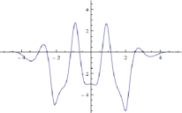
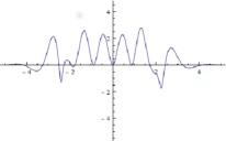
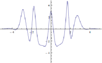
Figure 14: Snapshots of $\phi^{(1)}(x,t)$ for rank $2$ kink solution on the right plot in Figure 13: $t=0.0945$ for the left plot, $t=-0.09075$ for the middle plot and $t=-0.276$ for the right plot.

Breather solutions of rank 1 do not have closed loops, but in rank 2 loops exist (see Figure 2).

To study the structure and classify higher rank wave front and breather solutions as well as multi-soliton solutions (with a finite number of orbits of the poles in the dressing matrix $\Phi(\lambda)$) we need to develop further methods similar to ones proposed by Kodama et al. for the KP equation [10, 11, 12]. There is also an interesting and as yet unsolved problem to find solutions of (4) which approximate for large $N$ the solutions of the KP equation.

References

- [1] V.E. Zakharov and A.B. Shabat. Integration of nonlinear equations of mathematical physics by the method of inverse scattering. II. Functional Analysis and Its Applications, 13(3):166–174, 1979.
- [2] V. E. Zakharov and A. V. Mikhailov. Relativistically invariant two-dimensional models of field theory which are integrable by means of the inverse scattering problem method. Zh. Èksper. Teoret. Fiz., 74(6):1953–1973, 1978.
- [3] V. Bargmann. On the connection between phase shifts and scattering potential. Rev. Mod. Phys., 21:488–493, Jul 1949.
- [4] Clifford S. Gardner, John M. Greene, Martin D. Kruskal, and Robert M. Miura. Method for solving the korteweg-devries equation. Phys. Rev. Lett., 19:1095–1097, Nov 1967.
- [5] P.D. Lax. Integrals of nonlinear equations of evolution and solitary waves. Communications on Pure and Applied Mathematics, 21:467–490, 1968.
- [6] A.V. Mikhailov. Integrability of a two-dimensional generalization of the Toda chain. JETP Lett., 30(7):414–418, 1979.
- [7] A.V. Mikhailov. The reduction problem and the inverse scattering method. Phys. D, 3(1& 2):73–117, 1981.
- [8] B. B. Kadomtsev and V. I. Petviashvili. On the stability of solitary waves in weakly dispersive media. Sov. Phys. Dokl., 15:539–541, 1970.
- [9] M. Sato and Y. Sato. Soliton equations as dynamical systems on infinite dimensional Grassman manifolds. In Lect. Notes in Appl. Anal., volume 5, pages 259–271. 1982.
- [10] Yuji Kodama and Lauren K Williams. KP solitons, total positivity, and cluster algebras. Proceedings of the National Academy of Sciences, 108(22):8984–8989, 2011.
- [11] Yuji Kodama and Lauren Williams. The Deodhar decomposition of the Grassmannian and the regularity of KP solitons. Advances in Mathematics, 244:979 – 1032, 2013.
- [12] Yuji Kodama and Lauren Williams. KP solitons and total positivity for the Grassmannian. Inventiones mathematicae, 198(3):637–699, 2014.
- [13] A. V. Mikhailov, A. B. Shabat, and R. I. Yamilov. Extension of the module of invertible transformations. Classification of integrable systems. Comm. Math. Phys., 115(1):1–19, 1988.
- [14] Jing Ping Wang. Lenard scheme for two-dimensional periodic Volterra chain. J. Math. Phys., 50:023506, 2009.
- [15] A.V. Mikhailov, G. Papamikos, and Jing Ping Wang. Darboux transformation with dihedral reduction group. Journal of Mathematical Physics, 55(11):113507, 2014. arXiv:1402.5660.
- [16] E V Ferapontov, V S Novikov, and I Roustemoglou. Towards the classification of integrable differential-difference equations in dimensions. Journal of Physics A: Mathematical and Theoretical, 46(24):245207, 2013.
- [17] Jing Ping Wang. Representations of in category and master symmetries. Theoretical and Mathematical Physics, 184(2):1078–1105, 2015.
- [18] L.D. Faddeev and L.A. Takhajan. Hamiltonian Methods in the Theory of Solitons. Springer Verlag, Berlin, 1987.
- [19] A.V. Mikhailov, G. Papamikos, and Jing Ping Wang. Dressing method for the vector sine-Gordon equation and its soliton interactions. 2015. arXiv:1506.01878. Accepted by Physica D.
- [20] Ryogo Hirota. The Direct Method in Soliton Theory. Cambridge University Press, 2004. Cambridge Books Online.
- [21] S. Lombardo and A.V. Mikhailov. Reductions of integrable equations: dihedral group. Journal of Physics A: Mathematical and General, 37:7727–7742, 2004.
- [22] S. Lombardo and A.V. Mikhailov. Reduction groups and automorphic Lie algebras. Communications in Mathematical Physics, 258:179–202, 2005.
- [23] S. Lombardo. Reductions of Integrable Equations and Automorphic Lie Algebra. PhD thesis, University of Leeds, Leeds, 2004.
- [24] R.T. Bury. Automorphic Lie Algebras, Corresponding Integrable Systems and their Soliton Solutions. PhD thesis, University of Leeds, Leeds, 2010.