“The stone which the builders rejected
has become the head of the corner” (Psalm 17:22-23).

Abstract

In this paper we draw attention to the fact that the studies by V. G. Kadyshevsky devoted to the creation of the which to the geometric quantum field theory with a fundamental mass containing non-Hermitian mass extensions. It is important that these ideas recently received a powerful development in the form of construction of the non-Hermitian algebraic approach. The central point of these theories is the construction of new scalar products in which the average values of non-Hermitian Hamiltonians are valid. Among numerous works on this subject may be to allocate as purely mathematical and containing a discussion of experimental results. In this regard, we consider as the development of algebraic relativistic pseudo-Hermitian quantum theory with a maximal mass and experimentally significant investigations are discussed

PACS numbers: 02.30.Jr, 03.65.-w, 03.65.Ge, 12.10.-g, 12.20.-m

1 Introduction

This paper was planned as a joint study with V. G. Kadyshevsky. Fate decreed otherwise. A great person and an outstanding scientist, Academician of the Russian Academy of Sciences Vladimir Georgievich Kadyshevsky passed away. We were fortunate to begin studies in the field of the theory which is rightfully considered his creation. This theory was called the quantum field theory (QFT) with a fundamental mass, i.e., a modified QFT whose basis includes, along with common postulates of the quantum theory, a new fundamental principle stating that the mass spectrum of elementary particles should be limited from above, $m\leq M$.

At present, it is assumed that elementary particles are those particles whose properties and interactions can be adequately described in terms of local fields. The following question can also be formulated in these terms: should the mass of elementary particles be limited from above? Namely, to what values of the particle mass m is the concept of a local field applicable for describing this particle?

Vladimir Georgievich wrote in this relation: ”Formally, the standard QFT remains logically faultless, even if objects whose masses are about the mass of a car participate in an elementary interaction. Such a far extrapolation of the local field theory toward macroscopic mass values seems a pathology and has hardly anything in common with the needs of elementary particle physics. We repeat, however, that the modern QFT does not forbid such a meaningless extrapolation. May this be a fundamental defect of the theory, its ”Achilles heel”?” [1].

Should a mass of elementary particles be limited from above? Many scientists state that they do not ”believe” in such a constraint. This problem, however, is not a question of belief. A scientific question can receive the final answer in experiment only. Until now, special experiments on the search of particles with the maximal mass have not been formulated. It is only known that at present, the most massive particle in the Standard Model (SM) is the top quark whose mass exceeds the electron mass by approximately a factor of 300000. It is clear that the search of direct experiments on detection of ”maximons” is limited by the capabilities of super-high power accelerator facilities. Detailed investigation of models with a maximal mass may open quite new unique possibilities for detecting the consequences of this constraint. We speak of taking into account various external actions that make it possible to find effects determined by the limited character of the mass spectrum of elementary particles. This can be exemplified by the investigation of the influence of high-intensity magnetic fields on such processes; taking into account interaction with such fields may result in observability of a number of effects. In particular, one of the possible consequences of the limited character of the mass spectrum is the appearance in the theory of the so-called ”exotic” particles whose existence was predicted by Kadyshevsky in the framework of the geometric approach [2]. The properties of these particles cardinally differ from those of their ordinary partners. It turned out, however, that the appearance of ”exotic” particles in the theory is not a prerogative of the geometric approach. Indeed, the development of the pseudo-Hermitian algebraic PT-symmetric theory showed that these particles emerge as a consequence of the limited character of the mass spectrum of elementary particles itself. Thus, experiments on the search of ”exotic” particles may result in detection of existence of the limiting mass. This approach becomes realistic due to the calculation of the energy spectrum of a neutral fermion possessing an anomalous magnetic moment in the theory with a maximal mass [3, 4]. Thus, further development of the theory founded by Kadyshevsky can and should yield proposals on formulation of such experiments in the near future.

2 The geometric theory with a limited mass: scalar and fermion sectors

The idea of a limited character of the mass of elementary particles was put forward in 1965 by M.A. Markov. This constraint was connected with the ”Planck mass” $m_{p}=\sqrt{\hbar c/G}\sim{10}^{19}$ GeV, where $G$ is the gravitational constant, $\hbar$ is the Planck constant, and $c$ is the speed of light, and was written as follows [5]:

$$m\leq m_{Planck}=10^{19}{\it GeV}.$$ (1)

Particles with the limiting mass $m=m_{Planck}$ were called by the author ”maximons”. They occupied a special place among elementary particles; in particular, in Markov’s scenario of the early Universe, maximons played an important role [6]. Original condition (1), however, was purely phenomenological, and actually did not participate in the construction of the theory. A new radical approach to introduction of the limited mass spectrum in the theory was proposed in late 1970 by Kadyshevsky [2]. In this approach, Markov’s idea on existence of a maximal mass of particles was taken as a new fundamental physical principle of the quantum field theory. In the proposed theory, the condition of a finite mass spectrum was formulated as

$$m\leq M,$$ (2)

where the maximal mass parameter $M$, called the fundamental mass, was a new physical constant. The quantity $M$ was considered as the curvature radius of a 5-dimensional hyperboloid whose surface represented an implement-ation of the curved momentum 4-space, or anti-de Sitter space,

$$p_{0}^{2}-p_{1}^{2}-p_{2}^{2}-p_{3}^{2}+p_{5}^{2}=M^{2}.$$ (3)

It can be easily seen that for a free particle, $p_{0}^{2}-\overrightarrow{p}^{2}=m^{2}$, condition (2) is automatically satisfied on surface (3). It is also obvious that in the approximation

$$|p_{0}|,\;\;|\overrightarrow{p}|\ll M,p_{5}\cong M$$ (4)

anti-de Sitter geometry is transformed into Minkowski geometry in the 4-dimensional pseudo-Euclidean $p$-space (the so called ”planar limit”).

Thus, a new theory was constructed in anti-de Sitter space; in this theory objects with masses larger than $M$ cannot be considered as elementary particles, since no local fields correspond to them [7–17].

It is important to note that the idea of a fundamental mass is closely connected with the concept of a fundamental length,

$$l=\hbar/Mc.$$ (5)

Its physical meaning can be partly elucidated by comparing l and the Compton wavelength of a particle, $\lambda_{C}=\hbar/mc$. It can be seen from formula (2) that $\lambda_{C}$ cannot be smaller than $l$. Since, according to Newton and Wigner [18], the parameter $\lambda_{C}$ characterizes the size of the spatial region in which a relativistic particle with the mass m can be localized, it should be admitted that the fundamental length $l$ should introduce into the theory a universal constraint on the precision of spatial localization of elementary particles.

The idea of introducing a fundamental length as a new universal constant with the dimension of length characterizing a typical space–time scale was actively discussed in literature (see, e.g., [19–27]). The main stimulus for using this parameter was the hope that $l$ would make it possible to get rid of ultraviolet divergence. A simpler solution to this problem is known to be found. Now the fundamental length appears again in the theory in quite a different context of quantity, in a certain sense complementary to the fundamental mass.

It should be noted that QFT models with a parameter similar to the fundamental length $l$ turned out to be nonlocal. Returning to Kadyshevsky’s theory, we point out once again the consistent use of the requirement of locality of this version of the quantum theory. That is why the principle of local gauge symmetry can still be used in describing an interaction. The key idea while combining mass limit postulate (2) and the field locality condition is that it is necessary to modify the very notion of the field.

To illustrate the abovesaid, let us first consider the simplest case of the real scalar field $\varphi(x)$. It is known that the free Klein-Gordon equation for $\varphi(x)$ has the form

$$(\square+m^{2})\varphi(x)=0,$$ (6)

where $\square$ is the d’Alembert operator and $\hbar=c=1$.

After standard Fourier transformations,

$$\varphi(x)=\frac{1}{(2\pi)^{3/2}}\int e^{-ip_{\mu}x^{\mu}}\;\varphi(p)\;d\,^{4}p\;\;\;\;\;(p_{\mu}x^{\mu}=p^{0}x^{0}-\emph{{p}}\emph{{x}})$$ (7)

we obtain the equation of motion in the 4-dimensional Minkowski momentum space,

$$(m^{2}-p^{2})\varphi(p)=0,\;\;\;\;\;\;p^{2}=p_{0}^{2}-\emph{{p}}^{2}.$$ (8)

From the geometric point of view, $m$ is the radius of the 4-hyperboloid,

$$m^{2}=p_{0}^{2}-\emph{{p}}^{2},$$ (9)

on which the field $\varphi(p)$ is defined. Hyperboloids of type (9) with an arbitrary radius can be placed in Minkowski space. This means that formally, the modern QFT remains a perfect logical scheme and its mathematical structure does not change up to arbitrarily large quantum masses.

How can one modify the equation of motion in order to take into account mass limit condition (2)? Following [2, 11], we replace the 4-dimensional Minkowski momentum space used in the standard QFT to the anti-de Sitter momentum space with constant curvature implemented on the surface of the 5-hyperboloid,

$$p^{2}_{0}-\emph{{p}}^{2}+p_{5}^{2}=M^{2}.$$ (10)

Let us assume that in $p$-representation the scalar field $\varphi$ is defined on this surface, i.e., it is a function of five variables $p_{0},\emph{{p}},p_{5}$ connected by relation (10),

$$\delta(p^{2}_{0}-\emph{{p}}^{2}+p_{5}^{2}-M^{2})\varphi(p_{0},\emph{{p}},p_{5}).$$ (11)

Here, the energy $p_{0}$ and the 3-dimensional momentum p preserve their regular meaning, and relation for the mass shell (9) is satisfied. In this case, condition (2) holds for the considered field $\varphi(p_{0},\emph{{p}},p_{5})$.

It is clear from Eq. (11) that the definition of one function $\varphi(p_{0},\emph{{p}},p_{5})$ of five variables $(p_{\mu},p_{5})$ is equivalent to the definition of two independent functions $\varphi_{1}(p)$ and $\varphi_{2}(p)$ of the 4-momentum $p_{\mu}$:

$$\varphi(p_{0},\emph{{p}},p_{5})\equiv\varphi(p,p_{5})=\left(\begin{array}[]{c}\varphi(p,|p_{5}|)\\ \varphi(p,-|p_{5}|)\\ \end{array}\right)=\left(\begin{array}[]{c}\varphi_{1}(p)\\ \varphi_{2}(p)\\ \end{array}\right),|p_{5}|=\sqrt{M^{2}-p^{2}}.$$ (12)

Note that the appearance of a new discrete degree of freedom

$$\epsilon=p_{5}/|p_{5}|=\pm 1$$ (13)

and the pair of field variables is the characteristic feature of the developed theory. Due to satisfaction of relation (9), Klein–Gordon equation (8) should also be satisfied for the field $\varphi(p_{0},\emph{{p}},p_{5})$,

$$(m^{2}-p_{0}^{2}+\emph{{p}}^{2})\varphi(p_{0},\emph{{p}},p_{5})=0.$$ (14)

This relation, however, does not reflect mass spectrum limit condition (2). Also, it cannot be used for elucidation of the field dependence on the new quantum number $\epsilon=p_{5}/|p_{5}|$, i.e., for determining the fields ${\varphi_{1}}(p)$ and ${\varphi_{2}}(p)$. In order to take into account these requirements and find the modified equation satisfying them, we use relations (9) and (10) and obtain

$$m^{2}-p_{0}^{2}+\emph{{p}}^{2}=p_{5}^{2}-M^{2}{\cos\mu}^{2},$$

where $\cos\mu=\sqrt{1-\frac{m^{2}}{M^{2}}}$. Thus, we write the following instead of (14):

$$(p_{5}+M\cos\mu)(p_{5}-M\cos\mu)\varphi(p,p_{5})=0.$$ (15)

This equality holds if

$$(p_{5}-M\cos\mu)\varphi(p,p_{5})=0.$$ (16)

It is natural to assume that (16) is the new equation of motion for scalar particles. It follows from Eqs. (16) and (12) that

$$\begin{array}[]{c}(|p_{5}|-M\cos\mu)\varphi_{1}(p)=0,\\ \\ (|p_{5}|+M\cos\mu)\varphi_{2}(p)=0.\\ \end{array}$$ (17)

These equations satisfy the above requirements, and Eq. (14) holds for $\varphi_{1,2}(p)$. Then, using (17), we obtain

$$\begin{array}[]{c}\varphi_{1}(p)=\delta(p^{2}-m^{2})\widetilde{\varphi}_{1}(p)\\ \\ \varphi_{2}(p)=0.\\ \end{array}$$ (18)

Thus, the free field $\varphi(p,p_{5})$ defined in anti-de Sitter momentum space (10) describes scalar particles with the mass $m$ satisfying the condition $m\leq M$. Note that the two-component character of new field (12) is not manifested on the mass shell (due to second equality (18)). It can play an important role in the field interaction, i.e., beyond the mass shell.

Following [15], we use the Euclidean formulation of the theory that appears in the case of analytic continuation to purely imaginary energy values,

$$p_{0}\rightarrow ip_{4}.$$ (19)

In this case, we consider de Sitter momentum space, rather than anti-de Sitter space (10),

$$-p_{n}^{2}+p_{5}^{2}=M^{2},\;\;\;\;\;\;n=1,2,3,4.$$ (20)

Obviously,

$$p_{5}=\pm\sqrt{M^{2}+p_{n}^{2}}.$$ (21)

If we use (20), the Euclidean Klein-Gordon operator $m^{2}+p^{2}$ can be written, similar to (15), in the following factorized form:

$$m^{2}+p_{n}^{2}=(p_{5}+M\cos\mu)(p_{5}-M\cos\mu).$$ (22)

It is clear that the nonnegative functional

$$\begin{array}[]{c}S_{0}(M)=\pi M\times\\ \\ \int\frac{d^{4}p}{|p_{5}|}\left[\varphi^{+}_{1}(p)2M(|p_{5}|-M\cos\mu)\varphi_{1}(p)+\varphi^{+}_{2}(p)2M(|p_{5}|+M\cos\mu)\varphi_{2}(p)\right],\\ \end{array}$$ (23)

$$\varphi_{1,2}(p)\equiv\varphi(p,\pm|p_{5}|),$$ (24)

plays the role of the functional of action of the free Euclidean field $\varphi(p,p_{5})$. This action can be written in the form of the 5-dimensional integral

$$\begin{array}[]{c}S_{0}(M)=2\pi M\times\\ \\ \int\varepsilon(p_{5})\delta(p_{L}p^{L}-M^{2})d^{5}p\left[\varphi^{+}(p,p_{5})2M(p_{5}-M\cos\mu)\varphi(p,p_{5})\right],\end{array}$$ (25)

where

$$\emph{L}=1,2,3,4,5$$

and the following notation is introduced:

$$\varepsilon(p_{5})=\frac{p_{5}}{|p_{5}|}.$$ (26)

The Fourier transform and the configuration representation play a special role in this approach. First, note that in basic relation (20), which defines de Sitter space, all components of the momentum 5-vector are equivalent. Therefore, the expression $\delta(p_{L}p^{L}-M^{2})\varphi(p,p_{5})$, which is now used instead of (11), can undergo the Fourier transform,

$$\frac{2M}{(2\pi)^{3/2}}\int e^{-ip_{K}x^{K}}\delta(p_{L}p^{L}-M^{2})\varphi(p,p_{5})d^{5}\;p=\varphi(x,x_{5}),\;\;K,L=1,2,3,4,5.$$ (27)

Function (27), obviously, satisfies the following differential equation in the 5-dimensional configuration space:

$$\left(\frac{\partial^{2}}{\partial x_{5}^{2}}-\square+M^{2}\right)\varphi(x,x_{5})=0.$$ (28)

Integration with respect to $p_{5}$ in (27) yields

$$\begin{array}[]{c}\varphi(x,x_{5})=\frac{2M}{(2\pi)^{3/2}}\int e^{ip_{n}x^{n}}\frac{d^{4}p}{|p_{5}|}\left[e^{-i|p_{5}|x^{5}}\varphi_{1}(p)+e^{i|p_{5}|x^{5}}\varphi_{2}(p)\right],\\ \\ \varphi^{+}(x,x_{5})=\varphi(x,-x_{5}),\\ \end{array}$$ (29)

which implies

$$\frac{i}{M}\frac{\partial\varphi(x,x_{5})}{\partial x_{5}}=\frac{1}{(2\pi)^{3/2}}\int e^{ip_{n}x^{n}}d^{4}p\left[e^{-i|p_{5}|x^{5}}\varphi_{1}(p)-e^{i|p_{5}|x^{5}}\varphi_{2}(p)\right].$$ (30)

Four-dimensional integrals (29) and (30) transform the fields $\varphi_{1}(p)$ and $\varphi_{2}(p)$ into the configuration representation. The inverse transformation has the following form:

$$\begin{array}[]{c}\varphi_{1}(p)=\frac{-i}{2M(2\pi)^{5/2}}\int e^{-ip_{n}x^{n}}d^{4}x\left[\varphi(x,x_{5})\frac{\partial e^{i|p_{5}|x^{5}}}{\partial x_{5}}-e^{i|p_{5}|x^{5}}\frac{\partial\varphi(x,x_{5})}{\partial x_{5}}\right],\\ \\ \varphi_{2}(p)=\frac{i}{2M(2\pi)^{5/2}}\int e^{-ip_{n}x^{n}}d^{4}x\left[\varphi(x,x_{5})\frac{\partial e^{-i|p_{5}|x^{5}}}{\partial x_{5}}-e^{-i|p_{5}|x^{5}}\frac{\partial\varphi(x,x_{5})}{\partial x_{5}}\right].\\ \end{array}$$ (31)

Note that the independent field variables

$$\varphi(x,0)\equiv\varphi(x)=\frac{2M}{(2\pi)^{3/2}}\int e^{ip_{n}x^{n}}d^{4}\,p\frac{\varphi_{1}(p)+\varphi_{2}(p)}{|p_{5}|}$$ (32)

and

$$\frac{i}{M}\frac{\partial\varphi(x,0)}{\partial x_{5}}\equiv\chi(x)=\frac{1}{(2\pi)^{3/2}}\int e^{ip_{n}x^{n}}d^{4}p\left[\varphi_{1}(p)-\varphi_{2}(p)\right]$$ (33)

can be interpreted as the initial data for the Cauchy problem on the surface $x_{5}=0$ for hyperbolic Eq. (28).

Now, substituting quantities (31) into action (23), we have

$$\begin{array}[]{c}S_{0}(M)=\frac{1}{2}\int d^{4}\,x\left[\left|\frac{\partial\varphi(x,x_{5})}{\partial x_{n}}\right|^{2}+m^{2}|\varphi(x,x_{5})|^{2}+\left|i\frac{\partial\varphi(x,x_{5})}{\partial x_{5}}-M\cos\mu\varphi(x,x_{5})\right|^{2}\right]\equiv\\ \\ \equiv\int L_{0}(x,x_{5})d^{4}\,x.\\ \end{array}$$ (34)

It can be easily verified that, due to Eq. (28), action (34) is independent of $x_{5}$,

$$\frac{\partial S_{0}(M)}{\partial x_{5}}=0.$$ (35)

Therefore, the variable $x_{5}$ can be arbitrarily chosen, and $S_{0}(M)$ can be considered as a functional on the corresponding initial data of the Cauchy problem for Eq. (28). For example, for $x_{5}=0$ we have

$$\begin{array}[]{c}S_{0}(M)=\frac{1}{2}\int d^{4}\,x\left[\left(\frac{\partial\varphi(x)}{\partial x_{n}}\right)^{2}+m^{2}(\varphi(x))^{2}+M\left(\chi(x)-\cos\mu\varphi(x)\right)^{2}\right]\equiv\\ \\ \equiv\int L_{0}(x,M)d^{4}\,x.\end{array}$$ (36)

Thus, it was demonstrated that in this approach, the theory preserves the property of locality; moreover, it becomes more extended, covering the fifth coordinate $x_{5}$ as well.

The new density of the Lagrange function $L_{0}(x,x_{5})$ (see (34)) is a Hermitian form constructed from the fields $\varphi(x,x_{5})$ and the components of the 5-dimensional gradient $\frac{\partial\varphi(x)}{\partial x_{L}},(L=1,2,3,4,5).$ It is clear that, although $L_{0}(x,x_{5})$ formally depends on $x_{5}$, the model essentially repeats the 4-dimensional theory (see (35) and (36)).

It follows from the above transformations that the dependence of action (36) on the two functional arguments $\varphi(x)$ and $\chi(x)$ is directly connected with the fact that in the momentum space the field has a doublet structure, $\left(\begin{array}[]{c}\varphi_{1}(p)\\ \varphi_{2}(p)\end{array}\right)$, determined by two signs of $p_{5}$. The Lagrangian $L_{0}(x,M)$ however, does not contain a kinetic term corresponding to the field $\chi(x)$. Therefore, this variable is auxiliary.

A special role of the 5-dimensional configuration space in the new formalism is also determined by the fact that its introduction makes it possible to define the transformation of the local gage symmetry of the theory. The object of these transformations is the initial data in Eq.

$$\left(\begin{array}[]{c}\varphi(x,x_{5})\\ \\ \frac{i}{M}\frac{\partial\varphi(x,x_{5})}{\partial x_{5}}\\ \end{array}\right)_{x_{5}=fixed\;\;value},$$ (37)

considered for fixed values of $x_{5}$.

Let us elucidate this point in more detail assuming that the field $\varphi(x,x_{5})$ is non-Hermitian and is associated with some group of internal symmetry,

$$\varphi^{\prime}=U\varphi.$$ (38)

Due to the local character of this group in the 5-dimensional $x$-space,

$$U\rightarrow U(x,x_{5}),$$ (39)

and the following gage transformations appear for initial data (37) in the plane $x_{5}=0$:

$$\begin{array}[]{c}\varphi^{\prime}(x)=U(x,0)\varphi(x),\\ \\ \chi^{\prime}(x)=\frac{i}{M}\frac{\partial U(x,0)}{\partial x_{5}}\varphi(x)+U(x,0)\chi(x).\\ \end{array}$$ (40)

The group character of transformations (40) is quite obvious. The explicit form of the matrix $U(x,x_{5})$ can be determined from the new theory of vector fields which is obtained from the standard theory following the considered approach.

It is clear that Eq. (28) can be represented in the form of a system of two first order equations with respect to the derivative $\frac{\partial}{\partial x_{5}}$ [12],

$$\left\{\frac{i}{M}\frac{\partial}{\partial x_{5}}-\left[\sigma_{3}\left(1-\frac{\square}{2M^{2}}\right)-i\sigma_{2}\frac{\square}{2M^{2}}\right]\right\}\phi(x,x_{5})=0,$$ (41)

where

$$\phi(x,x_{5})=\left(\begin{array}[]{c}\frac{1}{2}\left[\varphi(x,x_{5})+\frac{i}{M}\frac{\partial\varphi(x,x_{5})}{\partial x_{5}}\right]\\ \\ \frac{1}{2}\left[\varphi(x,x_{5})-\frac{i}{M}\frac{\partial\varphi(x,x_{5})}{\partial x_{5}}\right]\\ \end{array}\right)\equiv\left(\begin{array}[]{c}\phi_{I}(x,x_{5})\\ \\ \phi_{II}(x,x_{5})\\ \end{array}\right),$$ (42)

and $\sigma_{i}$, where $i=1,2,3$, are the Pauli matrices. Comparing (42) with (32) and (33), one can find the relations between the initial data of the Cauchy problem for Eq. (28) and the solutions to system (41)

$$\phi(x,0)=\left(\begin{array}[]{c}\phi_{I}(x,0)\\ \\ \phi_{II}(x,0)\\ \end{array}\right)=\left(\begin{array}[]{c}\frac{1}{2}(\varphi(x)+\chi(x))\\ \\ \frac{1}{2}(\varphi(x)-\chi(x))\\ \end{array}\right)\equiv\phi(x).$$ (43)

It can be easily shown that in basis (43) the Lagrangian $L_{0}(x,M)$ (see (36)) has the following form:

$$L_{0}(x,M)=\frac{\partial\phi(x)}{\partial x_{n}}(1+\sigma_{1})\frac{\partial\phi(x)}{\partial x_{n}}+2M^{2}\phi(x)(1-\cos\mu\,\sigma_{3})\phi(x).$$ (44)

Let us consider the problem of transition from the new scheme to the standard Euclidean QFT (the so called “correspondence principle”). The 4-dimensional Euclidean momentum space, i.e., the “planar limit” of the de Sitter momentum space, can be associated with approximation (4),

$$\begin{array}[]{c}|p_{n}|\ll M\\ p_{5}\simeq M.\\ \end{array}$$ (45)

In the same limit in the configuration space we have

$$\begin{array}[]{c}\varphi(x,x_{5})=e^{-iMx_{5}}\varphi(x)\\ \chi(x)=\varphi(x)\\ \end{array}$$ (46)

or

$$\phi(x)=\left(\begin{array}[]{c}\varphi(x)\\ 0\\ \end{array}\right).$$ (47)

Corrections of order $O(\frac{1}{M^{2}})$ to zero approximation (47) can be easily obtained [13, 14] using (41),

$$\phi(x)=\left(\begin{array}[]{c}\left(1-\frac{\square}{4M^{2}}\right)\varphi(x)\\ \\ \frac{\square}{4M^{2}}\varphi(x)\\ \end{array}\right),$$ (48)

which yields (see (43))

$$\varphi(x)-\chi(x)=\frac{\square\varphi(x)}{2M^{2}}$$ (49)

Taking into account (49) and (15), it can be concluded that in the ”planar limit” (formally, in the limit $M\rightarrow\infty$) the Lagrangian $L_{0}(x,M)$ from (36) coincides with that of the conventional Euclidean theory.

Since the new QFT is developed based on de Sitter momentum space (20), it is natural to assume that in this approach the fermion fields $\psi_{\alpha}(p,p_{5})$ should be de Sitter spinors, i.e., they should be subject to the transformation with the 4-dimensional representation of SO(4, 1) group. Therefore, hereinafter we use the basis of $\gamma$-matrices $(\gamma^{4}=i\gamma^{0})$ in the form

$$\begin{array}[]{c}\gamma^{L}=(\gamma^{1},\gamma^{2},\gamma^{3},\gamma^{4},\gamma^{5})\\ \\ \left\{\gamma^{L},\gamma^{M}\right\}=2g^{LM},\\ \\ g^{LM}=\left(\begin{array}[]{ccccc}-1&0&0&0&0\\ 0&-1&0&0&0\\ 0&0&-1&0&0\\ 0&0&0&-1&0\\ 0&0&0&0&1\\ \end{array}\right).\end{array}$$ (50)

Obviously,

$$\begin{array}[]{c}M^{2}-p_{L}p^{L}=M^{2}+p_{n}^{2}-p_{5}^{2}=(M-p_{L}\gamma^{L})(M+p_{L}\gamma^{L})=\\ \\ =(M+p^{n}\gamma^{n}-p^{5}\gamma^{5})(M-p^{n}\gamma^{n}+p^{5}\gamma^{5}).\\ \end{array}$$ (51)

In the ”planar limit” $M\rightarrow\infty$ the fields $\psi_{\alpha}(p,p_{5})$ become conventional Euclidean spinors.

It is clear that relations (27)–(33) considered for the scalar field are also applicable in the fermion case. Let us give some relations:

$$\psi(x,x_{5})=\frac{2M}{(2\pi)^{3/2}}\int e^{-ip_{K}x^{K}}\delta(p_{L}p^{L}-M^{2})\psi(p,p_{5})d^{5}\;p,$$ (52)

$$\left(\frac{\partial^{2}}{\partial x_{5}^{2}}-\square+M^{2}\right)\psi(x,x_{5})=0,$$ (53)

$$\begin{array}[]{c}\psi(x,0)\equiv\psi(x)=\frac{2M}{(2\pi)^{3/2}}\int e^{ip_{n}x^{n}}d^{4}\,p\frac{\psi_{1}(p)+\psi_{2}(p)}{|p_{5}|}=\\ \\ =\frac{1}{(2\pi)^{3/2}}\int e^{ip_{n}x^{n}}\psi(p)d^{4}\,p\\ \end{array}$$ (54)

$$\begin{array}[]{c}\frac{i}{M}\frac{\partial\psi(x,0)}{\partial x_{5}}\equiv\chi(x)=\frac{1}{(2\pi)^{3/2}}\int e^{ip_{n}x^{n}}d^{4}p\left[\psi_{1}(p)-\psi_{2}(p)\right]=\\ \\ =\frac{1}{(2\pi)^{3/2}}\int e^{ip_{n}x^{n}}\chi(p)d^{4}\,p.\\ \end{array}$$ (55)

Following Osterwalder and Schrader [28] we write the Euclidean fermion Lagrangian in the form

$$\begin{array}[]{c}L_{E}(x)=\overline{\zeta}_{E}(x)\left(-i\gamma_{n}\frac{\partial}{\partial x^{n}}+m\right)\psi_{E}(x),\\ \\ \left\{\gamma^{n},\gamma^{m}\right\}=-2\delta^{nm}\;\;\;(m,n=1,2,3,4).\\ \end{array}$$ (56)

Here, the spinor fields $\overline{\zeta}_{E}(x)=\zeta^{+}_{E}(x)\gamma^{4}$ and $\psi_{E}(x)$ are the independent Grassmann variables which are not connected between each other by Hermitian or complex conjugation. Correspondingly, the action is also non-Hermitian.

It can be easily seen that the expression $2M(p_{5}-M\cos\mu)$ which in our approach replaces the Euclidean Klein–Gordon operator $p^{2}_{n}+m^{2}$ (see (36)), can be represented as

$$\begin{array}[]{c}2M(p_{5}-M\cos\mu)=\\ \\ =\left[p_{n}\gamma^{n}-(p_{5}-M)\gamma^{5}+2Msin\frac{\mu}{2}\right]\left[-p_{n}\gamma^{n}+(p_{5}-M)\gamma^{5}+2Msin\frac{\mu}{2}\right].\\ \end{array}$$ (57)

In Euclidean approximation (45) relation (57) takes the form

$$p^{2}_{n}+m^{2}=\left(p_{n}\gamma^{n}+m\right)\left(-p_{n}\gamma^{n}+m\right).$$ (58)

Thus, the following expression can be used as a modified Dirac operator:

$$\mathcal{D}(p,p_{5})\equiv p_{n}\gamma^{n}-(p_{5}-M)\gamma^{5}+2Msin\frac{\mu}{2}.$$ (59)

It is quite important that the new Klein–Gordon operator $2M(p_{5}-M\cos\mu)$ can be expanded into matrix factors in another way independent of (57),

$$2M(p_{5}-M\cos\mu)=\big{[}\gamma^{0}p_{0}+{\bf{\gamma p}}$$ (60)

$$+\gamma^{5}(p_{5}+M)+2M{\cos}\mu/2\big{]}\big{[}\gamma^{0}p_{0}-{\bf\gamma p}+\gamma^{5}(p_{5}+M)-2M{\cos}\mu/2\big{]}.$$

Thus, in the approach under consideration we obtain some exotic fermion field associated with the wave operator [1, 15] that has no analogues in the common theory,

$$D_{exotic}(p,M)=p_{\nu}\gamma^{\nu}+(p_{5}+M)\gamma^{5}-2M\cos(\mu/2).$$ (61)

The main difference of the operator $D_{exotic}(p,m)$ from operator (59) is that it has no planar limit (see (4)) and thus, it cannot serve for description of the known particles. Therefore, (61) may correspond to the description of fermions unknown in SM. The developed formalism [1] can be used to construct the expression for the action of a fermion field in de Sitter momentum space [15],

$$\begin{array}[]{c}S_{0}(M)=2\pi M\int\varepsilon(p_{5})\delta(p_{L}p^{L}-M^{2})d^{5}p\times\\ \\ \times\Big{[}\;\;\overline{\zeta}(p,p_{5})\,\,\big{[}p_{n}\gamma^{n}-(p_{5}-M)\gamma^{5}+2M\sin\frac{\mu}{2}\big{]}\,\,\psi(p,p_{5})\;\Big{]}.\\ \end{array}$$ (62)

If in the limit we change the variables

$$\begin{array}[]{c}\psi(p)=\frac{M}{|p_{5}|}(\psi(p,|p_{5}|)+\psi(p,-|p_{5}|))\equiv M\frac{\psi_{1}(p)+\psi_{2}(p)}{|p_{5}|}\\ \\ \chi(p)=\psi_{1}(p)-\psi_{2}(p)\\ \\ \overline{\zeta}(p)=M\frac{\overline{\zeta}_{1}(p)+\overline{\zeta}_{2}(p)}{|p_{5}|}\\ \\ \overline{\xi}(p)=\overline{\zeta}_{1}(p)-\overline{\zeta}_{2}(p),\\ \end{array}$$ (63)

representing the Fourier images of the local fields $\psi(x),\chi(x),\overline{\zeta}(x)$ and $\overline{\xi}(x)(x)$ (compare with (54) and (55)), we obtain

$$\begin{array}[]{c}S_{0}^{\mathcal{D}}=-\pi\int d^{4}p\left(M+\frac{p^{2}_{n}}{M}\right)\overline{\zeta}(p)\gamma^{5}\psi(p)+\\ \\ +\pi\int d^{4}p\overline{\zeta}(p)\left(\not{p}+M\gamma^{5}+2Msin\frac{\mu}{2}\right)\chi(p)+\\ \\ +\pi\int d^{4}p\overline{\xi(p)}\left(\not{p}+M\gamma^{5}+2Msin\frac{\mu}{2}\right)\psi(p)-\\ \\ -\pi\int d^{4}pM\overline{\xi(p)}\gamma^{5}\chi(p).\\ \\ \end{array}$$ (64)

In the configuration space we obtain

$$\begin{array}[]{c}S_{0}^{\mathcal{D}}=\int L_{0}^{\mathcal{D}}(x,M)d^{4}x=\\ \\ =\frac{1}{2}\int d^{4}x\overline{\zeta}(x)\left(\frac{\square}{M^{2}}-1\right)\gamma^{5}\psi(x)+\\ \\ +\frac{1}{2}\int d^{4}x\overline{\zeta}(x)\left(i\gamma^{n}\frac{\partial}{\partial x^{n}}+M\gamma^{5}+2Msin\frac{\mu}{2}\right)\chi(x)+\\ \\ +\frac{1}{2}\int d^{4}x\overline{\xi(p)}\left(i\gamma^{n}\frac{\partial}{\partial x^{n}}+M\gamma^{5}+2Msin\frac{\mu}{2}\right)\psi(x)-\\ \\ -\frac{1}{2}\int d^{4}x\overline{\xi(x)}\gamma^{5}\chi(x).\end{array}$$ (65)

Therefore, the modified Dirac Lagrangian $L_{0}^{\mathcal{D}}(x,M)$ represents a local function of the spinor field variables $\psi(x),\chi(x),\overline{\zeta}(x)$ and $\overline{\xi}(x)$. It should be noted that here the analogy with the boson case (see (36)) is obvious.

Introducing the notation

$$m_{1}=2M\sin\mu/2,m_{2}=2M\sin^{2}\mu/2,m_{3}=2M\cos\mu/2,m_{4}=2M\cos^{2}\mu/2,$$ (66)

and $p_{\mu}=i\partial_{\mu}$, and going over to the Hamiltonian form of the Dirac equations of motion, we can write

$$\Big{(}p_{0}-{\bf\hat{\alpha}p}-\hat{\beta}m_{1}-\hat{\beta}\gamma^{5}m_{2}\Big{)}\Psi(x,t,x_{5})=0,$$ (67)

$$\Big{(}p_{0}-{\bf\hat{\alpha}p}-\hat{\beta}{m_{3}}-\hat{\beta}\gamma^{5}{m_{4}}\Big{)}\Psi^{exotic}(x,t,x_{5})=0.$$ (68)

In these modified Dirac equations, the matrices $\hat{\beta}=\gamma_{0}$, $\gamma^{i}=\hat{\beta}\hat{\alpha}^{i}$.

In the quantum mechanical approximation, the Hamiltonians corresponding to Eqs. (67) and (68) can be represented in the following form:

$${\hat{H}}=\overrightarrow{\hat{\alpha}}\overrightarrow{p}+\hat{\beta}\left(m_{1}+m_{2}\gamma_{5}\right),$$ (69)

$$\hat{H}_{exotic}=\overrightarrow{\hat{\alpha}}\overrightarrow{p}+\hat{\beta}\left(m_{3}+m_{4}\gamma_{5}\right).$$ (70)

Apparently, expressions (69) and (70) turn out to be non-Hermitian due to the $\gamma_{5}$-mass terms ( $H\neq H^{+},H_{exotic}\neq H^{+}_{exotic}$). Thus, the following conclusion can be made: mass spectrum constraint (2) that is the basis of the geometric approach to development of the modified QFT with a maximal mass [15, 17] results in the appearance of non-Hermitian contributions to Hamiltonians (69), (70).

3 The theory with a limited mass as an algebraic non-Hermitian $\cal PT$-symmetric theory

The non-Hermitian quantum theory studying models with non-Hermitian Hamiltonians has known great development in the recent years [30-68]. The central problem of such theories is the construction of a new scalar product in which the average values of non-Hermitian Hamiltonians become real. This theory has become so popular in a short time that it is now impossible to cite all publications concerning this topic. They contain papers devoted to the investigation of purely mathematical issues of this theory (see, e.g., [30-34]). Some papers are devoted to the examination of model Lagrangians and illustration illustration of the capabilities of this method (for example, [35–38]). Studies in the field of experimental physics are also present. Among those, the most promising are the papers devoted to the application of the pseudo-Hermitian approach in the field of nonlinear optics [39.46]. Of interest is an attempt to apply this theory to investigation of the problem of non-Hermitian interpretation of the fundamental length [47, 48]. Since [47, 48] consider non-relativistic Hamiltonians, this attempt is somewhat naive from the point of view of relativistic quantum physics. Nonetheless, it is important to underline that non-Hermitian Hamiltonians can be considered as a certain fruitful medium for the search of new physics beyond the Standard Model.

One of the variants in constructing a new scalar product is implemented in $\cal PT$-symmetric theories, i.e., models in which the Hamiltonian possesses the combined $\cal PT$-symmetry, rather than separate $\cal P$ and $\cal T$ symmetries. This was achieved by finding a special operator $\cal C$ which in some sense can be associated with the charge conjugation operator, via recurrence relations (see [57, 58]), and constructing with the help of this operator a new scalar product.

Another method for constructing the operator is implemented in pseudo-Hermitian theories [32]. These theories consider the models with non-Hermitian Hamiltonians which have a pseudo-Hermitian character,

$$\eta_{0}H\eta_{0}^{-1}=H^{\dagger},$$ (71)

where $\eta_{0}$ is a linear Hermitian operator. The operator ${\cal C}$ is constructed using $\eta_{0}$ in the following way: ${\cal C}={\eta_{0}}^{-1}{\cal P}$ where ${\cal P}$ is the operator of spatial reflection.

Among many models considered in the context of development of the non-Hermitian quantum theory [30–68], there exists the so called ${\cal PT}$-${\cal PT}$-symmetric massive Thirring model [58], developed in the space $(1+1)$ with the Hamiltonian density

$${\cal H}(x,t)=\bar{\psi}(x,t)\Big{(}-i\overrightarrow{\partial}\overrightarrow{\gamma}+m_{1}+\gamma_{5}m_{2}\Big{)}\psi(x,t).$$ (72)

Generalizing the expression for the Hamiltonian density to the (3 + 1)-dimensional case and writing the Hamiltonian following from (72) in the form

$$H(x,t)=\gamma_{0}\overrightarrow{\gamma}\overrightarrow{p}+\gamma_{0}(m_{1}+\gamma_{5}m_{2}),$$ (73)

we obtain for the equations of motion

$$\Big{(}i\partial_{\mu}\gamma^{\mu}-m_{1}-\gamma_{5}m_{2}\Big{)}\psi(x,t)=0.$$ (74)

It can be easily seen that the so-called physical mass $m$ appearing in this model as

$$m^{2}=m_{1}^{2}-m_{2}^{2},$$ (75)

is real if the following inequality is satisfied:

$$m_{1}^{2}\geq m_{2}^{2}.$$ (76)

This inequality was considered in this theory as the basic requirement defining the region of unbroken $\cal PT$-symmetry of the studied Hamiltonian. In [58] the operator $\cal C$ providing for the modified scalar product was calculated recurrently.

Obviously (see [69–76]), the model considered in [58] is similar to Kadyshevsky’s model in its fermion sector [1, 2, 11, 15, 16] from the point of view of the algebraic approach to non-Hermitian models. Indeed, Hamiltonians (69), (70), and (73), as well as equations of motion (67), (68), and (74) following from these Hamiltonians, coincide to notation. In other words, a certain analogy of Kadyshevsky’s model from the point of view of the algebraic approach to non-Hermitian $\cal PT$-symmetric theories was considered in [58]. The authors of [58] probably did know at that time that the non-Hermitian $\gamma_{5}$-mass extension had already been used by Kadyshevsky earlier. Moreover, it can be easily seen that the approach developed in [58] was not logically complete from the point of view of application to physics.

In particular, the following question arises while analyzing the model with Hamiltonian (73): how can a particular physical particle be described using this Hamiltonian? In other words, how can the parameters $m_{1}$, $m_{2}$, for the particle description in the framework of the non-Hermitian algebraic model can be found from the known physical mass $m$ of this particle? Obviously, this question cannot be answered unambiguously using conditions (75), (76) alone. Equation (75) yields an infinite set of pairs $m_{1}$ and $m_{2}$ for the given mass $m$. The matter is that the model defined by Hamiltonian (73) (or, (69), which is the same), is two-parametric. The use of the only parameter $m$ is an attempt to pass from the two-parametric approach to the one-parametric description of this model. It is clear that such a “change of variables” is ambiguous. In order to describe a physical system using the parameter $m$ it is necessary to introduce the second parameter. It is quite obvious that the choice of this parameter should be dictated by physical considerations. Therefore, the algebraic theory should also contain the parameter $m_{max}$ corresponding to the parameter $M$ in the geometric model.

It can be assumed that, similar to the parameter $M$ in the geometric theory, the parameter $m_{max}$ should be a mass limiting parameter for the algebraic model. Some suggestive considerations can be easily obtained in support of this statement. Indeed, using the theorem about the arithmetic mean and geometric mean of two numbers and of two numbers $m^{2}$ and $m_{2}^{2}$, we have (see, e.g., [73])

$$\frac{m^{2}+{m_{2}}^{2}}{2}\geq\sqrt{m^{2}{m_{2}}^{2}},$$ (77)

which, taking into account (75), yields the following inequality

$$m\leq\frac{{m_{1}}^{2}}{2m_{2}}\equiv m_{max}.$$ (78)

Note that here constraint (78) is formal yet, since the value of $m_{max}$ is determined by the parameters $m_{1}$ and $m_{2}$ of the theory whose values in the general case can vary infinitely. It will be shown below that a closer connection between $m_{max}$ and the fundamental mass $M$ of the geometric theory can be established. For this purpose it is sufficient, similar to what was done in Kadyshevsky’s geometric model, to postulate the existence of the maximal mass parameter equal to $M$. The necessity of introducing this postulate will become clear below.

The correctness of the developed algebraic approach is verified by the following: in the Hermitian limit $m_{2}\rightarrow 0$ we obtain from (78)

$$m_{max}\rightarrow\infty,$$ (79)

which corresponds to the transition to the standard Dirac theory in which there is no constraint on the fermion mass. Therefore, limit (79) is not only correct but also means that the considered algebraic model satisfies the correspondence principle, i.e., in this limit it is transformed into the standard Dirac model. In this sense, in “planar limit” (4), in which formally $M\rightarrow\infty$ we obtain the transition from the curved de Sitter momentum space to Minkowski space and also obtain the Hermitian limit [69].

It can be easily seen that conditions (75), (76), and (78) are automatically satisfied if we introduce the following parameterization [69] following from the solution to the system of equations

$$\left\{\begin{array}[]{rcl}m_{1}^{2}-m_{2}^{2}=&m^{2};\\ \frac{m_{1}^{2}}{2m_{2}}=&\,\,\,m_{max},\\ \end{array}\right.$$ (80)

namely,

$$m_{1}^{\mp}=\sqrt{2}m_{max}\sqrt{1\mp\sqrt{1-m^{2}/m^{2}_{max}}};$$ (81)

$$m_{2}^{\mp}=m_{max}\left(1\mp\sqrt{1-m^{2}/m^{2}_{max}}\right).$$ (82)

It can be seen from Eqs. (81) and (82) that $m_{1}$ and $m_{2}$ are double-valued functions of the physical mass $m$. To illustrate this double-valued character, we give the plot characterizing the connection of the functions $m_{1}^{\mp}$, $m_{2}^{\mp}$ and $m$ (see Fig. 1). Let us define the reduced masses as follows: $\nu=m/m_{max}$, ${\nu}_{1}=m_{1}/m_{max}$ and ${\nu}_{2}=m_{2}/m_{max}$. Then we obtain from (81), (82)

$$\nu_{1}^{\mp}=\sqrt{2}\sqrt{1\mp\sqrt{1-\nu^{2}}};$$ (83)

$$\nu_{2}^{\mp}=1\mp\sqrt{1-\nu^{2}}.$$ (84)

Figure 1 shows the parameters $\nu_{1}^{\mp}$, $\nu_{2}^{\mp}$ as functions of $\nu$ [69], [70]. The region of existence of $\cal PT$ - symmetry is now obvious, $0\leq\nu\leq 1$. For these values of $\nu_{1}$ and $\nu_{2}$ the modified Dirac equation with a maximal mass describes the propagation of particles with real masses.

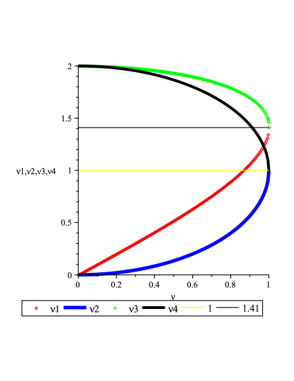
Figure 1: Parameters $\nu_{1}^{\mp},\nu_{2}^{\mp}$ as functions of $\nu$.

In order to understand the physical meaning of the double-valued dependence of $m_{1}$ and $m_{2}$ on $m$, $m_{max}$ we consider the geometric theory with a limited mass. Substituting into formula (66) defining the masses $m_{1},m_{2},m_{3},m_{4}$, the value $\cos\mu=\sqrt{1-\frac{m^{2}}{M^{2}}}$, we obtain

$$m_{1}=\sqrt{2}M\sqrt{1-\sqrt{1-m^{2}/M^{2}}};$$ (85)

$$m_{2}=M\left(1-\sqrt{1-m^{2}/M^{2}}\right);$$ (86)

$$m_{3}=\sqrt{2}M\sqrt{1+\sqrt{1-m^{2}/M^{2}}};$$ (87)

$$m_{4}=M\left(1+\sqrt{1-m^{2}/M^{2}}\right).$$ (88)

It is quite obvious that expressions (85)–(88) and (81), (82) coincide to the change of variable $M\leftrightarrow m_{max}$:

$$\frac{m_{1}^{2}}{2m_{2}}=\frac{m_{3}^{2}}{2m_{4}}=M\longleftrightarrow\frac{{m_{1}^{\mp}}^{2}}{2m_{2}^{\mp}}=m_{max}.$$

This means that if the parameter $m_{max}$ is introduced in the algebraic theory and identified with the maximal mass $M$ from Kadyshevsky’s geometric theory, it turns out that the algebraic model also contains the description of “exotic” particles, which was earlier considered to be the capability of the geometric approach. In other words, it can be established that, similar to the parameters $m_{1}$ and $m_{2}$ in the geometric theory which participate in description of ordinary particles, the parameters $m_{1}^{-}$, $m_{2}^{-}$ play the same role in the algebraic model (they correspond to the lower branches of the plots, in Fig. 1). Similarly, the parameters $m_{3}$, $m_{4}$, are used for description of exotic particles in the geometric model, and in the algebraic model the corresponding parameters are $m_{1}^{+}$, $m_{2}^{+}$ (upper branches of the plots, $\nu_{1}^{+}$, $\nu_{2}^{+}$). The regions of variation of the physical mass $m$ and the parameters $m_{1}$ and $m_{2}$ are

$$0\leq m\leq m_{max};\qquad m\leq m_{1}\leq 2m_{max};\qquad 0\leq m_{2}\leq 2m_{max}.$$ (89)

They correspond to the following regions on the plot, respectively:

$$0\leq\nu\leq 1;\qquad\nu\leq\nu_{1}\leq 2;\qquad 0\leq\nu_{2}\leq 2.$$

Apparently, in the algebraic interpretation these constraints define the region of unbroken $\cal PT$ -symmetry of the model corresponding to (76). The point $m=m_{max}$ ($\nu=1$ on the plot) is a special case: it corresponds to the maximon. At this point of the plot we have $\nu_{1}^{-}=\nu_{1}^{+}=\sqrt{2}$ and $\nu_{2}^{-}=\nu_{2}^{+}=1$. Note that with the appearance of exotic particles the theoretical essence of the maximon does not change either physically or mathematically. It still plays the role of the particle with the maximal mass. Note that in the geometric model the appearance of “exotic” particles was considered to be a consequence of the approach itself in which the new unusual particle properties were connected with the new degree of freedom in the theory, the sign of the momentum component $p_{5}$ ($\epsilon=p_{5}/|p_{5}|=\pm 1$ (see [2, 11]). It can be seen, however, that in the algebraic approach the introduction of the parameter $m_{max}$ also makes it possible to include the description of “exotic” particles in the theory. Thus, the appearance of “exotic” particles is directly connected with the non-Hermitian character of the considered Hamiltonian [69], [70].

This also makes it possible to specify the region of $\cal PT$-symmetry of the model. It can be seen from Fig. 2 that the region of $\cal PT$-symmetry of the Hamiltonian

$${\hat{H}}=\overrightarrow{\hat{\alpha}}\overrightarrow{p}+\hat{\beta}\left(m_{1}^{\mp}+m_{2}^{\mp}\gamma_{5}\right)$$ (90)

in the plane $m_{1},m_{2}$ is determined by three groups of inequalities (with account of the possible change of sign of the parameter $m_{2}$):

$$I.\,\,\,\,\,\,\,\,\,\,\,\,\,\,\,\,\,\,m_{1}/\sqrt{2}\leq m_{2}\leq m_{1},$$

$$II.-m_{1}/\sqrt{2}\leq m_{2}\leq m_{1}/\sqrt{2},$$

$$III.\,\,\,\,\,\,\,\,-m_{1}\leq m_{2}\leq-m_{1}/\sqrt{2}.$$

It should be underlined that, unlike [58], here the region of $\cal PT$-symmetry is defined in detail and it is demonstrated that while the central subregion $II$ corresponds to an ordinary particle, subregions $I$ and $III$ correspond to exotic particles. Thus, it is absolutely clear that expression (76) cannot be considered as the only constraint in the theory, and introducing the parameter $m_{max}$ and taking into account inequality (78) makes it possible to specify more precisely the region of $\cal PT$-symmetry of the model [70].

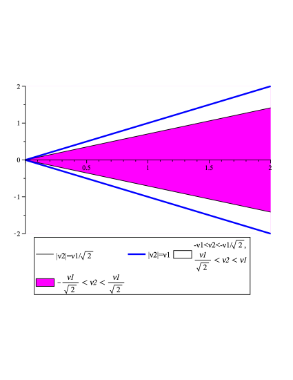
Figure 2: The parametric region of unbroken $\cal PT$-symmetry ${m_{1}}^{2}\geq{m_{2}}^{2}$ for Hamiltonian (90) consists of three subregions. Shaded subregion $II$ corresponds to ordinary particles, and two neighboring subregions $I$ and $III$ correspond to exotic fermions.

The following fact is surprising: in the algebraic model for any pre-set values of $m_{1}$ and $m_{2}$, with account of (80), constraint (78) appears automatically, similar to the geometric theory. Indeed, let us consider the parameter [72]

$$\xi=\frac{m_{1}}{M}=\frac{2m_{2}}{m_{1}}.$$ (91)

Taking into account (80), we have

$$\frac{m_{2}}{M}=\frac{\xi^{2}}{2}.$$ (92)

Figure 3 shows the dependence of the quantities $m/m_{1}$, $M/m_{1}$ and $m/M$ on the parameter $\xi=\frac{m_{1}}{M}=\frac{2m_{2}}{m_{1}}.$ In particular, it can be seen that the function $m/M$ has a maximum at the point $m=M$. The maximal particle mass $m=M$ is achieved when the auxiliary mass parameters satisfy the following relation: $m_{2}=m_{1}/\sqrt{2}.$ One can find the parameters $m_{1}$ and $m_{2}$ for which there exists the limiting transition to the standard Dirac equation up to this value of the parameter. Higher values of $m_{2}$ bring us to the decreasing branch of the curve $m/M$, and there is no Dirac limit in this region, while at the point $m_{1}=m_{2}=2m_{max}$ the value of $m$ is again equal to zero. Similar to Fig. 1, this means that now the case of massless particles, for example, corresponds to the two points: $m_{1}=m_{2}=0$ and $m_{1}=m_{2}=2M$. In the first case, we have the description of ordinary massless fermions, and the second case should be interpreted as the description of their exotic partners. This yields that the region $m_{1}<\sqrt{2}m_{2}$ corresponds to the description of “exotic” particles for which there is no transition to the Hermitian limit. In this case, the point $m_{2}=m_{1}=2M$ corresponds to massless exotic fermions.

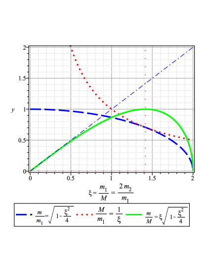
Figure 3: Ratios $m/M$, $M/m_{1}$ and $m/m_{1}$ as functions of $\xi=\frac{m_{1}}{M}=\frac{2m_{2}}{m_{1}}.$

Expressions (81), (82) make it possible to consider the “physical” approach in this algebraic model [75], [76], i.e., to answer the question posed earlier: how can a particular particle be described using Hamiltonian (69)? In other words, how can one find the parameters $m_{1}$, $m_{2}$ for the particle description in the framework of the algebraic model using the known physical mass $m$ of the particle? It was already noted that it is impossible to answer this question unambiguously using condition (75) alone. If the parameter $m_{max}$ is introduced, the answer follows from Eqs. (81), (82). Actually, by doing so, the transition is made from the two-parametric problem defined by Hamiltonian (69) with the parameters $m_{1}$, $m_{2}$, to the two-parametric problem with the parameters $m$, $m_{max}$. This proves once more the necessity of introducing the parameter $m_{max}$, and taking into account (78).

Let us consider the algebraic model describing the whole fermion spectrum [70–76] in this context. The question on the unique character of for all particles arises. It can be assumed from physical considerations that the model in which $m_{max}$ is unique for all particles is more preferable. Then it is logical to conclude that this unique $m_{max}$, is the maximon mass and should correspond to the limiting mass $M$ in the geometric approach. This turns out to be possible because, as it was already indicated above, the Hamiltonians and evolution equations in these two models coincide to notation. In other words, it is necessary to assume the equality of $m_{max}$ and $M$ in the theory describing the mass spectrum of elementary particles from physical considerations. Since the value of $M$ should follow from experiment, the postulate of the equality of $m_{max}$ and $M$ results in the physical constraint on the mass spectrum $m_{max}=M$, along with the condition $m_{max}=\frac{m_{1}^{2}}{2m_{2}}$ in the algebraic model.

Thus, the connection of this algebraic model and the geometric theory with a maximal mass is established once again [1, 2, 7–17].

4 Scalar product in pseudo-Hermitian model

Since the considered Hamiltonian is non-Hermitian (pseudo-Hermitian, see (71)), it is necessary to introduce a new scalar product defined by the operator $\cal C$. For this purpose we rewrite the mass term of the Hamiltonian in the form

$$\hat{\beta}(m_{1}+m_{2}\gamma_{5})=\hat{\beta}m(\mathrm{ch}\alpha+\gamma_{5}\mathrm{sh}\alpha)=\hat{\beta}m\exp{(\gamma_{5}\alpha)},$$ (93)

where $\mathrm{ch}\alpha=m_{1}/m.$ Now we can write the original Hamiltonian as follows:

$$\hat{H}=\hat{\overrightarrow{\alpha}}\overrightarrow{p}+\hat{\beta}m\exp({\gamma_{5}\alpha}),$$ (94)

and the Hermitian conjugate transpose Hamiltonian as

$$\hat{{H^{\dagger}}}=\hat{\overrightarrow{\alpha}}\overrightarrow{p}+\hat{\beta}m\exp({-\gamma_{5}\alpha}).$$ (95)

Using the commutation rules for the matrices ${\gamma}_{5}$, $\hat{\vec{\alpha}}$ and $\hat{\beta}$ it can be easily shown that

$$e^{\alpha\gamma_{5}/2}{\hat{H}}={\hat{H_{0}}}e^{\alpha\gamma_{5}/2}={\hat{H_{0}}}\eta$$ (96)

and

$$e^{-\alpha\gamma_{5}/2}\hat{H^{\dagger}}={\hat{H_{0}}}e^{-\alpha\gamma_{5}/2}={\hat{H_{0}}}{\eta}^{-1},$$ (97)

where the following notation:

$$\hat{H}_{0}=\overrightarrow{\hat{\alpha}}\overrightarrow{p}+\hat{\beta}m,$$

corresponding to the original free Dirac Hamiltonian is introduced, and

$$\eta=e^{\alpha\gamma_{5}/2}.$$ (98)

It can be easily seen from (94) and (97) that the Hermitian Hamiltonian $\hat{H}_{0}$ and the Hamiltonians $\hat{H}$, $\hat{H}^{\dagger}$ are connected by the non-unitary transformation $\eta$. (See the geometric theory in de Sitter space [77] where a similar transformation is unitary, for comparison).

It is also obvious that

$$\eta_{0}{\hat{H}}{\eta_{0}}^{-1}={\hat{H}^{\dagger}},$$ (99)

where the operator $\eta_{0}=e^{\alpha\gamma_{5}}={\eta}^{2}$ defines the pseudo-Hermitian properties of the Hamiltonian. Following [32], we can define the following operator:

$${\cal C}={\eta_{0}}^{-1}{\cal P}=e^{-\alpha\gamma_{5}}\gamma_{0}.$$ (100)

Using the standard representation of $\gamma$-matrices, the operator ${\cal C}$ can be written in the matrix form,

$${\cal C}=\left(\begin{array}[]{cc}0&I\frac{m_{1}^{\mp}-m_{2}^{\mp}}{m}\\ I\frac{m_{1}^{\mp}+m_{2}^{\mp}}{m}&0\end{array}\right),$$ (101)

where $I=\left(\begin{array}[]{cc}1&0\\ 0&1\end{array}\right)$. Note that the operator ${\cal C}$ ${\cal C}$ in notation (71) or (101) has a simpler form and is more convenient than the corresponding expression in [58], since here (see [71, 76]) it is obtained explicitly, while in [58] this operator was constructed via the iteration method and written in the integral form.

It can be easily proved that the scalar product constructed using ${\cal C}$-operator (101) in a standard way [32] is positive definite. Indeed (see [71, 76]), let us write an arbitrary vector in the modified theory,

$$\widetilde{\psi}=\left(\begin{array}[]{cc}x+iy&{}\hfil\\ u+iv&{}\hfil\\ z+iw&{}\hfil\\ t+ip&{}\hfil\end{array}\right).$$

It can further be proved by direct calculations using representation (101) for the operator ${\cal C}$, that the norm of the vector $\widetilde{\psi}$ in the considered theory with the modified scalar product is given by the expression

$$\langle{}\overline{\widetilde{\psi}}{\cal C}|\widetilde{\psi}\rangle=\frac{m_{1}+m_{2}}{m}(x^{2}+y^{2})+\frac{m_{1}+m_{2}}{m}(u^{2}+v^{2})+\frac{m_{1}-m_{2}}{m}(z^{2}+w^{2})+\frac{m_{1}-m_{2}}{m}(t^{2}+p^{2}).$$ (102)

This expression is positive definite in region (76) of ${\cal PT}$-symmetry of the considered theory, i.e., for $m_{1}\geq m_{2}$.

It can also be easily seen that the average values of Hamiltonian (90) in the modified scalar product are real. Let us write

$$\langle{}\overline{\widetilde{\psi}}{\cal C}\hat{H}|\widetilde{\psi}\rangle=\langle{}\overline{\widetilde{\psi}}e^{-\alpha\gamma_{5}}\gamma_{0}\bigl{(}\overrightarrow{\hat{\alpha}}\overrightarrow{p}+\hat{\beta}me^{\alpha\gamma_{5}}\bigr{)}\widetilde{\psi}\rangle.$$ (103)

Taking the Hermitian conjugate transpose and performing elementary commutations similar to (94), (97), we prove that this expression is real.

Let us consider the problem of finding eigenvalues and eigenvectors of Hamiltonian (69) [71],

$$\hat{H}\widetilde{\psi}=E\widetilde{\psi}.$$

Using the standard representation of $\gamma$-matrices, we write $\hat{H}$ in the matrix representation,

$$\hat{H}=\left(\begin{array}[]{cccc}m_{1}&0&p_{3}-m_{2}&p_{1}-ip_{2}\\ 0&m_{1}&p_{1}+ip_{2}&-m_{2}-p_{3}\\ m_{2}+p_{3}&p_{1}-ip_{2}&-m_{1}&0\\ p_{1}+ip_{2}&m_{2}-p_{3}&0&-m_{1}\\ \end{array}\right),$$

where $p_{i}$ are the momentum components. The condition

$$\det{(\hat{H}-E)}=(-E^{2}+{m_{1}}^{2}-{m_{2}}^{2}+{p_{\bot}}^{2}+{p_{3}}^{2})^{2}=0$$

makes it possible to determine the eigenvalues of the energy $E$,

$$\emph{E}=\pm\sqrt{{m_{1}}^{2}-{m_{2}}^{2}+{p_{\bot}}^{2}+{p_{3}}^{2}},$$ (104)

where $p_{\bot}=\sqrt{{p_{1}}^{2}+{p_{2}}^{2}}$ and ${m_{1}}^{2}-{m_{2}}^{2}=m^{2}$. It can be seen that the values of $E$ coincide with the eigenvalues of the Hermitian operator $\hat{H_{0}}$.

Let us consider the wave function describing a free particle with a certain energy and momentum. It can be represented as a plane wave,

$$\widetilde{\psi}=\frac{1}{\sqrt{2E}}\widetilde{u}e^{-ipx}.$$ (105)

Here, the amplitude $\widetilde{u}$ is a bispinor and satisfies the algebraic equations

$$\left(\gamma{p}-me^{\gamma_{5}\vartheta}\right)\widetilde{u}=0;$$ (106)

$$\overline{\widetilde{u}}\left(\gamma{p}-me^{-\vartheta\gamma_{5}}\right)=0,$$ (107)

where $\overline{\widetilde{u}}={\widetilde{u}}^{*}\gamma_{0}$. The solutions to Eqs. (106), (107) can be represented in the form (see [71, 76])

$$\widetilde{u}=\sqrt{2m}\left(\begin{array}[]{c}A_{1}w\\ A_{2}w\\ \end{array}\right);$$ (108)

$$\overline{\widetilde{u}}=\sqrt{2m}\left(\begin{array}[]{cc}A_{1}^{*}w^{*},&-A_{2}^{*}w^{*}\\ \end{array}\right),$$ (109)

where $A_{1}$, $A_{2}$ are defined by the expressions

$$A_{1}=\mathrm{ch}\frac{\alpha}{2}\mathrm{ch}\frac{\beta}{2}+\mathrm{sh}\frac{\alpha}{2}\mathrm{sh}\frac{\beta}{2}(\textbf{n}\overrightarrow{{\sigma}});$$

$$A_{2}=\mathrm{sh}\frac{\alpha}{2}\mathrm{ch}\frac{\beta}{2}+\mathrm{ch}\frac{\alpha}{2}\mathrm{sh}\frac{\beta}{2}(\textbf{n}\overrightarrow{{\sigma}}).$$

Here, $\mathrm{ch}\,\alpha=m_{1}/m$,   $\mathrm{sh}\,\alpha=m_{2}/m$ and $\mathrm{ch}\,\beta=\emph{\emph{\emph{E}}}/m$,   $\mathrm{sh}\,\beta=p/m$, and $w$ is the two-component spinor satisfying the condition

$$\overrightarrow{\sigma}{\textbf{n}}w_{\zeta}=\zeta w_{\zeta}$$ (110)

and the normalization relations

$$w^{*}w=1.$$

We recall here the standard notation: $\overrightarrow{\sigma}$ are the Pauli matrices with the dimension $2\times 2$, and $\textbf{n}=\textbf{p}/p$ is the unit vector along the momentum.

Solving Eq. (110), we have

$$w_{1}=\left(\begin{array}[]{c}e^{-i\varphi/2}\cos\theta/2\\ e^{i\varphi/2}\sin\theta/2\\ \end{array}\right),\,\,\,\,\,w_{-1}=\left(\begin{array}[]{c}-e^{-i\varphi/2}\sin\theta/2\\ e^{i\varphi/2}\cos\theta/2\\ \end{array}\right),$$

where $\theta$ and $\varphi$ are the polar and azimuthal angles defining the direction of n relative to the axes $x_{1},x_{2},x_{3}$.

Satisfaction of the following condition can be easily verified by direct calculation:

$$\overline{\widetilde{u}}\widetilde{u}=2m.$$

This result is quite expected, since there exists the transformation connecting the bispinor amplitudes of the modified equations $\overline{\widetilde{u}},\widetilde{u}$ and the corresponding solutions to the original Dirac equations,

$$\widetilde{u}=e^{-\gamma_{5}\alpha/2}u$$

$$\overline{\widetilde{u}}=\overline{u}e^{\gamma_{5}\alpha/2}.$$

Taking into account that the Dirac bispinors are normalized using the relation $\overline{u}u=2m$ (see [78]), we have

$$\overline{\widetilde{u}}\widetilde{u}=\overline{u}u=2m.$$ (111)

In conclusion, we note that it is interesting to observe a natural appearance of the operator ${\cal C}$ in form (100) in the considered algebraic theory with $\gamma_{5}$-mass extension (see [73]). For this purpose we write the modified Dirac equation and the conjugate equation in $x$ representation,

$$\left(i\gamma^{\mu}\partial_{\mu}-(m_{1}+m_{2}\gamma_{5})\right)\widetilde{\psi}=0$$ (112)

$$\overline{\widetilde{\psi}}\left(i\gamma^{\mu}\partial_{\mu}+(m_{1}-m_{2}\gamma_{5})\right)=0.$$ (113)

Let us rewrite them as

$$\left(i\gamma^{\mu}\partial_{\mu}-m\exp{(\alpha\gamma_{5}))}\right)\widetilde{\psi}=0$$ (114)

$$\overline{\widetilde{\psi}}\left(i\gamma^{\mu}\overleftarrow{\partial_{\mu}}+m\exp{(-\alpha\gamma_{5})}\right)=0.$$ (115)

Now let us multiply the first equation by from $\overline{\widetilde{\psi}}e^{-\alpha\gamma_{5}}$ the left, and the second equation by from $e^{\alpha\gamma_{5}}\widetilde{\psi}$ the right. Summing the first and the second equations and performing simple commutations, we obtain the continuity law for the current density,

$$\partial_{\mu}\left(\overline{\widetilde{\psi}}e^{-\alpha\gamma_{5}}\gamma_{\mu}\widetilde{\psi}\right)=0.$$ (116)

In this case, the current $j_{\mu}$ is defined by the following formula:

$$j_{\mu}=\overline{\widetilde{\psi}}e^{-\alpha\gamma_{5}}\gamma_{\mu}\widetilde{\psi}.$$ (117)

Taking into account that $\int_{V_{\infty}}\textrm{div}\overrightarrow{j}dV=0,$ we obtain the time conservation of the quantity $\int_{V_{\infty}}j_{0}dV\equiv\int_{V_{\infty}}\rho dV.$ Then, using the transformations from [73], we have

$$\int_{V_{\infty}}\rho dV=\int\overline{\widetilde{\psi}}e^{-\alpha\gamma_{5}}\gamma_{0}\widetilde{\psi}\ dV=\int\overline{\widetilde{\psi}}\eta_{0}^{-1}{\cal P}\widetilde{\psi}dV=\int\overline{\widetilde{\psi}}{\cal C}\widetilde{\psi}dV=1.$$

Thus, the quantity $\overline{\widetilde{\psi}}{\cal C}\widetilde{\psi}$ has the meaning of the probability amplitude and it can be seen that the scalar product contains the operator ${\cal C}=\eta_{0}^{-1}{\cal P}$. Hence, in this case the operator ${\cal C}$, coinciding with operator (71) constructed in strict agreement with the theories [32, 57] appears in a natural way.

5 $\gamma_{5}$-modified Dirac model in a homogeneous magnetic field

It is known that exact solutions to Dirac wave equation are the basis of relativistic quantum mechanics and quantum electrodynamics of spinor particles in external magnetic fields. The obtaining, analyzing, and using its exact solutions is an important aspect of development of this field of science. Just a few physically important exact solutions to the original Dirac equations are known. They include, in particular, an electron in a Coulomb field, a homogeneous magnetic field, and a plane wave field. Exact solutions to the relativistic wave equation, i.e., single-particle wave functions, make it possible to apply the approach known as the Furry picture which is based on their use. This very fruitful method of investigation includes the study of particle interaction with an external field independently of the field strength value (see [78]). It is interesting to study non-Hermitian extensions of the Dirac model which represent alternative formulations of relativistic quantum mechanics and try to implement the Furry picture method in them [72–74].

Let us consider the homogeneous magnetic field $\textbf{H}=(0,0,H)$ directed along the axis $x_{3}$ ($H>0$). The electromagnetic field potentials in gauge [78] can be chosen in the following form: $A_{0}=0,\,\,A_{1}=0,\,\,A_{2}=Hx_{1},\,\,A_{3}=0.$ Let us write the modified Dirac equation in the form

$$\left(\gamma_{\mu}{\cal P^{\mu}}-me^{\vartheta\gamma_{5}}\right)\widetilde{\Psi}=0,$$ (118)

where ${\cal P^{\mu}}=i\partial_{\mu}-eA_{\mu}$ ; $e=-|e|,$ and we use $\gamma$-$\gamma$-matrices in the standard representation. In the considered region the integrals of motion ${\cal P}_{0},\,{\cal P}_{2}$ and ${\cal P}_{3}$ mutually commute, $[{\cal D},{\cal P}_{0}]=0$, $[{\cal D},{\cal P}_{2}]=0$, $[{\cal D},{\cal P}_{3}]=0$ where ${\cal D}=(\gamma_{\mu}{\cal P}^{\mu}-me^{\vartheta\gamma_{5}})$.

Let us represent the function $\widetilde{\Psi}$ in the form

$$\widetilde{\Psi}=\left(\begin{array}[]{c}\psi_{1}\\ \psi_{2}\\ \psi_{3}\\ \psi_{4}\\ \end{array}\right)e^{-iEt}$$

and use the Hamiltonian form of the Dirac equations,

$$H\widetilde{\psi}=E\widetilde{\psi},$$ (119)

where

$$H=(\overrightarrow{\alpha}\textbf{{\cal P}})+\beta m_{1}+\beta\gamma_{5}m_{2}.$$

Changing the variables [78]

$$\psi_{i}(x_{1},x_{2},x_{3})=e^{ip_{2}x_{2}+ip_{3}x_{3}}\Phi_{i}(x_{1}),$$

where $i=1,2,3,4,$$i=1,2,3,4,$ we obtain the following system of equations [73]:

$$(E\mp m_{1})\Phi_{1,3}+iR_{2}\Phi_{4,2}-(p_{3}\mp m_{2})\Phi_{3,1}=0;$$ (120)

$$(E\mp m_{1})\Phi_{2,4}+iR_{1}\Phi_{3,1}+(p_{3}\pm m_{2})\Phi_{4,2}=0.$$ (121)

Here, $R_{1}=\left[\frac{\partial}{\partial x_{1}}-(p_{2}+{eH})\right],$ $R_{2}=\left[\frac{\partial}{\partial x_{1}}+(p_{2}+{eH})\right],$ the upper sign is related to the components of the wave function with the first index, and the lower sign, to the components of the wave function with the second index.

It is convenient to use the following dimensionless variable:

$$\rho=\sqrt{\gamma}x_{1}+p_{2}/\sqrt{\gamma},$$ (122)

where $\gamma=|e|H$, then Eqs. (120), (121) take the form

$$(E\mp m_{1})\Phi_{1,3}+i\sqrt{\gamma}\left(\frac{d}{d\rho}+\rho\right)\Phi_{4,2}-(p_{3}\mp m_{2})\Phi_{3,1}=0;$$ (123)

$$(E\mp m_{1})\Phi_{2,4}+i\sqrt{\gamma}\left(\frac{d}{d\rho}-\rho\right)\Phi_{3,1}+(p_{3}\pm m_{2})\Phi_{4,2}=0.$$ (124)

The general solution to this system can be represented in the following form:

$$u_{n}(\rho)=\left(\frac{\gamma^{1/2}}{2^{n}n!\pi^{1/2}}\right)e^{-\rho^{2}/2}H_{n}(\rho),$$

where $H_{n}(x)$ are the standard Hermite polynomials,

$${\mathit{H}}_{n}(x)=(-1)^{n}e^{x^{2}/2}\frac{d^{n}}{dx^{n}}e^{-x^{2}/2},$$

and $n=0,1,2..$.

Note that this Hermite functions satisfy the following recurrence relations:

$$\left(\frac{d}{d\rho}+\rho\right)u_{n}=(2n)^{1/2}u_{n-1};$$ (125)

$$\left(\frac{d}{d\rho}-\rho\right)u_{n-1}=-(2n)^{1/2}u_{n}.$$ (126)

It can be easily seen from (125), (126) that

$$\left(\frac{d}{d\rho}-\rho\right)\left(\frac{d}{d\rho}+\rho\right)u_{n}=-2nu_{n}$$

and, therefore (see, e.g., [78]),

$$R_{1}R_{2}=-2\gamma n.$$ (127)

Substituting into (123), (124) the expression

$$\Phi=\left(\begin{array}[]{c}C_{1}u_{n-1}(\rho)\\ iC_{2}u_{n}(\rho)\\ C_{3}u_{n-1}(\rho)\\ iC_{4}u_{n}(\rho)\\ \end{array}\right),$$

it can be obtained that the coefficients $C_{i}\,(i=1,2,3,4)$ are determined by the algebraic equations

$$(E\mp m_{1})C_{1,3}-(2\gamma n)^{1/2}C_{4,2}-(p_{3}\mp m_{2})C_{3,1}=0;$$

$$(E\mp m_{1})C_{2,4}-(2\gamma n)^{1/2}C_{3,1}+(p_{3}\pm m_{2})C_{4,2}=0.$$

Let us find the energy spectrum of this non-Hermitian Hamiltonian by equating to zero the determinant of this system,

$$E=\pm\sqrt{{m_{1}}^{2}-{m_{2}}^{2}+2\gamma n+{p_{3}}^{2}},$$ (128)

where $n=0,1,2..$, taking into account that $m^{2}={m_{1}}^{2}-{m_{2}}^{2}$, we can see that this result (see also (104)) coincides with the eigenvalues of the Hermitian Hamiltonian describing Landau relativistic levels (see, e.g., [78]).

The coefficients $C_{i}$ can be determined if we use the third component of the polarization tensor in the direction of the magnetic field as the polarization operator [78],

$$\mu_{3}=m_{1}\sigma_{3}+\rho_{2}[\vec{\sigma}\vec{{\cal P}}]_{3},$$ (129)

where the matrices

$$\sigma_{3}=\left(\begin{array}[]{cc}I&0\\ 0&-I\\ \end{array}\right);\,\,\,\,\,\rho_{2}=\left(\begin{array}[]{cc}0&-iI\\ iI&0\\ \end{array}\right).$$

It can be easily seen that the bispinor $C$ can be written in the form

$$\left(\begin{array}[]{c}C_{1}\\ C_{2}\\ C_{3}\\ C_{4}\\ \end{array}\right)=\frac{1}{2\sqrt{2}}\left(\begin{array}[]{c}\mathrm{ch}(\vartheta/2)\Phi_{1}+\mathrm{sh}(\vartheta/2)\Phi_{3}\\ \mathrm{ch}(\vartheta/2)\Phi_{2}+\mathrm{sh}(\vartheta/2)\Phi_{4}\\ \mathrm{sh}(\vartheta/2)\Phi_{1}+\mathrm{ch}(\vartheta/2)\Phi_{3}\\ \mathrm{sh}(\vartheta/2)\Phi_{2}+\mathrm{ch}(\vartheta/2)\Phi_{4},\\ \end{array}\right),$$ (130)

where

$$\Phi_{1}=\sqrt{1+\zeta m/p_{\bot}}\sin(\pi/4+\lambda/2)$$

$$\Phi_{2}=\zeta\sqrt{1-\zeta m/p_{\bot}}\sin(\pi/4-\lambda/2)$$

$$\Phi_{3}=\zeta\sqrt{1+\zeta m/p_{\bot}}\sin(\pi/4-\lambda/2)$$

$$\Phi_{4}=\sqrt{1-\zeta m/p_{\bot}}\sin(\pi/4+\lambda/2).$$

Here, $\mu_{3}\psi=\zeta k\psi$, $k=\sqrt{{p_{\bot}}^{2}+m^{2}}$ and $\zeta=\pm 1$, which corresponds to the following fermion spin orientation: along $(+1)$ and opposite $(-1)$ to the magnetic field, and the parameter $\lambda$ satisfies the relation $\cos{\lambda}=p_{3}/E.$ The functions $\mathrm{sh}(\vartheta/2)$ and $\mathrm{ch}(\vartheta/2)$ are defined by the relations

$$\mathrm{ch}\vartheta=m_{1}/m;\,\,\,\,\mathrm{sh}\vartheta=m_{2}/m.$$ (131)

It should be pointed out that the use of the exact solution to the Dirac equation in a magnetic field has recently yielded a number of interesting experimental results. In particular, in [79, 80] exact agreement between this relativistic model and different combinations of Jaynes–Cummings (JC) [79] and anti-Jaynes–Cummings (AJC) [80] interactions was found. These nontrivial facts imply important results which are widely used in quantum optics.

6 Modified non-Hermitian Dirac-Pauli model in a magnetic field

In this section, we consider the description of motion of Dirac particles with magnetic momentum other than the Bohr magneton [3, 4]. It was shown by Schwinger [81] that the Dirac equation for particles in an external electromagnetic field $A^{ext}$ with account of radiative corrections can be represented as

$$\left(\hat{{\cal P}}\gamma-m\right)\Psi(x)-\int{\cal M}(x,y|A^{ext})\Psi(y)dy=0,$$ (132)

where ${\cal M}(x,y|A^{ext})$ is the mass operator of fermions in an external field. The modified equation (see, e.g. [78]) can be obtained from Eq. (132) by expanding the mass operator in $eA^{ext}$ series to the first order with respect to the field. This equation possesses relativistic covariance and agrees with the phenomenological Pauli equation obtained in his early papers.

Let us consider the model of massive fermions with $\gamma_{5}$-mass extension $m\rightarrow m_{1}+\gamma_{5}m_{2}$ , taking into account the interaction of their charges and anomalous magnetic moments with the electromagnetic field $F_{\mu\nu}$:

$$\left(\gamma^{\mu}{\cal P}_{\mu}-m_{1}-\gamma_{5}m_{2}-\frac{\Delta\mu}{2}\sigma^{\mu\nu}F_{\mu\nu}\right)\widetilde{\Psi}(x)=0,$$ (133)

where $\Delta\mu=(\mu-\mu_{0})=\mu_{0}(g-2)/2$. Here, $\mu$ is the magnetic moment of the fermion, $g$ is the gyromagnetic factor of the fermion, $\mu_{0}=|e|/2m$ is the Bohr magneton, and and $\sigma^{\mu\nu}=i/2(\gamma^{\mu}\gamma^{\nu}-\gamma^{\nu}\gamma^{\mu})$. Thus, the phenomenological constant $\Delta\mu$ introduced by Pauli is a part of the equation and can be interpreted from the point of view of the quantum field theory.

The Hamiltonian form of Eq. (133) for fermions in a homogeneous magnetic field is [3, 4]:

$$i\frac{\partial}{\partial t}\widetilde{\Psi}(r,t)=H_{\Delta\mu}\widetilde{\Psi}(r,t),$$ (134)

where

$$H_{\Delta\mu}=\vec{\alpha}\vec{{\cal P}}+\beta(m_{1}+\gamma_{5}m_{2})+\Delta\mu\beta(\vec{\sigma}\textbf{H}).$$ (135)

In particular, taking into account the quantum electrodynamic contribution into the anomalous magnetic moment of the electron to $e^{2}$, we have $\Delta\mu=\frac{\alpha}{2\pi}\mu_{0}$, where $\alpha=e^{2}=1/137$ is the fine structure constant, and it is still assumed that the external field potential satisfies the free Maxwell equation.

It should be noted that here the operator of fermion spin projection onto the direction of its motion $\overrightarrow{\sigma}\overrightarrow{{\cal P}}$ does not commute with Hamiltonian (135) and therefore, is not an integral of motion. The operator commuting with the Hamiltonian is $\mu_{3}$ (see (129)). Thus, the wave function $\widetilde{\psi}$ is the eigenfunction of polarization operator (129) and Hamiltonian (135). Therefore, we have

$$\mu_{3}\psi=\zeta k\psi,\,\,\,\mu_{3}=\left(\begin{array}[]{cccc}m_{1}&0&0&{\cal P}_{1}-i{\cal P}_{2}\\ 0&-m_{1}&-{\cal P}_{1}-i{\cal P}_{2}&0\\ 0&-{\cal P}_{1}+i{\cal P}_{2}&m_{1}&0\\ {\cal P}_{1}+i{\cal P}_{2}&0&0&-m_{1}\\ \end{array}\right),$$ (136)

where $\zeta=\pm 1$ characterizes the fermion spin projection onto the magnetic field direction, and

$$H_{\Delta\mu}\widetilde{\psi}=E\widetilde{\psi},$$

$$H_{\Delta\mu}=\left(\begin{array}[]{cccc}m_{1}+H\Delta\mu&0&{\cal P}_{3}-m_{2}&{\cal P}_{1}-i{\cal P}_{2}\\ 0&m_{1}-H\Delta\mu&{\cal P}_{1}+i{\cal P}_{2}&-m_{2}-{\cal P}_{3}\\ m_{2}+{\cal P}_{3}&{\cal P}_{1}-i{\cal P}_{2}&-m_{1}-H\Delta\mu&0\\ {\cal P}_{1}+i{\cal P}_{2}&m_{2}-{\cal P}_{3}&0&H\Delta\mu-m_{1}\\ \end{array}\right).$$ (137)

These calculations are similar to the calculations given in detail in the previous section. As a result, with the help of the modified Dirac–Pauli equation we can also find the exact values of the energy spectrum in the case of non-Hermitian Hamiltonian (135), (137) (see [3, 74]),

$$E(\zeta,p_{3},2\gamma n,H)=\pm\sqrt{{p_{3}}^{2}-{m_{2}}^{2}+\left[\sqrt{{m_{1}}^{2}+2\gamma n}+\zeta\Delta\mu H\right]^{2}},$$ (138)

and the eigenvalues of the polarization operator $\mu_{3}$

$$k=\sqrt{{m_{1}}^{2}+2\gamma n}.$$ (139)

It should be noted that formula (138) is satisfied not only for charged fermions but also for neutral particles with anomalous magnetic moment. In this case it is necessary to replace the value of the quantized transverse momentum of a charged particle in a magnetic field by the regular value, $2\gamma n\rightarrow{p_{1}}^{2}+{p_{2}}^{2}={p_{\bot}}^{2}$. As a result, we obtain [4, 73]:

$$E(\zeta,p_{3},p_{\bot},H)=\pm\sqrt{{p_{3}}^{2}-{m_{2}}^{2}+\left[\sqrt{{m_{1}}^{2}+{p_{\bot}}^{2}}+\zeta\Delta\mu H\right]^{2}}.$$ (140)

It can be seen from (140) that in the region of unbroken ${\cal PT}$-symmetry the energy spectrum is real if the particle spin is directed along the magnetic field, $\xi=+1$. It can be easily noted, however, that in the case $\zeta=-1$ (the fermion spin is directed opposite to the magnetic field) in the linear approximation with respect to the magnetic field strength, real values of the energy spectrum can be obtained only if the magnetic field strength is bounded by the following value:

$$H\leq\frac{{p_{0}}^{2}}{2\Delta\mu\,k},$$ (141)

where $p_{0}=\sqrt{m^{2}+{p_{\bot}}^{2}+{p_{3}}^{2}}$ is the regular Hermitian particle energy.

Therefore, expression (140) yields for $\zeta=-1$ and $p_{\bot}=p_{3}=0$, which corresponds to a fermion at rest, that $H\leq H_{max}$. In the linear approximation with respect to the magnetic field strength we can also find [3, 74]

$$H_{max}=\frac{m^{2}}{2m_{1}\Delta\mu}.$$ (142)

It can be easily obtained from (142) that the direct consequence of Eq. (138) is that the energy eigenvalues for $H\leq H_{max}$ are real. We can formulate a new condition of unbroken ${\cal PT}$-symmetry for the model of fermions with the non-Hermitian $\gamma_{5}$-mass extension and nonzero anomalous magnetic moment in a high-intensity external magnetic field using (142). This condition replaces condition (76) and can be written as

$${m_{1}}^{2}-{m_{2}}^{2}\geq 2m_{1}\Delta\mu H.$$ (143)

Thus, it can be seen that there exists the maximum magnetic field value $H_{max}$ such that if this value is exceeded for fermions at rest with $\zeta=-1$ it results in the loss of the real character of the energy spectrum.

It can be seen from (140) [4] that in the region of unbroken ${\cal PT}$-symmetry all energy levels are real if the particle spin is directed along the magnetic field, $\xi=+1$. If the spin is directed opposite to the magnetic field, $\xi=-1$, the energy of the fermion ground state $n=0$ has an imaginary part, as well as other lower energy levels. Figures 4 and 5 (see also [74]) show the energy values as functions of the parameter $x=m/M$ (see Fig. 4 for $\xi=+1$ and Fig. 5 for $\xi=-1$).

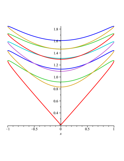
Figure 4: Dependence of $E(+1,0,0.4n,0.2)$ on parameter $x=m/M$ for the case $n=0,1,2,3,4$ and $\Delta\mu H=0.2.$

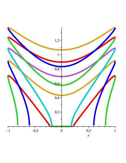
Figure 5: Dependence of $E(-1,0,0.4n,0.2)$ on parameter $x=m/M$ for the case $n=0,1,2,3,4$ and $\Delta\mu H=0.2.$

It can be easily seen that in the case $\Delta\mu=0$ regular expression for energy levels of a charged particle in an external field (128) (Landau levels) can be obtained from (138). It should be underlined that the expression similar to (138) can be obtained in the framework of the standard Dirac-Pauli approach, assuming $m_{2}=0$ and $m_{1}=m$ (Hermitian limit),

$$E(\zeta,p_{3},2\gamma n,H)=\pm\sqrt{{p_{3}}^{2}+\left[\sqrt{{m}^{2}+2\gamma n}+\zeta\Delta\mu H\right]^{2}}.$$ (144)

Note that the result similar to (144) was obtained earlier in [82] using the regular Hermitian approach to solution of the Dirac-Pauli equation. Direct comparison of modified formula (144) in the Hermitian limit (see [3, 4]) with the result obtained in [82] demonstrates their agreement. It can be easily seen that Eq. (138) contains the separate dependence on the parameters $m_{1}$ and $m_{2}$, rather than one parameter united in the physical mass (of the particle) $m=\sqrt{{m_{1}}^{2}-{m_{2}}^{2}}$, which differs essentially from the examples considered in the previous sections.

Thus, unlike (104) and (128), in this case the calculation of interaction of the fermion anomalous magnetic moment with the magnetic field makes it possible to put forward the question of the possibility of experimental observation of effects of $\gamma_{5}$-extension of the fermion mass.

Note that if it is assumed that $m_{2}=0$ and therefore $m_{1}=m$, we obtain, as it was already indicated earlier, the Hermitian limit. Taking into account expressions (81) and (82), however, it can be obtained that energy spectrum (138) is expressed in terms of the fermion mass $m$ and the maximal mass $M$. Thus, taking into account that the interaction of anomalous magnetic moment with the magnetic field eliminates degeneration with respect to the spin variable, we can obtain the energy of the ground state ($\zeta=-1$) in the form (see [3, 4])

$$E(-1,0,0,H,x)=m\sqrt{-\left({\frac{1\mp\sqrt{1-x^{2}}}{x}}\right)^{2}+\left(\frac{\sqrt{2}\sqrt{1\mp\sqrt{1-x^{2}}}}{x}-\frac{\Delta\mu H}{m}\right)^{2}},$$ (145)

where $x=m/M$, the upper sign corresponds to ordinary particles, and the lower sign corresponds to their “exotic” partners.

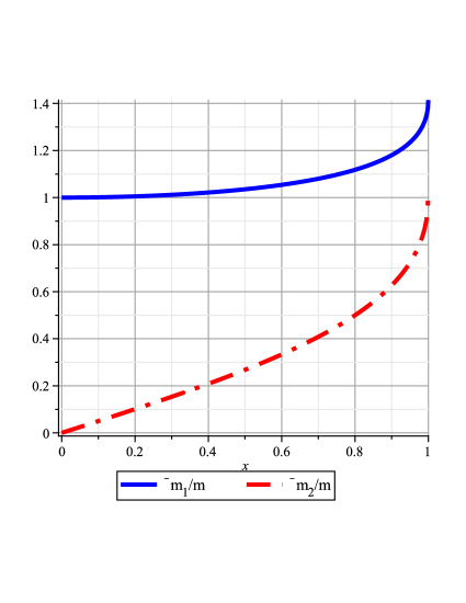
Figure 6: Dependence of $m^{-}_{1}/m,\,m^{-}_{2}/m$ on parameter $x=m/M.$

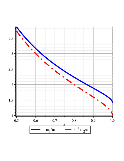
Figure 7: Dependence of parameters $m^{+}_{1}/m,\,m^{+}_{2}/m$ on value $x=m/M.$

Let us now pass over to more detailed examination of the ground state energy of fermions in an external field. Using the calculations given above (see (138)), the dependence of the energy of an ordinary fermion with the small mass $x=m/M\ll 1$ on the magnetic field strength $H$ can be obtained,

$$E(-1,0,0,H,x)=m\sqrt{1-\frac{\Delta\mu}{\mu_{0}}\frac{H}{H_{c}}(1+x^{2}/8+7x^{4}/128)+\left(\frac{\Delta\mu H}{m}\right)^{2}},$$ (146)

where $H_{c}=m^{2}/e=4.41\cdot 10^{13}$ G is the quantizing magnetic field for an electron [78].

At the same time, for the case of ”exotic” particles in the same limit $x\ll 1$ we have the result quite different from (146) (see [3, 4]),

$$E(-1,0,0,H,x)=m\sqrt{1-\frac{\Delta\mu}{\mu_{0}}\frac{2H}{xH_{c}}+\left(\frac{\Delta\mu H}{m}\right)^{2}}.$$ (147)

It can be seen from (147) that in this case the field corrections increase considerably, as $1/x=M/m\gg 1$. In the limit $m\rightarrow M$ the results for ordinary and exotic particles agree. Thus, combining these results we can write the following:

$$E(-1,0,0,H,x)=m\sqrt{1-\frac{\Delta\mu}{\mu_{0}}\frac{\sqrt{2}H}{xH_{c}}+\left(\frac{\Delta\mu H}{m}\right)^{2}}.$$ (148)

It can also be seen [73], that the change of parameters $m^{\mp}_{1}$ and $m^{\mp}_{2}$ takes place in such a way that at the point $x=1$ ($m=M$) the branches of the plots for the mass parameters of ordinary and exotic particles inter sect. It can be easily seen in Figs. 6 and 7 showing ${m}^{-}_{1,2}/m$ and $m^{+}_{1,2}/m$ as functions of $x=m/M$.

Since Eqs. (133) and formulas (138), (145), and (147) following from these equations are valid for practically any magnetic field intensities, it can be easily seen that for

$$H\sim\frac{\mu_{0}}{\Delta\mu}\frac{m}{m_{1}}H_{c}$$ (149)

we obtain $E_{0}\sim 0$. Thus, in a high-intensity magnetic field, consideration of the vacuum magnetic moment may result in an essential change of boundary of the energy spectrum between fermion and anti-fermion states. It should be pointed out that a considerable growth of this correction is connected with the possible contribution of the so-called exotic particles [3].

Let us consider the neutrino as an important example of applying the obtained expressions for the energy. Namely, in the case of ultracold polarized regular electron neutrinos, we obtain in the linear approximation with respect to the field (see (140))

$$E(-1,0,0,H,m_{\nu_{e}}/M\ll 1)=m_{\nu_{e}}\sqrt{1-\frac{\mu_{\nu_{e}}}{\mu_{0}}\frac{H}{H_{c}}}.$$ (150)

In the case of exotic electron neutrinos, however, the situation may change essentially,

$$E(-1,0,0,H,m_{\nu_{e}}/M\ll 1)=m_{\nu_{e}}\sqrt{1-\frac{\mu_{\nu_{e}}}{\mu_{0}}\frac{2MH}{m_{\nu_{e}}H_{c}}}.$$ (151)

It is well known [83, 84] that in the minimally extended SM one-loop radiative corrections contributing to the neutrino magnetic moment are proportional to the neutrino mass,

$$\mu_{\nu_{e}}=\frac{3}{8\sqrt{2}\pi^{2}}|e|G_{F}m_{\nu_{e}}=\left(3\cdot 10^{-19}\right)\mu_{0}\left(\frac{m_{\nu_{e}}}{1eV}\right),$$ (152)

where $G_{F}$ is the Fermi interaction constant, and $\mu_{0}$ is the Bohr magneton. The discussion of the problem of measurement of the neutrino mass (active or sterile components) yields that for the active neutrino of the model we have $\sum m_{\nu}=0.320eV$, while for the sterile neutrino, $\sum m_{\nu}=0.06eV$ [85].

Thus, the change of boundary of the region of unbroken ${\cal P}{\cal T}$ - symmetry due to the shift of the state with the lowest energy in the magnetic field can be estimated. Indeed, Eqs. (150) and (151) can be used to define the regions of ${\cal P}{\cal T}$ - symmetry preservation.

Let us consider the following neutrino parameters: the mass of the electron neutrino $m_{\nu_{e}}=1eV$ and magnetic moment (152). If it is assumed that the mass and magnetic moment of exotic neutrinos are identical to the parameters of ordinary neutrinos, the estimates for the boundaries of the region of unbroken ${\cal P}{\cal T}$ symmetry can be obtained for (150) in the form [3]

$${H^{max}}_{\nu_{e}(ordinary)}=\frac{\mu_{0}}{\mu_{\nu_{e}}}H_{c}.$$ (153)

In case (148), however, the situation may change radically,

$${H^{max}}_{\nu_{e}(exotic)}=\frac{\mu_{0}}{\mu_{\nu_{e}}}\frac{m_{\nu_{e}}}{2M}H_{c}.$$ (154)

It may turn out that critical magnetic field value (154) can be reached in the ground-based experiments [3, 4], unlike (153), where the experimentally determined field corrections are extremely small.

Note also that high intensity magnetic fields exist near and inside some cosmological objects. Namely, magnetic fields with a strength of order of $10^{12}\div 10^{13}$ G are observed near pulsars. Such recently discovered objects as soft gamma repeaters and anomalous X ray pulsars can also be attributed to the objects of interest. Magnetic rotating models called magnetars are proposed for such objects. It was demonstrated that the strength of magnetic fields for these objects can reach up to $10^{15}$ G. It is extremely important that the fraction of magnetars among neutron stars can reach 10% [86, 87]. In this relation, we note that processes with participation of ordinary neutrinos and especially their possible “exotic partners” in the presence of such strong magnetic fields can essentially influence the processes defining the development of astrophysical objects.

Thus, finalizing the abovesaid, it should be noted that the main result obtained in the course of algebraic construction of the fermion model with $\gamma_{5}$ mass extension is that the new mass (energy) scale determined by the parameter $m_{max}\equiv M={m_{1}}^{2}/2m_{2}$ was introduced. This value on the mass scale is the point of transition from ordinary to exotic particles. Actually, the algebraic approach contains the same description of exotic particles as the geometric models with a fundamental mass.

It should be noted that, although energy spectra of fermions in some cases coincide with the spectra of the corresponding Hermitian Hamiltonians $H_{0}$, we found examples in which the fermion energy depends explicitly on non-Hermitian parameters: for instance, the study of interaction of fermion anomalous magnetic moment with a magnetic field. In this case, we obtained the exact solution to the fermion energy spectrum (see (138, (140)).

We do not know whether the upper limit of the mass spectrum of elementary particles is equal to the Planck mass [5], but experimental study of this variant of the theory at high energies can hardly be considered at present. The alternative modern precision laboratory measurements at low energies in high-intensity magnetic fields, in principle, make it possible to achieve the required values for exotic particles if they exist. Formulas (151)–(154) (see [3, 4]) prove the existence of a maximal mass and reality of the so-called exotic particles, since the latter are inseparably connected with the constraint for the mass spectrum of elementary particles.

7 Conclusions

The consistent application of Markov’s concept assuming the existence of a stable object with the Planck mass and stating the existence of a finite upper limit $M$ for the mass spectrum of elementary particles lead Kadyshevsky to the development of a modified version of the local quantum field theory based on the geometric approach. In this model, the parameter $M$ was not only the limiting admissible mass of a particle but was also manifested as a new universal energy scale. Along with the abovesaid, Kadyshevsky also investigated a number of problems connected with the possible existence of a fundamental length constant which was marked by P.A. Dirac as one of the most important problems of modern physics. In this context, the “fundamental length” served as the parameter complementary to the “fundamental mass”, thus being extremely important for establishing the bound-aries of applicability of modern physical theories.

Thus, practically all publications by Kadyshevsky clearly demonstrate his devotion to geometric scenarios of QFT development and extension. He assumed that theories based on the geometric principle had real chances to be logically consistent. Einstein’s heuristic formula

“Experiment = Geometry + Physics”

more than once appeared in our discussions, and Kadyshevsky was sure that this formula was true. The power of this approach has been proved in our joint studies on development of the local QFT based on de Sitter geometry containing a hypothetic universal parameter $M$ [15, 17]. It seems absolutely justified to rank Kadyshevsky’s works together with those of prominent physicists who studied the problems of existence of fundamental constraints with the dimension of mass and length [88].

The introduction of the constraint on the mass spectrum $m\leq M$ based on the geometric approach to development of the modified QFT results in the appearance of non-Hermitian (pseudo-Hermitian) $\cal PT$ symmetric Hamiltonians in the fermion sector of the model with the same region of unbroken $\cal PT$ symmetry, $m\leq M$. The extensive development of the theory of non-Hermitian quantum models made it possible to overcome the difficulties in the theory due to its non-Hermitian character.

The synthesis of the geometric theory with a maximal mass and the algebraic theory with $\gamma_{5}$ extension for the mass of a Dirac particle turned out extremely fruitful for both theories. In particular, introducing the parameter of maximal mass and postulating its equality to the fundamental mass $M$ makes it possible to impart physical meaning to the algebraic theory and describe the whole spectrum of particles known in SM with its help. At the same time, the application of methods developed in the algebraic model actually makes a breakthrough in solving the problems connected with this theory. We mean both the mathematical problems brought forward by the non-Hermitian character of the considered operators and the problems of formulating experiments on verification of the theory and the search of the value of $M$ (see [3, 4]).

In particular, it turns out that an experiment on verification of a theory with a maximal mass should not necessarily be performed at superhigh energies, as it was assumed earlier, but can be performed in the low energy region. Here, we mean the interaction of anomalous magnetic moment of fermions with a high-intensity magnetic field, namely, the behavior of ultra-cold polarized neutrinos in an external magnetic field. The “moment of truth” in this experiment is the verification of existence of the so-called “exotic” neutrinos [4] whose description does not proceed to the Dirac limit $M\rightarrow\infty$ (or the “planar limit” in the geometric interpretation).

Thus, an experiment on verification of the theory with a maximal mass and elucidation of whether it is necessary to go beyond the framework of the standard quantum field theory, in principle, can be performed in near future. There is an assumption that “exotic” particles are a part of “dark matter” which is known to make a large fraction of energy density of the Universe and cannot be described in the framework of SM. This means that the development of a theory with a limited mass as a modification and extension of modern QFT can be an important stimulus in solving this problem.

References

- [1] V. G. Kadyshevsky, “Quantum field theory and Markov’s maximon”, The III International Seminar “Quantum Theory of Gravitation”, Moscow, October 23–25, 1984; JINR Preprint R2-8-4753 (1984).
- [2] V. G. Kadyshevsky, “Fundamental length hypothesis and new concept of gauge vector field,” Nucl. Phys. B 141, 477 (1978); Fermilab-Pub. 78/22-THY, 1978; Toward a More Profound Theory of Electromagnetic Interactions: Fermilab-Pub. 78/70-THY, 1978; V. G. Kadyshevsky, “A new approach to the theory of electromagnetic interactions,” Fiz. Elem. Chastits At. Yadra 11 5 (1980).
- [3] V. N. Rodionov, “Non-Hermitian PT-symmetric Dirac-Pauli Hamiltonians with real energy eigenvalues in the magnetic field,” Int. J. Theor. Phys, Vol. 54, Issue 11, pp. 3907-3919, (2015). First online: 29 November 2014, doi 10.1007/s107730142410-4
- [4] V. N. Rodionov, “Exact solutions for non-Hermitian Dirac-Pauli equation in an intensive magnetic field,” Physica Scr. 90, 045302 (2015).
- [5] M. A. Markov, “Can the gravitational field prove essential for the theory of elementary particles?,” Prog. Theor Phys. Suppl. Commemoration Issue for the Thirtieth Anniversary of Meson Theory and Yukawa Dr. H., 85 (1965); M. A. Markov, “Elementary particles with maximally large masses,” Zh. Eksp. Teor. Fiz. 51, 878 (1966).
- [6] M. A. Markov, “Maximon-type scenario of the Universe (Big Bang, Small Bang, Micro Bang): Preprint INR P-0207 (1981); M. A. Markov, “On the maximon and the concept of elementary particle”, Preprint No. INR P-0208 (1981); M. A. Markov, “On ”maximon” an “minimon” in view of possible formulation of an “elementary particle”,” Pis’ma Zh. Eksp. Teor. Fiz. 45, 115 (1987). M. A. Markov and V. F. Mukhanov, “On the problems of a very early Universe,” Phys. Lett. A 104 (4), 200 (1984).
- [7] V. G. Kadyshevsky and M. D. Mateev, “Local gauge invariant QED with fundamental length,” Phys. Lett. B 106, 139 (1981).
- [8] V. G. Kadyshevsky and M. D. Mateev, “Quantum field theory and a new universal high-energy scale. I: The scalar model,” Nuovo Cimento. A 87, 324 (1985).
- [9] M. V. Chizhov, A. D. Donkov, R. M. Ibadov, V. G. Kadyshevsky, and M. D. Mateev, “Quantum field theory and a new universal high-energy scale. II: Gauge vector fields,” Nuovo Cimento, A 87, 350 (1985).
- [10] M. V. Chizhov, A. D. Donkov, R. M. Ibadov, V. G. Kadyshevsky, and M. D. Mateev, “Quantum field theory and a new universal high-energy scale. III: Dirac fields,” Nuovo Cimento, A 87, 373 (1985).
- [11] V. G. Kadyshevsky, “On the finite character of the mass spectrum of elementary particles,” Fiz. Elem. Chastits At. Yadra 29, 563 (1998).
- [12] V. G. Kadyshevsky and D. V. Fursaev, “Left–right components of bosonic field and electroweak theory,” JINR Rapid Commun, No. 6, 5 (1992).
- [13] R. M. Ibadov and V. G. Kadyshevsky, “On supersymmetry transformations in the field theory with a fundamental mass,” JINR Preprint R2-86-835 (Dubna, 1986).
- [14] V. G. Kadyshevsky and D. V. Fursaev, “On chiral fermion fields at high energies,” JINR Preprint (Dubna, 1987); Sov. Phys. Dokl. 34, 534 (1989) .
- [15] V. G. Kadyshevsky, M. D. Mateev, V. N. Rodionov, and A. S. Sorin, “Towards a maximal mass model,” CERN TH/2007–150, arXiv:hep-ph/0708.4205.
- [16] V. G. Kadyshevsky and V. N. Rodionov, “Polarization of electron-positron vacuum by strong magnetic fields in the theory with a fundamental mass,” Phys. Part. Nucl. A. 36 (7), 74 (2005).
- [17] V. G. Kadyshevsky, M. D. Mateev, V. N. Rodionov, and A. S. Sorin, “Towards a geometric approach to the formulation of the Standard Model,” Dokl. Phys, 51, 287 (2006); arXiv:hep-ph/0512332.
- [18] T. D. Newton and E. P. Wigner, “Localized states for elementary systems,” Rev. Mod. Phys. 21, 400 (1949).
- [19] W. Heisenberg, “Zur Teorie Der Schauer Der Hohens trahlung,” Z. Phys. 101, 533 (1936).
- [20] M. A. Markov, Hyperons and K-Mesons, GIMFL, Moscow, (1958) [in Russian].
- [21] Yu. A. Gol’fand, “On introduction of an elementary length into the relativistic theory of elementary particles,” Zh. Eksp. Teor. Fiz. 37, 504 (1959).
- [22] V. G. Kadyshevsky, “Toward the theory of space–time,” Zh. Eksp. Teor. Fiz. 41, 1885 (1961).
- [23] V. G. Kadyshevsky, “Toward the theory of discrete space–time,” DAN USSR, 136 (1), 70 (1961).
- [24] D. A. Kirzhnits, “Nonlocal quantum field theory,” Usp. Fiz. Nauk 9, 129 (1966).
- [25] D. I. Blokhintsev, Space and Time in the Microworld Nauka, Moscow, 1970) [in Russian].
- [26] I. E. Tamm, “Collection of Scientific Papers,” Vol. 2 (Nauka, Moscow, 1975) [in Russian].
- [27] G. V. Efimov, Nonlocal Interactions of Quantum Fields Nauka, Moscow, 1977) [in Russian].
- [28] K. Osterwalder and R. Schrader, “Feynman formula for Euclidean Fermi and boson fields,” Phys. Rev. Lett. 29, 1423 (1973).
- [29] V. P. Neznamov, “The Dirac equation in the model with a maximal mass,” arXiv: 1010.4042.
- [30] C. M. Bender and S. Boettcher, “Real spectra in non-Hermitian Hamiltonians having PT symmetry,” Phys. Rev. Lett. 80, 5243 (1998).
- [31] C. M. Bender, S. Boettcher, and P. N. Meisinger, “PT-symmetric quantum mechanics,” J. Math. Phys. 40, 2210 (1999).
- [32] A. Mostafazadeh, “Pseudo-Hermitian representation of quantum mechanics,” arXiv: 0810.5643; Int. J. Geom. Meth. Mod. Phys. 7, 1191 (2010).
- [33] M. Znojil, “Non-Hermitian Heisenberg representation,” arXiv:1505.01036.
- [34] C. M. Bender, A. Fring, and J. Komijani, “Nonlinear eigenvalue problems,” arXiv:1401.6161.
- [35] A. Mostafazadeh, “Adiabatic approximation, semiclassical scattering, and unidirectional invisibility,” arXiv:1401.4315.
- [36] A. Mostafazadeh, “Physics of spectral singularities,” arXiv:1412.0454.
- [37] A. Mostafazadeh, “Active invisibility cloaks in one dimension,” arXiv: 1504.01756.
- [38] A. Beygi, S. P. Klevansky, and C. M. Bender, “Coupled oscillator systems having partial PT symmetry,” arXiv: 1503.05725; Phys. Rev. A 91, 062101 (2015).
- [39] M. G. Makris and P. Lambropoulos, “Quantum Zeno effect by indirect measurement: The effect of the detector,” arXiv:quant-ph/0406191; Phys. Rev. A 70, 044101 (2004).
- [40] P. Lambropoulos, L. A. A. Nikolopoulos and M. G. Makris, “Signatures of direct double ionization under XUV radiation,” arXiv:physics/0503195.
- [41] M. Zanolin, S. Vitale, and N. Makris, “Application of asymptotic expansions of maximum likelihood estimators errors to gravitational waves from binary mergers: The single interferometer case,” arXiv:0912.0065; Phys. Rev. D 81, 124048 (2010).
- [42] P. Ambichl, K. G. Makris, L. Ge, Y. Chong, A. D. Stone, and S. Rotter, “Breaking of PT-symmetry in bounded and unbounded scattering systems,” arXiv:1307.0149; Phys. Rev. X 3, 041030 (2013).
- [43] S. Esterhazy, D. Liu, M. Liertzer, A. Cerjan, L. Ge, K.G. Makris, A. D. Stone, J. M. Melenk, S. G. Johnson, and S. Rotter, “Scalable numerical approach for the steady-state ab initio laser theory,” arXiv:1312.2488; Phys. Rev. A 90, 023816 (2014).
- [44] A. Mostafazadeh, “A dynamical formulation of one-dimensional scattering theory and its applications in optics,” arXiv:1310.0592; Ann. Phys. (NY) 341, 77 (2014).
- [45] K. G. Makris, L. Ge, and H. E. Tureci, “Anomalous transient amplification of waves in non-normal photonic media,” arXiv:1410.4626.
- [46] K. G. Makris, Z. H. Musslimani, D. N. Christodoulides, and S. Rotter, “Constant-intensity waves and their modulation instability in non-Hermitian potentials,” arXiv:1503.08986.
- [47] M. Znojil, “Fundamental length in quantum theories with PT-symmetric Hamiltonians,” arXiv:0907.2677; Phys. Rev. D 80, 045022 (2009).
- [48] M. Znojil, “Fundamental length in quantum theories with PT-symmetric Hamiltonians II: The case of quantum graphs,” arXiv:0910.2560; Phys. Rev. D 80, 105004 (2009).
- [49] A. Khare and B. P. Mandal, “A PT-invariant potential with complex QES eigenvalues,” Phys. Lett. A 272, 53 (2000).
- [50] M. Znojil and G. Levai, “Spontaneous breakdown of PT-symmetry in the solvable square-well model,” Mod. Phys. Lett. A 16, 2273 (2001).
- [51] A. Mostafazadeh, “PT-symmetric cubic anharmonic oscillator as a physical model,” J. Phys. A 38, 6657 (2005); J. Phys. A Erratum, 38 8158 (2005).
- [52] C. M. Bender, D. C. Brody, J. Chen, H. F. Jones, K. A. Milton, M. C. Ogilvie, “Equivalence of a complex PT-symmetric Hamiltonian and a Hermitian Hamiltonian with an anomaly,” Phys. Rev. D: Part. Fields 74, 025016 (2006).
- [53] C. M. Bender, K. Besseghir, H. F. Jones, and X. Yin, “Small- behavior of the non-Hermitian PT-symmetric Hamiltonian ”, arXiv:0906.1291.
- [54] A.Khare, B.P.Mandal. New quasi-exactly solvable Hermitian as well as non-Hermitian PT-invariant potentials. Spl. Issue Pramana J. Phys., vol. 73 (2009) 387.
- [55] P.Dorey, C.Dunning and R.Tateo. Spectral equivalences, Bethe Ansatz equations, and reality properties in PT-symmetric quantum mechanics. J. Phys A: Math. Theor. vol. 34, (2001) 5679.
- [56] C.M.Bender, D.C.Brody, H.F.Jones. Extension of PT-symmetric quantum mechanics to quantum field theory with cubic nteraction. Phys. Rev., vol. D 70 (2004) 025001; Erratum-ibid. vol. D 71 (2005) 049901.
- [57] C.M.Bender. Making sense of non-Hermitian hamiltonians. arXiv:hep-th/0703096.
- [58] C.M.Bender, H.F. Jones, and R. J. Rivers. Dual PT-symmetricq Quantum field theories. Phys. Lett., vol. B 625 (2005) 333.
- [59] C.M.Bender, D.C.Brody, H.F.Jones. Complex extension of quantum mechanics. Phys. Rev. Lett., vol. 89 (2002) 270401; Erratum-ibid. vol. 92 (2004) 119902.
- [60] C.M. Bender, J.Brod, A.Refig, and M.Reuter. The C operator in PT-symmetric quantum theories. quant-ph/0402026.
- [61] A.Mostafazadeh. Pseudo-Hermiticity versus PT Symmetry: The necessary condition for the reality of the spectrum of a non-Hermitian Hamiltonian. J. Math. Phys., vol. 43 (2002) 205; Pseudo-Hermiticity versus PT-Symmetry II: A complete characterizatio n of non-Hermitian Hamiltonians with a real spectrum. J. Math. Phys., vol. 43 (2002) 2814; Pseudo-Hermiticity versus PT-Symmetry III: Equivalence of pseudo-Her miticity and the presence of antilinear symmetries. J. Math. Phys., vol. 43 (2002) 3944.
- [62] A.Mostafazadeh, A.Batal. Physical aspects of pseudo-Hermitian and -symmetric quantum mechanics. J. Phys A: Math. Theor., vol. 37 (2004) 11645.
- [63] A.Mostafazadeh. Exact PT-symmetry Is equivalent to hermiticity. J. Phys A: Math. Theor., vol. 36,(2003) 7081.
- [64] A.Mostafazadeh. Hilbert space structures on the solution space of Klein-Gordon type evolution equations. Class. Q. Grav. vol. 20 (2003) 155.
- [65] A.Mostafazadeh. Quantum mechanics of Klein-Gordon-type fields and quantum cosmology. Ann. Phys., vol. 309 (2004) 1.
- [66] A.Mostafazadeh. F.Zamani. Quantum mechanics of Klein-Gordon fields I: Hilbert space, localized states, and chiral symmetry. Ann. Phys., vol. 321 (2006)2183; Quantum mechanics of Klein-Gordon fields II: Relativistic coherent states. Ann. Phys., vol. 321 (2006) 2210.
- [67] A.Mostafazadeh. A physical realization of the generalized PT-, C-, and CPT-symmetries and the position operator for Klein-Gordon fields. Int. J. Mod. Phys. A, vol. 21 no.12 (2006) 2553.
- [68] F.Zamani, A.Mostafazadeh. Quantum mechanics of Proca fields. J. Math. Phys., vol. 50 (2009) 052302.
- [69] V.N.Rodionov. PT-symmetric pseudo-Hermitian relativistic quantum mechanics with maximal mass. hep-th/1207.5463.
- [70] V.N.Rodionov. Non-Hermitian -symmetric quantum mechanics of relativistic particles with the restriction of mass. arXiv:1303.7053.
- [71] V.N.Rodionov. On limitation of mass spectrum in non-Hermitian -symmetric models with the -dependent mass term. arXiv:1309.0231.
- [72] V.N.Rodionov. Non-Hermitian -symmetric relativistic Quantum mechanics with a maximal mass in an external magnetic field. arXiv: 1404.0503.
- [73] V.N.Rodionov. Exact Solutions for Non-Hermitian Dirac-Pauli Equation in an intensive magnetic field. arXiv: 1406.0383.
- [74] V.N.Rodionov. Non-Hermitian -Symmetric Dirac-Pauli Hamiltonians with Real Energy Eigenvalues in the Magnetic field. arXiv:1409.5412.
- [75] V.N.Rodionov, G.A.Kravtsova. Algebraic and geometrical approaches to non-Hermitian PT-symmetric relativistic quantum mechanics with the maximal mass. Mosc. Univ. Phys. Bull., vol. 69, no.3 (2014) p. 223.
- [76] V.N.Rodionov, G.A.Kravtsova. Developing of non-Hermitian algebraic theory with a -mass extension. Theor. Math. Phys. vol.182 (2015) p.100.
- [77] I.P. Volobuev, V. G. Kadyshevsky, M. D. Mateev, and M. R. Mir-Kasimov. Equations of motion for scalar and spinor fields in four-dimensional non-Euclidean momentum space, Teor. Mat. Fiz. 40, 363 (1979).
- [78] I. M. Ternov, V. R. Khalilov, and V. N. Rodionov, Interaction of charged particles with a strong electromagnetic field (Izd. Mosk. Univ., Moscow, 1982) [in Russian].
- [79] A. Bermudez, M. A. Martin-Delgado, and E. Solano, Mesoscopic superposition states in relativistic Landau levels, Phys. Rev. Lett. 99, 123602 (2007).
- [80] E. T. Jaynes and F. W. Cummings. Comparison of quantum and semiclassical radiation theories with application to the beam maser, Proc. IEEE 51, 89 (1963).
- [81] J. Schwinger. The Green functions of quantized fields. I, II, Proc. Natl. Acad. Sci. U.S.A. 37, 452, 455 (1951).
- [82] I. M. Ternov, V. G. Bagrov, and V. Ch. Zhukovskii. Synchrotron radiation of electron with vacuum magnetic moment, Vestn. Mosk Univ., Ser. 3: Fiz. Astron. 7 (1), 30 (1966)[in Russian].
- [83] B. Lee and R. Shrock, Natural suppression of symmetry violation in gauge theories: Muon and electron lepton number nonconservation, Phys. Rev. D: Part. Fields 16, 1444 (1977).
- [84] K. Fujikawa and R. Shrock, Magnetic moment of a massive neutrino and neutrino spin rotation, Phys. Rev. Lett. 45, 963 (1980).
- [85] R. A. Battye, Evidence for massive neutrinos CMB and lensing observations, arXiv:1308.5870 v2.
- [86] N. V. Mikheev, D. A. Rumyantsev, and M. V. Chistyakov, Neutrino photoproduction on electron in dense magnetized medium, JETP 119, 251 (2014)[in Russian].
- [87] M. V. Chistyakov, A. V. Kuznetsov, N. V. Mikheev, D. A. Rumyantsev, and D. M. Shlenev, Neutrino photoproduction on electron in dense magnetized medium, arXiv:1410.5566v1.
- [88] K. A. Tomilin, Fundamental Physical Constants 236. 237 (Nauka, Moscow, 2006) [in Russian].