We study the simplifications occurring in any likelihood function in the presence of a large number of small systematic uncertainties. We find that the marginalisation of these uncertainties can be done analytically by means of second-order error propagation, error combination, the Lyapunov central limit theorem, and under mild approximations which are typically satisfied for LHC likelihoods. The outcomes of this analysis are i) a very light treatment of systematic uncertainties ii) a convenient way of reporting the main effects of systematic uncertainties, such as the detector effects occuring in LHC measurements.

1 Introduction

The search for physics beyond the Standard Model requires a thorough statistical investigation of the data collected at the LHC. The analyses of LHC samples are often plagued by a number of systematic uncertainties, such as detector resolutions or the imperfect knowledge of physical constants, that should be treated with care in order to obtain reliable conclusions on a putative signal. A consistent implementation of these systematic uncertainties in the likelihood function is done either by summing over all the realisations of the nuisance parameters or by maximising the likelihood with respect to them, respectively within the Bayesian and frequentist frameworks.

While the operations of Bayesian and frequentist marginalisation are conceptually clear, one can distinguish two main issues related to their practical implementation. First, the correct treatment of systematic uncertainties is technically challenging to perform, because it necessitates many multidimensional integrations or maximisations. For example, integrating the $O(4000)$ nuisance parameters of the Higgs likelihood is very difficult, even with the computing power accessible to the LHC Collaborations. Second, transmitting or making public the information of the systematic uncertainties can also be technically challenging. The study we carry out will end up providing new insights into both of these topics.

In the context of the LHC, communicating the full experimental likelihoods via the RooFit/Roostats framework [1, 2] has been suggested in [3, 4]. The presentation method we will propose is somehow complementary from the proposal of [3, 4], in that it is technically straightforward to carry out and leads to a fairly human-readable summary of the systematic uncertainties. Also, the goal of presenting LHC results decoupled from systematic uncertainties has been pursued in [5] in the context of theoretical errors on Higgs cross-sections. While the objectives of [5] are partly similar to the ones of this work, the results obtained are different. In particular, the general marginal likelihood that we will display is derived from first principles, and no discussion about reparametrisation templates is required.

Along this work we are going to adopt the hypothesis of a large number of small independent sources of uncertainties. Here by “small” we mean to qualify the relative magnitude of the systematic uncertainties. We stress that this is an intrinsic property that does not depend on the magnitude of the statistical uncertainties, i.e. on the size of the data sample. The validity of our results will thus not depend on the amount of observed data.

The assumption of small relative magnitude is fairly weak as, to our knowledge, most of LHC systematic uncertainties have a relative magnitude which is much lower than $100\%$. The assumption of independence follows naturally from the process of describing systematic uncertainty as correctly as possible, as the more one delves into the origin of uncertainty, the more its description becomes a set of elementary sources unrelated to each other. Independence will have the crucial implication that the combination of the elementary uncertainties is mostly described by its first and second moments.

Our computation consists in two steps of error propagation and error combination, that are laid down in Sec. 2. These steps already lead to a substantially simplified likelihood. In addition, if the relative magnitude of the combined uncertainties is somewhat small with respect to one, we show in Sec. 3 that marginalisation can be done exactly, providing a general, explicit formulation of the marginal likelihood. The cases of signal+background and differential distributions are treated. Finally, a signal strength toy-analysis illustrating the validity of our calculation is displayed in Sec. 4.

2 Taming a large number of small uncertainties

We consider an event-counting likelihood where $\hat{n}$ is the observed event number and $n$ is an expected (i.e. theoretical) event number. Assume $n$ depends on parameters of interest $\theta$ and on nuisance parameters $\delta$. The likelihood is then defined as

$$L(\theta,\delta)\equiv{\rm Pr}\Big{(}\hat{n}\,\Big{|}\,n(\theta,\delta),\theta,\delta\Big{)}\,.$$ (1)

All the variables written in this likelihood ($\theta,\delta,\hat{n},n$) should be understood as vectors, whose labels and dimensions will be made explicit below.

Without much loss of generality, one further assumes that the various measurements of $n$ are statistically independent. In the following we will denote by $N$ the number of independent measurements, i.e. $I\in[1\ldots N]$, and by $p$ the number of nuisance parameters. The likelihood of our focus has thus the form

$$L(\theta,\delta)\equiv\prod_{I=1}^{N}{\rm Pr}\Big{(}\hat{n}_{I}\,\Big{|}\,n_{I}(\theta,\delta),\theta,\delta\Big{)}\,.$$ (2)

The approach laid down in the present section applies in fact to any likelihood that can be expressed as a function of the expected event numbers, $L[n_{I}(\theta,\delta)]$. However, the subsequent analytical marginalisation presented in Sec. 3 would not hold in general, as the approximate likelihood would not be Poissonian or Gaussian in $\delta$.

2.1 Parametrisation

For a systematic uncertainty spanning a given domain, there exists in principle an infinite number of parametrisations, that are all equivalent under suitable redefinition of the distribution of the uncertainty. Among all possible parametrisations, it is useful to choose one that makes appear the relative magnitude of the uncertainty. We define a standardised representation as follows.

For any quantity $A$ subject to uncertainty, that can take both signs, one simply defines

$$A=A_{0}(1+\Delta\delta)\,,$$ (3)

where the nuisance parameter $\delta$ satisfies

$${\rm E}[\delta]=0\,,\quad{\rm V}[\delta]=1\,,$$ (4)

so that $\Delta$ corresponds to the relative magnitude of the uncertainty, i.e.  ${\rm V}[A]=A_{0}^{2}\Delta^{2}$. Our working hypothesis of small relative magnitude translates as $\Delta\ll 1$.

We also need to consider quantities that can only be positive, in the first place the expected event number $n$. Throughout this paper one defines the standardised form for the error on a positive quantity as

$$n\equiv n_{0}e^{\delta\Delta}\,,$$ (5)

where ${\rm E}[\delta]=0$, ${\rm V}[\delta]=1$ and $n_{0}$ is the nominal value of $n$ in the absence of uncertainty. Below it will become clear that the expansion in $\Delta$ has to be done up to second order, so that Eq. (5) can be equivalently taken to be

$$n\equiv n_{0}\left(1+\delta\Delta+\frac{(\delta\Delta)^{2}}{2}+O(\Delta^{3})\right)\,.$$ (6)

Compared to the linear form Eq. (4), one can see that the extra quadratic term ensures positivity of $n$. It also induces a small, positive shift of the mean value of $n$, as ${\rm E}(n)=n_{0}(1+\Delta^{2}/2)$ – or similarly ${\rm E}(n)=n_{0}e^{\Delta^{2}/2}$ without the expansion. The variance is ${\rm V}(n)=n_{0}^{2}(e^{2\Delta^{2}}-e^{\Delta^{2}})=n_{0}^{2}\Delta^{2}(1+O(\Delta^{4}))$.

2.2 Error propagation

As a first step, we want to propagate the systematic uncertainties at the level of the event numbers. For an event number $n$ depending on a quantity $Q$ subject to uncertainty, we have

$$n[Q]\equiv n[Q_{0}(1+\Delta_{Q}\delta)]\,.$$ (7)

The propagation amounts to perform a Taylor expansion with respect to $\Delta_{Q}$. This expansion should be truncated appropriately to retain the leading effects of the systematic uncertainties in the likelihood. For now we take for granted that the expansion should be truncated above second order. This order will be justified further below.

In a one-parameter case, second order propagation leads to

$$n\equiv n_{0}\exp\left(\frac{n^{\prime}}{n_{0}}\Delta_{Q}\,\delta+\left(\frac{n^{\prime\prime}}{n_{0}}-\frac{n^{\prime 2}}{n_{0}^{2}}\right)\frac{\Delta_{Q}^{2}\,\delta^{2}}{2}+O\left(\frac{n^{(3)}}{n_{0}}\Delta_{Q}^{3}\right)\right)\,.$$ (8)

This is most easily obtained by expanding $\log n$. Clearly, the validity of this expansion relies on neglecting higher powers of $\Delta_{Q}$ times the appropriate derivative of $\log n$. As long as $n$ is well-behaved, which should be checked in practice, this expansion is valid for uncertainties that have a small relative magnitude, i.e.

$$\Delta_{Q}\ll 1\,.$$ (9)

For example, for elementary systematic uncertainties that do not exceed $\Delta\sim 10\%$, keeping the expansion up to second degree implies that the neglected higher order terms are $O(0.1\%)$.

In the case were various uncertainties $Q_{1\ldots p}$ are propagated into $n$, it is convenient to use a vector notation for $\delta$ and $\Delta$. Assuming $p$ nuisance parameters, one defines

$$\delta=(\delta_{1}\ldots\delta_{p})^{t}\,,$$ (10)

$$\Delta_{1}=\left(\frac{\partial n}{\partial\delta_{1}}\Delta_{Q,1},\ldots,\frac{\partial n}{\partial\delta_{p}}\Delta_{Q,p}\right)_{\delta=0}^{t}n_{0}^{-1}\,,$$ (11)

$$\Delta_{2}=\left(\frac{\partial^{2}n}{\partial\delta_{i}\partial\delta_{j}}\frac{\Delta_{Q,i}\Delta_{Q,j}}{2n_{0}}\,-\frac{\Delta_{1,i}\Delta_{1,j}}{2}\right)_{\delta=0}\,.$$ (12)

The relative uncertainties propagated to $n$ are then written as

$$n\equiv n_{0}\exp\left(\Delta_{1}^{t}\cdot\,\delta+\delta^{t}\cdot\Delta_{2}\cdot\delta+O\left(\frac{n^{(3)}}{n_{0}}\Delta_{Q}^{3}\right)\right)\,.$$ (13)

After this step of error propagation, the likelihood takes the form

$$L(\theta,\delta)\equiv\prod_{I}{\rm Pr}\Big{(}\hat{n}_{I}\,\Big{|}\,n_{0,I}\exp(\Delta_{1,I}\cdot\delta+\delta\cdot\Delta_{2,I}\cdot\delta),\theta,\delta\Big{)}\,.$$ (14)

All the $n_{0,I}$, $\Delta_{1,I}$, $\Delta_{2,I}$ depend in principle on the parameters of interest $\theta$.

Details about the order of truncation. For the sake of determining the truncation order, it is enough to consider a one-parameter case and take limits. Consider a likelihood ${\rm Pr}(\hat{n}|n_{0}\exp(\Delta_{1}\delta+\Delta_{2}\delta^{2}))$ with $\Delta_{2}=O(\Delta_{1}^{2})$.

We first study the limit of an infinite amount of data. In that case, the likelihood tends to a Dirac peak,

$$\bm{\delta}\big{(}\hat{n}-n_{0}\exp(\Delta_{1}\delta+\Delta_{2}\delta^{2})\big{)}\,.$$ (15)

If one neglects the $\Delta_{2}$ term, marginalising this likelihood with a prior $\pi(\delta)$ for the nuisance parameter gives

$$\tilde{L}=\pi\left(\log(\hat{n}/n_{0})/\Delta_{1}\right)\,.$$ (16)

As $\delta$ is $O(1)$ by definition, it follows that $\log(\hat{n}/n_{0})=O(\Delta_{1})$. Using this fact, one can then verify that $\tilde{L}=\pi\big{(}\frac{\log(\hat{n}/n_{0})}{\Delta_{1}}+O(\Delta_{1})\big{)}$ once the $\Delta_{2}$ term is included. We conclude that the leading effect of the systematic uncertainty comes from $\Delta_{1}$, and appears thus at first order in the expansion.

Second we study the case where the amount of data is small enough so that the likelihood itself can be expanded with respect to $n_{0}\Delta_{1}$, $n_{0}\Delta_{2}$. It comes

$$L(\delta)=L(0)+\delta\left(n_{0}\Delta_{1}L^{\prime}\right)+\delta^{2}\left(\frac{\Delta^{2}_{1}}{2}(n_{0}^{2}L^{\prime\prime}+n_{0}L^{\prime})+n_{0}\Delta_{2}L^{\prime}\right)+O(n_{0}^{3}\Delta_{1}^{3})\,.$$ (17)

One then marginalises this likelihood with respect to the nuisance parameter $\delta$ using an arbitrary prior, $\int d\delta L(\delta)\pi(\delta)$. By definition, ${\rm E}(\delta)=0$ (see Eq. (4)), so the linear term vanishes. The leading effect of the uncertainties appears thus from the second order term in the expansion. This implies that the expansion has to be done at quadratic order from the beginning, so that the $\Delta_{2}$ term should not be neglected.

As the truncation has to be done above second order in one of the limiting cases, it is convenient to use this order in all cases to ensure that all leading effects of systematic uncertainties are consistently taken into account.

2.3 Error combination

The previous step of propagation opens up the possibility of combining the nuisance parameters. We define nuisances parameter $\bar{\delta}_{I}$, associated to every measurement $I$, so that

$$n_{I}=\bar{n}_{0,I}\exp(\Delta_{I}\bar{\delta}_{I})\equiv n_{0,I}\exp\left(\Delta_{1,I}\cdot\delta+\delta^{t}\cdot\Delta_{2,I}\cdot\delta\right)\,.$$ (18)

These combined nuisance parameters are in general correlated with each others, their joint distribution we will denote $\bar{\pi}$. The set of equations (18) is the starting point for the combination of uncertainties. The likelihood expressed with respect to the combined nuisance parameters is written as

$$\bar{L}(\theta,\bar{\delta})\equiv\prod_{I}{\rm Pr}\Big{(}\hat{n}_{I}\,\Big{|}\,\bar{n}_{0,I}\exp(\Delta_{I}\delta_{I}),\theta,\bar{\delta}\Big{)}\,.$$ (20)

Following our conventions, the combined nuisance parameters have to satisfy ${\rm E}(\bar{\delta}_{I})=\int d\bar{\delta}_{I}\bar{\delta}_{I}\bar{\pi}(\bar{\delta}_{I})=0$, ${\rm V}(\bar{\delta}_{I})=\int d\bar{\delta}_{I}\bar{\delta}_{I}^{2}\bar{\pi}(\bar{\delta}_{I})=1$. The next task is to determine the numbers $\bar{n}_{0,I}$ and $\Delta_{I}$. This is obtained by taking the expectation and the variance on both sides of Eq. (18).

The central value of the event numbers before and after combination are different because of the nonlinear propagation. It turns out that the diagonal terms of $\Delta_{2,I}$ contribute to the mean value of $n_{I}$, so that

$$\bar{n}_{0,I}=n_{0,I}\left(1+\operatorname{tr}(\Delta_{2,I})\right)\,.$$ (21)

The relative magnitudes $\Delta_{I}$ are obtained by evaluating the variance on the two sides of Eq. (18). One gets

$$\Delta_{I}=\left(\Delta_{1,I}^{t}\cdot\Delta_{1,I}\right)^{1/2}+O(\Delta^{4})\,.$$ (22)

where the $O(\Delta^{4})$ denotes higher order terms like $\operatorname{tr}(\Delta_{2,I}^{t}\cdot\Delta_{2,I})$, $(\operatorname{tr}\Delta_{2,I})^{2}$, $\Delta_{1,I}^{t}\cdot\Delta_{1,I}\operatorname{tr}\Delta_{2,I}$. One may note the contrast of Eq. (22) with the mean value Eq. (21), where $\Delta_{2,I}$ provides the main correction and cannot be ignored.

The next step is to compute the correlation matrix among the event numbers $n_{I}$, $n_{J}$ induced by the systematic uncertainties. The correlation matrix is found to be

$$\rho_{IJ}=\frac{\Delta_{1,I}^{t}\cdot\Delta_{1,J}}{\Delta_{I}\Delta_{J}}+O(\Delta^{2})\,.$$ (23)

In the next paragraph it will be made clear that under our working assumptions, this information is enough to describe the entire shape of the combined uncertainties distribution $\bar{\pi}$.

2.4 Shape of the combined prior

Computing the joint distribution $\bar{\pi}$ of the combined uncertainties may seem at first view a very challenging task, as there can be in principle a lot of uncertainty sources. The experimental Higgs likelihood, for example, contains $O(4000)$ nuisance parameters, i.e. the vector $\delta$ has dimension $O(4000)$. This means that 4000 convolutions would have to be done for each value of the combined nuisance parameters $\bar{\delta}_{I}$.

One should however realise that the shape of $\bar{\pi}$ is determined by its central moments of order higher than two, which all depend only on the $\Delta_{1,I}$ at leading order in the $\Delta$-expansion. In fact, at leading order, the $\Delta_{2}$ term matters only for the mean value and always gives subleading contributions to higher moments. This can be seen by evaluating the central moments of Eq. (18). One can thus safely neglect the $O(\Delta_{2})$ term in the combination $\Delta_{I}\bar{\delta}_{I}=\Delta_{1,I}\cdot\delta+O(\Delta_{2})$, and make the crucial observation that this quantity is as sum of many independent random variables.

Besides, one notices that all the common distributions for nuisance parameters, such as the uniform, normal, log-normal distributions, possess finite higher moments. This is enough to invoke the Lyapunov central limit theorem (CLT) [12], which can be stated as follows. If it exists an integer $\kappa>0$ so that

$$\frac{1}{\left(\sum^{n}_{i=1}\Delta_{1,I,(i)}^{2}\right)^{1+\kappa/2}}\sum_{i=1}^{n}\Delta_{1,I,(i)}^{2+\kappa}{\rm E}[\delta_{1,(i)}^{2+\kappa}]\rightarrow 0\quad\textrm{when}\quad n\rightarrow\infty\,,$$ (24)

then the distribution of the combination $\Delta_{1,I}\cdot\delta$ converges in distribution towards a normal law with variance $\Delta_{I}^{2}$. For $\kappa=1$, for example, the condition involves the third moments of the nuisance parameters. The Lyapunov condition is verified for any kind of prior shape used in LHC analyses, such as normal, log-normal or uniform distributions.

An estimate of the rate of convergence of the combined prior towards the normal law is given by the Berry-Esseen theorem [6, 7, 8]. For the combination of identical nuisance parameters the maximal difference between the combined prior and the Gaussian decreases as $1/\sqrt{n}$. For a combination of arbitrary nuisance parameters, which is our focus, the Berry-Esseen theorem states that the maximal difference between the combined prior and the Gaussian is of order

$$\frac{1}{\left(\sum^{n}_{i=1}\Delta_{1,I,(i)}^{2}\right)^{3/2}}\sum_{i=1}^{n}\Delta_{1,I,(i)}^{3}{\rm E}[\delta_{1,I,(i)}^{3}]\,.$$ (25)

This can be used in order to get an estimate of the convergence of the combined prior.

The arguments above can be applied separately to every combined nuisance parameter $\bar{\delta}_{I}$. However, whereas the elementary uncertainties are independent, the various $\bar{\delta}_{I}$ are correlated between each other – the correlation matrix is given by Eq. (23). The proof that the distribution of the set of $\bar{\delta}_{I}$ converges towards a multivariate normal is obtained by decomposing $\rho_{IJ}$ as $\rho_{IJ}=A^{t}_{IK}A_{KJ}$. Provided that the Lyapunov condition is satisfied for every $A_{IK}\delta_{K}$, one gets by definition a multivariate normal with diagonal correlation matrix. Applying the reverse transformation achieves to proove that the combined prior has asymptotically the form

$$\bar{\pi}(\bar{\delta})=\frac{1}{(2\pi)^{N/2}|\rho|^{1/2}}\exp\left(-\frac{1}{2}\sum_{IJ=1}^{N}\bar{\delta}_{I}\,(\rho)^{-1}_{IJ}\,\bar{\delta}_{J}\right)\,.$$ (26)

As a consequence, the combined uncertainty on the expected event numbers $n_{I}$ asymptotically follows a multivariate log-normal distribution (see Eq. (20)).

Besides these robust arguments, one may also note that many of the elementary systematics uncertainties readily have a Gaussian prior, which further enhances the convergence rate of the combination. This is also true for the log-normal distribution in the limit of relative magnitude, in which case the log-normal is approximately Gaussian. The manifestation of the CLT in the case of theoretical uncertainties for Higgs production and decay rates has been explicitly observed in [14].

2.5 Practical considerations

We claimed above that under the assumption of a large number of small uncertainties, the shape of elementary priors does not matter and the shape of the combined prior is approximately Gaussian. All the information needed to treat the systematic uncertainties is in fact contained in the mean values and the covariance matrix of the combined nuisance parameters, that are obtained through the steps of propagation/combination described above.

Some practical conclusions can already be drawn. It turns out that the approximate treatment proposed above only requires the knowledge of a finite set of numbers:

• The magnitude of the elementary uncertainties, $\Delta_{Q}^{i}$, of dimension $p$.

• The first derivative of the expected event numbers with respect to every nuisance parameters, i.e.  $\partial n_{I}/\partial\delta_{i}$, of dimension $N\times p$.

• The diagonal second derivative of the expected event numbers with respect to every nuisance parameters, i.e.  $\partial^{2}n_{I}/\partial\delta_{i}\partial\delta_{i}$, of dimension $N\times p$.

All the relevant information about systematic uncertainties is thus encoded into $(2N+1)p$ numbers. The transmission of this information poses no technical challenge. In the context of LHC analyses, it could be an easy and efficient way for the Collaborations of making public the main detector effects.

Besides, as a rule of thumb about the typical number of elementary uncertainties required for the CLT to converge, one can ask for a minimum number of $p=4-5$ elementary uncertainties with similar magnitudes and flat priors. In case of Gaussian priors, this constraint does not hold as the combined prior is perfectly Gaussian for any $p$.

3 Analytic marginalisation for Poisson and Gaussian likelihoods

The previous steps of propagation, combination, and prior simplification can readily be used to reduce the amount of nuisance parameters in any kind of fit. In the case of Higgs experimental uncertainties, the $O(4000)$-dimensional space of nuisance parameters would be reduced to a $O(100)$-dimensional space – the amount of statistically independently observed channels. But ultimately, an integration still needs to be carried out over a space of substantially large dimension, for which a Monte Carlo integration is often required .

However, it turns out that one can go further under the extra condition that the combined uncertainties are small. Indeed, one can use a Taylor expansion with respect to the magnitude of the combined uncertainties $\Delta_{I}$ up to quadratic order in order to simplify the likelihood. This will render possible a completely analytical marginalisation. In both cases of Poisson and Gaussian statistics, the expansion of the likelihood reads

$${\rm Pr}(\hat{n}|\lambda(1+\delta\Delta))={\rm Pr}(\hat{n}|\lambda)e^{(\hat{n}-\lambda)\Delta\delta-\lambda\Delta^{2}\delta^{2}/2+O(\Delta^{3})}\,.$$ (27)

In practice, the validity range of the approximation depends on the amount of data and on the expected number of events. This is illustrated in Fig. (1) for $\hat{n}=10,100$ and for typical values of $\lambda$ roughly corresponding to $0$, $2$ and $3$ sigma deviations. As a very rough rule of thumb for typical values of $\hat{n}$ and $\lambda$, one may keep in mind that the validity is good up to $\Delta\sim 20\%$.

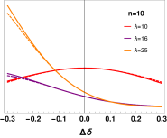
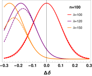
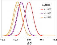
Figure 1: Exact and approximate Poisson likelihood of Eq. (27) (resp. plain and dashed curves) as a function of the nuisance parameter $\Delta\delta$.

We now plug the approximation Eq. (27) into the general likelihood $\bar{L}$, given in Eq. (20). The marginalisation of $\bar{L}$ is given by

$$\tilde{L}(\theta)=\int d\bar{\delta}\bar{L}(\theta,\bar{\delta})\bar{\pi}(\bar{\delta})\,,$$ (28)

where the combined prior $\bar{\pi}$ is given by Eq. (26) and involves the correlation matrix $\rho_{IJ}$ of the $\bar{\delta}$ given in Eq. (23). The approximate marginal likelihood is found to be

$$\tilde{L}(\theta)=L^{\rm stat}(\theta)L^{\rm sys}(\theta)=L^{\rm stat}(\theta)\,\frac{1}{\sqrt{|\eta\rho+1|}}\exp\left(\frac{1}{2}\xi\cdot\Big{(}\eta+\rho^{-1}\Big{)}^{-1}\cdot\xi\right)\,,$$ (29)

where “$\cdot$” is matrix multiplication, and one introduced the vector

$$\xi_{I}=\Delta_{I}\,(\hat{n}_{I}-\bar{n}_{0,I})\,,$$ (30)

the diagonal matrix $\eta$ with

$$\eta_{II}=(\Delta_{I})^{2}\,\bar{n}_{0,I}\,,$$ (31)

and $L^{\rm stat}=\prod_{I}{\rm Pr}(\hat{n}_{I}|\bar{n}_{0,I})$.

Both $\xi$ and $\eta$ depend on the parameters of interest $\theta$ via the expected event numbers and the combined uncertainties, i.e. one has in general $n_{0,I}(\theta)$, $\Delta_{I}(\theta)$. The $L^{\rm stat}$ term is almost the likelihood with no nuisance parameters, i.e. the piece of likelihood encoding the statistical uncertainty, except that it involves the shifted expected event numbers $\bar{n}_{0,I}$ (see Eq. (21)). In the limit of zero systematic uncertainty, i.e. $\Delta\rightarrow 0$, $L^{\rm sys}(\theta)$ becomes an irrelevant constant so that $\tilde{L}(\theta)\rightarrow L^{\rm stat}(\theta)$. The $L^{\rm sys}$ encodes most of the effect of the systematic uncertainties. Its effect is to enlarge and shift the preferred regions of the parameters of interest.

Frequentist marginalisation (i.e. profiling), as well as the Bayesian and frequentist bias methods described in [14] can all be treated analytically, substituting Eq. (28) by the appropriate operation. The approach described above and leading to Eq. (29) is general. Nevertheless it is interesting to work out specific cases that are omnipresent in LHC analyses.

3.1 Signal strength fit

The general approach summarised by Eq. (29) can be applied to the very typical case where the expected number of events is split into a signal and background component, $n=s+b$. The signal can be also further parametrised as $s=\mu s_{0}$, where the parameter of interest $\mu$ is a “signal strength modifier” and $s_{0}$ is some nominal value for the signal.

In principle both background and signal are plagued by systematic uncertainties, so that one should distinguish the elementary nuisance parameters for signal and background, $\delta^{s}$,$\delta^{b}$. After a preliminary step of error propagation, the systematic uncertainty on the expected rates take the form

$$\begin{split}n_{I}=&s_{I}\exp(\Delta^{s}_{1,I}\cdot\delta^{s}+(\delta^{s})^{t}\cdot\Delta^{s}_{2,I}\cdot\delta^{s})\\ &+b_{I}\exp(\Delta^{s}_{1,I}\cdot\delta^{b}+(\delta^{b})^{t}\cdot\Delta^{b}_{2,I}\cdot\delta^{b})\end{split}\,.$$ (32)

In order to obtain the standard form for propagated errors Eqs. (10), (11), (12) , one defines the overall vector of elementary uncertainties $\delta=(\delta^{s},\delta^{b})$, and write $n_{I}=n_{0,I}\exp(\Delta_{1,I}\cdot\delta+\delta^{t}\cdot\Delta_{2,I}\cdot\delta)$ where

$$n_{0,I}=s_{0,I}+b_{0,I}\,,\quad\Delta_{1,I}=\frac{(s_{0,I}\Delta^{s}_{1,I},\,b_{0,I}\Delta^{b}_{1,I})}{s_{0,I}+b_{0,I}}\,,$$ (33)

$$(\Delta_{2,I})_{ij}=\frac{1}{{s_{0,I}+b_{0,I}}}\begin{pmatrix}s_{0,I}(\Delta^{s}_{2,I}+(\Delta^{s}_{1,I})^{2}/2)&0\\ 0&b_{0,I}(\Delta^{b}_{2,I}+(\Delta^{b}_{1,I})^{2}/2)\end{pmatrix}-\frac{1}{2}(\Delta_{1,I})_{i}(\Delta_{1,I})_{j}\,.$$ (34)

This makes contact with the standard notation of Eq. (13), and the analytic marginal likelihood is readily given by Eq. (29). If the $N$ independent likelihoods correspond to $N$ measurements of a same process, one has $s_{0,I}=s_{0}$, $b_{0,I}=b_{0}$ for every $I$. This case will be illustrated in Sec. 4.

Here, positive $s$ and $b$ have been assumed. It is also possible to allow $s$ to take negative values if it is dominated by the destructive interference between the SM and BSM matrix elements. In that case a linear modelisation of the error on $s$ is fine, but one should bear in mind that if the support of the $\delta^{s}_{I}$ is such that $b+s$ can be zero, depending on the prior of $\delta^{s}_{I}$ the likelihood can blow up above some arbitrary large value of $s$. This is a general fact that is not specific to the approximations studied in this paper.

3.2 Differential distributions

Another typical measurement at the LHC is the one of a differential distribution. The likelihood with no systematic uncertainties has then the form of Eq. (14), where every measurement corresponds to a different bin $I$ , and $\hat{n}_{I}$ is the observed event number in the bin $I$. Denoting by $X\in\mathcal{D}$ the variable along which the events are binned and by $\mathcal{D}_{I}$ the subdomain of $\mathcal{D}$ defining the bin $I$, the expected event numbers are given by $n_{I}=n_{\rm tot}\int_{\mathcal{D}_{I}}dxf_{X}(x)$.

Differential distributions get deformed by detector effects, that typically smear their shape. A general way of modelling the smearing is to write the binning variable as

$$X=X_{0}(1+\Delta(X_{0})\delta)\,,$$ (35)

where $\Delta(X_{0})$ is the relative magnitude of the uncertainty at the location $X_{0}$. As a simple example, we assume a model of smearing independent of $X$ – the general case can be treated similarly. The expected number of events in a bin $I$ is given by

$$n_{I}=n_{\rm tot}\int_{\mathcal{D}_{I}}f_{X}(x(1+\Delta\delta))dx\,,$$ (36)

where $n_{\rm tot}$ is the expected total number of events. Starting from Eq. (14), one can disentangle the information of shape and total event number,

$$L(\theta,\delta)=L_{\rm tot}(\theta)L_{\rm shape}(\theta,\delta)\,,\quad L_{\rm shape}(\theta,\delta)=\prod_{I=1}^{n}\left(\frac{n_{I}(\theta,\delta)}{n_{\rm tot}(\theta)}\right)^{\hat{n}_{I}}\,.$$ (37)

Only $L_{\rm shape}$ depends on $\delta$, as this nuisance parameter models a shape deformation. Expanding $\log n$ over $\Delta$ at quadratic order gives

$$n_{I}=n_{I,0}\exp\left(\Delta_{1,I}\delta+\Delta_{2}{2,I}\delta\right)\,,$$ (38)

with

$$n_{I,0}=n_{\rm tot}\int_{\mathcal{D}_{I}}f_{X}(x)dx\,,\quad\Delta_{1,I}=\Delta\int_{\mathcal{D}_{I}}xf^{\prime}_{X}(x)dx\left(\int_{\mathcal{D}_{I}}f_{X}(x)dx\right)^{-1}\,,$$ (39)

$$\Delta_{2,I}=\frac{\Delta^{2}}{2}\left[\left(\int_{\mathcal{D}_{I}}x^{2}f^{\prime\prime}_{X}(x)dx\right)\left(\int_{\mathcal{D}_{I}}f_{X}(x)dx\right)^{-1}-\left(\int_{\mathcal{D}_{I}}xf^{\prime}_{X}(x)dx\right)^{2}\left(\int_{\mathcal{D}_{I}}f_{X}(x)dx\right)^{-2}\right]\,.$$ (40)

As an aside one may notice that when one expands $n_{I}$ at second order, the quadratic term explicitly shows the effect of smearing. If $f$ is convex (concave) over the bin, then $f_{X}^{\prime\prime}>0$ ($f_{X}^{\prime\prime}<0$), so that the quadratic term fills (depletes) the bin, accordingly to what is expected from a smearing process.

Plugging this expression into the likelihood gives exactly

$$L_{\rm shape}=L_{\rm shape}^{\rm stat}e^{\xi\delta-\eta\delta^{2}/2}\,,$$ (41)

with $\xi=\sum_{I}\Delta_{1,I}$, $\eta=2\sum_{I}\Delta_{2,I}$. Marginalising with a Gaussian prior for $\delta$ gives once again Eq. (29), here in a one-variable version:

$$\tilde{L}_{\rm shape}=L_{\rm shape}^{\rm stat}\frac{1}{\sqrt{\eta+1}}\exp\left(\frac{\xi^{2}}{2(\eta+1)}\right)\,.$$ (42)

Finally, the unbinned version of the same likelihood is directly obtained by taking the limit of infinitely thin bins. Then $\hat{n}_{I}$ can be only zero or one, the integrals can be simplified and the observed events end up labelled by their position $\hat{X}_{I}$. One gets

$$\Delta_{1,I}=\Delta\hat{X}_{I}\frac{f^{\prime}_{X}(\hat{X}_{I})}{f_{X}(\hat{X}_{I})}\,,\quad\Delta_{2,I}=\frac{\Delta^{2}}{2}(\hat{X}_{I})^{2}\left(\frac{f^{\prime\prime}_{X}(\hat{X}_{I})}{f_{X}(\hat{X}_{I})}-\frac{f^{\prime 2}_{X}(\hat{X}_{I})}{f^{2}_{X}(\hat{X}_{I})}\right)\,,$$ (43)

from which the marginal likelihood follows. The information that has to be reported to reconstruct this smeared likelihood is

• The magnitude of the relative uncertainty on the binning variable $X$,

• The first and second derivatives of the expected shape $f_{X}$.

4 An example of signal strength fit

Channel	A	B	C
$\hat{n}$	280	310	320
$\Delta^{s,1}$	$10\%$	$-10\%$	$10\%$
$\Delta^{s,2}$	$5\%$	$10\%$	$10\%$
$\Delta^{s,3}$	$0\%$	$-5\%$	$-5\%$
$\Delta^{b,1}$	$-10\%$	$-10\%$	$10\%$
$\Delta^{b,2}$	$5\%$	$10\%$	$-10\%$

Table 1: Observed data and nuisance parameters in three statistically independent channels $A,B,C$. The average expected background is taken to be $b_{0}=100$.

Figure 2: Likelihood functions drawn from data of Tab. 1. Plain line: Exact marginal likelihood, evaluated numerically. Dashed line: Approximate marginal likelihood, evaluated analytically. Dotted line: likelihood with no systematic uncertainties, $L^{\rm stat}(s)\equiv L(s,\delta=0)$.

In order to illustrate our results, we consider a somewhat realistic scenario for the characterisation of a signal. Formally, the scenario considered corresponds to a particular case of the signal strength analysis described in Sec. 3.1. This example will also be used to check the accuracy of the approximate marginal likelihood, $\tilde{L}$.

To carry out this toy analysis one first has to setup the “observed” data, the expected background and the systematic uncertainties. We assume three independent observation channels $I=(A,B,C)$. An observed event number $\hat{n}_{A,B,C}$ is assumed for each channel. The expected event number is given a signal+background form $n=s+b$, which is taken to be common to all channels, so that $s_{I}=s$, $b_{I}=b$, and the nominal value of $b$ is fixed.

We further assume the presence of 3 independent systematic uncertainties labelled $a,b,c$ for the signal and 2 uncertainties labelled $d,e$ for the background. Both signal and background are positive, so that we use the error modelisation of Eq. (5). We are going to consider cases of a flat and Gaussian prior for $\delta$, which imply respectively log-normal and log-flat priors for the $s$, $b$ components of the expected event number.

Assuming a first step of propagation from more elementary uncertainties, and disregarding the possible $\Delta_{2}$ terms for simplicity, the leading effect of the systematic uncertainties on the expected event number is characterised by $3\times 5$ numbers $\Delta_{1,I}^{s/b,i}$, given in Tab. 1. In the notation of Sec. 2.5, one has $N=3$, $p=5$. Note that with this starting point, the magnitude of the $p$ elementary uncertainties are already combined with the $N\times p$ derivatives of the expected signal. The uncertainties appear in each channel $I$ as $s=s_{0}\exp(\Delta^{s}_{1,I}.\delta^{s})$, $b=b_{0}\exp(\Delta^{b}_{1,I}.\delta^{b})$.

Having characterised the main effect of the systematic uncertainties, we can readily use the approximate marginal likelihood $\tilde{L}$. Moreover, we compute the exact marginal likelihood by numerically integrating over the five nuisance parameters, which provides a way of testing directly the accuracy of $\tilde{L}$. In practice, plotting the exact marginal likelihood of our example takes about an hour on a laptop with average specifications, while plotting the approximate likelihood is instantaneous.

All the numbers assumed for $\hat{n}_{I}$ and the $\Delta_{1,I}^{s/b,i}$ are given in Tab. 1. The observed numbers are chosen so that the statistical uncertainty be of $O(10\%)$. This is for example the case in the global fit of the 8 TeV Higgs signal strengths. The signs of the systematic uncertainties have been chosen so that the likelihood strongly depends on every nuisance parameter. The relative magnitudes of the elementary uncertainties are chosen to be $O(10\%)$.

This illustrative scenario can be used in order to check the accuracy of the two kinds of approximations required to obtain the $\tilde{L}$ likelihood: a) the CLT-based Gaussian approximation (see Sec. 2) and b) the likelihood expansion (see Sec. 3). The Gaussian and flat priors allow us to disentangle between these two approximations, because for Gaussian priors, approximation a) is always satisfied, i.e. the CLT is perfectly convergent. Thus for Gaussian priors, the discrepancies between the approximate and local likelihoods come only from approximation b). In contrast, in the flat prior case the discrepancies come from both approximations a) and b).

The exact and approximate marginal likelihoods are shown in Fig. 2. In the case of Gaussian priors for $\delta$ (i.e. log-normal uncertainties), the two curves agree very well. This shows that approximation b) is well under control. In order to test approximation a), i.e. the CLT convergence, we can now compare with the case of flat priors for $\delta$. It turns out that a mild discrepancy appears in certain regions. This illustrates the degree of convergence of the CLT in a five-parameters case. The two curves agree still fairly well in this flat-prior case, in the sense that the best-fit regions drawn from these likelihoods would be similar. For a larger number of nuisance parameters, this discrepancy is expected to decrease as the CLT convergence should improve.

5 Conclusion

With the goal of simplifying the treatment of systematic uncertainties in typical LHC analyses, we have studied the behaviour of a generic likelihood in the presence of a large number of uncertainties with small relative magnitudes.

Whenever this condition is satisfied, it turns out that well-controled approximations become available, which provide a way of drastically simplifying the incorporation of systematic uncertainties into the likelihood. Our demonstration is split into steps of error propagation and error combination. In the latter, the Lyapunov central limit theorem applies to the combined uncertainties, thereby approximating their joint distribution as a multivariate normal. This implies that the shape of the priors of the elementary uncertainties is irrelevant – only their magnitudes matter.

Whenever the combined uncertainties are small enough, say $\lesssim 20\%$, the likelihood can be further simplified and the complete marginal likelihood is obtained analytically. This general result is applied to the important cases of signal strength characterisation and differential distribution smearing.

For illustration, we present a toy-analysis of signal strength characterisation including systematic uncertainties on signal and background. The approximate and exact marginal likelihoods are found to be in fairly good agreement in this example, implying that all approximations are well under control.

Beyond the obvious gain of avoiding heavy numerical marginalisation, another practical matter is the communication of systematic uncertainties, for example from an experiment to the public. Our approach implies that all the needed information is encoded into a finite set of numbers, namely the relative magnitude of elementary uncertainties and the derivatives of the expected event numbers. The transmission of this information is straightforward, and gives a fairly human-readable summary of the systematic uncertainties. In principle, this simple method could be used to make public the detector effects that are included in LHC analyses.

The marginal likelihood presented in this paper is purely Bayesian. It is also possible to compute analytically the marginal likelihood in case of a frequentist profiling (described in App. A), as well as to apply the bias methods formalised in Ref. [14]. Finally, although our study is oriented towards LHC analyses, it could also be readily applied into other experimental contexts.

Appendix A Analytic frequentist marginalisation

In Sec. 3, a frequentist marginalisation of the combined uncertainties can also be done. This is obtained by substituting Eq. (28) with

$$\tilde{L}(\theta){\rm freq}=\max_{\bar{\delta}}\left[\bar{L}(\theta,\bar{\delta})\bar{\pi}(\bar{\delta})\right]\,.$$ (44)

The resulting approximate likelihood is

$$\tilde{L}(\theta){\rm freq}=L^{\rm stat}(\theta)\,\exp\left(\frac{1}{2}\xi\cdot\Big{(}\eta+\rho^{-1}\Big{)}^{-1}\cdot\xi\right)\,,$$ (45)

which ressembles very much the Bayesian result up to a $\sqrt{|\eta\rho+1|}$ factor. Typically, the variation of this factor with respect to the parameters of interest is small compared to the variation of the exponential term. Hence, in practice, the frequentist and Bayesian approximate likelihoods are almost equivalent. The subsequent frequentist and Bayesian best-fit regions obtained from these likelihoods thus differ mostly by the definition of frequentist and Bayesian contours [15].

References

- [1] W. Verkerke and D. P. Kirkby, “The RooFit toolkit for data modeling,” eConf C 0303241, MOLT007 (2003) [physics/0306116].
- [2] L. Moneta et al., “The RooStats Project,” PoS ACAT 2010, 057 (2010) [arXiv:1009.1003 [physics.data-an]].
- [3] S. Kraml et al., “Searches for New Physics: Les Houches Recommendations for the Presentation of LHC Results,” Eur. Phys. J. C 72, 1976 (2012) [arXiv:1203.2489 [hep-ph]].
- [4] F. Boudjema et al., “On the presentation of the LHC Higgs Results,” arXiv:1307.5865 [hep-ph].
- [5] K. Cranmer, S. Kreiss, D. Lopez-Val and T. Plehn, Phys. Rev. D 91, no. 5, 054032 (2015) [arXiv:1401.0080 [hep-ph]].
- [6] A.C. Berry, “The Accuracy of the Gaussian Approximation to the Sum of Independent Variates,” Transactions of the American Mathematical Society 49.1,122–136 (1941): .
- [7] C.G. Esseen, “On the Liapunoff limit of error in the theory of probability,” Ark. Mat. Astr. Fys, A28, n.9, 1-19, (1942)
- [8] W. Feller, An Introduction to Probability Theory and Its Applications, Vol. 2, 3rd ed. New York: Wiley, 257–258, (1971).
- [9] S. Fichet, G. von Gersdorff, “Effective theory for neutral resonances and a statistical dissection of the ATLAS diboson excess,” JHEP 1512, 089 (2015) [arXiv:1508.04814 [hep-ph]].
- [10] G. Aad et al. [ATLAS Collaboration], “Search for high-mass diboson resonances with boson-tagged jets in proton-proton collisions at TeV with the ATLAS detector,” JHEP 1512, 055 (2015) [arXiv:1506.00962 [hep-ex]].
- [11] A. Arbey, S. Fichet, F. Mahmoudi, G. Moreau “The correlation matrix of Higgs rates at the LHC,” arXiv:1606.00455 [hep-ph].
- [12] P. Billingsley, Probability and measure (1995), 2nd edition, John Wiley and Sons, Inc.,New York, 186
- [13] J. W.Lindeberg , “Über den zentralen Grenzwertsatz der Wahrscheinlichkeitsrechnung, II,” Math. Zeit., 15,1, 211–225, 1922.
- [14] S. Fichet and G. Moreau, “Anatomy of the Higgs fits: a first guide to statistical treatments of the theoretical uncertainties,” arXiv:1509.00472 [hep-ph].
- [15] K. A. Olive et al. [Particle Data Group Collaboration], “Review of Particle Physics,” Chin. Phys. C 38, 090001 (2014).