Deuterium target data for precision neutrino-nucleus cross sections
Abstract
Amplitudes derived from scattering data on elementary targets are basic inputs to neutrino-nucleus cross section predictions. A prominent example is the isovector axial nucleon form factor, , which controls charged current signal processes at accelerator-based neutrino oscillation experiments. Previous extractions of from neutrino-deuteron scattering data rely on a dipole shape assumption that introduces an unquantified error. A new analysis of world data for neutrino-deuteron scattering is performed using a model-independent, and systematically improvable, representation of . A complete error budget for the nucleon isovector axial radius leads to , with a much larger uncertainty than determined in the original analyses. The quasielastic neutrino-neutron cross section is determined as . The propagation of nucleon-level constraints and uncertainties to nuclear cross sections is illustrated using MINERvA data and the GENIE event generator. These techniques can be readily extended to other amplitudes and processes.
pacs:
13.15.+g 14.60.Pq 14.20.DhI Introduction
Current and next generation accelerator-based neutrino experiments are poised to answer fundamental questions about neutrinos Acciarri:2015uup ; Itow:2001ee ; Adamson:2016tbq ; Adamson:2016xxw ; Chen:2007ae . Precise neutrino scattering cross sections on target nuclei are critical to the success of these experiments. These cross sections are computed using nucleon-level amplitudes combined with nuclear models. Determination of the requisite nuclear corrections presently relies on data-driven modeling Andreopoulos:2009rq ; Hayato:2009zz ; Buss:2011mx ; Golan:2012wx employing experimental constraints Drakoulakos:2004gn ; AguilarArevalo:2010zc ; AguilarArevalo:2010bm ; AguilarArevalo:2010cx ; Abe:2015awa ; Anderson:2011ce ; Rodrigues:2015hik ; Megias:2016lke . Ab initio nuclear computations are beginning to provide additional insight Lovato:2013cua ; Bacca:2014tla ; Carlson:2014vla . Regardless of whether nuclear corrections are constrained experimentally or derived from first principles, independent knowledge of the elementary nucleon-level amplitudes is essential. In this paper, we address the problem of model-independent extraction of elementary amplitudes from scattering data, and the propagation of rigorous uncertainties through to nuclear observables.
The axial-vector nucleon form factor, , is a prominent source of uncertainty in any neutrino cross section program. While the techniques employed in the present paper may be similarly applied to other elementary amplitudes, such as vector form factors vector , we focus on the axial-vector form factor, which is not probed directly in electron scattering measurements, and which has large uncertainty.
The axial form factor is constrained, with a varying degree of model dependence, by neutron beta decay Agashe:2014kda , neutrino scattering on nuclear targets heavier than deuterium Lyubushkin:2008pe ; AguilarArevalo:2010zc ; Brunner:1989kw ; Pohl:1979zm ; Auerbach:2002iy ; Belikov:1983kg ; Bonetti:1977cs , pion electroproduction Bernard:2001rs and muon capture Andreev:2012fj . Existing data for the neutrino-deuteron scattering process provide the most direct access to the shape of the axial-vector nucleon form factor. The assumption of a neutron at rest and barely bound in the laboratory frame permits unambiguous energy reconstruction, eliminating flux uncertainties. The abundant neutrino scattering data on heavier targets involve degenerate uncertainties from neutrino flux, and from large and model-dependent nuclear corrections, complicating the extraction of nucleon-level amplitudes. Antineutrino scattering on hydrogen would entirely eliminate even the nuclear corrections required for deuterium, but there are no high-statistics data for this process. Given the importance of deuterium data for the axial form factor, it is imperative to quantify the constraints from existing data.
In this paper, we present the charged-current axial-vector nucleon form factor and error budget determined from neutrino-deuterium scattering data. In place of the dipole assumption (cf. Eq. (9) below) used in previous analyses of the form factor, we employ the model-independent expansion111Formalism for expansion and nucleon form factors is described in Refs. Bhattacharya:2011ah ; Hill:2010yb , and several applications are found in Refs. Lorenz:2014vha ; Epstein:2014zua ; Lee:2015jqa ; Bhattacharya:2015mpa . Related formalism and applications may be found in Hill:2006ub ; Bourrely:1980gp ; Boyd:1994tt ; Boyd:1995sq ; Lellouch:1995yv ; Caprini:1997mu ; Arnesen:2005ez ; Becher:2005bg ; Hill:2006bq ; Bourrely:2008za ; Bharucha:2010im ; Amhis:2014hma ; Bouchard:2013pna ; Bailey:2015dka ; Horgan:2013hoa ; Lattice:2015tia ; Detmold:2015aaa . parametrization. The resulting uncertainty is significantly larger than found in previous analyses Bodek:2008epjc ; Kuzmin:2007kr ; Bernard:2001rs of the deuterium constraint on the axial form factor using multiple data sets. This larger uncertainty results from removing the dipole assumption, and from including systematic errors for experimental acceptance corrections and for model-dependent deuteron corrections. The new constraints may be readily implemented in nuclear models and neutrino event generators.
The remainder of the paper is structured as follows. In Sec. II we introduce the deuterium data sets and perform fits to the dipole model for the axial form factor. This is done in order to compare with original publications, and to isolate the impact of form factor shape assumptions versus other inputs or data selections. In Sec. III we review the relevant expansion formalism, and redo fits from Sec. II replacing dipole with expansion. Several features of these fits indicate potentially underestimated systematic errors in corrections that were applied to data in the original publications. Section IV describes a range of systematics tests. We consider several sources of systematic errors in more detail in Sec. V, and redo fits in Sec. VI, where we present final results for . In Sec. VII we illustrate the propagation of errors to several derived observables, including the isovector axial nucleon radius and total neutrino-nucleon quasielastic cross sections. The incorporation of nucleon-level uncertainties in nuclear cross sections is illustrated with MINERvA data Fiorentini:2013ezn . Section VIII provides a summary and conclusion.
II Deuterium data and dipole fits
| Input | BNL1981 | ANL1982 | FNAL1983 | This work | Reference |
|---|---|---|---|---|---|
| -1.23 | -1.23 | -1.23 | -1.2723 | Agashe:2014kda | |
| 3.708 | 3.71 | 3.708 | 3.7058 | Agashe:2014kda | |
| Olsson Olsson:1978dw | Olsson Olsson:1978dw | Olsson Olsson:1978dw | BBA2005 | Bradford:2006yz | |
| PCAC | PCAC | PCAC | PCAC | (1) | |
| Deuteron correction | Singh Singh:1971md | Singh Singh:1971md | Singh Singh:1971md | Singh | Singh:1971md |
| lepton mass | except ABC | except ABC | |||
| range | |||||
| 49 | 49 | 30 | |||
| 1236 | 1792 | 354 | |||
| kinematic cut |
The world data from deuterium bubble chamber experiments consists of deuterium fills of the ANL 12-foot deuterium bubble chamber experiment Mann:1973pr ; Barish:1977qk ; Miller:1982qi , the BNL 7-foot deuterium bubble chamber experiment Baker:1981su , and the FNAL 15-foot deuterium bubble chamber experiment Kitagaki:1983px . We refer below to these experiments as ANL1982, BNL1981 and FNAL1983, respectively.222 An updated BNL data set was presented in Ref. Kitagaki:1990vs with a factor increase in number of events. However, we were unable to extract a sufficiently precise distribution of events from this reference, since the data were presented on a logarithmic scale (cf. Ref. Kitagaki:1990vs , Fig. 5). We thus consider only the events from the BNL1981 data set.
II.1 Fits to distributions
Extracting the axial form factor from data requires information about all other aspects of the scattering cross-section. The original publications used a variety of different inputs for axial () and magnetic () couplings, vector and pseudoscalar form factors, nuclear corrections, and muon mass corrections. Table 1 displays the input choices made in the original publications for each of the three considered data sets, as well as the updated inputs used for the remainder of this paper.333 Form factor notations and conventions are as in Ref. Bhattacharya:2011ah .
The vector form factors are constrained by invoking isospin symmetry and constraints of electron-nucleon scattering data. In place of the Olsson vector form factors Olsson:1978dw , we use the so-called BBA2005 parametrization that is commonly employed in contemporary neutrino studies Bradford:2006yz . Similar results were obtained using the BBA2003 Budd:2003wb and BBBA2007 Bodek:2007ym parametrizations. Recent developments, connected with the so-called “proton radius puzzle”, point to potential shortcomings in previous extractions of the vector form factors Pohl:2010zza ; Bernauer:2013tpr ; Lee:2015jqa . A systematic study of the vector form factors similar to the expansion analysis of the axial form factor presented here is undertaken in Refs. Lee:2015jqa ; vector .
For the pseudoscalar form factor , we employ the partially conserved axial current (PCAC) ansatz,
| (1) |
The free-nucleon form factors and are functions of the four momentum transfer from the lepton to the nucleon, and , are the masses of the nucleon and the pion. The effects of the pseudoscalar form factor are suppressed in the limit of small lepton mass, and its uncertainties are negligible in most applications involving accelerator neutrino beams, including this analysis.
Nuclear corrections relating the free neutron cross section, , to the deuteron cross section, , may be parametrized as
| (2) |
where denotes the deuteron differential cross section with respect to the intrinsically positive = .444 For definiteness in the deuteron case, we let in Eq. (2) denote the leptonic momentum transfer. This definition is consistent with the experimental reconstruction, which assumed the kinematics for scattering from a free neutron in the presence of a spectator proton carrying opposite momentum to the neutron. The model of Ref. Singh:1971md was used in the original analyses, with independent of neutrino energy, and above . We retain this model as default, but examine deviations from this simple description below in Sec. IV, using the calculations of Ref. Shen:2012xz .
The neutrino-neutron quasielastic cross section may be written in a standard form
| (3) |
where is the difference of Mandelstam variables, , and are quadratic functions of nucleon form factors LlewellynSmith:1971zm , and the vector-axial interference term changes sign for the scattering process. In the BNL1981 and FNAL1983 data sets, the lepton mass was neglected inside the functions , and of Eq. (3), but retained in other kinematic prefactors. In our analysis, we retain the complete lepton mass dependence.
The event distributions in have been obtained by digitizing the relevant plots from the original publications. Table 1 gives the range and bin size, the total number of events,555 For BNL1981 and ANL1982, the digitized number of events in each bin was rounded to the nearest integer, resulting in the same total numbers, 1236 and 1792 respectively, quoted in the original publications. For FNAL1983, the digitization produced near-integer results in each bin, but the total summed event number, 354, differs from the value 362 quoted in the original publication. and the minimum retained in the original analyses. In each case, events in a lowest bin were omitted from fits, and only FNAL1983 reports these events. We retain the same binning and minimum cut in our default fits. These distributions are included as Supplemental Material to the present paper self .
II.2 distributions and flux
An advantage of the process in an exquisite device like a bubble chamber is the accurate reconstruction of the neutrino energy for each event. Cross section parameters can be constrained from the distribution despite poorly controlled uncertainties in ab initio neutrino flux estimates. This is especially valuable for the low energy ANL1982 and BNL1981 data, whose neutrino energy spectrum significantly influences the shape of the distribution through the energy-dependent kinematic limit corresponding to a backscattered lepton.
Unfortunately, event-level kinematics from the deuterium data sets are no longer available and unbinned likelihood fits using the and dependence of the cross section cannot be repeated. However, the one-dimensional distribution of events in reconstructed neutrino energy, , may be extracted from the original publications, and we use this information to reconstruct the flux self-consistently. This subsection describes the procedure we use, including some subtle points required for later interpretation of the form factor fits.
The differential neutrino flux is determined by
| (4) |
where is the free-neutron quasielastic cross section, and is the energy distribution of free-neutron events that would be obtained in the experimental flux. The constant of proportionality in Eq. (4) is determined by the number of target deuterons and the time duration of the experiment. Let us normalize the energy distribution according to
| (5) |
Consistency in Eq. (5) is obtained when , where
| (6) |
The right-hand side of Eq. (6) may be computed using a given , and depends on and through Eqs. (2) and (4). Using the flux from Eq. (4), we have finally,
| (7) |
where a fit parameter, , has been introduced for the normalization.
Choosing in Eq. (5) would correspond to . In order to avoid the explicit computation of the integrals (6), we instead take , corresponding to the expectation . We allow the parameter to float unconstrained in the fits, with an independent parameter for each experiment.
We emphasize that in Eq. (4) represents the energy distribution of free-neutron events that would be obtained in the experimental flux; this distribution is obtained from the energy distribution of observed events in deuterium by correcting for nuclear effects, for events lost due to the cut, and for other experimental effects. Such corrections were applied to the energy distribution presented in the BNL1981 data set, but not in the ANL1982 and FNAL1983 data sets. The effect of applying or not applying these corrections is found to be small, as discussed below in Sec. V.1.
For later comparison, we compute the ratios (6) with a nominal dipole axial form factor (, cf. Eq. (9) below), neglecting deuteron corrections (), and at a nominal neutrino energy, for the values employed in the BNL1981, ANL1982, FNAL1983 data sets:666 While is close to the peak energy for the BNL1981 and ANL1982 data sets, the FNAL1983 data set involved higher energy. However, these ratios have mild energy dependence above , e.g. at the result is .
| (8) |
We expect these numbers to be approximately reproduced in when the deviation from in Eq. (6) is dominated by the cut.
Two further complications result in technical subtlety but do not affect the fit results. First, the binned event rate for ANL1982 is provided in a prior publication Barish:1978pj that used a subset of about half the events. A second complication is the finite bin width of the distributions, which would yield unphysical discontinuities when displaying ANL and BNL spectra at best fit. This effect is the result of convoluting a low energy flux with a differential cross section that has an energy-dependent kinematic limit. We use an interpolation algorithm to produce smoothed fluxes with 500 bins in energy over the original range of data. Nearly identical fit results are obtained regardless of whether the interpolation is a cubic spline, linear, or whether the original binning is used, so this step is primarily cosmetic. The smoothed and unsmoothed distributions are included as Supplemental Material to the present paper self .
II.3 Dipole fits
| BNL 1981 Baker:1981su | 1.07(6) | 1.07(5) | 1.05(5) |
|---|---|---|---|
| ANL 1982 Miller:1982qi | 1.05(5) | 1.05(5) | 1.02(5) |
| FNAL 1983 Kitagaki:1983px | 1.20(11) | 1.17(10) |
Our results for the axial form factor will differ from the analyses in the original publications. These differences arise from a number of sources: updated numerical inputs in Table 1; not using unbinned likelihood fits; and differences in axial form factor shape assumptions. In order to understand these differences, we begin by restricting attention to the dipole ansatz,
| (9) |
and compare to fits in the original publications.
Table 2 gives results for fits to the dipole ansatz (9) for the axial form factor. The table shows “flux-independent” results from the original experiments, which performed unbinned likelihood fits to event-level data. Our results are from a Poisson likelihood fit to the binned distribution of events obtained with a neutrino flux given by smoothing the binned reconstructed neutrino energy distribution (divided by theoretical cross section), as described in Sec. II.2. Fits to the binned log-likelihood function are found by minimizing the function
| (10) |
where is the number of events in the th bin, and is the theory prediction (7) for the bin. Errors correspond to changes of in the LL function.
Because we do not use an unbinned likelihood fit, we do not expect precise agreement even when the original choices of constants in Table 1 are used. Comparing the first two columns of Table 2, the size of the resulting statistical uncertainties are approximately equal, and only FNAL shows a discrepancy in central value. A similar exercise was performed in Refs. Budd:2003wb ; Bodek:2003ed ; Budd:2004bp , and similar results were obtained. Having reproduced the original analyses to the extent possible, we will proceed with the updated constants as in the final column of Table 1.
III expansion analysis
The dipole assumption (9) on the axial form factor shape represents an unquantified systematic error. We now remove this assumption, enforcing only the known analytic structure that the form factor inherits from QCD. We investigate the constraints from deuterium data in this more general framework. A similar analysis may be performed using future lattice QCD calculations in place of deuterium data.
III.1 expansion formalism
The axial form factor obeys the dispersion relation,
| (11) |
where represents the leading three-pion threshold for states that can be produced by the axial current. The presence of singularities along the positive real axis implies that a simple Taylor expansion of the form factor in the variable does not converge for . Consider the new variable obtained by mapping the domain of analyticity onto the unit circle Bhattacharya:2011ah ,
| (12) |
where , with , is an arbitrary number that may be chosen for convenience. In terms of the new variable we may write a convergent expansion,
| (13) |
where the expansion coefficients are dimensionless numbers encoding nucleon structure information.
| 1.0 | 0 | 0.44 |
| 3.0 | 0 | 0.62 |
| 1.0 | 0.23 | |
| 3.0 | 0.45 | |
| 3.0 | 0.35 |
In any given experiment, the finite range of implies a maximal range for that is less than unity. We denote by the choice which minimizes the maximum size of in the range . Explicitly,
| (14) |
Table 3 displays for several choices of and .
The choice of can be optimized for various applications. We have in mind applications with data concentrated below , and therefore take as default choice,
| (15) |
minimizing the number of parameters that are necessary to describe data in this region. Inspection of Table 3 shows that the form factor expressed as becomes approximately linear. For example, taking implies that quadratic, cubic, and quartic terms enter at the level of , and .
The asymptotic scaling prediction from perturbative QCD Lepage:1980fj , , implies the series of four sum rules Lee:2015jqa
| (16) |
We enforce the sum rules (16) on the coefficients, ensuring that the form factor falls smoothly to zero at large . Together with the constraint, this leaves free parameters in Eq. (13). From Eq. (16), it can be shown Lee:2015jqa that the coefficients behave as at large . We remark that the dipole ansatz (9) implies the coefficient scaling law at large , in conflict with perturbative QCD.
In addition to the sum rules, an examination of explicit spectral functions and scattering data Bhattacharya:2011ah motivates the bound of
| (17) |
As noted above, from Eq. (16), the coefficients behave as at large . We invoke a falloff of the coefficients at higher order in ,
| (18) |
The bounds are enforced with a Gaussian penalty on the coefficients entering the fit. We investigate fits using a range of , other choices of , and alternatives to Eqs. (17) and (18), which are briefly reported in Sec. IV.
III.2 expansion basic fit results
| Dipole | |||||||||||||
|---|---|---|---|---|---|---|---|---|---|---|---|---|---|
| Experiment | LL | LL | LL | LL | |||||||||
| BNL1981 | 70.9 | 76.1 | 73.4 | 71.0 | 49 | ||||||||
| ANL1982 | 58.6 | 62.3 | 60.9 | 59.9 | 49 | ||||||||
| FNAL1983 | 38.2 | 39.1 | 39.1 | 39.1 | 29 |
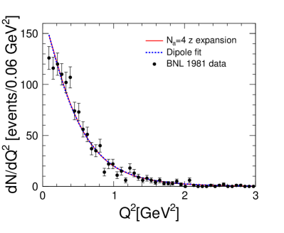

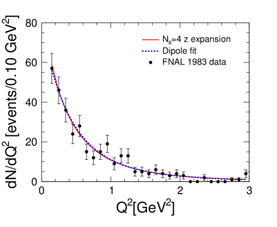
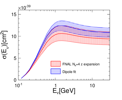
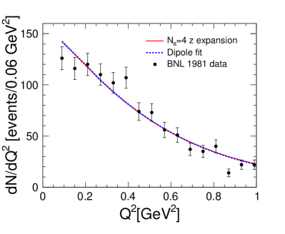
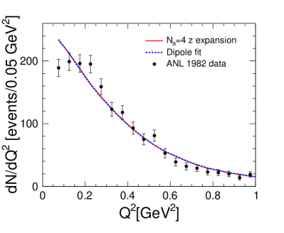
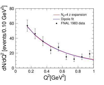
Using the same data sets and constants as described in Sec. II and summarized in Table 1, we perform fits replacing dipole axial form factor with expansion as in Eq. (13). We use the scheme choice (15), enforce the sum rule constraints (16), and use the default bounds on the coefficients in Eqs. (17), (18). The results are summarized in Table 4 and displayed in Figs. 1 and 2. The coefficients corresponding to the fits with free parameters in Table 4 are
| (22) |
where (symmetrized) errors correspond to a change of 1.0 in the LL function.
Table 4 summarizes expansion fits with different numbers of free parameters. Focusing on the first order coefficient,
| (26) |
As discussed after Eq. (15), , , , etc., terms in the expansion become increasingly irrelevant, corresponding to in Table 3. This is borne out by the data, which determines a form factor with coefficients in Eq. (III.2) of order 1.0 that mostly do not push the Gaussian bounds, and a leading coefficient in Eq. (III.2) that is approximately the same regardless of whether terms beyond order are included.
The axial “charge” radius is defined via the form factor slope at ,
| (27) |
For a general scheme choice , this quantity depends on all the coefficients in the expansion. Table 4 illustrates that is poorly constrained without the restrictive dipole assumption. We will provide a final value for the axial radius from deuterium data after discussion of systematic errors in the next section.
The normalization factor is also included in Table 4. This parameter is allowed to float without bounds, but returns values consistent with the approximation (II.2) to the expectation (6).
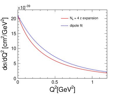
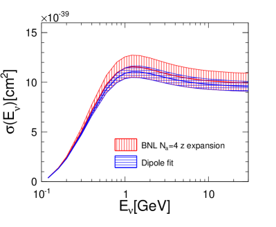
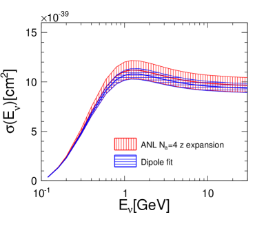
An interesting feature of the fits displayed in Fig. 1 is that whereas the best-fit curves for dipole and expansion are very similar in the considered range, derived observables such as the radius in Table 4, and the absolutely normalized cross section in Fig. 2, can be markedly different. The presence of the cut, and the lack of an absolutely normalized flux, explains this situation, which is most apparent for FNAL1983. To illustrate, Fig. 3 shows the absolutely normalized computed using the central value dipole and -expansion axial form factors for FNAL1983 in Figs. 1 and 2. Omitting the lowest- data, and applying an overall normalization factor obscures the difference between these curves.
The normalization parameter appearing in Eq. (7) is not externally constrained in our shape fits. The uncertainty after fitting yields for BNL1981 and ANL1982 and for FNAL1983, which is significantly larger than the to uncertainty from Poisson statistics. A simple Poisson constraint would not be adequate considering uncertainties from acceptance and deuterium corrections described later. A rate+shape fit with a correctly motivated uncertainty on could in principle produce a somewhat better constrained form factor and cross section.
III.3 Residuals analysis
The best fits are still a relatively poor description of the data, apparent in both Table 4 and Fig. 1. This was briefly discussed in the thesis Miller:1981thesis that accompanies the ANL1982 publication: the theoretical curve is too high at very low , becoming too low above 0.2 GeV2, and too high again around 0.7 GeV2. Similarly, the BNL1981 publication discusses the possibility of residual scanning biases with a kinematic dependence that mimics evidence for second-class currents violating the symmetries of QCD (cf. Ref. Baker:1981su , Fig. 5). These observations motivate a careful examination of systematic uncertainties assigned in the fits.
The preference of the experiments for a common -dependent distortion can be illustrated by comparing the residual discrepancy between the data and the best fit curves from Fig. 1 in a single plot, shown in Fig. 4.777 For definiteness, the best fit curve is from a simultaneous fit to the BNL, ANL and FNAL data sets. A nearly identical plot is obtained if different best fit curves for each data set are used.
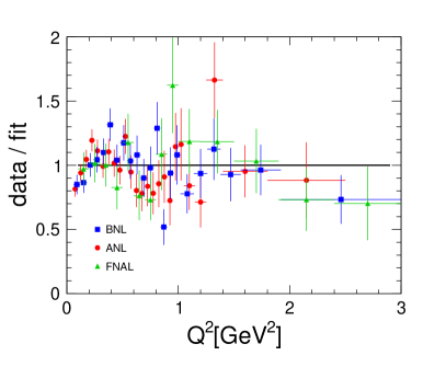
The distortion at lowest is clearly significant. The data also seem to agree on potential distortions in the range . However the null hypothesis, that the data in this range were drawn from a flat distribution, yields P-value of 0.12 and is not exceptional. In order to use a fit for this P-value and to improve the plot readability, the upper bins in each data set were combined.
Form factors described by the expansion, hence any form factor consistent with QCD, cannot accommodate such localized distortions of the spectrum (the dipole ansatz similarly cannot accommodate such distortions). The model for deuterium used by the original experiments asymptotically approaches unity and also does not cause such distortions. It is interesting to consider whether more complete deuteron correction models, such as Ref. Shen:2012xz (considered below in Fig. 6), could produce such distortions.888 Calculations of multinucleon effects for heavier nuclei like carbon exhibit qualitatively similar characteristics throughout this region of Martini:2009uj ; Gran:2013kda . Finally, the impact of residual scanning biases should also be accounted for. In the next sections we turn to the question of assigning a systematic uncertainty to account for such effects.
IV Systematic tests
Fits using different choices for constructing the expansion form factors should yield equivalent results for physical observables: a dependence on such choices would indicate an underestimated systematic uncertainty. Similarly, fits using different ranges of should yield equivalent results.
IV.1 Form factor scheme dependence
A test with variations of the number of free parameters was presented in Eq. (III.2) of the previous section. In order to translate other test fits into parameters that can be compared side-by-side, we will consider in all cases the dimensionless shape parameter defined by
| (28) |
where , as in Eq. (15). To motivate the choice (28), note that since is a small parameter, the form factor is approximately linear when expressed as a function of . The slope of this approximately linear function is the essential shape parameter determined by the data, and for convenience we define the slope at . [The axial radius is similarly defined as the form factor slope at in Eq. (27).]
IV.1.1 Magnitude of bound
IV.1.2 Choice of
Next, consider the choice of .999For , by design, the shape parameter is identified with the linear coefficient of the expansion in Eq. (13). Since [Eq. (28)] is a physical observable, it can be computed for any choice of . A different choice of requires more parameters to achieve the same truncation error, . We compare the default case of and to the case of and ,101010 Both cases have in the range . finding
| (37) |
where the errors are propagated using the covariance matrix for the coefficients . Nearly identical results are obtained for different choices of .
IV.2 Subsets of the range
A nonstatistical scatter of data points about the best fit curves is apparent in Fig. 1, and indicated by the poor fit quality in Table 4. Removing subsets of the data at high or low will help isolate sources of tension between data and fit.
| Dipole | |||||||||||||
|---|---|---|---|---|---|---|---|---|---|---|---|---|---|
| Experiment | LL | LL | LL | LL | |||||||||
| BNL1981 | 24.7 | 27.2 | 27.0 | 26.6 | 16 | ||||||||
| ANL1982 | 28.2 | 31.7 | 30.5 | 29.2 | 19 | ||||||||
| FNAL1983 | 8.3 | 8.3 | 8.2 | 8.1 | 9 |
| Dipole | |||||||||||||
|---|---|---|---|---|---|---|---|---|---|---|---|---|---|
| Experiment | LL | LL | LL | LL | |||||||||
| BNL1981 | 60.7 | 62.4 | 61.5 | 60.9 | 47 | ||||||||
| ANL1982 | 43.2 | 45.8 | 45.8 | 45.8 | 46 | ||||||||
| FNAL1983 | 38.2 | 39.1 | 39.1 | 39.0 | 28 |
First, consider the removal of high data, fitting to bins whose center is within the restricted range . The analog of Table 4 for this case is given by Table 5. Figure 5 shows comparisons of best fit curves and data points. The analog of Eq.(III.2) is
| (41) |
The omission of low- data has a similarly large effect on the fit parameters. Fitting to the range , the results are given in Table 6. The expansion coefficients are determined for to be
| (45) |
Comparing the results in Tables 4, 5, and 6 and in Eqs. (III.2), (IV.2), and (IV.2), we see that the leading and parameters shift in some cases by about twice the statistical uncertainty of the fits. This reflects how different parts of the range contribute to tensions in the fit. The minimum value of decreases in both cases, closer to a range that would be considered an adequate description of the data. The improvement when eliminating the low- region is especially striking considering it amounts to only two or three bins of data in each data set.
One method to translate the tensions in the fit to an uncertainty on the fit parameters is to consider what additional error is necessary to obtain a reduced of unity. We include an error for each data point proportional to the number of events in the original distribution. This requires the use of a calculation instead of a log-likelihood fit, which we achieve by limiting the test to the sample with . Adding this error in quadrature to the statistical error, we see that for BNL, an additional error is required, while ANL requires an additional error.
V Systematic errors
The experimental uncertainties in the fits summarized in Table 4 correspond only to statistical errors on the number of events in each bin. With a framework in place to quantify theoretical form factor shape uncertainty, let us examine several sources of systematic error, and their impact on the extraction of .
Experimental systematic uncertainties come from the construction of the neutrino flux, and from acceptance corrections. A theoretical systematic error arises from uncertain modeling of deuteron effects.
V.1 Flux
Our procedure includes a self-consistent determination of the neutrino flux for fits to the distributions, as described in Sec. II.2. Systematic uncertainty estimates in the experimenter’s ab initio flux do not apply. Instead we check for sensitivity to fluctuations in the number of events by varying one bin by its statistical error, reextracting fit parameters, and then repeating for all bins. Adding errors in quadrature, the result for the BNL data set is
| (46) |
Such an additional flux error is numerically subleading compared to statistical error, and also to the systematic error assigned below to account for deuteron and acceptance corrections. We neglect it in our final fits.
The consistency of the flux procedure could also be impacted by distortions of the distribution by cuts or deuteron corrections. Recall that the energy distribution from BNL1981, but not from ANL1982 or FNAL1983, was corrected for these effects. We have checked that the resulting variations are even smaller than the statistical fluctuations in Eq. (46), and are neglected.
V.2 Acceptance corrections
One source of uncertainty, especially in the limit of very low , is the acceptance corrections associated with human-eye scanning of the bubble chamber photographs. For example, Fig. 1 of ANL 1982 Miller:1982qi provides an estimate of the scanning efficiency ranging from at to for . We include a possible correlated efficiency correction by making the following replacement in the efficiency-corrected number of events:
| (47) |
Here is a parameter introduced in the fit, and we use a simple linear interpolation of the function in Ref. Miller:1982qi for the efficiency and efficiency error .
In the BNL data set, an efficiency effect with similar magnitude is presented, but not directly in the variable. For simplicity we take the ANL function to represent possible effects also in the BNL and FNAL data sets, with independent floating scale parameters in Eq. (47). The shape parameters and minimum values are as follows, comparing results with and without the acceptance correction,
| (50) | ||||
| (53) | ||||
| (56) |
The parameter takes on values of , , and for data from ANL1982, BNL1981, and FNAL1983 respectively; the negative values indicate a pull to decrease the predicted cross section to match the data. In each case there is only modest improvement in the fit quality, and small impact on the form factor shape. Acceptance corrections within the quoted range have only minor impact.
V.3 Deuteron corrections
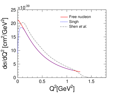
The analysis to this point, like the original analyses, used the deuteron correction model of Singh Singh:1971md . This model yields a suppression of the cross section for GeV2.111111 A follow-up analysis Singh:1986xh considers effects of meson exchange currents and alternate deuteron wave functions, with a total result very similar to Ref. Singh:1971md . An example of a modern calculation with extended range in energy and is given by Shen et al. in Ref. Shen:2012xz .121212See also Ref. Moreno:2015nsa . The Shen et al. model is overlaid with the original Singh model as well as the free neutron model in Fig. 6. The Shen et al. model deviates substantially from the free-neutron result at the level over a broad range. These models do not constitute an estimate of the uncertainty on deuteron corrections, but suggest an avenue for future work even if there are no future measurements on deuterium.
Assuming an energy independent, but dependent, deuteron correction, the change in the fit results can be compared. For illustration, we employ the results of Ref. Shen:2012xz at , and limit attention to , i.e., the configuration of Table 5 and Eq. (IV.2). Shape parameter and minimum values are
| (59) | ||||
| (62) | ||||
| (65) |
The extracted form factor shifts to mimic the difference in the curves in Fig. 6, and there is slight improvement in fit quality for two of the three data sets.
V.4 Final systematic error budget
The most important systematic uncertainties are the two that significantly modify the distribution: acceptance corrections and the deuteron correction. In our final analysis, we modify the original fits displayed in Table 5. First, we allow a correlated acceptance correction as in Eq. (47). Second, we include a 10% error added in quadrature to statistical error in each bin to account for residual deuteron or other systematic corrections, as described at the end of Sec. IV.2. With these corrections in place, we perform a fit to all data up to . The neglect of data above has only minor impact on the extraction of , and allows a simple treatment of these combined uncertainties with full covariance using a fit.
As an alternative, we also provide a log-likelihood fit to the data up to , but without inflated errors to account for deuterium and other residual systematics. This has the benefit of including data over the entire kinematic range, but omits sources of systematic error that would need to be treated separately.
VI Axial form factor extraction
The best axial form factor is extracted from a joint fit to the three data sets. We choose free parameters with and data with . As discussed above, this corresponds to a expansion, where five linear combinations of coefficients are fixed by the constraint and by the four sum rules (16). The acceptance correction free parameter is independent for each experiment in the joint fit.
Our knowledge of the axial form factor resulting from deuterium scattering data is summarized by constraints on the coefficients . Central values and errors determined from are131313 The complete specification for the form factor involves the normalization from Table 1; the pion mass employed in the specification of in Eq. (12); and the choice . The remaining coefficients, , , , and , are determined by , and by the sum rule constraints (16); for ease of comparison we list the complete list of central values here: .
| (66) |
The diagonal entries of the error (covariance) matrix, computed from the inverse of the Hessian matrix for , are
| (67) |
Note that , reflecting approximately Gaussian behavior. The four-dimensional correlation matrix is
| (72) |
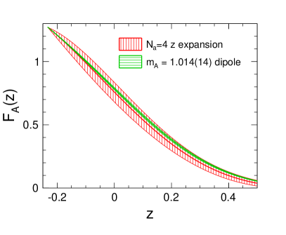
and as usual the error matrix is given by . This description can be systematically improved when and if further data or externally constrained deuterium models become available. The form factor is plotted versus and versus in Fig. 7, and compared with a previous world average dipole form factor from Ref. Bodek:2008epjc .

We also provide an alternate log-likelihood determination of the axial form factor to the range , but without deuteron systematic corrections. Central values and errors determined from are
| (73) |
The diagonal entries of the error matrix are
| (74) |
and the four-dimensional correlation matrix is
| (79) |
VII Applications
Having presented the axial form factor with errors and correlations amongst the coefficients, we may systematically compute derived observables that depend on this function. We consider several applications of our results.
VII.1 Axial radius
| Data set | |||
|---|---|---|---|
| () | () | () | |
| BNL 1981 | |||
| ANL 1982 | |||
| FNAL 1983 | |||
| Joint Fit |
We begin with the axial radius, defined in Eq. (27). While the radius by itself is not the only quantity of interest to neutrino scattering observables, it is only through the limit that a robust comparison can be made to other processes such as pion electroproduction.
The form factor coefficients and error matrix from the fit in Sec. VI determine the radius as
| (80) |
The constraint is much looser than would be obtained by restricting to the dipole model, cf. Table 4.141414Extractions of the radius from electroproduction data are also strongly influenced by the dipole assumption Bhattacharya:2011ah . For comparison, let us consider the constraints from individual experiments. Table 7 gives results for free parameters, with errors determined from the error matrix in Eqs. (67) and (72). The results from individual experiments are consistent with the joint fit. Note that the joint fit is not simply the average of the individual fits. This situation arises from a slight tension between data and Gaussian coefficient constraints (17) when comparing a single data set to the statistically more powerful combined data.
VII.2 Neutrino-nucleon quasielastic cross sections

Current and future neutrino oscillation experiments will precisely measure neutrino mixing parameters, determine the neutrino mass hierarchy, and search for possible CP violation and other new phenomena. This program relies on accurate predictions, with quantifiable uncertainties, for neutrino interaction cross sections. As the simplest examples, consider the charged-current quasielastic cross section for neutrino (antineutrino) scattering on an isolated neutron (proton).
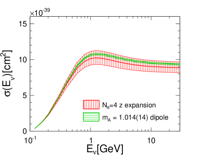
The best fit cross section and uncertainty are shown in Fig. 8, and compared to the prediction of dipole with axial mass Bodek:2008epjc . At representative energies, the cross sections and uncertainties shown in Fig. 8 are
| (81) |
for neutrinos and
| (82) |
for antineutrinos.
VII.3 Neutrino nucleus cross sections
Connecting nucleon-level information to experimentally observed neutrino-nucleus scattering cross sections requires data-driven modeling of nuclear effects. Our description of the axial form factor and uncertainty in Eqs. (66), (67), and (72) can be readily implemented in neutrino event generators that interface with nuclear models.151515The expansion will be available in GENIE production release v2.12.0. The code is currently available in the GENIE trunk prior to its official release. The module provides full generality of the expansion, and supports reweighting and error analysis with correlated parameters.
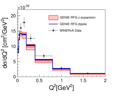
A multitude of studies and comparisons are possible. As illustration, consider MINERvA quasielastic data on carbon Fiorentini:2013ezn . Figure 9 shows a comparison of the distribution of measured events with the predictions from our , using a relativistic Fermi gas nuclear model in the default configuration of the GENIE v2.8 neutrino event generator Andreopoulos:2009rq . For comparison, we display the result obtained using a dipole with axial mass central value and error as quoted in the world average of Ref. Bodek:2008epjc . The central curves differ in their kinematic dependence, and the dipole result severely underestimates the uncertainty propagated from deuterium data.
The expansion implementation within GENIE includes a complete description of parameter errors and correlations. This will provide a systematic approach for testing different nuclear models and fitting nuclear model parameters, and for propagating uncertainties in nucleon-level amplitudes through to oscillation observables.
VII.4 Discussion
The dipole ansatz has been commonly used to parametrize the axial form factor in neutrino cross section predictions. The axial mass parameter in this ansatz often appears with either a very small uncertainty, e.g. Bodek:2008epjc , or a very large uncertainty, e.g. Abe:2015awa .
In the first case, the small error estimate results from the restrictive dipole ansatz, and is likely an underestimate of the actual uncertainty: as a point of comparison, the axial radius error is comparable to or smaller than the uncertainty on the proton charge radius Bernauer:2013tpr ; Lee:2015jqa . Recall that the charge radius is defined for the vector charge form factor analogously to the axial radius for the axial form factor. In contrast to the axial radius from neutrino-deuteron scattering, the charge radius from electron-proton scattering involves much higher statistics, a monoenergetic beam, and a simpler, proton, target.
In the second case, the large uncertainty on is typically included to account for tensions in external inputs from other experiments Abe:2015awa , and/or poorly constrained nuclear effects. Neither of these approaches is suited to the kinds of analyses that can be undertaken with modern cross section data such as the MINERvA example considered in Fig. 9. Underestimating nucleon-level uncertainties will bias conclusions about neutrino parameters or nuclear models. Inflating errors on within a dipole ansatz fails to capture the correct kinematic dependence of either nucleon-level uncertainties, or of nuclear corrections161616 Nondipole parametrizations have been considered in Amaro:2015lga ; Bodek:2007ym . Similar remarks apply to these examples. .
VIII Summary and conclusion
The constraints of elementary target data are critical to precision neutrino-nucleus cross sections underlying the accelerator neutrino program. Oscillation experiments rely on event rate predictions using nucleon-level amplitudes corrected for nuclear effects. Cross section experiments on nuclear targets can measure these nuclear effects but a complete accounting of uncertainty in nucleon-level amplitudes is critical for disentangling nucleon-level, nuclear-level, and flux uncertainties, and for determining final sensitivity to fundamental neutrino parameters.
The axial form factor is a prominent source of nucleon-level uncertainty. We have analyzed the world data set for quasielastic neutrino-deuteron scattering using a model-independent description of the axial form factor. Our final results are presented with central values (66), errors (67) and correlations (72). Any observable depending on the axial form factor may be computed from these results, with a complete error budget.
The axial radius, governing the shape of the axial form factor, is presented in Eq. (80). It has a significantly larger uncertainty than previously estimated based on the unjustified dipole ansatz. Benchmark total cross sections on nucleon targets are presented in Fig. 8 and Eqs. (VII.2) and (VII.2). The incorporation of nuclear effects with the RFG model is illustrated in Fig. 9.
The form factor and uncertainty budget presented here are important new inputs to the neutrino cross section effort. It is interesting to investigate potential impacts and interplay with a variety of other processes such as neutrinoless double beta decay matrix elements Simkovic:2007vu ; Holt:2013tda and the muon capture rate in muonic hydrogen Andreev:2012fj . The methodology presented can be revised or extended if new information becomes available. Future hydrogen or deuterium data would be trivial to include. Updated calculations for neutrino-deuteron scattering, especially if accompanied by an uncertainty, can be readily incorporated on top of this result. Lattice QCD holds promise to determine the axial form factor over much of the relevant range, in a manner that is free from nuclear corrections Bazavov:2009bb ; Dinter:2011plb ; Bazavov:2013prd ; Bhattacharya:2014prd ; Green:2014plb ; Bazavov:2015 .
Acknowledgments We thank L. Alvarez Ruso, J. R. Arrington, H. Budd, S. Bacca, A. Kronfeld, T. Mann, J. Morfin, G. Paz, and J. W. Van Orden for discussions, and R. Schiavilla for providing data files and interpretation of the results of Ref. Shen:2012xz . RG was supported by NSF Grant No. 1306944. Research of RJH and ASM was supported by DOE Grant No. DE-FG02-13ER41958. RG and RJH thank CETUP* (Center for Theoretical Underground Physics and Related Areas), for its hospitality and partial support during the 2014 Summer Program. Research of ASM also supported by the U.S. Department of Energy, Office of Science Graduate Student Research (SCGSR) program. The SCGSR program is administered by the Oak Ridge Institute for Science and Education for the DOE under contract number DE-AC05-06OR23100.
References
- (1) R. Acciarri et al. [DUNE Collaboration], arXiv:1512.06148 [hep-ex].
- (2) Y. Itow et al. [T2K Collaboration], hep-ex/0106019.
- (3) P. Adamson et al. [NOvA Collaboration], Phys. Rev. Lett. 116, no. 15, 151806 (2016) doi:10.1103/PhysRevLett.116.151806 [arXiv:1601.05022 [hep-ex]].
- (4) P. Adamson et al. [NOvA Collaboration], Phys. Rev. D 93, no. 5, 051104 (2016) doi:10.1103/PhysRevD.93.051104 [arXiv:1601.05037 [hep-ex]].
- (5) H. Chen et al. [MicroBooNE Collaboration], FERMILAB-PROPOSAL-0974.
- (6) C. Andreopoulos et al., Nucl. Instrum. Meth. A 614, 87 (2010) [arXiv:0905.2517 [hep-ph]].
- (7) Y. Hayato, Acta Phys. Polon. B 40, 2477 (2009).
- (8) O. Buss et al., Phys. Rept. 512, 1 (2012) doi:10.1016/j.physrep.2011.12.001 [arXiv:1106.1344 [hep-ph]].
- (9) T. Golan, C. Juszczak and J. T. Sobczyk, Phys. Rev. C 86, 015505 (2012) doi:10.1103/PhysRevC.86.015505 [arXiv:1202.4197 [nucl-th]].
- (10) D. Drakoulakos et al. [MINERvA Collaboration], hep-ex/0405002.
- (11) A. A. Aguilar-Arevalo et al. [MiniBooNE Collaboration], Phys. Rev. D 81, 092005 (2010) [arXiv:1002.2680 [hep-ex]].
- (12) A. A. Aguilar-Arevalo et al. [MiniBooNE Collaboration], Phys. Rev. D 83, 052007 (2011) [arXiv:1011.3572 [hep-ex]].
- (13) A. A. Aguilar-Arevalo et al. [MiniBooNE Collaboration], Phys. Rev. D 82, 092005 (2010) [arXiv:1007.4730 [hep-ex]].
- (14) K. Abe et al. [T2K Collaboration], Phys. Rev. D 91, no. 7, 072010 (2015) [arXiv:1502.01550 [hep-ex]].
- (15) C. Anderson et al. [ArgoNeuT Collaboration], Phys. Rev. Lett. 108, 161802 (2012) [arXiv:1111.0103 [hep-ex]].
- (16) P. A. Rodrigues et al. [MINERvA Collaboration], Phys. Rev. Lett. 116, 071802 (2016) doi:10.1103/PhysRevLett.116.071802 [arXiv:1511.05944 [hep-ex]].
- (17) G. D. Megias, J. E. Amaro, M. B. Barbaro, J. A. Caballero and T. W. Donnelly, arXiv:1603.08396 [nucl-th].
- (18) A. Lovato, S. Gandolfi, R. Butler, J. Carlson, E. Lusk, S. C. Pieper and R. Schiavilla, Phys. Rev. Lett. 111, no. 9, 092501 (2013) [arXiv:1305.6959 [nucl-th]].
- (19) S. Bacca and S. Pastore, J. Phys. G 41, no. 12, 123002 (2014) doi:10.1088/0954-3899/41/12/123002 [arXiv:1407.3490 [nucl-th]].
- (20) J. Carlson, S. Gandolfi, F. Pederiva, S. C. Pieper, R. Schiavilla, K. E. Schmidt and R. B. Wiringa, doi:10.1103/RevModPhys.87.1067 arXiv:1412.3081 [nucl-th].
- (21) G. Lee, J. R. Arrington and R. J. Hill, in preparation.
- (22) For a review see: K. A. Olive et al. [Particle Data Group Collaboration], Chin. Phys. C 38, 090001 (2014).
- (23) V. Lyubushkin et al. [NOMAD Collaboration], Eur. Phys. J. C 63, 355 (2009) [arXiv:0812.4543 [hep-ex]].
- (24) J. Brunner et al. [SKAT Collaboration], Z. Phys. C 45, 551 (1990).
- (25) M. Pohl et al. [GARGAMELLE NEUTRINO PROPANE Collaboration], Lett. Nuovo Cim. 26, 332 (1979).
- (26) L. B. Auerbach et al. [LSND Collaboration], Phys. Rev. C 66, 015501 (2002) [nucl-ex/0203011].
- (27) S. V. Belikov et al., Z. Phys. A 320, 625 (1985).
- (28) S. Bonetti, G. Carnesecchi, D. Cavalli, P. Negri, A. Pullia, M. Rollier, F. Romano and R. Schira, Nuovo Cim. A 38, 260 (1977).
- (29) For a review see: V. Bernard, L. Elouadrhiri and U. G. Meissner, J. Phys. G 28, R1 (2002) [hep-ph/0107088].
- (30) V. A. Andreev et al. [MuCap Collaboration], Phys. Rev. Lett. 110, no. 1, 012504 (2013) [arXiv:1210.6545 [nucl-ex]].
- (31) B. Bhattacharya, R. J. Hill and G. Paz, Phys. Rev. D 84, 073006 (2011) [arXiv:1108.0423 [hep-ph]].
- (32) R. J. Hill and G. Paz, Phys. Rev. D 82, 113005 (2010) doi:10.1103/PhysRevD.82.113005 [arXiv:1008.4619 [hep-ph]].
- (33) I. T. Lorenz and U. G. Meißner, Phys. Lett. B 737, 57 (2014) doi:10.1016/j.physletb.2014.08.010 [arXiv:1406.2962 [hep-ph]].
- (34) Z. Epstein, G. Paz and J. Roy, Phys. Rev. D 90, no. 7, 074027 (2014) doi:10.1103/PhysRevD.90.074027 [arXiv:1407.5683 [hep-ph]].
- (35) G. Lee, J. R. Arrington and R. J. Hill, Phys. Rev. D 92, 013013 (2015) [arXiv:1505.01489 [hep-ph]].
- (36) B. Bhattacharya, G. Paz and A. J. Tropiano, Phys. Rev. D 92, no. 11, 113011 (2015) doi:10.1103/PhysRevD.92.113011 [arXiv:1510.05652 [hep-ph]].
- (37) For a review and further references see: R. J. Hill, In the Proceedings of 4th Flavor Physics and CP Violation Conference (FPCP 2006), Vancouver, British Columbia, Canada, 9-12 Apr 2006, pp 027 [arXiv:hep-ph/0606023].
- (38) C. Bourrely, B. Machet and E. de Rafael, Nucl. Phys. B 189, 157 (1981).
- (39) C. G. Boyd, B. Grinstein and R. F. Lebed, Phys. Rev. Lett. 74, 4603 (1995) [arXiv:hep-ph/9412324].
- (40) C. G. Boyd, B. Grinstein and R. F. Lebed, Nucl. Phys. B 461, 493 (1996) [arXiv:hep-ph/9508211].
- (41) L. Lellouch, Nucl. Phys. B 479, 353 (1996) [arXiv:hep-ph/9509358].
- (42) I. Caprini, L. Lellouch and M. Neubert, Nucl. Phys. B 530, 153 (1998) [arXiv:hep-ph/9712417].
- (43) C. M. Arnesen, B. Grinstein, I. Z. Rothstein and I. W. Stewart, Phys. Rev. Lett. 95, 071802 (2005) [arXiv:hep-ph/0504209].
- (44) T. Becher and R. J. Hill, Phys. Lett. B 633, 61 (2006) [arXiv:hep-ph/0509090].
- (45) R. J. Hill, Phys. Rev. D 74, 096006 (2006) [arXiv:hep-ph/0607108].
- (46) C. Bourrely, L. Lellouch and I. Caprini, Phys. Rev. D 79, 013008 (2009) [arXiv:0807.2722 [hep-ph]].
- (47) A. Bharucha, T. Feldmann and M. Wick, JHEP 1009, 090 (2010) [arXiv:1004.3249 [hep-ph]].
- (48) Y. Amhis et al. [Heavy Flavor Averaging Group (HFAG) Collaboration], arXiv:1412.7515 [hep-ex].
- (49) C. Bouchard et al. [HPQCD Collaboration], Phys. Rev. D 88, no. 5, 054509 (2013) [Phys. Rev. D 88, no. 7, 079901 (2013)] doi:10.1103/PhysRevD.88.079901, 10.1103/PhysRevD.88.054509 [arXiv:1306.2384 [hep-lat]].
- (50) J. A. Bailey et al., Phys. Rev. D 93, no. 2, 025026 (2016) doi:10.1103/PhysRevD.93.025026 [arXiv:1509.06235 [hep-lat]].
- (51) R. R. Horgan, Z. Liu, S. Meinel and M. Wingate, Phys. Rev. D 89, no. 9, 094501 (2014) doi:10.1103/PhysRevD.89.094501 [arXiv:1310.3722 [hep-lat]].
- (52) J. A. Bailey et al. [Fermilab Lattice and MILC Collaborations], Phys. Rev. D 92, no. 1, 014024 (2015) doi:10.1103/PhysRevD.92.014024 [arXiv:1503.07839 [hep-lat]].
- (53) W. Detmold, C. Lehner and S. Meinel, Phys. Rev. D 92, no. 3, 034503 (2015) doi:10.1103/PhysRevD.92.034503 [arXiv:1503.01421 [hep-lat]].
- (54) K.S. Kuzmin, V. Lyubushkin, and V. Naumov, Eur. Phys. J. C 54, 517 (2008).
- (55) A. Bodek, S. Avvakumov, R. Bradford and H. S. Budd, Eur. Phys. J. C 53, 349 (2008)
- (56) G. A. Fiorentini et al. [MINERvA Collaboration], Phys. Rev. Lett. 111, 022502 (2013) doi:10.1103/PhysRevLett.111.022502 [arXiv:1305.2243 [hep-ex]].
- (57) W. A. Mann, U. Mehtani, B. Musgrave, Y. Oren, P. A. Schreiner, R. Singer, H. Yuta and R. Ammar et al., Phys. Rev. Lett. 31, 844 (1973).
- (58) S. J. Barish, J. Campbell, G. Charlton, Y. Cho, M. Derrick, R. Engelmann, L. G. Hyman and D. Jankowski et al., Phys. Rev. D 16, 3103 (1977).
- (59) K. L. Miller, S. J. Barish, A. Engler, R. W. Kraemer, B. J. Stacey, M. Derrick, E. Fernandez and L. Hyman et al., Phys. Rev. D 26, 537 (1982).
- (60) N. J. Baker, A. M. Cnops, P. L. Connolly, S. A. Kahn, H. G. Kirk, M. J. Murtagh, R. B. Palmer and N. P. Samios et al., Phys. Rev. D 23, 2499 (1981).
- (61) T. Kitagaki, S. Tanaka, H. Yuta, K. Abe, K. Hasegawa, A. Yamaguchi, K. Tamai and T. Hayashino et al., Phys. Rev. D 28, 436 (1983).
- (62) T. Kitagaki et al., Phys. Rev. D 42, 1331 (1990). doi:10.1103/PhysRevD.42.1331
- (63) M. G. Olsson, E. T. Osypowski and E. H. Monsay, Phys. Rev. D 17, 2938 (1978). See in particular Eq.(5).
- (64) R. Bradford, A. Bodek, H. S. Budd and J. Arrington, Nucl. Phys. Proc. Suppl. 159, 127 (2006) [hep-ex/0602017].
- (65) S. K. Singh, Nucl. Phys. B 36, 419 (1972).
- (66) H. S. Budd, A. Bodek and J. Arrington, hep-ex/0308005.
- (67) A. Bodek, S. Avvakumov, R. Bradford and H. S. Budd, Eur. Phys. J. C 53, 349 (2008) doi:10.1140/epjc/s10052-007-0491-4 [arXiv:0708.1946 [hep-ex]].
- (68) R. Pohl et al., Nature 466, 213 (2010).
- (69) J. C. Bernauer et al. [A1 Collaboration], Phys. Rev. C 90, no. 1, 015206 (2014) [arXiv:1307.6227 [nucl-ex]].
- (70) G. Shen, L. E. Marcucci, J. Carlson, S. Gandolfi and R. Schiavilla, Phys. Rev. C 86, 035503 (2012) [arXiv:1205.4337 [nucl-th]].
- (71) C. H. Llewellyn Smith, Phys. Rept. 3, 261 (1972).
- (72) See supplemental material included with the e-Print [arXiv:1603.03048 [hep-ph]] for the digitized and files from the ANL, BNL, and FNAL experiments as well as smeared distributions.
- (73) S. J. Barish et al., Phys. Rev. D 19, 2521 (1979). doi:10.1103/PhysRevD.19.2521
- (74) A. Bodek, H. S. Budd and J. Arrington, AIP Conf. Proc. 698, 148 (2004) doi:10.1063/1.1664214 [hep-ex/0309024].
- (75) H. S. Budd, A. Bodek and J. Arrington, Nucl. Phys. Proc. Suppl. 139, 90 (2005) doi:10.1016/j.nuclphysbps.2004.11.181 [hep-ex/0410055].
- (76) G. P. Lepage and S. J. Brodsky, Phys. Rev. D 22, 2157 (1980).
- (77) K. L. Miller, Ph.D. Thesis, Carnegie Mellon University (1981) UMI-92-09392.
- (78) M. Martini, M. Ericson, G. Chanfray, and J. Marteau, Phys. Rev. C 80, 065501 (2009).
- (79) R. Gran, J. Nieves, F. Sanchez, and M. J. Vicente Vacas, Phys. Rev. D 88, 113007 (2013).
- (80) S. K. Singh and H. Arenhovel, Z. Phys. A 324, 347 (1986).
- (81) O. Moreno, T. W. Donnelly, J. W. Van Orden and W. P. Ford, Phys. Rev. D 92, no. 5, 053006 (2015) doi:10.1103/PhysRevD.92.053006 [arXiv:1508.00492 [hep-ph]].
- (82) M. Betancourt, Muon Neutrino CCQE at MINERvA, in preparation, Nuint 2015 conference proceedings.
- (83) J. E. Amaro and E. Ruiz Arriola, Phys. Rev. D 93, no. 5, 053002 (2016) doi:10.1103/PhysRevD.93.053002 [arXiv:1510.07532 [nucl-th]].
- (84) F. Simkovic, A. Faessler, V. Rodin, P. Vogel and J. Engel, Phys. Rev. C 77, 045503 (2008) doi:10.1103/PhysRevC.77.045503 [arXiv:0710.2055 [nucl-th]].
- (85) J. D. Holt and J. Engel, Phys. Rev. C 87, no. 6, 064315 (2013) doi:10.1103/PhysRevC.87.064315 [arXiv:1304.4202 [nucl-th]].
- (86) For a review and further references, see: A. Bazavov et al. [MILC Collaboration], Rev. Mod. Phys. 82, 1349 (2010) doi:10.1103/RevModPhys.82.1349 [arXiv:0903.3598 [hep-lat]].
- (87) S. Dinter et al., Phys. Lett. B 704, 89 (2011)
- (88) A. Bazavov et al., Phys. Rev. D 87, 054505 (2013).
- (89) T. Bhattacharya et al., Phys. Rev. D 89, 094502 (2014) [arXiv:1306.5435 [hep-lat]].
- (90) J.R. Green et al., Phys. Lett. B 734, 290 (2014)
- (91) A. Bazavov, et al. (Fermilab Lattice and MILC Collaborations), “The Nucleon Axial-Vector Form Factor at the Physical Point with HISQ Ensembles,” (2015), proposal to USQCD.