Geometric estimation of a potential and cone conditions of a body

Abstract

We investigate a potential obtained as the convolution of a radially symmetric function and the characteristic function of a body (the closure of a bonded open set) with exterior cones. In order to restrict the location of a maximizer of the potential into a smaller closed region contained in the interior of the body, we give an estimate of the potential using the exterior cones of the body. Moreover, we apply the result to the Poisson integral for the upper half space.

Keywords and phrases. Hot spot, Poisson integral, solid angle, illuminating center, Riesz potential, Hadamard finite part, renormalization, $r^{\alpha-m}$-potential, minimal unfolded region, heart, cone condition.
2010 Mathematics Subject Classification: 31B25, 35B38, 35B50, 51M16, 52A40.

1 Introduction

Let $\Omega$ be a body (the closure of a bounded open set) in $\mathbb{R}^{m}$. We consider a potential of the form

$$K_{\Omega}(x,t)=\int_{\Omega}k\left(\left|x-\xi\right|,t\right)d\xi,\ x\in\mathbb{R}^{m},\ t>0,$$ (1.1)

and investigate its spatial maximizer.

When $k(r,t)$ is given by the Gauss kernel, the potential $K_{\Omega}(x,t)$ is the solution of the Cauchy problem for the heat equation with initial datum $\chi_{\Omega}$,

$$W_{\Omega}(x,t)=\frac{1}{\left(4\pi t\right)^{m/2}}\int_{\Omega}\exp\left(-\frac{\left|x-\xi\right|^{2}}{4t}\right)d\xi,\ x\in\mathbb{R}^{m},\ t>0.$$ (1.2)

A spatial maximizer of $W_{\Omega}$ is called a hot spot of $\Omega$ at time $t$.

In [4], Chavel and Karp showed that $\Omega$ has a hot spot for each $t$, that any hot spot belongs to the convex hull of $\Omega$, and that the set of hot spots converges to the one-point set of the centroid (center of mass) of $\Omega$ as $t$ goes to infinity with respect to the Hausdorff distance. Furthermore, calculating the Hessian of $W_{\Omega}(\cdot,t):\mathbb{R}^{m}\to\mathbb{R}$, in [9], Jimbo and Sakaguchi indicated that $\Omega$ has a unique hot spot whenever $t\geq(\operatorname{diam}\Omega)^{2}/2$. Roughly speaking, the large-time behavior of hot spots was studied in [4, 9]. (To tell the truth, in [4, 9], the above properties of hot spots were shown for a non-zero non-negative bounded compactly supported initial datum. But, in this paper, we are interested in the case where the initial datum is given by the characteristic function of a body.)

In contrast, in [10], Karp and Peyerimhoff gave a geometric heat comparison criteria and investigated the small-time behavior of hot spots. Roughly speaking, they compared two heat flows for two points in two different bodies by using the distance functions from the complements and showed that any sequence of hot spots of $\Omega$ at time $t_{\ell}$ converges to an incenter of $\Omega$ as $t_{\ell}$ tends to zero. Let us review their exact statement as below: Let $X$ and $Y$ be bodies in $\mathbb{R}^{m}$; Fix two constants $R>S\geq 0$; Let $X^{\prime}=\{x\in X|\operatorname{dist}(x,X^{c})\geq R\}$, and $Y^{\prime}=\{y\in\mathbb{R}^{m}|\operatorname{dist}(y,Y^{c})\leq S\}$; Then, we can choose a small time $\tau$ such that if $0<t<\tau$, then, for any $x\in X^{\prime}$ and $y\in Y^{\prime}$, we have $H_{X}(x,t)>H_{Y}(y,t)$; Taking $X=Y=\Omega$ and $R=R_{\infty}(\Omega)=\max\operatorname{dist}(\xi,\Omega^{c})$ (the inradius), we can conclude that, for any decreasing sequence $\{t_{\ell}\}$ with zero limiting value and any hot spot $h(t_{\ell})$ of $\Omega$ at time $t_{\ell}$, the distance between $h(t_{\ell})$ and the set of incenters $\mathcal{I}_{\Omega}=\{\xi\in\Omega|\operatorname{dist}(\xi,\Omega^{c})=R_{\infty}(\Omega)\}$ tends to zero as $\ell$ goes to infinity. (To tell the truth, they investigated the above comparison theorem in Riemannian manifolds. But, in this paper, we are interested in Euclidean case.) We also refer to [12, pp. 2–3] for the small-time behavior of hot spots.

On the other hand, in [19], for the kernel $k$ in (1.1), the author gave a sufficient condition implying the results shown in [4, 9]. As a by-product, for example, his sufficient condition can be applied to the Poisson integral for the upper half space,

$$P_{\Omega}(x,h)=\frac{2h}{\sigma_{m}\left(S^{m}\right)}\int_{\Omega}\left(\left|x-\xi\right|^{2}+h^{2}\right)^{-(m+1)/2}d\xi,\ x\in\mathbb{R}^{m},\ h>0,$$ (1.3)

where $\sigma_{m}$ denotes the $m$-dimensional spherical Lebesgue measure. Precisely, his sufficient condition implies that the function $P_{\Omega}(\cdot,h):\mathbb{R}^{m}\to\mathbb{R}$ has a maximizer for each $h$, that any maximizer of $P_{\Omega}(\cdot,h)$ belongs to the convex hull of $\Omega$, that the set of maximizers of $P_{\Omega}(\cdot,h)$ converges to the one-point set of the centroid of $\Omega$ as $h$ goes to infinity with respect to the Hausdorff distance, and that $P_{\Omega}(\cdot,h)$ has a unique maximizer whenever $h\geq\sqrt{m+2}\operatorname{diam}\Omega$.

Here, we remark that the Poisson integral $P_{\Omega}$ satisfies the Laplace equation for the upper half space, that is,

$$\left(\sum_{j=1}^{m}\frac{\partial^{2}}{\partial x_{j}^{2}}+\frac{\partial^{2}}{\partial h^{2}}\right)P_{\Omega}(x,h)=0,\ x\in\mathbb{R}^{m},\ h>0,$$ (1.4)

and we have the boundary condition

$$\lim_{h\to 0^{+}}P_{\Omega}(x,h)=\chi_{\Omega}(x),\ x\in\mathbb{R}^{m}\setminus\partial\Omega.$$ (1.5)

In order to understand the geometric meaning of the author’s results on maximizers of $P_{\Omega}(\cdot,h)$, let $A_{\Omega}=\sigma_{m}(S^{m})P_{\Omega}/2$. The function $A_{\Omega}$ is obtained in the following manner: Let $x$ be a point in $\mathbb{R}^{m}$, and $h$ a positive constant; Define the map

$$p_{(x,h)}:\Omega\times\{0\}\ni(\xi,0)\mapsto\frac{(\xi,0)-(x,h)}{\left|(\xi,0)-(x,h)\right|}\in S^{m};$$ (1.6)

The solid angle of $\Omega$ at $(x,h)$ is defined as the $m$-dimensional spherical Lebesgue measure of the image $p_{(x,h)}(\Omega)$ (see Figure 1), and direct calculation shows

$$\sigma_{m}\left(p_{(x,h)}(\Omega)\right)=h\int_{\Omega}\left(\left|x-\xi\right|^{2}+h^{2}\right)^{-(m+1)/2}d\xi=A_{\Omega}(x,h).$$ (1.7)

In [22], the solid angle of $\Omega$ as $(x,h)$ was regarded as the “brightness” of $\Omega$ having a light source at $(x,h)$. We call a maximizer of $A_{\Omega}(\cdot,h)$ an illuminating center of $\Omega$ of height $h$. Thus, the properties of $P_{\Omega}$ shown in [19] are understood as the large-height behavior of illuminating centers. In other words, it was shown that the large-parameter behavior of spatial maximizers of $P_{\Omega}$ is similar to that of $W_{\Omega}$.

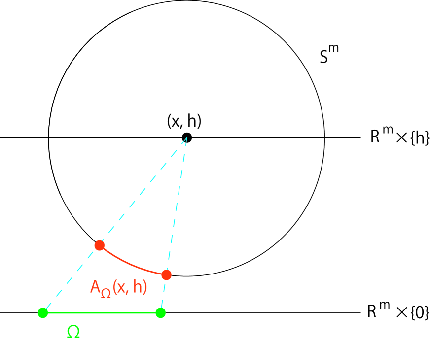
Figure 1: The solid angle of $\Omega$ at $(x,h)$

From such backgrounds, in this paper, in order to compare small-parameter behavior of spatial maximizers of $P_{\Omega}$ and $W_{\Omega}$, we mainly investigate the small-height behavior of illuminating centers. Informal computation shows

$$\frac{A_{\Omega}(x,h)}{h}=\int_{\Omega}\left(\left|x-\xi\right|^{2}+h^{2}\right)^{-(m+1)/2}d\xi\to\int_{\Omega}\left|x-\xi\right|^{-(m+1)}d\xi$$ (1.8)

as $h$ tends to $0^{+}$. But the right hand side diverges whenever $x$ is in $\Omega$. Then, for a point $x$ in the interior of $\Omega$, let us consider its Hadamard finite part,

$$V_{\Omega}^{(-1)}(x) =\lim_{\varepsilon\to 0^{+}}\left(\int_{\Omega\setminus B_{\varepsilon}(x)}\left|x-\xi\right|^{-(m+1)}-\frac{\sigma_{m-1}\left(S^{m-1}\right)}{\varepsilon}\right)$$ (1.9)

$$=\int_{\Omega\setminus B_{\varepsilon}(x)}\left|x-\xi\right|^{-(m+1)}-\frac{\sigma_{m-1}\left(S^{m-1}\right)}{\varepsilon}.$$ (1.10)

Here, we remark that the latter equality (1.10) holds whenever $0<\varepsilon<\operatorname{dist}(x,\Omega^{c})$ (see Proposition 2.7).

It is expected that any sequence of illuminating centers of height $h_{\ell}$ converges to a maximizer of $V_{\Omega}^{(-1)}$ as $h_{\ell}$ tends to zero. This expectation comes from the following procedure: Let $\varepsilon>0$ be small enough; Suppose that, for any small enough $h>0$, any illuminating center is at least $\varepsilon$ away from the boundary of $\Omega$; Since the Poisson kernel is radially symmetric, the solid angle of $B_{\varepsilon}(x)$ at $(x,h)$ depends only on $\varepsilon$ and $h$; Decomposing the solid angle function as $A_{\Omega}(x,h)=A_{\Omega\setminus B_{\varepsilon}(x)}(x,h)+A_{B_{\varepsilon}(x)}(x,h)$, a point $c(h)$ is an illuminating center if and only if it is a maximizer of $A_{\Omega\setminus B_{\varepsilon}(\cdot)}(\cdot,h)$; As $h$ tends to zero, the kernel $(|x-\xi|^{2}+h^{2})^{-(m+1)/2}$ converges to $|x-\xi|^{-(m+1)}$ uniformly for $\xi$ in $\Omega\setminus B_{\varepsilon}(x)$; Roughly speaking, if the height parameter $h$ is small enough, then we have

$$\frac{A_{\Omega}(x,h)}{h}=\frac{A_{\Omega\setminus B_{\varepsilon}(x)}(x,h)}{h}+\frac{A_{B_{\varepsilon}(x)}(x,h)}{h}\approx V_{\Omega}^{(-1)}(x)+\frac{\sigma_{m-1}\left(S^{m-1}\right)}{\varepsilon}+\frac{A_{B_{\varepsilon}(x)}(x,h)}{h}$$ (1.11)

for any point $x$ in the interior of $\Omega$ with $\operatorname{dist}(x,\Omega^{c})>\varepsilon$.

In order to formulate the above procedure, we have to give a closed subset in the interior of $\Omega$ such that it contains all the illuminating centers for any small enough $h>0$. This is because we can use the expression (1.10) of the potential $V_{\Omega}^{(-1)}$ only in the interior of $\Omega$. Namely, in (1.10), we want to take a uniform $\varepsilon$ for illuminating centers of any small enough height and maximizers of $V_{\Omega}^{(-1)}$.

We refer to [1, 2, 17, 18, 19, 20] for the study on the location of maximizers of a potential. Some authors tried to restrict the location of maximizers of a potential into a smaller region. Using the moving plane argument ([5, 21]), all the maximizers of a potential with a radially symmetric strictly decreasing kernel are contained in the minimal unfolded region of $\Omega$. (The minimal unfolded region is sometimes called the heart.) But, in general, the minimal unfolded region of $\Omega$ is not contained in the interior of $\Omega$ (see Example 2.22).

In this paper, assuming the uniform interior cone condition for the complement of the body $\Omega$ (see Definition 2.1) and taking the following three steps, we formulate the above procedure:

Step 1.

We give a constant $0<\tilde{R}<R_{\infty}(\Omega)$ such that, for any $x\in\Omega$ with $\operatorname{dist}(x,\Omega^{c})=R_{\infty}(\Omega)$ and $y\in\Omega$ with $\operatorname{dist}(y,\Omega^{c})\leq\tilde{R}$, we have $V_{\Omega}^{(-1)}(y)<V_{\Omega}^{(-1)}(x)$. Namely, any maximizer of $V_{\Omega}^{(-1)}$ belongs to the inner-parallel body of $\Omega$ of radius $\tilde{R}$.

Step 2.

For any constant $0<b<1$, there exits a positive $h_{0}$ such that if $0<h<h_{0}$, then, for any $x\in\Omega$ with $\operatorname{dist}(x,\Omega^{c})=R_{\infty}(\Omega)$ and $y\in\mathbb{R}^{m}$ with $\operatorname{dist}(y,\Omega^{c})\leq b\tilde{R}$, we have $A_{\Omega}(y,h)<A_{\Omega}(x,h)$. Namely, if $h$ is sufficiently small, then any illuminating center belongs to the inner-parallel body of $\Omega$ of radius $b\tilde{R}$.

Step 3.

The limit point of any illuminating center of height $h_{\ell}$ must be a maximizer of $V_{\Omega}^{(-1)}$.

Moreover, the above argument can be extended to a general case. Precisely, we give the same estimate as in the first step to the Hadamard finite part of the Riesz potential,

$$V_{\Omega}^{(\alpha)}(x)=\begin{cases}\displaystyle\lim_{\varepsilon\to 0^{+}}\left(\int_{\Omega\setminus B_{\varepsilon}(x)}\left|x-\xi\right|^{\alpha-m}d\xi-\frac{\sigma_{m-1}\left(S^{m-1}\right)}{-\alpha}\varepsilon^{\alpha}\right)&(\alpha<0),\\ \displaystyle\lim_{\varepsilon\to 0^{+}}\left(\int_{\Omega\setminus B_{\varepsilon}(x)}\left|x-\xi\right|^{-m}d\xi-\sigma_{m-1}\left(S^{m-1}\right)\log\frac{1}{\varepsilon}\right)&(\alpha=0).\end{cases}$$ (1.12)

Also, we give the same estimate as in the second step to a potential of the form (1.1). In other words, our main result in this paper is the estimate of a potential like the second step, and, as its by-product, we derive the small-height behavior of illuminating centers.

Throughout this paper, $\overset{\mbox{\tiny$\circ$}}{X}$, $\bar{X}$, $X^{c}$, $R_{\infty}(X)$ and $\operatorname{diam}X$ denote the interior, the closure, the complement, the inradius and the diameter of a set $X$ in $\mathbb{R}^{m}$, respectively. For a set $X$ in $\mathbb{R}^{m}$ and a positive constant $\rho$, the symbol $X\sim\rho B^{m}$ denotes the inner-parallel body of $X$ of radius $\rho$, that is, $X\sim\rho B^{m}=\{x\in X|\operatorname{dist}(x,X^{c})\geq\rho\}$. We denote the $m$-dimensional closed ball of radius $\rho$ and centered at $x$ by $B_{\rho}(x)=\rho B^{m}+x$. We denote a point $x$ in $\mathbb{R}^{m}$ by $x=\left(x_{1},\ldots,x_{m}\right)$. The $N$-dimensional spherical Lebesgue measure is denoted by $\sigma_{N}$. In particular, the symbol $\sigma$ is used in the case of $N=m-1$, for short.

Acknowledgements. The author would like to express his deep gratitude to Professor Jun O’Hara, Professor Kazushi Yoshitomi and Professor Hiroaki Aikawa. O’Hara gave him kind advice throughout writing this paper. Yoshitomi informed him of some cone conditions. Aikawa informed him of the proof of Lemma 2.3 and Remark 2.5.

2 Preliminaries

2.1 Cone conditions

Let us prepare the cone conditions which are related to the complexity of the boundary of a body. Throughout this paper, we understand that $C$ is an open cone of vertex $x$, axis direction $v$, aperture angle $\kappa$ and height $\delta$ if $C$ is given as

$$C=\left\{x+\rho Rv\left|0<\rho<\delta,\ R\in SO(m),\ Rv\cdot v>\cos\frac{\kappa}{2}\right\}\right..$$ (2.1)

Definition 2.1.

An open set $U$ in $\mathbb{R}^{m}$ satisfies the uniform interior cone condition if there exists an open cone $C$ in $\mathbb{R}^{m}$ such that, for each point $x\in U$, we can take an open cone of vertex $x$ contained in $U$ and congruent to $C$.

Definition 2.2.

An open set $U$ in $\mathbb{R}^{m}$ satisfies the uniform boundary inner cone condition if there exists an open cone $C$ in $\mathbb{R}^{m}$ such that, for each point $x\in\partial U$, we can take an open cone of vertex $x$ contained in $U$ and congruent to $C$.

The proof of the following Lemma is due to Hiroaki Aikawa.

Lemma 2.3.

Let $U$ be an open set in $\mathbb{R}^{m}$. If $U$ satisfies the uniform interior cone condition for an open cone $C$ of aperture angle $\kappa$ and height $\delta$, then it also satisfies the uniform boundary inner cone condition for the cone $C$.

Proof.

Fix a point $x$ on the boundary of $U$. For each natural number $n$, we take a point $\xi^{n}$ from $B_{1/n}(x)\cap U$. Thanks to the uniform interior cone condition of $U$, we can take an open cone $C(\xi^{n})$ of vertex $\xi^{n}$ contained in $U$ and congruent to $C$. Let $v^{n}$ be the axis direction of $C(\xi^{n})$. Since the unit sphere $S^{m-1}$ is compact in $\mathbb{R}^{m}$, we may assume that the sequence $\{v^{n}\}$ converges to a direction $v$.

Let $C(x)$ be the open cone of vertex $x$ and axis direction $v$ congruent to $C$. We show that $C(x)$ is contained in $U$. Suppose that $C(x)$ is not contained in $U$. We take a point from $C(x)\cap U^{c}$. The point can be expressed as $x+\rho Rv$ for some $0<\rho<\delta$ and rotation matrix $R$ with $Rv\cdot v>\cos(\kappa/2)$. We remark that the point $\xi^{n}+\rho Rv^{n}$ is in $C(\xi^{n})$. Since $C(\xi^{n})$ is contained in $U$ for any $n$, we have

$$\left|\left(x+\rho Rv\right)-\left(\xi^{n}+\rho Rv^{n}\right)\right|\geq\operatorname{dist}\left(\xi^{n}+\rho Rv^{n},U^{c}\right)\geq\min\left\{\delta-\rho,\ \rho\sin\left(\frac{\kappa}{2}-\theta\right)\right\},$$

where $\theta=\arccos(Rv\cdot v)$. On the other hand, for any large enough $n$,

$$\left|\left(x+\rho Rv\right)-\left(\xi^{n}+\rho Rv^{n}\right)\right|<\frac{1}{2}\min\left\{\delta-\rho,\ \rho\sin\left(\frac{\kappa}{2}-\theta\right)\right\},$$

which is a contradiction. ∎

Remark 2.4.

Let $\Omega$ be a body (the closure of a bounded open set) in $\mathbb{R}^{m}$. Regarding a half space as a cone of aperture angle $\pi$ and height $+\infty$, $\Omega$ is convex if and only if the complement of $\Omega$ satisfies the uniform boundary inner cone condition of aperture angle $\pi$ and height $+\infty$.

Remark 2.5.

In Lemma 2.3, for an open set $U$, we showed that the uniform interior cone condition implies the uniform boundary inner cone condition. We remark that the converse statement does not always hold. For example, let us consider an open unit disc and remove a cusp from the disc near the center. Let $U$ be such an open set. Then, $U$ satisfies the uniform boundary inner cone condition but not the uniform interior cone condition.

The author would like to express his gratitude to Professor Hiroaki Aikawa for informing him of this example.

Problem 2.6.

Let $U$ be the interior of a body in $\mathbb{R}^{m}$. Does the uniform boundary inner cone condition of $U$ imply the uniform interior cone condition of $U$?

2.2 Renormalization of the Riesz potential

Let $\Omega$ be a body (the closure of a bounded open set) in $\mathbb{R}^{m}$. We consider the Riesz potential of $\Omega$ of order $0<\alpha<m$,

$$V_{\Omega}^{(\alpha)}(x)=\int_{\Omega}\left|x-\xi\right|^{\alpha-m}d\xi,\ x\in\mathbb{R}^{m}.$$ (2.2)

We remark that if $\alpha\leq 0$, then the above integral diverges for any interior point $x$ of $\Omega$. In [17], O’Hara extended the potential $V_{\Omega}^{(\alpha)}$ to the case of $\alpha\leq 0$ by using the same renormalizing process as in the definition of his energy of knots introduced in [15, 16]. Precisely, for $\alpha\leq 0$ and $x\in\overset{\mbox{\tiny$\circ$}}{\Omega}$, define the renormalization of the Riesz potential

$$V_{\Omega}^{(\alpha)}(x)=\begin{cases}\displaystyle\lim_{\varepsilon\to 0^{+}}\left(\int_{\Omega\setminus B_{\varepsilon}(x)}\left|x-\xi\right|^{\alpha-m}d\xi-\frac{\sigma\left(S^{m-1}\right)}{-\alpha}\varepsilon^{\alpha}\right)&(\alpha<0),\\ \displaystyle\lim_{\varepsilon\to 0^{+}}\left(\int_{\Omega\setminus B_{\varepsilon}(x)}\left|x-\xi\right|^{-m}d\xi-\sigma\left(S^{m-1}\right)\log\frac{1}{\varepsilon}\right)&(\alpha=0),\end{cases}$$ (2.3)

and we call it the $r^{\alpha-m}$-potential of order $\alpha$ in what follows. Here, for $\alpha\leq 0$ and $x\in\Omega^{c}$, we define the potential $V_{\Omega}^{(\alpha)}(x)$ as the usual Riesz potential, that is,

$$V_{\Omega}^{(\alpha)}(x)=\int_{\Omega}\left|x-\xi\right|^{\alpha-m}d\xi,\ \alpha\leq 0,\ x\in\Omega^{c}.$$ (2.4)

Let us prepare some terminologies and properties of $V_{\Omega}^{(\alpha)}$ from [17].

Proposition 2.7 ([17, Proposition 2.5]).

Let $\Omega$ be a body in $\mathbb{R}^{m}$. For $\alpha\leq 0$ and $x\in\overset{\mbox{\tiny$\circ$}}{\Omega}$, we have

$$V_{\Omega}^{(\alpha)}(x)=\begin{cases}\displaystyle\int_{\Omega\setminus B_{\varepsilon}(x)}\left|x-\xi\right|^{\alpha-m}d\xi-\frac{\sigma\left(S^{m-1}\right)}{-\alpha}\varepsilon^{\alpha}&(\alpha<0),\\ \displaystyle\int_{\Omega\setminus B_{\varepsilon}(x)}\left|x-\xi\right|^{-m}d\xi-\sigma\left(S^{m-1}\right)\log\frac{1}{\varepsilon}&(\alpha=0)\end{cases}$$

whenever $\varepsilon<\operatorname{dist}(x,\Omega^{c})$. In particular, for $\alpha<0$ and $x\in\overset{\mbox{\tiny$\circ$}}{\Omega}$, we have

$$V_{\Omega}^{(\alpha)}(x)=-\int_{\Omega^{c}}\left|x-\xi\right|^{\alpha-m}d\xi.$$

Since this statement will play an important role in this paper, we review its proof (see also [17, Lemma 2.4]).

Proof.

We show the statement in the case of $\alpha<0$. Replacing the renormalization term, the proof in the case of $\alpha=0$ goes parallel.

Fix an arbitrary interior point $x$ of $\Omega$. Let $0<\delta<\varepsilon<\operatorname{dist}(x,\Omega^{c})$. Since we have

$$\Omega\setminus B_{\varepsilon}(x)=(\Omega\setminus B_{\delta}(x))\setminus(B_{\varepsilon}(x)\setminus B_{\delta}(x)),$$

we get

$$\int_{\Omega\setminus B_{\varepsilon}(x)}\left|x-\xi\right|^{\alpha-m}d\xi =\left(\int_{\Omega\setminus B_{\delta}(x)}\left|x-\xi\right|^{\alpha-m}d\xi-\frac{\sigma\left(S^{m-1}\right)}{-\alpha}\delta^{\alpha}\right)$$

$$\quad-\left(\int_{B_{\varepsilon}(x)\setminus B_{\delta}(x)}\left|x-\xi\right|^{\alpha-m}d\xi-\frac{\sigma\left(S^{m-1}\right)}{-\alpha}\delta^{\alpha}\right).$$

Since the left hand side is independent of $\delta$, taking the limit $\delta\to 0^{+}$, we obtain

$$\int_{\Omega\setminus B_{\varepsilon}(x)}\left|x-\xi\right|^{\alpha-m}d\xi=V_{\Omega}^{(\alpha)}(x)+\frac{\sigma\left(S^{m-1}\right)}{-\alpha}\varepsilon^{\alpha},$$

which completes the proof. ∎

Proposition 2.7 and the definition (2.4) guarantee the continuity of $V_{\Omega}^{(\alpha)}$.

Proposition 2.8 ([17, Proposition 2.12]).

Let $\Omega$ be a body in $\mathbb{R}^{m}$. For $\alpha\leq 0$, the restrictions of $V_{\Omega}^{(\alpha)}$ to the interior and the complement of $\Omega$ are continuous.

Assuming the uniform boundary inner cone condition and using Proposition 2.7, we can understand the behavior of the potential $V_{\Omega}^{(\alpha)}$ near the boundary of $\Omega$.

Lemma 2.9 ([17, Lemma 2.13]).

Let $\Omega$ be a body in $\mathbb{R}^{m}$, and $\alpha\leq 0$.

1. If the complement of $\Omega$ satisfies the uniform boundary inner cone condition, then the potential $V_{\Omega}^{(\alpha)}(x)$ diverges to $-\infty$ uniformly as $x\in\overset{\mbox{\tiny$\circ$}}{\Omega}$ approaches to any boundary point of $\Omega$.

2. If the interior of $\Omega$ satisfies the uniform boundary inner cone condition, then the potential $V_{\Omega}^{(\alpha)}(x)$ diverges to $+\infty$ uniformly as $x\in\Omega^{c}$ approaches to any boundary point of $\Omega$.

This Lemma will play an important role in section 3. Let us review its proof.

Proof.

We show the first assertion. The proof of the second assertion goes parallel.

Suppose that the complement of $\Omega$ satisfies the uniform boundary inner cone condition for an open cone $C$ of vertex $0$, aperture angle $\kappa$ and height $\delta$. Fix an arbitrary point $z$ on the boundary of $\Omega$. We can take an open cone $C(z)$ of vertex $z$ contained in the complement of $\Omega$ and congruent to $C$.

We first show the statement in the case of $\alpha<0$. Let $\varepsilon$ be a positive constant, and take a point $x\in\overset{\mbox{\tiny$\circ$}}{\Omega}\cap B_{\varepsilon}(z)$. By Proposition 2.7, we can estimate the potential $V_{\Omega}^{(\alpha)}$ as

$$-V_{\Omega}^{(\alpha)}(x)\geq\int_{C(z)}\left|x-\xi\right|^{\alpha-m}d\xi\geq\frac{\sigma\left(C\cap\delta S^{m-1}\right)}{\delta^{m-1}}\int_{0}^{\delta}\left(\rho+\varepsilon\right)^{\alpha-m}\rho^{m-1}d\rho$$

which diverges to $+\infty$ as $\varepsilon$ tends to zero.

Next, we consider the case of $\alpha=0$. By proposition 2.7, for any interior point $x$ of $\Omega$ and positive constant $\varepsilon<\operatorname{dist}(x,\Omega^{c})$, we have

$$\int_{\Omega\setminus B_{\varepsilon}(x)}\left|x-\xi\right|^{-m}d\xi-\sigma\left(S^{m-1}\right)\log\frac{1}{\varepsilon}$$

$$=\int_{\Omega\setminus B_{\varepsilon}(x)}\left|x-\xi\right|^{-m}d\xi-\int_{B_{\operatorname{diam}\Omega}(x)\setminus B_{\varepsilon}(x)}\left|x-\xi\right|^{-m}d\xi+\sigma\left(S^{m-1}\right)\log\operatorname{diam}\Omega$$

$$=\sigma\left(S^{m-1}\right)\log\operatorname{diam}\Omega-\int_{B_{\operatorname{diam}\Omega}(x)\setminus\Omega}\left|x-\xi\right|^{-m}d\xi.$$

Thus, in the same argument as in the case of $\alpha<0$, we obtain the conclusion. ∎

Thanks to Proposition 2.8 and Lemma 2.9, for $\alpha\leq 0$, the restriction of $V_{\Omega}^{(\alpha)}$ to the interior of $\Omega$ has a maximizer.

Theorem 2.10 ([17, Theorem 3.5]).

Let $\Omega$ be a body in $\mathbb{R}^{m}$. Suppose that the complement of $\Omega$ satisfies the uniform boundary inner cone condition. For $\alpha\leq 0$, the restriction of $V_{\Omega}^{(\alpha)}$ to the interior of $\Omega$ has a maximizer.

Definition 2.11 ([17, Definition 3.1]).

Let $\Omega$ be a body in $\mathbb{R}^{m}$. An interior point $c$ of $\Omega$ is called an $r^{\alpha-m}$-center of $\Omega$ if it gives the maximum value of the restriction of $V_{\Omega}^{(\alpha)}$ to the interior of $\Omega$. Let us denote the set of $r^{\alpha-m}$-centers by $\mathcal{V}_{\Omega}(\alpha)$, that is,

$$\mathcal{V}_{\Omega}(\alpha)=\left\{c\in\overset{\mbox{\tiny$\circ$}}{\Omega}\left|V_{\Omega}^{(\alpha)}(c)=\max_{x\in\overset{\mbox{\tiny$\circ$}}{\Omega}}V_{\Omega}^{(\alpha)}(x)\right\}\right..$$

Remark 2.12.

The name of a maximizer of $V_{\Omega}^{(\alpha)}$, $r^{\alpha-m}$-center, is originated in [13]. Moszyńska defined a radial center of a star body $A$ as a maximizer of a function of the form

$$\Phi_{A}(x)=\int_{S^{m-1}}\varphi\left(\rho_{A-x}(v)\right)d\sigma(v),\ x\in\operatorname{Ker}A:=\left\{\xi\in A\left|\forall\eta\in A,\ \overline{\xi\eta}\subset A\right\}\right.,$$

where $\rho_{A-x}(v)=\max\{\lambda\geq 0|x+\lambda v\in A\}$ is the radial function of $A$ with respect to $x$, and $\overline{\xi\eta}$ denotes the line segment from $\xi$ to $\eta$. If $\varphi(r)=r^{\alpha}/\alpha$ ($0<\alpha<m$), then the function $\Phi_{A}$ coincides the Riesz potential $V_{A}^{(\alpha)}$.

Her motivation comes from the study on the intersection body of a star body. Intersection bodies were introduced by Lutwak in [11] to given an affirmative answer to Busemann and Petty’s problem [3]. The intersection body of a star body $A$ is defined by the radial function as $\rho_{IA}=\operatorname{Vol}_{m-1}(A\cap v^{\perp})$. Thus, the definition depends on the position of the origin. In [13], Moszyńska looked for an optimal position of the origin (see also [14, Part III]).

We refer to [6] for the physical meaning of the study on centers of a body. The uniqueness of a radial center was discussed in [7, 13] but the investigation in [7] has an error, and it was pointed out in [17, 20].

Using the form of the potential $V_{\Omega}^{(\alpha)}$ in Remark 2.12, we can show the concavity of $V_{\Omega}^{(\alpha)}$ if $\Omega$ is convex.

Theorem 2.13 ([17, Theorem 3.12]).

Let $\Omega$ be a convex body in $\mathbb{R}^{m}$. For $\alpha\leq 1$, the potential $V_{\Omega}^{(\alpha)}$ is strictly concave on $\Omega$. In particular, $\Omega$ has a unique $r^{\alpha-m}$-center.

2.3 Properties of the solid angle function $A_{\Omega}$

Let $\Omega$ be the closure of an open set in $\mathbb{R}^{m}$. We consider the solid angle of $\Omega$ at $(x,h)\in\mathbb{R}^{m}\times(0,+\infty)$. From its definition mentioned in the introduction, we can show the following properties:

$$A_{\mathbb{R}^{m}}(x,h) =\frac{\sigma\left(S^{m}\right)}{2},\ x\in\mathbb{R}^{m},\ h>0,$$ (2.5)

$$\lim_{h\to 0^{+}}A_{\Omega}(x,h) =\frac{\sigma\left(S^{m}\right)}{2}\chi_{\Omega}(x),\ x\in\mathbb{R}^{m}\setminus\partial\Omega.$$ (2.6)

In [19, 20], the author investigated properties of the solid angle function $A_{\Omega}$. Let us prepare some terminologies and properties of $A_{\Omega}$ from [19].

Since the integrand of $A_{\Omega}$ is strictly decreasing with respect to $\left|x-\xi\right|$, for any point $p$ in the complement of the convex hull of $\Omega$, taking a point $p^{\prime}$ on the boundary of the convex hull of $\Omega$ with $|p-p^{\prime}|=\operatorname{dist}(p,(\operatorname{conv}\Omega)^{c})$, we obtain $A_{\Omega}(p,h)<A_{\Omega}(p^{\prime},h)$. Hence the continuity of $A_{\Omega}(\cdot,h)$ imply the existence of a maximizer of $A_{\Omega}(\cdot,h)$ if $\Omega$ is compact.

Proposition 2.14 ([19, Proposition 5.16]).

Let $\Omega$ be a body in $\mathbb{R}^{m}$. For any $h>0$, the solid angle function $A_{\Omega}(\cdot,h)$ has a maximizer, and all of them are contained in the convex hull of $\Omega$.

Definition 2.15 ([19, Definition 5.23]).

Let $\Omega$ be a body in $\mathbb{R}^{m}$. A point $c$ is called an illuminating center of $\Omega$ of height $h$ if it gives the maximum value of $A_{\Omega}(\cdot,h)$. Let us denote the set of illuminating centers by $\mathcal{A}_{\Omega}(h)$, that is,

$$\mathcal{A}_{\Omega}(h)=\left\{c\in\mathbb{R}^{m}\left|A_{\Omega}(c,h)=\max_{x\in\mathbb{R}^{m}}A_{\Omega}(x,h)\right\}\right..$$

The derivative of $A_{\Omega}(\cdot,h)$ vanishes at a point $x$ if and only if the point $x$ satisfies the equation

$$x=\int_{\Omega}\left(\left|x-\xi\right|^{2}+h^{2}\right)^{-(m+3)/2}\xi d\xi\left/\int_{\Omega}\left(\left|x-\xi\right|^{2}+h^{2}\right)^{-(m+3)/2}d\xi\right.,$$ (2.7)

which tells us the limiting point of an illuminating center of height $h$ as $h$ goes to infinity.

Proposition 2.16 ([19, Proposition 5.19]).

Let $\Omega$ be a body in $\mathbb{R}^{m}$. The set of illuminating centers converges to the one-point set of the centroid of $\Omega$ as $h$ goes to infinity with respect to the Hausdorff distance.

The small-height behavior of illuminating centers will be investigated in Theorem 5.8.

2.4 Properties of a potential with a radially symmetric kernel

Let $\Omega$ be a body (the closure of a bounded open set) in $\mathbb{R}^{m}$. We consider a potential of the form

$$K_{\Omega}(x)=\int_{\Omega}k\left(\left|x-\xi\right|\right)d\xi,\ x\in\mathbb{R}^{m}.$$ (2.8)

We understand that the kernel $k$ satisfies the condition $(C_{\beta}^{0})$ for a positive $\beta$ if $k$ is continuous on the interval $(0,+\infty)$, and if

$$k(r)=\begin{cases}O\left(r^{\beta-m}\right)&(\beta<m),\\ O\left(\log r\right)&(\beta=m),\\ O(1)&(\beta>m)\end{cases}$$ (2.9)

as $r$ tends to $0^{+}$.

In [19], the author investigated properties of the potential $K_{\Omega}$. Let us prepare some terminologies and properties of $K_{\Omega}$ from [19].

Let $\psi$ be a smooth function so that $\psi(r)=0$ if $0\leq r\leq 1$, $0\leq\psi^{\prime}(r)\leq 2$ if $1\leq r\leq 2$, and $\psi(r)=1$ if $2\leq r$. If $k$ satisfies the condition $(C^{0}_{\beta})$ for some $\beta>0$, then, for each positive $\varepsilon$, the function

$$\mathbb{R}^{m}\ni x\mapsto\int_{\Omega}k\left(\left|x-\xi\right|\right)\psi\left(\frac{\left|x-\xi\right|}{\varepsilon}\right)d\xi\in\mathbb{R}$$ (2.10)

is continuous and converges to $K_{\Omega}$ uniformly on $\mathbb{R}^{m}$ as $\varepsilon$ tends to $0^{+}$. Thus, we obtain the continuity of $K_{\Omega}$.

Proposition 2.17 ([19, Proposition 2.3]).

Let $\Omega$ be a body in $\mathbb{R}^{m}$. If $k$ satisfies the condition $(C_{\beta}^{0})$ for some $\beta>0$, then the potential $K_{\Omega}$ is continuous on $\mathbb{R}^{m}$.

In the same manner as Proposition 2.14, we can show the existence of a maximizer of $K_{\Omega}$.

Proposition 2.18 ([19, Proposition 3.2]).

Let $\Omega$ be a body in $\mathbb{R}^{m}$. If $k$ is strictly decreasing and satisfies the condition $(C_{\beta}^{0})$ for some $\beta>0$, then the potential $K_{\Omega}$ has a maximizer, and all of them are contained in the convex hull of $\Omega$.

Definition 2.19 ([19, Definition 3.3]).

Let $\Omega$ be a body in $\mathbb{R}^{m}$. A point $c$ is called a $k$-center of $\Omega$ if it gives the maximum value of $K_{\Omega}$. We denote the set of $k$-centers of $\Omega$ by $\mathcal{K}_{\Omega}$, that is,

$$\mathcal{K}_{\Omega}=\left\{c\in\mathbb{R}^{m}\left|K_{\Omega}(c)=\max_{x\in\mathbb{R}^{m}}K_{\Omega}(x)\right\}\right..$$

For the potential $K_{\Omega}(x,t)$ defined in (1.1), we call a maximizer of $K_{\Omega}(\cdot,t)$ a $k$-center at time $t$.

Proposition 2.20.

Let $\Omega$ be a convex body in $\mathbb{R}^{m}$. Let $\Omega^{\prime}$ be a convex body contained in the interior of $\Omega$. Put

$$d(\Omega,\Omega^{\prime})=\inf\left\{\left|z-w\right|\left|z\in\partial\Omega,\ w\in\Omega^{\prime}\right\}\right.,\ D(\Omega,\Omega^{\prime})=\sup\left\{\left|z-w\right|\left|z\in\partial\Omega,\ w\in\Omega^{\prime}\right\}\right..$$

Let $k$ be positive and satisfy the condition $(C^{0}_{\beta})$ for some $\beta>0$. If $k(r)r^{m-1}$ is decreasing for $r\in[d(\Omega,\Omega^{\prime}),D(\Omega,\Omega^{\prime})]$, then $K_{\Omega}$ is strictly concave in $\Omega^{\prime}$.

Proof.

We take distinct two points $x$ and $y$ from $\Omega^{\prime}$. Using the polar coordinate, we have

$$\quad 2K_{\Omega}\left(\frac{x+y}{2}\right)-\left(K_{\Omega}(x)+K_{\Omega}(y)\right)$$

$$=\int_{S^{m-1}}\left(\left(2\int_{0}^{\rho_{\Omega-(x+y)/2}(v)}-\int_{0}^{\rho_{\Omega-x}(v)}-\int_{0}^{\rho_{\Omega-y}(v)}\right)k(r)r^{m-1}dr\right)d\sigma(v)$$

$$>\int_{S^{m-1}}\left(\left(2\int_{0}^{\left(\rho_{\Omega-x}(v)+\rho_{\Omega-y}(v)\right)/2}-\int_{0}^{\rho_{\Omega-x}(v)}-\int_{0}^{\rho_{\Omega-y}(v)}\right)k(r)r^{m-1}dr\right)d\sigma(v)$$

$$=\int_{S^{m-1}}\left(\left(\int_{\min\left\{\rho_{\Omega-x}(v),\ \rho_{\Omega-y}(v)\right\}}^{\left(\rho_{\Omega-x}(v)+\rho_{\Omega-y}(v)\right)/2}-\int_{\left(\rho_{\Omega-x}(v)+\rho_{\Omega-y}(v)\right)/2}^{\max\left\{\rho_{\Omega-x}(v),\ \rho_{\Omega-y}(v)\right\}}\right)k(r)r^{m-1}dr\right)d\sigma(v)$$

$$\geq 0.$$

Here, the first and second inequalities follow from the convexity of $\Omega$ and the decreasing behavior of $k(r)r^{m-1}$, respectively. ∎

2.5 The minimal unfolded region of a body

Let $\Omega$ be a body (the closure of a bounded open set) in $\mathbb{R}^{m}$. Using the radial symmetry of the kernels of the potentials mentioned in the previous subsections, we can restrict the region containing those centers. We introduce the restricted region and its properties from [2, 17, 19] (see also [1, 18, 20]).

Definition 2.21 ([17, Definition 3.3]).

Let $v$ be a direction in the unit sphere $S^{m-1}$, and $b$ a real parameter. Let $\operatorname{Refl}_{v,b}$ be the reflection of $\mathbb{R}^{m}$ in the hyperplane $\{z\in\mathbb{R}^{m}|z\cdot v=b\}$. Put

$$\Omega_{v,b}^{+}=\Omega\cap\left.\left\{z\in\mathbb{R}^{m}\right|z\cdot v\geq b\right\},\ l(v)=\min\left\{a\in\mathbb{R}\left|\forall b\geq a,\ \operatorname{Refl}_{v,b}\left(\Omega_{v,b}^{+}\right)\subset\Omega\right\}\right.$$

(see Figure 2). Define the minimal unfolded region of $\Omega$ by

$$Uf(\Omega)=\bigcap_{v\in S^{m-1}}\left.\left\{z\in\mathbb{R}^{m}\right|z\cdot v\leq l(v)\right\}.$$

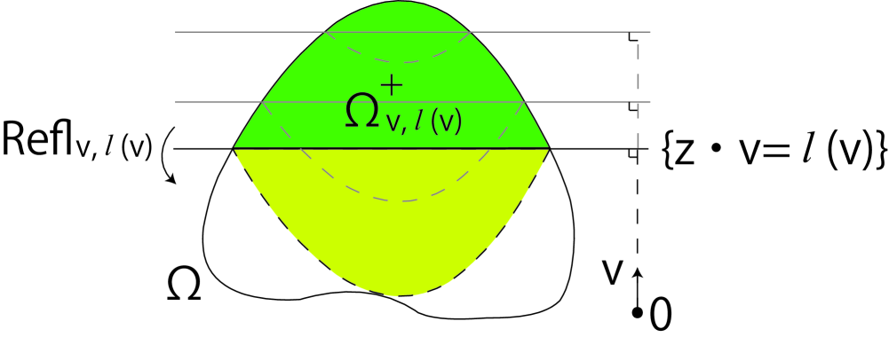
Figure 2: Folding a body $\Omega$ in the manner in Definition 2.21

Example 2.22 ([2, Lemma 5], [17, Example 3.4]).

1. The minimal unfolded region of the disjoint union of three discs is surrounded by the lines through two centers of discs (see Figure 5).

2. The minimal unfolded region of an acute triangle is surrounded by the mid-perpendiculars of edges and the bisectors of angles (see Figure 5).

3. The minimal unfolded region of an obtuse triangle is surrounded by the largest edge, its midperpendicular and the bisectors of angles (see Figure5). We remark that the minimal unfolded region of $\Omega$ is not always contained in the interior of the convex hull of $\Omega$ even if $\Omega$ is convex.

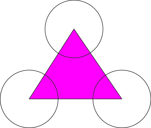
Figure 3: The minimal unfolded region of the disjoint union of three discs

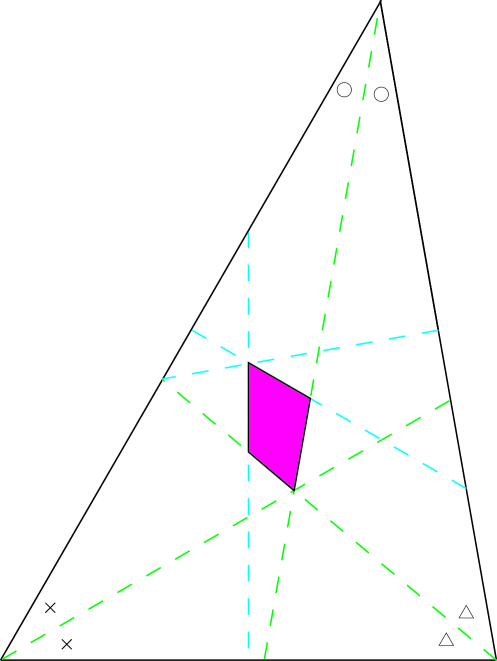
Figure 4: The minimal unfolded region of an acute triangle

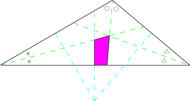
Figure 5: The minimal unfolded region of an obtuse triangle

Remark 2.23 ([2, Proposition 1], [17, p. 381]).

1. The centroid (center of mass) of $\Omega$ is contained in $Uf(\Omega)$. Hence $Uf(\Omega)$ is not empty.

2. $Uf(\Omega)$ is compact and convex.

3. $Uf(\Omega)$ is contained in the convex hull of $\Omega$.

Using the moving plane method ([5, 21]), we can restrict the location of the centers prepared in the previous subsections.

Proposition 2.24.

Let $\Omega$ be a body in $\mathbb{R}^{m}$. For $\alpha\leq 0$, any $r^{\alpha-m}$-center of $\Omega$ belongs to the minimal unfolded region of $\Omega$.

Proof.

Let $x$ be an interior point of $\Omega$ in the complement of the minimal unfolded region of $\Omega$. We show that the point $x$ is not an $r^{\alpha-m}$-center of $\Omega$.

We can choose a direction $v\in S^{m-1}$ with $l(v)<x\cdot v$. Let $b=(l(v)+x\cdot v)/2$. Then, the region $\operatorname{Refl}_{v,b}(\Omega^{+}_{v,b})$ is contained in $\Omega$, and $\Omega\setminus(\Omega^{+}_{v,b}\cup\operatorname{Refl}_{v,b}(\Omega^{+}_{v,b}))$ has an interior point.

Let $x^{\prime}=\operatorname{Refl}_{v,b}(x)$. We choose a small enough $\varepsilon>0$ so that the ball $B_{\varepsilon}(x)$ is contained in the interior of $\Omega$. Then, we have the following properties:

$$\int_{\Omega^{+}_{v,b}\setminus B_{\varepsilon}(x)}\left|x-\xi\right|^{\alpha-m}d\xi =\int_{\operatorname{Refl}_{v,b}\left(\Omega^{+}_{v,b}\right)\setminus B_{\varepsilon}\left(x^{\prime}\right)}\left|x^{\prime}-\xi\right|^{\alpha-m}d\xi,$$

$$\int_{\operatorname{Refl}_{v,b}\left(\Omega^{+}_{v,b}\right)}\left|x-\xi\right|^{\alpha-m}d\xi =\int_{\Omega^{+}_{v,b}}\left|x^{\prime}-\xi\right|^{\alpha-m}d\xi.$$

Furthermore, for any point $\xi\in\Omega\setminus(\Omega^{+}_{v,b}\cup\operatorname{Refl}_{v,b}(\Omega^{+}_{v,b}))$, we have $\left|x-\xi\right|^{\alpha-m}<\left|x^{\prime}-\xi\right|^{\alpha-m}$. Hence, by Proposition 2.7, we obtain

$$V_{\Omega}^{(\alpha)}(x)-V_{\Omega}^{(\alpha)}\left(x^{\prime}\right) =\int_{\Omega\setminus B_{\varepsilon}(x)}\left|x-\xi\right|^{\alpha-m}d\xi-\int_{\Omega\setminus B_{\varepsilon}\left(x^{\prime}\right)}\left|x^{\prime}-\xi\right|^{\alpha-m}d\xi$$

$$=\left(\int_{\Omega^{+}_{v,b}\setminus B_{\varepsilon}(x)}+\int_{\operatorname{Refl}_{v,b}\left(\Omega^{+}_{v,b}\right)}+\int_{\Omega\setminus\left(\Omega^{+}_{v,b}\cup\operatorname{Refl}_{v,b}\left(\Omega^{+}_{v,b}\right)\right)}\right)\left|x-\xi\right|^{\alpha-m}d\xi$$

$$\quad-\left(\int_{\operatorname{Refl}_{v,b}\left(\Omega^{+}_{v,b}\right)\setminus B_{\varepsilon}\left(x^{\prime}\right)}+\int_{\Omega^{+}_{v,b}}+\int_{\Omega\setminus\left(\Omega^{+}_{v,b}\cup\operatorname{Refl}_{v,b}\left(\Omega^{+}_{v,b}\right)\right)}\right)\left|x^{\prime}-\xi\right|^{\alpha-m}d\xi$$

$$<0,$$

which completes the proof. ∎

Remark 2.25.

In [17, Theorem 3.5], O’Hara asserted the same statement as Proposition 2.24 when $\Omega$ has a piecewise $C^{1}$ boundary. But, in this paper, we does not assume the smoothness of a body $\Omega$.

In the same manner as in Proposition 2.24, we can restrict the location of $k$-centers of $\Omega$ into the minimal unfolded region of $\Omega$.

Proposition 2.26 ([19, Proposition 4.9]).

Let $\Omega$ be a body in $\mathbb{R}^{m}$. If $k$ is strictly decreasing and satisfies the condition $(C_{\beta}^{0})$ for some $\beta>0$, then any $k$-center of $\Omega$ belongs to the minimal unfolded region of $\Omega$.

Remark 2.27.

We refer to [8] for the location of $r^{\alpha-m}$-centers. Herburt showed that the (unique) $r^{1-m}$-center of a smooth convex body $A$ belongs to the interior of $A$.

For $\alpha\leq 0$, we discuss the location of $r^{\alpha-m}$-centers in Theorem 3.3 and Corollary 3.4. For $\alpha>1$, any $r^{\alpha-m}$-center of a body $\Omega$ belongs to the intersection $Uf(\Omega)\cap(\operatorname{conv}\Omega)^{\circ}$. This statement follows from the fact that, for a boundary point $x$ of $\operatorname{conv}\Omega$ and the unit outer normal field $n$ of $\operatorname{conv}\Omega$, the derivative

$$\frac{\partial V_{\Omega}^{(\alpha)}}{\partial n(x)}(x)=(\alpha-m)\int_{\Omega}r^{\alpha-m-2}(x-y)\cdot n(x)dy$$

does not vanish.

Herburt’s theorem does not follow from the same argument as in the case of $\alpha>1$. This is because the potential $V_{\Omega}^{(1)}$ is not differentiable at any boundary point of $\Omega$. Also, the minimal unfolded region of $\Omega$ touches the boundary of $\Omega$ in general (see Example 2.22).

Hence, for $0<\alpha<1$, the location of $r^{\alpha-m}$-centers is unknown.

3 Estimation of an $r^{\alpha-m}$-potential

Let $\Omega$ be a body (the closure of a bonded open set) in $\mathbb{R}^{m}$. By Proposition 2.24, the set of $r^{\alpha-m}$-centers ($\alpha\leq 0$) of $\Omega$ is contained in the minimal unfolded region of $\Omega$. But, by Lemma 2.9, it is expected that any $r^{\alpha-m}$-center does not exist “near” the boundary of $\Omega$. For example, when $\Omega$ is an obtuse triangle in $\mathbb{R}^{2}$, the minimal unfolded region of $\Omega$ touches the boundary of $\Omega$, but it is expected that any $r^{\alpha-2}$-center belongs to a smaller closed region contained in the interior of the minimal unfolded region of $\Omega$. Let us show that the expectation is true when the complement of $\Omega$ satisfies the uniform boundary inner cone condition.

Let $C(x)=C(x;\kappa,\delta)$ be an open cone of vertex $x$, axis direction $e_{1}$, aperture angle $0<\kappa\leq\pi$ and height $0<\delta\leq+\infty$, that is,

$$C(x) =C(x;\kappa,\delta)$$

$$=\left.\left\{\rho\left(\begin{array}[]{c}\cos\phi_{1}\\ \sin\phi_{1}\cos\phi_{2}\\ \vdots\\ \sin\phi_{1}\cdots\sin\phi_{m-2}\cos\phi_{m-1}\\ \sin\phi_{1}\cdots\sin\phi_{m-2}\sin\phi_{m-1}\end{array}\right)+x\right|0<\rho<\delta,\ \phi\in\left(-\frac{\kappa}{2},\frac{\kappa}{2}\right)\times[0,\pi]^{m-2}\right\},$$ (3.6)

where $\phi=(\phi_{1},\ldots,\phi_{m-1})$. Let $\operatorname{Rot}_{1m}(\theta)$ denote the rotation in the plane $\operatorname{Span}\langle e_{1},e_{m}\rangle$ of angle $\theta$, that is,

$$\operatorname{Rot}_{1m}(\theta)=\left(\begin{array}[]{ccccc}\cos\theta&&&&-\sin\theta\\ &1&&&\\ &&\ddots&&\\ &&&1&\\ \sin\theta&&&&\cos\theta\end{array}\right).$$ (3.7)

Let

$$C_{\theta}(x)=C_{\theta}(x;\kappa,\delta)=\operatorname{Rot}_{1m}(\theta)C(0;\kappa,\delta)+x.$$ (3.8)

Lemma 3.1.

Let $\alpha\leq 0$, $0<\kappa\leq\pi$, $0<\delta\leq+\infty$, and $0<R<D$. If $\delta\leq D-R$ or $\delta\geq\sqrt{D^{2}-R^{2}}$, then we have

$$\min_{0\leq\theta\leq(\pi-\kappa)/2}\int_{C_{\theta}\left(Re_{1}\right)\cap B_{D}(0)}\left|\xi\right|^{\alpha-m}d\xi=\int_{C\left(Re_{1}\right)\cap B_{D}(0)}\left|\xi\right|^{\alpha-m}d\xi,$$

where $C_{\theta}(Re_{1})=C_{\theta}(Re_{1};\kappa,\delta)$ is the cone defined in (3.8).

Proof.

We take a point $\xi(\theta,\phi)$ from $C_{\theta}(Re_{1})$ as

$$\xi(\theta,\phi)=\rho\left(\begin{array}[]{ccccc}\cos\theta&&&&-\sin\theta\\ &1&&&\\ &&\ddots&&\\ &&&1&\\ \sin\theta&&&&\cos\theta\end{array}\right)\left(\begin{array}[]{c}\cos\phi_{1}\\ \sin\phi_{1}\cos\phi_{2}\\ \vdots\\ \sin\phi_{1}\cdots\sin\phi_{m-2}\cos\phi_{m-1}\\ \sin\phi_{1}\cdots\sin\phi_{m-2}\sin\phi_{m-1}\end{array}\right)+Re_{1}.$$

We remark

$$\left|\xi(\theta,\phi)\right|=\sqrt{\rho^{2}+R^{2}+2\rho R\left(\cos\theta\cos\phi_{1}-\sin\theta\sin\phi_{1}\cdots\sin\phi_{m-2}\sin\phi_{m-1}\right)}.$$

In order to estimate the contribution of a point in the intersection $C_{\theta}(Re_{1})\cap B_{D}(0)$ to the integral, let us show the non-negativity of the difference

$$\Delta(\theta,\phi):=\left|\xi(0,\phi)\right|-\left|\xi(\theta,\phi)\right|-\left|\left|\xi\left(0,\bar{\phi}\right)\right|-\left|\xi\left(\theta,\bar{\phi}\right)\right|\right|$$

for any $0\leq\theta\leq(\pi-\kappa)/2$ and $\phi\in[0,\kappa/2)\times[0,\pi]^{m-2}$ (see Figure 6), where $\bar{\phi}=(\phi_{1},\ldots,\phi_{m-2},-\phi_{m-1})$.

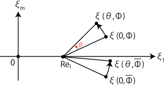
Figure 6: The location of $\xi(\theta,\phi)$ and the difference $\Delta(\theta,\phi)$.

If $\left|\xi(0,\bar{\phi})\right|\geq\left|\xi(\theta,\bar{\phi})\right|$, then we have

$$\Delta(\theta,\phi)=\left|\xi\left(\theta,\bar{\phi}\right)\right|-\left|\xi(\theta,\phi)\right|\geq 0.$$

Let us consider the case of $\left|\xi(0,\bar{\phi})\right|\leq\left|\xi(\theta,\bar{\phi})\right|$. Then we have

$$\Delta(\theta,\phi)=2\left|\xi(0,\phi)\right|-\left|\xi(\theta,\phi)\right|-\left|\xi\left(\theta,\bar{\phi}\right)\right|.$$

It is sufficient to show the non-negativity of the difference

$$4\left|\xi(0,\phi)\right|^{2}-\left(\left|\xi(\theta,\phi)\right|+\left|\xi\left(\theta,\bar{\phi}\right)\right|\right)^{2}.$$

Since we have

$$2\left|\xi(0,\phi)\right|^{2}-\left|\xi(\theta,\phi)\right|^{2}-\left|\xi\left(\theta,\bar{\phi}\right)\right|^{2}=4\rho R\cos\phi_{1}\left(1-\cos\theta\right)\geq 0,$$

we get

$$4\left|\xi(0,\phi)\right|^{2}-\left(\left|\xi(\theta,\phi)\right|+\left|\xi\left(\theta,\bar{\phi}\right)\right|\right)^{2} \geq 2\left|\xi(0,\phi)\right|^{2}-2\left|\xi(\theta,\phi)\right|\left|\xi\left(\theta,\bar{\phi}\right)\right|$$

$$\geq\left|\xi(\theta,\phi)\right|^{2}+\left|\xi\left(\theta,\bar{\phi}\right)\right|^{2}-2\left|\xi(\theta,\phi)\right|\left|\xi\left(\theta,\bar{\phi}\right)\right|$$

$$\geq 0.$$

In order to complete the proof, we prepare the following notation:

$$U_{\theta} =\operatorname{Rot}_{1m}(\theta)\left(C\left(Re_{1}\right)\cap B_{D}(0)\cap\left\{\xi_{m}\geq 0\right\}-Re_{1}\right)+Re_{1},$$

$$L_{\theta} =\operatorname{Rot}_{1m}(\theta)\left(C\left(Re_{1}\right)\cap B_{D}(0)\cap\left\{\xi_{m}\leq 0\right\}-Re_{1}\right)+Re_{1}.$$

The non-negativity of the difference $\Delta(\theta,\phi)$ implies

$$\left(\int_{L_{0}}-\int_{L_{\theta}}\right)\left|\xi\right|^{\alpha-m}d\xi\leq\left(\int_{U_{\theta}}-\int_{U_{0}}\right)\left|\xi\right|^{\alpha-m}d\xi,$$

and hence, we get

$$\int_{C\left(Re_{1}\right)\cap B_{D}(0)}\left|\xi\right|^{\alpha-m}d\xi=\int_{U_{0}\cup L_{0}}\left|\xi\right|^{\alpha-m}d\xi\leq\int_{U_{\theta}\cup L_{\theta}}\left|\xi\right|^{\alpha-m}d\xi.$$

If $\delta\leq D-R$, then $C_{\theta}(Re_{1})=C_{\theta}(Re_{1})\cap B_{D}(0)=U_{\theta}\cup L_{\theta}$, that is, the proof is completed in this case. Let us consider the case of $\delta\geq\sqrt{D^{2}-R^{2}}$. Using the non-negativity of $\Delta(\theta,\phi)$, we can show

$$\operatorname{Vol}\left(\left(U_{\theta}\cup L_{\theta}\right)\setminus\left(C_{\theta}\left(Re_{1}\right)\cap B_{D}(0)\right)\right)\leq\operatorname{Vol}\left(\left(C_{\theta}\left(Re_{1}\right)\cap B_{D}(0)\right)\setminus\left(U_{\theta}\cup L_{\theta}\right)\right)$$

(see Figure 7). Hence we obtain

$$\int_{U_{\theta}\cup L_{\theta}}\left|\xi\right|^{\alpha-m}d\xi\leq\int_{C_{\theta}\left(Re_{1}\right)\cap B_{D}(0)}\left|\xi\right|^{\alpha-m}d\xi,$$

which completes the proof .

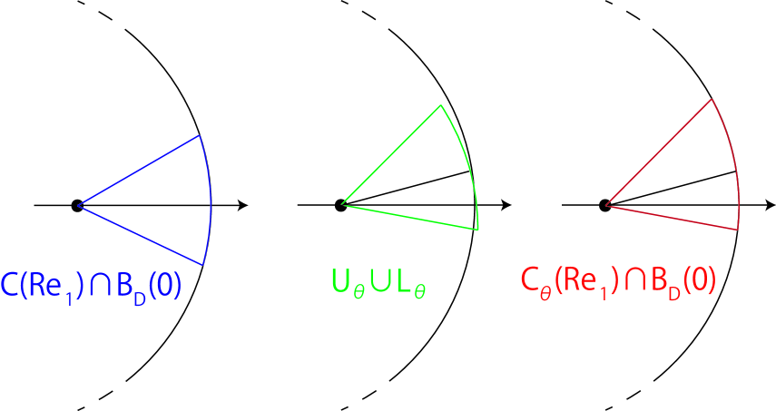
Figure 7: The estimation of the integrals

∎

Lemma 3.2.

Let $\alpha\leq 0$, $0<\kappa\leq\pi$, $0<\delta\leq+\infty$, $D>0$, and $0<R_{0}<D$. Define the function

$$E(R)=E\left(R;\alpha,\kappa,\delta,D,R_{0}\right)=\min_{0\leq\theta\leq(\pi-\kappa)/2}\left(\int_{C_{\theta}\left(Re_{1}\right)\cap B_{D}(0)}-\int_{B_{D}(0)\setminus B_{R_{0}}(0)}\right)\left|\xi\right|^{\alpha-m}d\xi,\ R>0,$$

where $C_{\theta}(Re_{1})=C_{\theta}(Re_{1};\kappa,\delta)$ is the cone defined in (3.8).

1. The function $E$ is strictly decreasing.

2. There exists a unique positive constant $\tilde{R}=\tilde{R}(\alpha,\kappa,\delta,D,R_{0})$ such that $E(R)>0$ if $R<\tilde{R}$, and that $E(R)<0$ if $R>\tilde{R}$. In particular, $\tilde{R}$ is the unique zero point of $E$.

3. The unique zero point $\tilde{R}$ is less than $R_{0}$.

Proof.

(1) Let $0<R_{1}<R_{2}$. We denote by $\theta_{j}$ an angle giving the minimum value in the definition of $E(R_{j})$. The strictly decreasing behavior of the function $r\mapsto r^{\alpha-m}$ implies

$$E\left(R_{1}\right) =\left(\int_{C_{\theta_{1}}\left(R_{1}e_{1}\right)\cap B_{D}(0)}-\int_{B_{D}(0)\setminus B_{R_{0}}(0)}\right)\left|\xi\right|^{\alpha-m}d\xi$$

$$>\left(\int_{C_{\theta_{1}}\left(R_{2}e_{1}\right)\cap B_{D}(0)}-\int_{B_{D}(0)\setminus B_{R_{0}}(0)}\right)\left|\xi\right|^{\alpha-m}d\xi$$

$$\geq\left(\int_{C_{\theta_{2}}\left(R_{2}e_{1}\right)\cap B_{D}(0)}-\int_{B_{D}(0)\setminus B_{R_{0}}(0)}\right)\left|\xi\right|^{\alpha-m}d\xi$$

$$=E\left(R_{2}\right).$$

(2) First, we remark that $E(R)$ is negative for $R\geq R_{0}$. This is because, for any $0\leq\theta\leq(\pi-\kappa)/2$ and $R\geq R_{0}$, $C_{\theta}\left(Re_{1}\right)\cap B_{D}(0)$ is contained in the annulus $B_{D}(0)\setminus B_{R_{0}}(0)$.

Next, we show that $E(R)$ diverges to $+\infty$ as $R\to 0^{+}$. We take a small enough $\varepsilon>0$ so that $\varepsilon\delta<D-R_{0}$. Then, for any $0\leq\theta\leq(\pi-\kappa)/2$ and $R\leq R_{0}$, the small cone $\varepsilon C_{\theta}(Re_{1})$ is contained in the ball $B_{D}(0)$. From Lemma 3.1, we have

$$\min_{0\leq\theta\leq(\pi-\kappa)/2}\int_{\varepsilon C_{\theta}\left(Re_{1}\right)\cap B_{D}(0)}\left|\xi\right|^{\alpha-m}d\xi=\int_{\varepsilon C\left(Re_{1}\right)\cap B_{D}(0)}\left|\xi\right|^{\alpha-m}d\xi.$$

Therefore, Lemma 2.9 implies

$$E(R)\geq\left(\int_{\varepsilon C\left(Re_{1}\right)\cap B_{D}(0)}-\int_{B_{D}(0)\setminus B_{R_{0}}(0)}\right)\left|\xi\right|^{\alpha-m}d\xi\to+\infty$$

as $R\to 0^{+}$.

Hence the continuity of $E$ implies the existence and uniqueness of a zero point of $E$.

(3) The statement was shown in the proof of (2) as $E(R)$ is negative for $R\geq R_{0}$. ∎

Theorem 3.3.

Let $\alpha\leq 0$. Let $X$ and $Y$ be bodies in $\mathbb{R}^{m}$. Suppose that the complement of $Y$ satisfies the uniform boundary inner cone condition of aperture angle $\kappa$ and height $\delta$. Let $R_{0}>0$, and $\tilde{R}=\tilde{R}(\alpha,\kappa,\delta,\operatorname{diam}Y,R_{0})$ be as in Lemma 3.2. For any points $x\in X$ with $\operatorname{dist}(x,X^{c})\geq R_{0}$ and $y\in Y$ with $\operatorname{dist}(y,Y^{c})\leq\tilde{R}$, we have $V_{Y}^{(\alpha)}(y)<V_{X}^{(\alpha)}(x)$.

Proof.

If $R_{0}$ is greater than half of the diameter of $Y$, then the statement obviously hods. Let us consider the case where $R_{0}$ is not greater than half of the diameter of $Y$.

Fix an interior point $y$ of $Y$. Let $y^{\prime}$ be a boundary point of $Y$ with $|y-y^{\prime}|=\operatorname{dist}(y,Y^{c})$. From the uniform boundary inner cone condition of the complement of $Y$, there is a direction $v(y)$ such that we can take an open cone of vertex $y^{\prime}$, axis direction $v(y)$, aperture angle $\kappa$ and height $\delta$. Let $\theta(y)$ be the angle between $(y^{\prime}-y)/|y^{\prime}-y|$ and $v(y)$. By radial symmetry of the kernel of $V_{Y}^{(\alpha)}$, we get

$$V_{Y}^{(\alpha)}(y)<V_{B_{\operatorname{diam}Y}(0)\setminus C_{\theta(y)}\left(\operatorname{dist}\left(y,Y^{c}\right)e_{1}\right)}^{(\alpha)}(0),$$

where $C_{\theta(y)}\left(\operatorname{dist}\left(y,Y^{c}\right)e_{1}\right)=C_{\theta(y)}\left(\operatorname{dist}\left(y,Y^{c}\right)e_{1};\kappa,\delta\right)$ is the cone defined in (3.8). Also, we have

$$V_{X}^{(\alpha)}(x)\geq V_{B_{R_{0}}(0)}^{(\alpha)}(0).$$

Hence, for any points $x\in X$ with $\operatorname{dist}(x,X^{c})\geq R_{0}$ and $y\in Y$ with $\operatorname{dist}(y,Y^{c})\leq\tilde{R}$, we get

$$V_{X}^{(\alpha)}(x)-V_{Y}^{(\alpha)}(y) >V_{B_{R_{0}}(0)}^{(\alpha)}(0)-V_{B_{\operatorname{diam}Y}(0)\setminus C_{\theta(y)}\left(\operatorname{dist}\left(y,Y^{c}\right)e_{1}\right)}^{(\alpha)}(0)$$

$$=\left(\int_{C_{\theta(y)}\left(\operatorname{dist}\left(y,Y^{c}\right)e_{1}\right)\cap B_{\operatorname{diam}Y}(0)}-\int_{B_{\operatorname{diam}Y}(0)\setminus B_{R_{0}}(0)}\right)\left|\xi\right|^{\alpha-m}d\xi$$

$$\geq E\left(\operatorname{dist}\left(y,Y^{c}\right)\right)$$

$$\geq 0,$$

where $E=E(\cdot;\alpha,\kappa,\delta,\operatorname{diam}Y,R_{0})$ is defined in Lemma 3.2. ∎

Corollary 3.4.

Let $\alpha\leq 0$. Let $\Omega$ be a body in $\mathbb{R}^{m}$ whose complement satisfies the uniform boundary inner cone condition of aperture angle $\kappa$ and height $\delta$. Any $r^{\alpha-m}$-center of $\Omega$ belongs to the intersection $(\Omega\sim\tilde{R}B^{m})\cap Uf(\Omega)$, where $\tilde{R}=\tilde{R}(\alpha,\kappa,\delta,\operatorname{diam}\Omega,R_{\infty}(\Omega))$ is given in Lemma 3.2.

Example 3.5.

Let $\alpha\leq 0$. For $0\leq\varepsilon\leq 1$, let

$$\Omega_{\varepsilon}=\left([-3,-1]\times B^{m-1}\right)\cup\left([-1,1]\times\varepsilon B^{m-1}\right)\cup\left([1,3]\times B^{m-1}\right).$$

We take an open cone $C$ of aperture angle $\kappa$ and height $\delta$ such that the complement of $\Omega_{0}$ satisfies the uniform interior cone condition for $C$. Then, for any $0<\varepsilon\leq 1$, the complement of the body $\Omega_{\varepsilon}$ satisfies the uniform interior cone condition for $C$. We remark $\operatorname{diam}\Omega_{\varepsilon}=2\sqrt{10}$ and $R_{\infty}(\Omega_{\varepsilon})=1$ for any $0\leq\varepsilon\leq 1$. Let $\tilde{R}=\tilde{R}(\alpha,\kappa,\delta,3\sqrt{5},1)$ be as in Lemma 3.2, and fix an $0<\varepsilon<\tilde{R}$.

Since $Uf(\Omega)=[-2,2]\times\{0\}^{m-1}$ and $\tilde{R}<1$, Corollary 3.4 implies that any $r^{\alpha-m}$-center of the body $\Omega_{\varepsilon}$ belongs to the disjoint union of the intervals $([-2,-1-\sqrt{\tilde{R}^{2}-\varepsilon^{2}}]\cup[1+\sqrt{\tilde{R}^{2}-\varepsilon^{2}},2])\times\{0\}^{m-1}$. Radial symmetry of the kernel of $V_{\Omega_{\varepsilon}}^{(\alpha)}$ guarantees that each interval has an $r^{\alpha-m}$-center. In particular, the potential $V_{\Omega_{\varepsilon}}^{(\alpha)}$ has at least two maximizers.

Example 3.6.

Let $\alpha\leq 0$, and $\Omega=B_{3}(0)\setminus\overset{\mbox{\tiny$\circ$}}{B}_{1}(0)$. We take an open cone $C$ of aperture angle $\kappa$ and height $\delta$ such that the complement of $\Omega$ satisfies the uniform boundary inner cone condition for $C$. We remark $\operatorname{diam}\Omega=6$ and $R_{\infty}(\Omega)=1$. Let $\tilde{R}=\tilde{R}(\alpha,\kappa,\delta,6,1)$ be as in Lemma 3.2.

Since $Uf(\Omega)=B_{2}(0)$ and $\tilde{R}<1$, Corollary 3.4 implies that any $r^{\alpha-m}$-center belongs to the annulus $B_{2}(0)\setminus\overset{\mbox{\tiny$\circ$}}{B}_{1+\tilde{R}}(0)$. Radial symmetry of the kernel of $V_{\Omega}^{(\alpha)}$ guarantees the existence of a positive constant $1+\tilde{R}\leq\rho\leq 2$ such that the set of $r^{\alpha-m}$-centers contains the sphere $\rho S^{m-1}$.

4 Estimation of a potential with a summable kernel

Let $\Omega$ be a body (the closure of a bounded open set) in $\mathbb{R}^{m}$. In this section, we estimate a potential of the form

$$K_{\Omega}^{(\alpha)}(x,t)=\int_{\Omega}k_{\alpha}\left(\left|x-\xi\right|,t\right)d\xi,\ x\in\mathbb{R}^{m},\ t>0.$$ (4.1)

Assumption 4.1.

For the kernel $k_{\alpha}$ in (4.1), we assume some or all of the following conditions:

1. $k_{\alpha}(\cdot,t)$ is strictly decreasing and satisfies the condition $(C^{0}_{\beta})$ for some $\beta>0$.

2. We can choose a pair of positive functions $(\psi,\bar{k}_{\alpha})$ such that the kernel $k_{\alpha}$ is expressed as $k(r,t)=\psi(t)\bar{k}_{\alpha}(r,t)$, and that $\bar{k}_{\alpha}(r,t)$ converges to $r^{\alpha-m}$ for each positive $r$ as $t$ tends to $0^{+}$.

3. For each positive $t$, we have

   $$\int_{\mathbb{R}^{m}}k_{\alpha}\left(\left|\xi\right|,t\right)d\xi=1.$$

4. For any positive $\rho$, we have

   $$\lim_{t\to 0^{+}}\int_{\mathbb{R}^{m}\setminus B_{\rho}(0)}k_{\alpha}\left(\left|\xi\right|,t\right)d\xi=0.$$

Usually, a radially symmetric non-negative kernel is said to be summable if it satisfies the conditions (3) and (4).

Lemma 4.2.

Let $\alpha\leq 0$. Suppose that $k_{\alpha}$ satisfies the conditions $(1)$ and $(2)$ in Assumption 4.1. Let $X$ and $Y$ be bodies in $\mathbb{R}^{m}$. Suppose that the complement of $Y$ satisfies the uniform boundary inner cone condition of aperture angle $\kappa$ and height $\delta$. Let $R_{0}>0$, and $\tilde{R}=\tilde{R}(\alpha,\kappa,\delta,\operatorname{diam}Y,R_{0})$ be given in Lemma 3.2. For any $0<b<1$, there exists a positive $\tau_{1}$ such that if $0<t<\tau_{1}$, then, for any $x\in X$ with $\operatorname{dist}(x,X^{c})\geq R_{0}$ and $y\in Y$ with $(b/2)\tilde{R}\leq\operatorname{dist}(y,Y^{c})\leq b\tilde{R}$, we have $K_{Y}^{(\alpha)}(y,t)<K_{X}^{(\alpha)}(x,t)$.

Proof.

If $R_{0}$ is greater than half of the diameter of $Y$, then the statement obviously holds. Let us assume that $R_{0}$ is not greater than half of the diameter of $Y$.

Thanks to the uniform boundary inner cone condition of the complement of $Y$, in the same manner as in Theorem 3.3, for any point $y\in Y$, we can choose a constant $0\leq\theta(y)\leq(\pi-\kappa)/2$ such that, for each $t$, we have

$$K_{Y}^{(\alpha)}(y,t)<K_{B_{\operatorname{diam}Y}(0)\setminus C_{\theta(y)}\left(\operatorname{dist}\left(y,Y^{c}\right)e_{1}\right)}^{(\alpha)}(0),$$

where $C_{\theta(y)}\left(\operatorname{dist}(y,Y^{c})e_{1}\right)=C_{\theta(y)}\left(\operatorname{dist}(y,Y^{c})e_{1};\kappa,\delta\right)$ is the cone defined in (3.8).

By the assumption for the kernel $k_{\alpha}$ and the compactness of the body $Y$, there exits a positive constant $\tau_{1}$ such that if $0<t<\tau_{1}$, then, for any $\xi\in(C((b/2)\tilde{R}e_{1};\pi,+\infty)\cap B_{\operatorname{diam}Y}(0))\cup(B_{\operatorname{diam}Y}(0)\setminus B_{R_{0}}(0))$, we have

$$\left|k_{\alpha}\left(\left|\xi\right|,t\right)-\left|\xi\right|^{\alpha-m}\right|$$

$$<\frac{E\left(b\tilde{R}\right)}{2\left(\operatorname{Vol}\left(C\left(\frac{b}{2}\tilde{R}e_{1};\pi,+\infty\right)\cap B_{\operatorname{diam}Y}(0)\right)+\operatorname{Vol}\left(B_{\operatorname{diam}Y}(0)\setminus B_{R_{0}}(0)\right)\right)},$$

where $E=E(\cdot;\alpha,\kappa,\delta,\operatorname{diam}Y,R_{0})$ is defined in Lemma 3.2. Since, for any $y\in Y$ with $(b/2)\tilde{R}\leq\operatorname{dist}(y,Y^{c})$, the cone $C_{\theta(y)}(\operatorname{dist}(y,Y^{c})e_{1})$ is contained in the half space $C((b/2)\tilde{R}e_{1};\pi,+\infty)$, we obtain

$$\left|\left(\int_{C_{\theta(y)}\left(\operatorname{dist}\left(y,Y^{c}\right)e_{1}\right)\cap B_{\operatorname{diam}Y}(0)}-\int_{B_{\operatorname{diam}Y}(0)\setminus B_{R_{0}}(0)}\right)\left(\bar{k}_{\alpha}\left(\left|\xi\right|,t\right)-\left|\xi\right|^{\alpha-m}\right)d\xi\right|$$

$$\leq\left(\int_{C_{\theta(y)}\left(\operatorname{dist}\left(y,Y^{c}\right)e_{1}\right)\cap B_{\operatorname{diam}Y}(0)}+\int_{B_{\operatorname{diam}Y}(0)\setminus B_{R_{0}}(0)}\right)\left|\bar{k}_{\alpha}\left(\left|\xi\right|,t\right)-\left|\xi\right|^{\alpha-m}\right|d\xi$$

$$<\frac{1}{2}E\left(b\tilde{R}\right),$$

for any $y\in Y$ with $(b/2)\tilde{R}\leq\operatorname{dist}(y,Y^{c})$.

Hence if $0<t<\tau_{1}$, then, for any $x\in X$ with $\operatorname{dist}(x,X^{c})\geq R_{0}$ and $y\in Y$ with $(b/2)\tilde{R}\leq\operatorname{dist}(y,Y^{c})\leq b\tilde{R}$, we obtain

$$\frac{K_{X}^{(\alpha)}(x,t)-K_{Y}^{(\alpha)}(y,t)}{\psi(t)}$$

$$>\left(\int_{C_{\theta(y)}\left(\operatorname{dist}\left(y,Y^{c}\right)e_{1}\right)\cap B_{\operatorname{diam}Y}(0)}-\int_{B_{\operatorname{diam}Y}(0)\setminus B_{R_{0}}(0)}\right)\bar{k}_{\alpha}\left(\left|\xi\right|,t\right)d\xi$$

$$>\left(\int_{C_{\theta(y)}\left(\operatorname{dist}\left(y,Y^{c}\right)e_{1}\right)\cap B_{\operatorname{diam}Y}(0)}-\int_{B_{\operatorname{diam}Y}(0)\setminus B_{R_{0}}(0)}\right)\left|\xi\right|^{\alpha-m}d\xi-\frac{1}{2}E\left(b\tilde{R}\right)$$

$$\geq E\left(\operatorname{dist}\left(y,Y^{c}\right)\right)-\frac{1}{2}E\left(b\tilde{R}\right)$$

$$\geq\frac{1}{2}E\left(b\tilde{R}\right)$$

$$>0,$$

where the forth inequality follows from the first assertion in Lemma 3.2. ∎

Lemma 4.3.

Let $\alpha$, $k_{\alpha}$, $X$, $Y$, $R_{0}$, $\tilde{R}$, $b$ and $\tau_{1}$ be as in Lemma 4.2. If $0<t<\tau_{1}$, then, for any $x\in X$ with $\operatorname{dist}(x,X^{c})\geq R_{0}$ and $y\in Y$ with $\operatorname{dist}(y,Y^{c})\leq(b/2)\tilde{R}$, we have $K_{Y}^{(\alpha)}(y,t)<K_{X}^{(\alpha)}(x,t)$.

Proof.

For any $0\leq\theta\leq(\pi-\kappa)/2$ and $0\leq R\leq(b/2)\tilde{R}$, the strictly decreasing behavior of $k_{\alpha}(\cdot,t)$ implies

$$\left(\int_{C_{\theta}\left(Re_{1}\right)\cap B_{\operatorname{diam}Y}(0)}-\int_{B_{\operatorname{diam}Y}(0)\setminus B_{R_{0}}(0)}\right)k_{\alpha}\left(\left|\xi\right|,t\right)d\xi$$

$$>\left(\int_{C_{\theta}\left(\left(R+(b/2)\tilde{R}\right)e_{1}\right)\cap B_{\operatorname{diam}Y}(0)}-\int_{B_{\operatorname{diam}Y}(0)\setminus B_{R_{0}}(0)}\right)k_{\alpha}\left(\left|\xi\right|,t\right)d\xi$$

$$\geq\frac{\psi(t)}{2}E\left(b\tilde{R}\right),$$

where the last inequality was shown in Lemma 4.2. This inequality implies the conclusion in the same manner as in Lemma 4.2. ∎

Proposition 4.4.

Let $\alpha$, $k_{\alpha}$, $X$, $Y$, $R_{0}$, $\tilde{R}$, $b$ and $\tau_{1}$ be as in Lemma 4.2. If $0<t<\tau_{1}$, then, for any $x\in X$ with $\operatorname{dist}(x,X^{c})\geq R_{0}$ and $y\in Y$ with $\operatorname{dist}(y,Y^{c})\leq b\tilde{R}$, we have $K_{Y}^{(\alpha)}(y,t)<K_{X}^{(\alpha)}(x,t)$.

Lemma 4.5.

Suppose that $k_{\alpha}$ satisfies the conditions $(3)$ and $(4)$ in Assumption 4.1. Let $C_{\theta}(x;\kappa,\delta)$ be the cone defined in (3.8). For any $\theta$, we have

$$\lim_{t\to 0^{+}}\int_{C_{\theta}(0;\kappa,\delta)}k_{\alpha}\left(\left|\xi\right|,t\right)d\xi=\frac{\sigma\left(C(0;\kappa,1)\cap S^{m-1}\right)}{\sigma\left(S^{m-1}\right)}.$$

Proof.

We remark that the conditions (3) and (4) imply

$$\lim_{t\to 0^{+}}\int_{B_{\delta}(0)}k_{\alpha}\left(\left|\xi\right|,t\right)d\xi=\lim_{t\to 0^{+}}\left(\int_{\mathbb{R}^{m}}-\int_{\mathbb{R}^{m}\setminus B_{\delta}(0)}\right)k_{\alpha}\left(\left|\xi\right|,t\right)d\xi=1.$$

Since we have

$$\operatorname{Vol}\left(C_{\theta}\left(0;\kappa,\delta\right)\right)=\frac{\sigma\left(C(0;\kappa,1)\cap S^{m-1}\right)}{\sigma\left(S^{m-1}\right)}\operatorname{Vol}\left(B_{\delta}(0)\right),$$

the rotation invariance of our potential implies

$$\int_{C_{\theta}(0;\kappa,\delta)}k_{\alpha}\left(\left|\xi\right|,t\right)d\xi=\frac{\sigma\left(C(0;\kappa,1)\cap S^{m-1}\right)}{\sigma\left(S^{m-1}\right)}\int_{B_{\delta}(0)}k_{\alpha}\left(\left|\xi\right|,t\right)d\xi\to\frac{\sigma\left(C(0;\kappa,1)\cap S^{m-1}\right)}{\sigma\left(S^{m-1}\right)}$$

as $t$ tends to $0^{+}$. ∎

Proposition 4.6.

Suppose that $k_{\alpha}$ satisfies the conditions $(3)$ and $(4)$ in Assumption 4.1. Let $X$ and $Y$ be bodies in $\mathbb{R}^{m}$. Suppose that the complement of $Y$ satisfies the uniform interior cone condition of aperture angle $\kappa$ and height $\delta$. Let $R_{0}>0$. There exists a positive $\tau_{2}$ such that if $0<t<\tau_{2}$, then, for any $x\in X$ with $\operatorname{dist}(x,X^{c})\geq R_{0}$ and $y\in Y^{c}$, we have $K_{Y}^{(\alpha)}(y,t)<K_{X}^{(\alpha)}(x,t)$.

Proof.

By the conditions (3) and (4) for the kernel, we can choose a positive constant $\tau_{21}$ such that if $0<t<\tau_{21}$, then, for any point $x\in X$ with $\operatorname{dist}(x,X^{c})\geq R_{0}$, we have

$$K_{X}^{(\alpha)}(x,t)\geq K_{B_{R_{0}}(0)}^{(\alpha)}(0,t)>1-\frac{\sigma\left(C(0;\kappa,1)\cap S^{m-1}\right)}{2\sigma\left(S^{m-1}\right)},$$

where the cone $C(0;\kappa,1)$ is defined in (3.6).

On the other hand, we can choose a positive constant $\tau_{22}$ such that if $0<t<\tau_{22}$, then, for any $y\in Y^{c}$, the uniform interior cone condition of $Y^{c}$ and Lemma 4.5 imply

$$K_{Y}^{(\alpha)}(y,t)\leq K_{\mathbb{R}^{m}\setminus C(0)}^{(\alpha)}(0,t)=1-K_{C(0)}^{(\alpha)}(0,t)<1-\frac{\sigma\left(C(0;\kappa,1)\cap S^{m-1}\right)}{2\sigma\left(S^{m-1}\right)}.$$

Taking $\tau_{2}=\min\{\tau_{21},\ \tau_{22}\}$, the proof is completed. ∎

Theorem 4.7.

Let $\alpha\leq 0$. Suppose that $k_{\alpha}$ satisfies all the conditions in Assumption 4.1. Let $X$ and $Y$ be bodies in $\mathbb{R}^{m}$. Suppose that the complement of $Y$ satisfies the uniform interior cone condition of aperture angle $\kappa$ and height $\delta$. Let $R_{0}>0$, and $\tilde{R}=\tilde{R}(\alpha,\kappa,\delta,\operatorname{diam}Y,R_{0})$ be given in Lemma 3.2. For any $0<b<1$, there exists a positive $\tau$ such that if $0<t<\tau$, then, for any $x\in X$ with $\operatorname{dist}(x,X^{c})\geq R_{0}$ and $y\in\mathbb{R}^{m}$ with $\operatorname{dist}(y,Y^{c})\leq b\tilde{R}$, we have $K_{Y}^{(\alpha)}(y,t)<K_{X}^{(\alpha)}(x,t)$.

Proof.

Thanks to Lemma 2.3, the complement of $Y$ satisfies the uniform boundary inner cone condition of aperture angle $\kappa$ and height $\delta$. Let $\tau_{1}$ and $\tau_{2}$ be as in Propositions 4.4 and 4.6, respectively. Taking $\tau=\min\{\tau_{1},\ \tau_{2}\}$, we obtain the conclusion. ∎

Corollary 4.8.

Let $\alpha\leq 0$ and $k_{\alpha}$ be as in Theorem 4.7. Let $\Omega$ be a body in $\mathbb{R}^{m}$ whose complement satisfies the uniform interior cone condition of aperture angle $\kappa$ and height $\delta$. Let $\tilde{R}=\tilde{R}(\alpha,\kappa,\delta,\operatorname{diam}\Omega,R_{\infty}(\Omega))$ be given in Lemma 3.2. For any $0<b<1$, there exits a positive constant $\tau$ such that if $0<t<\tau$, then any $k_{\alpha}$-center of $\Omega$ at time $t$ is contained in the intersection $(\Omega\sim b\tilde{R}B^{m})\cap Uf(\Omega)$.

Proof.

Thanks to Proposition 2.26, all the $k_{\alpha}$-centers are contained in the minimal unfolded region of $\Omega$. Hence, combining Theorem 4.7, we obtain the conclusion. ∎

Example 4.9.

Let $\alpha\leq 0$. Suppose that $k_{\alpha}$ satisfies all the conditions in Assumption 4.1. Let $\varepsilon$, $\Omega_{\varepsilon}$, $C$ and $\tilde{R}$ be as in Example 3.5. Fix an $0<\varepsilon<\tilde{R}$.

Corollary 4.8 guarantees the existence of a positive constant $\tau$ such that if $0<t<\tau$, then any $k_{\alpha}$-center of the body $\Omega_{\varepsilon}$ at time $t$ belongs to the disjoint union of the intervals $([-2,-1-\sqrt{\tilde{R}^{2}-\varepsilon^{2}}]\cup[1+\sqrt{\tilde{R}^{2}-\varepsilon^{2}},2])\times\{0\}^{m-1}$. Radial symmetry of the kernel of $K_{\Omega_{\varepsilon}}^{(\alpha)}(\cdot,t)$ guarantees that each interval has an $k_{\alpha}$-center. In particular, the potential $K_{\Omega_{\varepsilon}}^{(\alpha)}(\cdot,t)$ has at least two maximizers for any sufficiently small $t$.

Example 4.10.

Let $\alpha\leq 0$. Suppose that $k_{\alpha}$ satisfies all the conditions in Assumption 4.1. Let $\Omega$, $C$ and $\tilde{R}$ be as in Example 3.6.

Corollary 4.8 guarantees the existence of a positive constant $\tau$ such that if $0<t<\tau$, then any $k_{\alpha}$-center of $\Omega$ at time $t$ belongs to the annulus $B_{2}(0)\setminus\overset{\mbox{\tiny$\circ$}}{B}_{1+\tilde{R}}(0)$. Radial symmetry of the kernel of $K_{\Omega}^{(\alpha)}(\cdot,t)$ guarantees the existence of a positive constant $1+\tilde{R}\leq\rho(t)\leq 2$ such that the set of $k_{\alpha}$-centers of $\Omega$ at time $t$ contains the sphere $\rho(t)S^{m-1}$ for any sufficiently small $t$.

Corollary 4.11.

Let $\alpha\leq 0$ and $k_{\alpha}$ be as in Theorem 4.7. Let $\Omega$ be a convex body in $\mathbb{R}^{m}$. Let $\tilde{R}=\tilde{R}(\alpha,\pi,+\infty,\operatorname{diam}\Omega,R_{\infty}(\Omega))$ be given in Lemma 3.2. Let $0<b<1$, and $\Omega^{\prime}=(\Omega\sim b\tilde{R}B^{m})\cap Uf(\Omega)$. Suppose the existence of a positive constant $\tau^{\prime}$ such that, for any $0<t<\tau^{\prime}$, $k_{\alpha}(r,t)r^{m-1}$ is decreasing on the interval $[d(\Omega,\Omega^{\prime}),D(\Omega,\Omega^{\prime})]$ with respect to $r$. There exists a positive constant $\tau\leq\tau^{\prime}$ such that, for any $0<t<\tau$, $K_{\Omega}^{(\alpha)}(\cdot,t)$ is strictly concave on $\Omega^{\prime}$. In particular, $\Omega$ has a unique $k_{\alpha}$-center at time $0<t<\tau$.

Proof.

Since $(\Omega\sim b\tilde{R}B^{m})\cap Uf(\Omega)$ is convex and contained in the interior of $\Omega$, Propositions 2.20 guarantees the conclusion. ∎

Theorem 4.12.

Let $\alpha\leq 0$. Suppose that $k_{\alpha}$ satisfies all the conditions in Assumption 4.1. Let $\Omega$ be a body in $\mathbb{R}^{m}$ whose complement satisfies the uniform interior cone condition of aperture angle $\kappa$ and height $\delta$. For any decreasing sequence $\{t_{\ell}\}$ with zero limiting value and any $k_{\alpha}$-center $c_{\alpha}(t_{\ell})$ at time $t_{\ell}$, the distance between $c_{\alpha}(t_{\ell})$ and the set of $r^{\alpha-m}$-centers tends to zero as $\ell$ goes to $+\infty$.

Proof.

Thanks to Corollary 4.8, we may assume that any $k_{\alpha}$-center at time $t_{\ell}$ belongs to the inner-parallel body of $\Omega$ of radius $(1/2)\tilde{R}$, where $\tilde{R}=\tilde{R}(\alpha,\kappa,\delta,\operatorname{diam}\Omega,R_{\infty}(\Omega))$ is given in Lemma 3.2. Since the inner-parallel body is compact, without loss of generality, we assume that $\{c_{\alpha}(t_{\ell})\}$ converges to a point $c_{\alpha}$. In order to show that $c_{\alpha}$ is an $r^{\alpha-m}$-center of $\Omega$, we assume that $c_{\alpha}$ is not any $r^{\alpha-m}$-center, and let us derive a contradiction.

Fix an arbitrary $0<\varepsilon<(1/2)\tilde{R}$. Then, for any point $x$ in the inner-parallel body of $\Omega$ of radius $(1/2)\tilde{R}$, we have

$$K_{\Omega}^{(\alpha)}(x,t) =\left(\int_{\Omega\setminus B_{\varepsilon}(x)}+\int_{B_{\varepsilon}(x)}\right)k_{\alpha}\left(\left|x-\xi\right|,t\right)d\xi$$

$$=\int_{\Omega\setminus B_{\varepsilon}(x)}k_{\alpha}\left(\left|x-\xi\right|,t\right)d\xi+\sigma\left(S^{m-1}\right)\int_{0}^{\varepsilon}k_{\alpha}\left(r,t\right)r^{m-1}dr.$$

Therefore, the maximum value of $K_{\Omega}^{(\alpha)}(\cdot,t_{\ell})$ is attained at $c_{\alpha}(t_{\ell})$ if and only if that of the function

$$\Omega\sim\frac{1}{2}\tilde{R}B^{m}\ni x\mapsto\int_{\Omega\setminus B_{\varepsilon}(x)}\bar{k}_{\alpha}\left(\left|x-\xi\right|,t_{\ell}\right)d\xi\in\mathbb{R}$$

is attained at $c_{\alpha}(t_{\ell})$.

Let $p$ be an $r^{\alpha-m}$-center of $\Omega$. Thanks to the first and second conditions in Assumption 4.1, there exists a large natural number $L$ such that, for any $\ell\geq L$, the following inequalities hold:

$$\left|\int_{\Omega\setminus B_{\varepsilon}\left(c_{\alpha}\left(t_{\ell}\right)\right)}\bar{k}_{\alpha}\left(\left|c_{\alpha}\left(t_{\ell}\right)-\xi\right|,t_{\ell}\right)d\xi-\int_{\Omega\setminus B_{\varepsilon}\left(c_{\alpha}\right)}\left|c_{\alpha}-\xi\right|^{\alpha-m}d\xi\right|\leq\frac{V_{\Omega}^{(\alpha)}(p)-V_{\Omega}^{(\alpha)}\left(c_{\alpha}\right)}{3},$$

$$\left|\int_{\Omega\setminus B_{\varepsilon}(p)}\bar{k}_{\alpha}\left(\left|p-\xi\right|,t_{\ell}\right)d\xi-\int_{\Omega\setminus B_{\varepsilon}(p)}\left|p-\xi\right|^{\alpha-m}d\xi\right|\leq\frac{V_{\Omega}^{(\alpha)}(p)-V_{\Omega}^{(\alpha)}\left(c_{\alpha}\right)}{3}.$$

Hence, using Proposition 2.7, we obtain

$$0 \leq\int_{\Omega\setminus B_{\varepsilon}\left(c_{\alpha}\left(t_{\ell}\right)\right)}\bar{k}_{\alpha}\left(\left|c_{\alpha}\left(t_{\ell}\right)-\xi\right|,t_{\ell}\right)d\xi-\int_{\Omega\setminus B_{\varepsilon}(p)}\bar{k}_{\alpha}\left(\left|p-\xi\right|,t_{\ell}\right)d\xi$$

$$<\left(\int_{\Omega\setminus B_{\varepsilon}\left(c_{\alpha}\right)}\left|c_{\alpha}-\xi\right|^{\alpha-m}d\xi+\frac{V_{\Omega}^{(\alpha)}(p)-V_{\Omega}^{(\alpha)}\left(c_{\alpha}\right)}{3}\right)$$

$$\quad-\left(\int_{\Omega\setminus B_{\varepsilon}(p)}\left|p-\xi\right|^{\alpha-m}d\xi-\frac{V_{\Omega}^{(\alpha)}(p)-V_{\Omega}^{(\alpha)}\left(c_{\alpha}\right)}{3}\right)$$

$$=-\frac{V_{\Omega}^{(\alpha)}(p)-V_{\Omega}^{(\alpha)}\left(c_{\alpha}\right)}{3}$$

$$<0,$$

which is a contradiction. ∎

Corollary 4.13.

Let $\alpha\leq 0$ and $k_{\alpha}$ be as in Theorem 4.12. Let $\Omega$ be a convex body. The set of $k_{\alpha}$-centers at time $t$ converges to the set of $r^{\alpha-m}$-centers as $t$ tends to $0^{+}$ with respect to the Hausdorff distance.

Proof.

Theorem 2.13 guarantees the uniqueness of an $r^{\alpha-m}$-center of $\Omega$. Hence Theorem 4.12 implies the conclusion. ∎

5 Applications to the Poisson integral

Let $\Omega$ be a body (the closure of a bounded open set) in $\mathbb{R}^{m}$. In this section, we apply the results in the previous section to the Poisson integral for the upper half-space. In other words, we consider the small-height behavior of illuminating centers of a body.

For the Poisson integral, the kernel in (4.1) is give by

$$k_{-1}(r,h)=\psi(h)\bar{k}_{-1}(r,h)=\frac{2h}{\sigma_{m}\left(S^{m}\right)}\left(r^{2}+h^{2}\right)^{-(m+1)/2}.$$ (5.1)

From the facts (2.5) and (2.6), the kernel (5.1) exactly satisfies the conditions in Assumption 4.1.

Proposition 5.1.

Let $X$ and $Y$ be bodies in $\mathbb{R}^{m}$. Suppose that the complement of $Y$ satisfies the uniform boundary inner cone condition of aperture angle $\kappa$ and height $\delta$. Let $R_{0}>0$, and $\tilde{R}=\tilde{R}(-1,\kappa,\delta,\operatorname{diam}Y,R_{0})$ be given in Lemma 3.2. For any $0<b<1$, there exists a positive $h_{1}$ such that if $0<h<h_{1}$, then, for any $x\in X$ with $\operatorname{dist}(x,X^{c})\geq R_{0}$ and $y\in Y$ with $\operatorname{dist}(y,Y^{c})\leq b\tilde{R}$, we have $A_{Y}(y,h)<A_{X}(x,h)$.

(This fact follows from Proposition 4.4.)

Proposition 5.2.

Let $X$ and $Y$ be bodies in $\mathbb{R}^{m}$. Suppose that the complement of $Y$ satisfies the uniform interior cone condition of aperture angle $\kappa$ and height $\delta$. Let $R_{0}>0$. There exists a positive $h_{2}$ such that if $0<h<h_{2}$, then, for any $x\in X$ with $\operatorname{dist}(x,X^{c})\geq R_{0}$ and $y\in Y^{c}$, we have $A_{Y}(y,h)<A_{X}(x,h)$.

(This fact follows from Proposition 4.6.)

Proposition 5.3.

Let $X$ and $Y$ be bodies in $\mathbb{R}^{m}$. Suppose that the complement of $Y$ satisfies the uniform interior cone condition of aperture angle $\kappa$ and height $\delta$. Let $R_{0}>0$, and $\tilde{R}=\tilde{R}(-1,\kappa,\delta,\operatorname{diam}Y,R_{0})$ be given in Lemma 3.2. For any $0<b<1$, there exists a positive $h_{0}$ such that if $0<h<h_{0}$, then, for any $x\in X$ with $\operatorname{dist}(x,X^{c})\geq R_{0}$ and $y\in\mathbb{R}^{m}$ with $\operatorname{dist}(y,Y^{c})\leq b\tilde{R}$, we have $A_{Y}(y,h)<A_{X}(x,h)$.

(This fact follows from Theorem 4.7.)

Corollary 5.4.

Let $\Omega$ be a body in $\mathbb{R}^{m}$ whose complement satisfies the uniform interior cone condition of aperture angle $\kappa$ and height $\delta$. Let $\tilde{R}=\tilde{R}(-1,\kappa,\delta,\operatorname{diam}\Omega,R_{\infty}(\Omega))$ be given in Lemma 3.2. For any $0<b<1$, there exists a positive $h_{0}$ such that, for any $0<h<h_{0}$, any illuminating center of $\Omega$ of height $h$ is contained in the intersection $(\Omega\sim b\tilde{R}B^{m})\cap Uf(\Omega)$.

(This fact follows from Corollary 4.8.)

Example 5.5.

Let $\varepsilon$, $\Omega_{\varepsilon}$ and $C$ be as in Example 3.5. Let $\tilde{R}=\tilde{R}(-1,\kappa,\delta,2\sqrt{10},1)$ be as in Lemma 3.2, and fix an $0<\varepsilon<\tilde{R}$.

Corollary 5.4 guarantees the existence of a positive constant $h_{0}$ such that if $0<h<h_{0}$, then any illuminating center of the body $\Omega_{\varepsilon}$ of height $h$ belongs to the disjoint union of the intervals $([-2,-1-\sqrt{\tilde{R}^{2}-\varepsilon^{2}}]\cup[1+\sqrt{\tilde{R}^{2}-\varepsilon^{2}},2])\times\{0\}^{m-1}$. Radial symmetry of the Poisson kernel guarantees that each interval has an illuminating center. In particular, the Poisson integral $P_{\Omega_{\varepsilon}}(\cdot,h)$ has at least two maximizers for any sufficiently small $h$.

Example 5.6.

Let $\Omega$ and $C$ be as in Example 3.6. Let $\tilde{R}=\tilde{R}(-1,\kappa,\delta,6,1)$ be as in Lemma 3.2.

Corollary 5.4 guarantees the existence of a positive constant $h_{0}$ such that if $0<h<h_{0}$, then any illuminating center of $\Omega$ of height $h$ belongs to the annulus $B_{2}(0)\setminus\overset{\mbox{\tiny$\circ$}}{B}_{1+\tilde{R}}(0)$. Radial symmetry of the Poisson kernel guarantees the existence of a positive constant $1+\tilde{R}\leq\rho(h)\leq 2$ such that the set of illuminating centers of $\Omega$ of height $h$ contains the sphere $\rho(h)S^{m-1}$ for any sufficiently small $h$.

Corollary 5.7.

Let $\Omega$ be a convex body in $\mathbb{R}^{m}$. Let $\tilde{R}=\tilde{R}(-1,\pi,+\infty,\operatorname{diam}\Omega,R_{\infty}(\Omega))$ be given in Lemma 3.2. Let $0<b<1$, and $\Omega^{\prime}=(\Omega\sim b\tilde{R}B^{m})\cap Uf(\Omega)$. There exists a positive constant $h_{0}$ such that, for any $0<h<h_{0}$, the Poisson integral $P_{\Omega}(\cdot,h)$ is strictly concave on $\Omega^{\prime}$. In particular, $\Omega$ has a unique illuminating center of height $0<h<h_{0}$.

Proof.

We can directly show that if $h\leq\sqrt{(m-1)/2}d(\Omega,\Omega^{\prime})$, then the function $r\mapsto(r^{2}+h^{2})^{-(m+1)/2}r^{m-1}$ is decreasing for $d(\Omega,\Omega^{\prime})\leq r\leq D(\Omega,\Omega^{\prime})$. Let $h_{0}^{\prime}=\sup\{h>0|\mathcal{A}_{\Omega}(h^{\prime})\subset\Omega^{\prime}\ \forall h^{\prime}<h\}$. Taking $h_{0}=\min\{\sqrt{(m-1)/2}d(\Omega,\Omega^{\prime}),h_{0}^{\prime}\}$, Corollary 4.11 implies the conclusion. ∎

Proposition 5.8.

Let $\Omega$ be a body in $\mathbb{R}^{m}$ whose complement satisfies the uniform interior cone condition of aperture angle $\kappa$ and height $\delta$. For any decreasing sequence $\{h_{\ell}\}$ with zero limiting value and any illuminating center $c(h_{\ell})$ of height $h_{\ell}$, the distance between $c(h_{\ell})$ and the set of $r^{-(m+1)}$-centers tends to zero as $\ell$ goes to $+\infty$.

(This fact follows from Theorem 4.12.)

Corollary 5.9.

Let $\Omega$ be a convex body in $\mathbb{R}^{m}$. The set of illuminating centers of height $h$ converges to the set of $r^{-(m+1)}$-centers as $h$ tends to $0^{+}$ with respect to the Hausdorff distance.

(This fact follows from Corollary 4.13.)

6 Appendix: A lower bound of $\tilde{R}(-1,\pi,+\infty,\operatorname{diam}\Omega,R_{0})$

Let $\Omega$ be a convex body in $\mathbb{R}^{m}$. Thanks to the convexity of $\Omega$, we can take the uniform boundary inner cone of the complement of $\Omega$ as a half space. Let $0<R_{0}<\operatorname{diam}\Omega$. In this appendix, we give a lower bound of $\tilde{R}=\tilde{R}(-1,\pi,+\infty,\operatorname{diam}\Omega,R_{0})$. Let us estimate the zero-point of the function

$$E(R)=\left(\int_{C\left(Re_{1};\pi,+\infty\right)\cap B_{\operatorname{diam}\Omega}(0)}-\int_{B_{\operatorname{diam}\Omega}(0)\setminus B_{R_{0}}(0)}\right)\left|\xi\right|^{-(m+1)}d\xi.$$ (6.1)

Let $\varphi(R)=\arccos(R/\operatorname{diam}\Omega)$. Using the polar coordinate, we obtain

$$E(R) =\sigma_{m-2}\left(S^{m-2}\right)\int_{0}^{\varphi(R)}\left(\int_{R/\cos\theta}^{\operatorname{diam}\Omega}r^{-2}dr\right)\sin^{m-2}\theta d\theta$$

$$\quad-\sigma_{m-2}\left(S^{m-2}\right)\int_{0}^{\pi}\left(\int_{R_{0}}^{\operatorname{diam}\Omega}r^{-2}dr\right)\sin^{m-2}\theta d\theta$$

$$=\frac{\sigma_{m-2}\left(S^{m-2}\right)}{R}\left(\frac{\sin^{m-1}\varphi(R)}{m-1}+\frac{R}{\operatorname{diam}\Omega}\int_{\varphi(R)}^{\pi}\sin^{m-2}\theta d\theta-\frac{R}{R_{0}}\int_{0}^{\pi}\sin^{m-2}\theta d\theta\right)$$

$$=:\frac{\sigma_{m-2}\left(S^{m-2}\right)}{R}f(R).$$ (6.2)

Direct computation shows the following properties:

$$f^{\prime}(R) =\frac{1}{\operatorname{diam}\Omega}\int_{\varphi(R)}^{\pi}\sin^{m-2}\theta d\theta-\frac{1}{R_{0}}\int_{0}^{\pi}\sin^{m-2}\theta d\theta<0,$$ (6.3)

$$f^{\prime\prime}(R) =-\varphi^{\prime}(R)\sin^{m-2}\varphi(R)>0.$$ (6.4)

Since we have

$$f^{\prime}(0)=\left(\frac{1}{\operatorname{diam}\Omega}-\frac{2}{R_{0}}\right)\int_{0}^{\pi/2}\sin^{m-2}\theta d\theta,$$ (6.5)

we obtain

$$\tilde{R}\left(-1,\pi,+\infty,\operatorname{diam}\Omega,R_{0}\right) >-\frac{f(0)}{f^{\prime}(0)}$$

$$=\frac{1}{\displaystyle(m-1)\left(\frac{2}{R_{0}}-\frac{1}{\operatorname{diam}\Omega}\right)\int_{0}^{\pi/2}\sin^{m-2}\theta d\theta}$$

$$\geq\frac{R_{0}}{\displaystyle 2(m-1)\int_{0}^{\pi/2}\sin^{m-2}\theta d\theta}.$$ (6.6)

For example, in the case of $m=2$, the above lower bound coincides with $R_{0}/\pi\approx 0.3183R_{0}$.

Faculty of Education and Culture,
University of Miyazaki,
1-1, Gakuen Kibanadai West, Miyazaki city, Miyazaki prefecture, 889-2155, Japan
E-mail: sakata@cc.miyazaki-u.ac.jp

References

- [1] L. Brasco, R. Magnanini and P. Salani, The location of the hot spot in a grounded convex conductor, Indiana Univ. Math. J. 60 (2011), 633–660.
- [2] L. Brasco and R. Magnanini, The heart of a convex body, Geometric properties for parabolic and elliptic PDE’s (R. Magnanini, S. Sakaguchi and A. Alvino eds), Springer INdAM 2 (2013), 49–66.
- [3] H. Busemann and C. M. Petty, Problems on convex bodies, Math. Scand. 4 (1956), 88–94.
- [4] I. Chavel and L. Karp, Movement of hot spots in Riemannian manifolds, J. Analyse Math. 55 (1990), 271–286.
- [5] B. Gidas, W. M. Ni and L. Nirenberg, Symmetry and related properties via the maximum principle, Comm. Math. Phys. 68 (1979), 209–243.
- [6] I. Herburt, M. Mosźynska and Z. Peradźynski, Remarks on radial centres of convex bodies, Math. Phys. Anal. Geom. 8 (2005), 157–172.
- [7] I. Herburt, On the uniqueness of gravitational centre, Math. Phys. Anal. Geom. 10 (2007), 251–259.
- [8] I. Herburt, Location of radial centres of covex bodies, Adv. Geom. 8 (2008), 309–313.
- [9] S. Jimbo and S. Sakaguchi, Movement of hot spots over unbounded domains in , J. Math. Anal. Appl. 182 (1994), 810–835.
- [10] L. Karp and N. Peyerimhoff, Geometric heat comparison criteria for Riemannian manifolds, Ann. Glob. Anal. Geom. 31 (2007), 115–145.
- [11] E. Lutwak, Intersection bodies and dual mixed volumes, Adv. Math. 71 (1988), 232–261.
- [12] R. Magnanini and S. Sakaguchi, On heat conductors with a stationary hot spot, Anal. Mat. Pura. Appl. (4) 183 (2004), no.1, 1–23.
- [13] M. Moszyńska, Looking for selectors of star bodies, Geom. Dedicata 81 (2000), 131–147.
- [14] M. Moszyńska, Selected topics in convex geometry, Birkhäuser, Boston, 2006.
- [15] J. O’Hara, Energy of a knot, Topology 30 (1991), 241–247.
- [16] J. O’Hara, Family of energy functionals of knots, Topology Appl. 48 (1992), 147–161.
- [17] J. O’Hara, Renormalization of potentials and generalized centers, Adv. in Appl. Math. 48 (2012), 365–392.
- [18] J. O’Hara, Minimal unfolded regions of a convex hull and parallel bodies, to appear in Hokkaido Math. J.
- [19] S. Sakata, Movement of centers with respect to various potentials, Trans. Amer. Math. Soc. 367 (2015), 8347–8381.
- [20] S. Sakata, Experimental investigation on the uniqueness of a center of a body, preprint.
- [21] J. Serrin, A symmetry problem in potential theory, Arch. Rational. Mech. Anal. 43 (1971), 304–318.
- [22] K. Shibata, Where should a streetlight be placed in a triangle-shaped park? Elementary integro-differential geometric optics, http://www1.rsp.fukuoka-u.ac.jp/kototoi/shibataaleph-sjs.pdf