HATS-11b and HATS-12b: Two transiting Hot Jupiters orbiting sub-solar metallicity stars selected for the K2 Campaign 7

Abstract

We report the discovery of two transiting extrasolar planets from the HATSouth survey. HATS-11, a V=14.1 G0-star shows a periodic $12.9$ mmag dip in its light curve every 3.6192 days and a radial velocity variation consistent with a Keplerian orbit. HATS-11 has a mass of $1.000\pm 0.060$ $M_{\sun}$, a radius of $1.444\pm 0.057$ $R_{\sun}$ and an effective temperature of $6060\pm 150$ K, while its companion is a $0.85\pm 0.12$ $M_{\rm J}$, $1.510\pm 0.078$ $R_{\rm J}$  planet in a circular orbit. HATS-12 shows a periodic 5.1 mmag flux decrease every 3.1428 days and Keplerian RV variations around a V=12.8 F-star. HATS-12 has a mass of $1.489\pm 0.071$ $M_{\sun}$, a radius of $2.21\pm 0.21$ $R_{\sun}$  and an effective temperature of $6408\pm 75$ K. For HATS-12b, our measurements indicate that this is a $2.38\pm 0.11$ $M_{\rm J}$, $1.35\pm 0.17$ $R_{\rm J}$ planet in a circular orbit. Both host stars show sub-solar metallicity of $-0.390\pm 0.060$ dex and $-0.100\pm 0.040$ dex, respectively and are (slightly) evolved stars. In fact, HATS-11 is amongst the most metal-poor and, HATS-12 is amongst the most evolved stars hosting a hot Jupiter planet. Importantly, HATS-11 and HATS-12 have been observed in long cadence by Kepler as part of K2 campaign 7 (EPIC216414930 and EPIC218131080 respectively).

1. Introduction

Transiting Extrasolar Planets, hereafter TEPs, allow us to measure many of their physical properties that are not accessible for non-transiting systems and thus occupy a prominent place among the nearly two thousands of exoplanets currently known.

One of the most important features of TEPs is that their radii can be measured from the transit shape if the radii of the stellar hosts are known. The radius, coupled with the measurement of the planetary mass from radial velocity (RV) observations, allows the computation of the bulk density of the planet and the possibility of inferring properties about its internal structure and composition.

The detection of close-in extrasolar giant planets has led to several theoretical challenges regarding their structure, formation, and subsequent evolution. One of the earliest realized challenges, and one which is yet to be solved, is the fact that close-in giant exoplanets often show radii that are far larger than those predicted by theories of giant planet evolution (e.g. HAT-P-32b Hartman et al., 2011). Moving forward in understanding the inflation mechanism will benefit from having larger samples of close-in, inflated gas giants, especially systems lying at some extreme of either planetary or stellar properties.

One of the most basic properties one can measure of a star is its metallicity, and much attention in the past has been given to the dependence of planet occurrence rate on the host star metallicity. Several studies have found that gas giants appear more frequently around metal-rich stars, both from RV programs (Santos et al., 2004; Valenti & Fischer, 2005; Johnson et al., 2010) and from Kepler data (Schlaufman & Laughlin, 2011; Buchhave et al., 2012; Everett et al., 2013; Wang & Fischer, 2015). Discoveries of gas giants around metal-poor stars then add systems to a region of parameter space that is intrinsically less populated.

In this work we present two new inflated hot Jupiters orbiting metal poor stars discovered by the HATSouth survey: HATS-11b and HATS-12b. The structure of the paper is as follows. In Section 2 we summarize the detection of the photometric transit signal and the subsequent spectroscopic and photometric observations of each star to confirm the planets. In Section 3 we analyze the data to rule out false positive scenarios and characterize the star and planet. In Section 4 we put our new systems in the context of the sample of the well characterized TEPs known to date.

2. Observations

2.1. Photometric detection

The initial images of HATS-11 and HATS-12 were obtained with the HATSouth wide-field telescope  network consisting of 24 Takahashi E180 astrographs with an aperture  of 18cm. The photons were detected with Apogee $\rm 4k\times\rm 4k$ U16M ALTA CCDs. Details on the time span and number of images are shown in Table 1. These images were processed following Penev et al. (2013). The light curves were trend-filtered following Kovács et al. (2005) and searched for periodic box-shaped signals using the Box Least-Squares (Kovács et al., 2002) method. For HATS-11 (2MASS 19173618-2223236; $\alpha=19^{\mathrm{h}}17^{\mathrm{m}}36.24{\mathrm{s}}$, $\delta=-22{\arcdeg}23{\arcmin}23.7{\arcsec}$; J2000; V=$14.018\pm 0.081$) the discovery light curve  showed a photometric precision between 10 and 14 mmag per point and the BLS algorithm detected a dip of $12.9$ mmag every $3.6192$ days. For the brighter HATS-12 star (2MASS 19164857-1921212; $\alpha=19^{\mathrm{h}}16^{\mathrm{m}}48.72{\mathrm{s}}$, $\delta=-19{\arcdeg}21{\arcmin}21.2{\arcsec}$; J2000; V=$12.756\pm 0.021$) the precision was between 6 and 7 mmag per point and a periodic flux decrease of $5.1$ mmag with $P=$$3.1428$ days was found, making this the third shallowest ground-based discovery to date (after HAT-P-11 (Bakos et al., 2010) and WASP-73 (Delrez et al., 2014)). Both light curves  are shown in Figure 1 and the numerical data is available in Table 3. These initial detections triggered further spectroscopic and photometric follow-up observations in order to confirm the transit and the planetary nature as explained in the following sections.

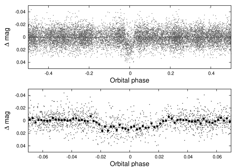
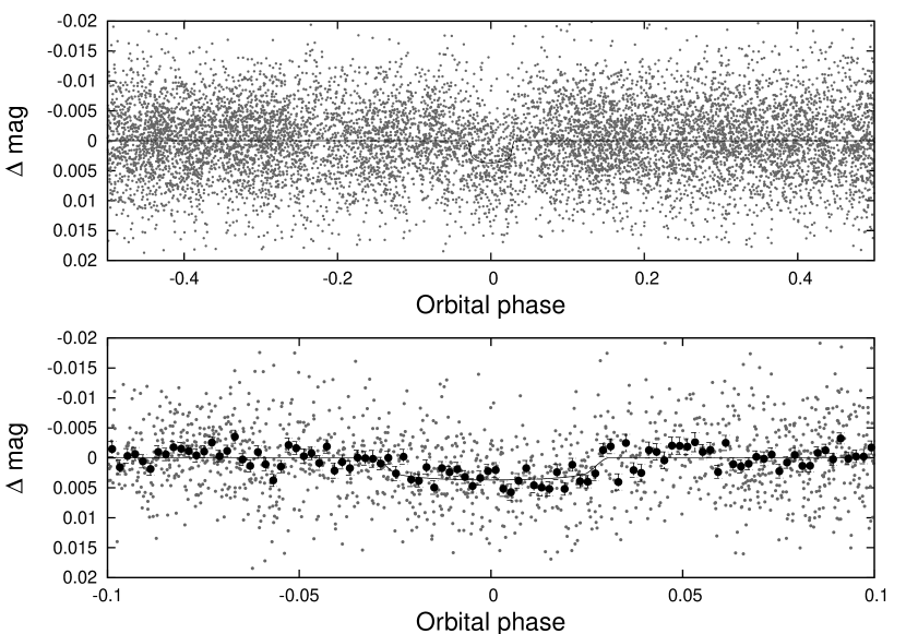
Figure 1.— Phase-folded unbinned HATSouth light curves for HATS-11 (left) and HATS-12 (right). In each case we show two panels. The top panel shows the full light curve, while the bottom panel shows the light curve zoomed-in on the transit. The solid lines show the model fits to the light curves. The dark filled circles in the bottom panels show the light curves binned in phase with a bin size of 0.002.

Table 1 Summary of photometric observations

Instrument/Field	Date(s)	# Images	Cadence	Filter	Precision
			(sec)		(mmag)
HATS-11
HS-3.1/G579	2010 Mar–2011 Aug	2229	304	$r$	11.5
HS-1.2/G579	2010 Mar–2011 Aug	4298	301	$r$	10.8
HS-3.2/G579	2010 Mar–2011 Aug	2144	304	$r$	11.2
HS-5.2/G579	2010 Sep–2011 Aug	2768	303	$r$	10.2
PEST	2013 Jun 15	138	131	$R_{C}$	4.9
Swope 1 m	2014 Jul 03	69	189	$i$	1.6
LCOGT 1 m+SBIG	2014 Sep 03	48	196	$i$	3.8
AAT+IRIS2	2014 Sep 07	778	16	$K_{S}$	3.7
LCOGT 1 m+Sinistro	2014 Sep 11	46	288	$i$	2.7
HATS-12
HS-1.2/G579	2010 Mar–2011 Aug	4315	300	$r$	5.9
HS-3.2/G579	2010 Mar–2011 Aug	2126	303	$r$	6.9
HS-5.2/G579	2010 Sep–2011 Aug	2781	303	$r$	6.1
PEST	2013 May 24	193	130	$R_{C}$	3.4
MPG 2.2m+GROND	2013 Jul 13	279	90	$g$	0.8
MPG 2.2m+GROND	2013 Jul 13	271	90	$r$	1.9
MPG 2.2m+GROND	2013 Jul 13	273	90	$i$	0.7
DK 1.54m+DFOSC	2013 Oct 03	98	145	$R$	1.9
SWOPE 1m	2015 May 26	82	59	$g$	2.1

2.2. Spectroscopic Observations

We started observing both candidates spectroscopically, in a process which is split into two kinds of spectroscopic observations. A first step of reconnaissance spectroscopy serves to reject possible astrophysical false positives, like e.g. binary stars, and to obtain a first estimate of stellar parameters. Afterwards, stable and high precision spectroscopic measurements allow us to obtain high precision radial velocity (RV) and line bisector (BS) time series for the stars. From this we can estimate the orbital parameters as well as the presence and mass of the companion for systems that are confirmed as planets, and a precise set of stellar parameters. The spectroscopic observations are summarized in Table 2.

HATS-11 was observed first with the ANU 2.3m telescope using the WiFES spectrograph and the duPont 2.5 m telescope using the echelle spectrograph. Details on the observing strategy and data reduction for the ANU 2.3m can be found in Bayliss et al. (2013) and for the duPont in Brahm et al. (2015). From these spectra we detect no RV variations greater than $\sim$2 $\rm km\,s^{-1}$  and could determine the host star’s spectral type. We verified with the new information that the transit is still consistent with a planetary companion. In light of this, we continued to observe HATS-11 with spectrographs allowing for simultaneous wavelength calibration for RV precision, namely with CORALIE at the Euler 1.2m and FEROS at the MPG 2.2m telescope. For both spectrographs we made use of the reduction procedures described in Jordán et al. (2014) which gave us the RV and BS measurements of the spectrum. Similarly, HATS-12 was observed with the WiFES and the duPont echelle spectrograph. RVs/BSs were obtained with FEROS and additionally with the HDS spectrograph at the Subaru telescope. Details on the data reduction with HDS can be found in Sato et al. (2002, 2012). The phased high-precision RV and BS measurements are shown for each system in Figure 2; the data are presented in Table 6. Spectra, RVs and BSs are used in Section 3 to reject some possible systems mimicking a planetary system.

Table 2 Summary of spectroscopy observations

Instrument	UT Date(s)	# Spec.	Res.	S/N Range	$\gamma_{\rm RV}$	RV Precision
			$\Delta\lambda$/$\lambda$/1000		($\rm km\,s^{-1}$)	($\rm m\,s^{-1}$)
HATS-11
ANU 2.3 m/WiFeS	2012 Sep 9	1	3	152	$\cdots$	$\cdots$
ANU 2.3 m/WiFeS	2012 Sep–2013 Mar	4	7	19–70	-53.8	4000
du Pont 2.5 m/Echelle	2013 Aug 21	1	40	40	-58.8	500
Euler 1.2 m/Coralie	2013 Aug–2014 Mar	10	60	11–17	-58.41	130
MPG 2.2 m/FEROS	2013 Apr–Sep	10	48	16–61	-58.32	42
HATS-12
MPG 2.2 m/FEROS	2012 Aug–2013 May	12	48	57–107	-21.66	42
ANU 2.3 m/WiFeS	2012 Sep 8	1	3	257	$\cdots$	$\cdots$
Subaru 8 m/HDS+I2	2012 Sep 19–22	9	60	53–86	$\cdots$	13
Subaru 8 m/HDS	2012 Sep 20	3	60	112-118	$\cdots$	$\cdots$
du Pont 2.5 m/Echelle	2013 Aug 21	1	40	58	-21.72	500

Figure 2.— Phased high-precision RV measurements for HATS-11 (left), and HATS-12 (right) from FEROS (open triangles), CORALIE (filled triangles), and HDS (filled circles). In each case we show three panels. The top panel shows the phased measurements together with our best-fit model (see Table 5) for each system. Solid lines show the best-fit circular orbit. Zero-phase corresponds to the time of mid-transit. The center-of-mass velocity has been subtracted. The second panel shows the velocity $O\!-\!C$ residuals from the best fit. The error bars include the jitter terms listed in Table 5 added in quadrature to the formal errors for each instrument. The third panel shows the bisector spans (BS), with the median value subtracted for each instrument. Note the different vertical scales of the panels.

2.3. Photometric follow-up observations

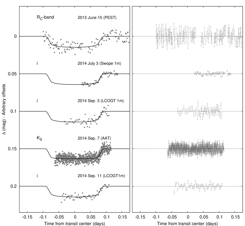
Figure 3.— Left: Unbinned transit light curves for HATS-11. The light curves have been corrected for quadratic trends in time fitted simultaneously with the transit model. The dates of the events, filters and instruments used are indicated. Light curves following the first are displaced vertically for clarity. Our best fit from the global modeling described in Section 3.3 is shown by the solid lines. Right: residuals from the fits are displayed in the same order as the left curves. The error bars represent the photon and background shot noise, plus the readout noise.

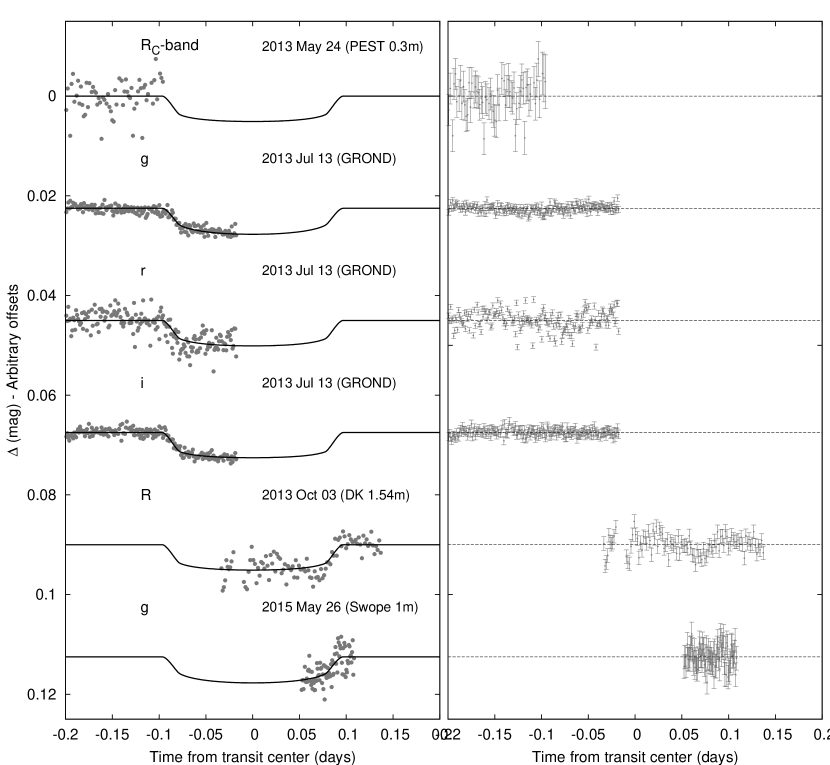
Figure 4.— Similar to Figure 3; here we show the follow-up light curves for HATS-12. The PEST 0.3 m, observation shows a flat out-of-transit  part. However, the observation helped to refine the ephemeris and the subsequent GROND observation detected the transit, see text.

We also photometrically followed-up both candidates with larger aperture telescopes. This is necessary because the HATSouth survey telescopes have limited photometric precision whereas the light curves  obtained with these follow-up telescopes are of higher quality allowing us to better characterize the system. The distant in time photometric follow-up observations further help us to refine the transit ephemeris. Photometric follow-up observations are summarized in Table 1. The data are given in Table 3. The light curves for HATS-11 are shown in Figure 3 while for HATS-12 they are shown in Figure 4.

We obtained photometric time series of HATS-11 with the PEST 0.3 m, Swope 1 m, and the LCOGT 1 m networks. Data reduction followed the established procedures described in previous HATSouth discoveries (Penev et al. (2013); Mohler-Fischer et al. (2013); Bayliss et al. (2013); Jordán et al. (2014); Zhou et al. (2014b); Hartman et al. (2015); Brahm et al. (2015); Mancini et al. (2015)).

Additionally, a partial transit of HATS-11b was observed on 2014-09-07, in the $K_{s}$-band, using the IRIS2 infrared camera (Tinney et al., 2004) on the 3.9 m Anglo Australian Telescope, at Siding Spring Observatory, Australia. The instrument uses a Hawaii 1-RG detector, has a field of view of $\rm 7.7\arcmin\times\rm 7.7\arcmin$, pixel scale of 0.4486$\rm\arcsec pixel^{-1}$. Exposures were 15 s in duration, with a total of 931 exposures taken, lasting a total of 4.6 hours. The target remained above airmass 1.25, and drifted by less than 1 pixel throughout the observations. The telescope was defocused to achieve a PSF FWHM of $\sim$2.2″, in order to minimize the effect of inter- and intra-pixel variation, and prevent saturation. The observing strategy, data reduction, and light curve analysis techniques are detailed in Zhou et al. (2014a). Flat fielding is performed using a linear combination of two sets of dither frames taken before and after the observation. Aperture photometry is performed on each frame to extract the fluxes of the target and reference stars. The target light curve  was corrected against the ensemble of reference stars, with weights to each reference star fitted for to minimize the out-of-transit  root mean square (RMS) scatter of the target star.

All observations of HATS-11b in different filters reproduced a similar flux decrease of $12.9$ mmag as seen in the discovery light curve, but with a higher precision, between 1.6 and 5 mmag per point. We note that mostly partial transits were observed. Each light curve allowed us to refine and improve the uncertainties of the ephemeris, which helped us to schedule subsequent transit observations. The final ephemeris is determined through the global MCMC analysis, as explained in Section 3.3, founding them to be $T_{c}({\rm BJD})=2456574.9657\pm 0.0013$ and $P=3.6191613\pm 0.0000099\,days$, as well as the parameters $R_{p}/R_{\star}=0.1076\pm 0.0028$ and $b^{2}=0.041_{-0.029}^{+0.060}$.

HATS-12 was observed with the PEST 0.3 m, MPG 2.2 m, DK 1.54 m and the Swope 1 m telescopes. Again, their light curves  were consistent with the discovery observations. For data analysis of the PEST, Swope and MPG2.2m observations we repeated our well established procedures as described in previous papers (Penev et al. (2013); Mohler-Fischer et al. (2013); Bayliss et al. (2013); Jordán et al. (2014); Zhou et al. (2014b); Hartman et al. (2015); Brahm et al. (2015); Mancini et al. (2015)). For the DK 1.54 m observation on the night 2013-10-03, we defocused the telescope. We used DFOSC, a focal reducer type camera with a $\rm 2048\times\rm 4096$ pixels E2V44-82 CCD. The CCD electronics was improved with a 32-bit analog-digital-converter (ADC), allowing for more levels than the usual 65536 available in 16-bit ADCs which are generally used for astronomical CCDs. The saturation obtained with this instrument is up to around 700000 $ADU$s with higher readout speed ($\rm 400\,kpix/s$) and higher gain of 0.24 $[e^{-}/ADU]$, and readout noise is 9.94 $e^{-}$. However, only half of the CCD is illuminated by the telescope  and this part of the CCD is readout and generally referred to as full frame, while further windowing is generally possible. The field-of-view (FOV) of the illuminated part is $\rm 13.7\arcmin\times\rm 13.7\arcmin$. This is sufficiently large to find adequate reference stars for our differential photometry. We choose a reference image and calculated the shift of all images with respect to the reference image. From the reference image we extracted the position of the stars. Following Deeg & Doyle (2013), the time series photometry was generated from these observations using optimized aperture photometry that maximizes the signal-to-noise ratio (SNR) for each star. For all images in one night we used three fixed apertures and choose these to be much larger than the typical point spread function in order to minimize the impact of the time-variable seeing. Depending on the telescope, for this bright object we obtained a follow-up precision between 0.7 and 3.4 mmag per point. The subsequent refinement of the transit ephemeris was especially important for HATS-12, as the first photometric follow-up observation with the PEST 0.3 m, telescope showed the flat out-of-transit  part. Despite that we did not detect the transit with the our initial ephemeris, this observation was still consistent with the transit having occurred after the observation, see upper most light curve in Figure 4. We updated the ephemeris so that the following photometric observation with GROND finally revealed the transit. Again, using the procedure described in Section 3.3, the final ephemeris was determined to be $T_{c}({\rm BJD})=2456798.9556\pm 0.0012$ and $P=3.142833\pm 0.000011\,days$, as well as the parameters $R_{p}/R_{\star}=0.0630\pm 0.0022$ and $b^{2}=0.347_{-0.132}^{+0.099}$.

Table 3 Light curve data for HATS-11 and HATS-12.

Object	BJD	Mag	$\sigma_{\rm Mag}$	Mag(orig)	Filter	Instrument
	(2,400,000$+$)
HATS-11	$55780.56087$	$-0.01727$	$0.00795$	$\cdots$	$r$	HS
HATS-11	$55762.46733$	$-0.01616$	$0.00787$	$\cdots$	$r$	HS
HATS-11	$55802.27850$	$0.01253$	$0.00731$	$\cdots$	$r$	HS
HATS-11	$55780.56478$	$0.01161$	$0.00824$	$\cdots$	$r$	HS
HATS-11	$55791.42313$	$-0.01754$	$0.01052$	$\cdots$	$r$	HS
HATS-11	$55762.47083$	$0.02251$	$0.00825$	$\cdots$	$r$	HS
HATS-11	$55802.28203$	$0.00687$	$0.00698$	$\cdots$	$r$	HS
HATS-11	$55273.88621$	$0.01511$	$0.00797$	$\cdots$	$r$	HS
HATS-11	$55791.42657$	$-0.01138$	$0.01137$	$\cdots$	$r$	HS
HATS-11	$55766.09292$	$0.00550$	$0.00705$	$\cdots$	$r$	HS

Note. — This table is available in a machine-readable form in the online journal. A portion is shown here for guidance regarding its form and content.

3. Analysis

3.1. Properties of the parent star

In order to obtain the physical parameters of the newly discovered planets, we have to characterize their stellar hosts. We determined precise atmospheric parameters for HATS-11 and HATS-12 from the median combined FEROS spectra. The SNR of both combined spectra was $\sim$50 per resolution element. We applied the algorithm ZASPE (Brahm et al. 2016, in prep) to both spectra which determines $T_{\rm eff}$, $\log{g}$, $\rm[Fe/H]$ and $v\sin{i}$ via least squares minimization against a grid of synthetic spectra in the most sensitive regions of the wavelength coverage to changes in the atmospheric parameters. ZASPE obtains reliable errors and correlations between the parameters that take into account the systematic mismatch between the data and the optimal synthetic spectra.

The $T_{\rm eff}$ and $\rm[Fe/H]$ values from ZASPE were combined with the stellar density ($\rho_{\star}$) which was obtained through our joint light curve and RV curve analysis to determine a first estimation of the stellar physical parameters (Sozzetti et al., 2007). In particular we search for the parameters of the Yonsei-Yale (Y2; Yi et al., 2001) isochrones (stellar mass, radius and age) that produce the best match with our estimated $T_{\rm eff}$, $\rm[Fe/H]$ and $\rho_{\star}$values. Then we compute a new value for $\log{g}$ which is held fix in a second run of ZASPE and a subsequent comparison with the theoretical isochrones is made. The final adopted parameters for HATS-11 and HATS-12 are given in Table 4. Figure 5 shows the locations of each star on a $T_{\rm eff\star}$–$\rho_{\star}$ diagram. We found after performing the analysis just described that both stars are slightly evolved metal poor stars. HATS-11 has a mass of 1.0$\pm$0.06 $M_{\sun}$, a radius of 1.444$\pm$0.057 $R_{\sun}$ and an age of 7.7$\pm$2 Gyr, while the parameters for HATS-12 are 1.489$\pm$0.071 $M_{\sun}$, 2.21$\pm$0.21 $R_{\sun}$ and an age of 2.36$\pm$0.3 Gyr. Distances are determined by comparing the measured broad-band photometry listed in Table 4 to the predicted magnitudes in each filter from the isochrones. We assume a $R_{V}=3.1$ extinction law from Cardelli et al. (1989) to determine the extinction.

Figure 5.— Model isochrones from Yi et al. (2001) for the measured metallicities of HATS-11 (left) and HATS-12 (right). For HATS-11 we show models for ages of 0.2 Gyr and 1.0 to 14.0 Gyr in 1.0 Gyr increments (ages increasing from left to right), while for HATS-12 we show models for ages of 0.2 Gyr, for 0.5 Gyr to 2.0 Gyr in 0.25 Gyr increments, and for 2.0 Gyr to 5.0 Gyr in 0.5 Gyr increments. The adopted values of $T_{\rm eff\star}$ and $\rho_{\star}$ are shown together with their 1$\sigma$ and 2$\sigma$ confidence ellipsoids. The initial values of $T_{\rm eff\star}$ and $\rho_{\star}$ from the first ZASPE and light curve analyses are represented with a triangle.

Table 4 Stellar parameters for HATS-11 and HATS-12

	HATS-11	HATS-12
Parameter	Value	Value	Source
Astrometric properties and cross-identifications
2MASS-ID	2MASS 19173618-2223236	2MASS 19164857-1921212
GSC-ID	GSC 6308-00430	GSC 6304-00396
R.A. (J2000)	$19^{\mathrm{h}}17^{\mathrm{m}}36.24{\mathrm{s}}$	$19^{\mathrm{h}}16^{\mathrm{m}}48.72{\mathrm{s}}$	2MASS
Dec. (J2000)	$-22{\arcdeg}23{\arcmin}23.7{\arcsec}$	$-19{\arcdeg}21{\arcmin}21.2{\arcsec}$	2MASS
$\mu_{\rm R.A.}$ ($\rm mas\,yr^{-1}$)	$4.5\pm 1.9$	$6.2\pm 4.0$	UCAC4
$\mu_{\rm Dec.}$ ($\rm mas\,yr^{-1}$)	$-21.5\pm 1.9$	$5.2\pm 2.7$	UCAC4
Galactic space velocity components, LSR reference frame
$u$ ($\rm km\,s^{-1}$)	65.274	25.812	FEROS+UCAC4
$v$ ($\rm km\,s^{-1}$)	88.956	37.784	FEROS+UCAC4
$w$ ($\rm km\,s^{-1}$)	40.364	-4.115	FEROS+UCAC4
Spectroscopic properties
$T_{\rm eff\star}$ (K)	$6060\pm 150$	$6408\pm 75$	ZASPE
$\rm[Fe/H]$	$-0.390\pm 0.060$	$-0.100\pm 0.040$	ZASPE
$v\sin{i}$ ($\rm km\,s^{-1}$)	$3.8\pm 1.0$	$6.57\pm 0.50$	ZASPE
$\gamma_{\rm RV}$ ($\rm km\,s^{-1}$)	$-58.324\pm 0.012$	$-21.661\pm 0.012$	FEROS
Photometric properties
$B$ (mag)	$14.657\pm 0.019$	$13.258\pm 0.043$	APASS
$V$ (mag)	$14.018\pm 0.081$	$12.756\pm 0.021$	APASS
$g$ (mag)	$14.268\pm 0.012$	$12.972\pm 0.005$	APASS
$r$ (mag)	$13.865\pm 0.039$	$12.654\pm 0.015$	APASS
$i$ (mag)	$13.506\pm 0.234$	$12.595\pm 0.021$	APASS
$J$ (mag)	$12.647\pm 0.023$	$11.725\pm 0.023$	2MASS
$H$ (mag)	$12.315\pm 0.025$	$11.507\pm 0.024$	2MASS
$K_{s}$ (mag)	$12.243\pm 0.025$	$11.391\pm 0.023$	2MASS
Derived properties
$M_{\star}$ ($M_{\sun}$)	$1.000\pm 0.060$	$1.489\pm 0.071$	YY+$\rho_{\star}$+ZASPE
$R_{\star}$ ($R_{\sun}$)	$1.444\pm 0.057$	$2.21\pm 0.21$	YY+$\rho_{\star}$+ZASPE
$\log{g_{\star}}$ (cgs)	$4.118\pm 0.026$	$3.923\pm 0.065$	YY+$\rho_{\star}$+ZASPE
$\rho_{\star}$ ($\rm g\,cm^{-3}$)	$0.471_{-0.052}^{+0.037}$	$0.196_{-0.044}^{+0.057}$	YY+$\rho_{\star}$+ZASPE
$L_{\star}$ ($L_{\sun}$)	$2.53\pm 0.39$	$7.3\pm 1.5$	YY+$\rho_{\star}$+ZASPE
$M_{V}$ (mag)	$3.81\pm 0.18$	$2.58\pm 0.22$	YY+$\rho_{\star}$+ZASPE
$M_{K}$ (mag,ESO)	$2.44\pm 0.10$	$1.47\pm 0.21$	YY+$\rho_{\star}$+ZASPE
Age (Gyr)	$7.7_{-1.6}^{+2.2}$	$2.36\pm 0.31$	YY+$\rho_{\star}$+ZASPE
$A_{V}$ (mag)	$0.42\pm 0.15$	$0.228\pm 0.068$	YY+$\rho_{\star}$+ZASPE
Distance (pc)	$906\pm 41$0	$981\pm 94$	YY+$\rho_{\star}$+ZASPE

3.2. Excluding blend scenarios

In order to exclude blend scenarios we carried out an analysis following Hartman et al. (2012). We attempt to model the available photometric data (including light curves and catalog broad-band photometric measurements) for each object as a blend between an eclipsing binary star system and a third star along the line of sight. The physical properties of the stars are constrained using the Padova isochrones (Girardi et al., 2000), while we also require that the brightest of the three stars in the blend have atmospheric parameters consistent with those measured with ZASPE.

For HATS-11 we find that the best-fit blend model provides a poorer fit to the data than the best-fit planet+star model, and can be rejected with $3\sigma$ confidence. Based on simulating composite spectra for the blend models that we tested, we also find that any blended eclipsing binary system that can plausibly fit the photometric data (i.e.  cannot be rejected with more than 5$\sigma$ confidence) would show BS variations ranging from $400$ $\rm m\,s^{-1}$ for the model that provides the most marginal fit (i.e.  at the 5$\sigma$ rejection limit), to more than $1$ $\rm km\,s^{-1}$ for the best-fitting blend models, as well as having RV variations with $K>200$ $\rm m\,s^{-1}$. As the measured BS variation is 80 $\rm m\,s^{-1}$ for FEROS and 140 $\rm m\,s^{-1}$ for Coralie, and the RV semiamplitude is $112\pm 15$ $\rm m\,s^{-1}$, we conclude that HATS-11 is not a blended stellar eclipsing binary system, and that the observations favor a transiting planet system interpretation. Similarly, for HATS-12 we find that the best-fit blend model provides a poorer fit to the data than the best-fit planet+star model, and in this case can be rejected with $2\sigma$ confidence. Those blended eclipsing binary systems that cannot be rejected with more than 5$\sigma$ confidence based solely on the photometry would have easily been detected as composite systems based on the FEROS and HDS spectroscopy, and would have BS variations exceeding 1 $\rm km\,s^{-1}$. For comparison, the BS RMS scatter is 34 $\rm m\,s^{-1}$ and 15 $\rm m\,s^{-1}$ for the FEROS and HDS observations of HATS-12, respectively. We conclude that HATS-12 is also not a blended stellar eclipsing binary system, and is instead a transiting planet system. However, both system could still be diluted transiting planet systems, which cannot be recognized by spectroscopic observations and only high angular resolution imaging can solve. If a blended stellar companion is present, diluting the light of the transiting system, then the true companion radius could be up to ∼60% larger than inferred.

3.3. Global modeling of the data

We modeled the HATSouth photometry, the follow-up photometry, and the high-precision RV measurements following Pál et al. (2008), Bakos et al. (2010) and Hartman et al. (2012). We fit Mandel & Agol (2002) transit models to the light curves, allowing for a dilution of the HATSouth transit depth as a result of blending from neighboring stars and over-correction by the trend-filtering method. For the follow-up light curves we include a quadratic trend in time in our model for each event to correct for remaining systematic errors in the photometry. We fit Keplerian orbits to the RV curves allowing the zero-point for each instrument to vary independently in the fit, and allowing for RV jitter which we also vary as a free parameter for each instrument. This jitter may be astrophysical or instrumental in nature, and simply represents excess scatter in the RV observations beyond what is expected based on formal uncertainties.

We used a Differential Evolution Markov Chain Monte Carlo procedure to explore the fitness landscape and to determine the posterior distribution of the parameters (DEMCMC; ter Braak, 2006). Note that we tried fitting both fixed circular orbits and free-eccentricity models to the data, and for both systems find that the data are consistent with a circular orbit. For both systems the fixed circular orbit model has a higher Bayesian evidence so we adopt the parameters obtained assuming no eccentricity for both objects. Furthermore, we see no structure or drift within our uncertainties that could hint to any extra component in the system. We also note that for HATS-11 the scatter in the CORALIE and FEROS RV residuals is consistent with the uncertainties, so our modeling finds jitter values of $0$ for both instruments. Similarly, we find that a jitter value of $0$ is preferred for the HDS observations of HATS-12. For these instruments we list the 95% upper limit on the jitter in the Table 5. The resulting parameters for each system are listed in Table 5. HATS-11b has a mass slightly smaller than Jupiter (0.85$\pm$0.12 $M_{\rm J}$) and a large radius of 1.51$\pm$0.078 $R_{\rm J}$. It is a moderately irradiated hot Jupiter with an equilibrium temperature of 1637$\pm$48 K. HATS-12b is a rather massive hot Jupiter with 2.38$\pm$0.11 $M_{\rm J}$, 1.35$\pm$0.17 $R_{\rm J}$  and a relatively high equilibrium temperature of 2097$\pm$ 89 K.

Table 5Orbital and planetary parameters for HATS-11b and HATS-12b

	HATS-11b	HATS-12b
Parameter	Value	Value
Light curve parameters
$P$ (days)	$3.6191613\pm 0.0000099$	$3.142833\pm 0.000011$
$T_{c}$ (${\rm BJD}$)	$2456574.9657\pm 0.0013$	$2456798.9556\pm 0.0012$
$T_{12}$ (days)	$0.1819\pm 0.0039$	$0.1899\pm 0.0031$
$T_{12}=T_{34}$ (days)	$0.0184\pm 0.0012$	$0.0167\pm 0.0033$
$a/R_{\star}$	$6.88_{-0.27}^{+0.18}$	$4.67\pm 0.38$
$\zeta/R_{\star}$	$12.23\pm 0.26$0	$11.54\pm 0.12$0
$R_{p}/R_{\star}$	$0.1076\pm 0.0028$	$0.0630\pm 0.0022$
$b^{2}$	$0.041_{-0.029}^{+0.060}$	$0.347_{-0.132}^{+0.099}$
$b\equiv a\cos i/R_{\star}$	$0.203_{-0.094}^{+0.115}$	$0.589_{-0.126}^{+0.079}$
$i$ (deg)	$88.31\pm 0.86$0	$82.7\pm 1.9$0
Limb-darkening coefficients
$c_{1},g$ (linear term)	$\cdots$	$0.4153$
$c_{2},g$ (quadratic term)	$\cdots$	$0.3276$
$c_{1},r$	$0.2778$	$0.2509$
$c_{2},r$	$0.3619$	$0.3789$
$c_{1},i$	$0.2115$	$0.1762$
$c_{2},i$	$0.3464$	$0.3706$
$c_{1},R$	$0.2590$	$0.2295$
$c_{2},R$	$0.3590$	$0.3783$
$c_{1},K$	$-0.0081$	$\cdots$
$c_{2},K$	$0.3305$	$\cdots$
RV parameters
$K$ ($\rm m\,s^{-1}$)	$112\pm 15$00	$250.6\pm 9.4$00
$e$	$<0.340$	$<0.085$
RV jitter FEROS ($\rm m\,s^{-1}$)	$<22.1$	$31\pm 16$
RV jitter Coralie ($\rm m\,s^{-1}$)	$<26.3$	$\cdots$
RV jitter HDS ($\rm m\,s^{-1}$)	$\cdots$	$<20.0$
Planetary parameters
$M_{p}$ ($M_{\rm J}$)	$0.85\pm 0.12$	$2.38\pm 0.11$
$R_{p}$ ($R_{\rm J}$)	$1.510\pm 0.078$	$1.35\pm 0.17$
$C(M_{p},R_{p})$	$0.15$	$0.57$
$\rho_{p}$ ($\rm g\,cm^{-3}$)	$0.299_{-0.050}^{+0.071}$	$1.19_{-0.32}^{+0.54}$
$\log g_{p}$ (cgs)	$2.959\pm 0.071$	$3.506\pm 0.095$
$a$ (AU)	$0.04614\pm 0.00093$	$0.04795\pm 0.00077$
$T_{\rm eq}$ (K)	$1637\pm 48$	$2097\pm 89$
$\Theta$	$0.0514\pm 0.0076$	$0.112_{-0.012}^{+0.018}$
$\log_{10}\langle F\rangle$ (cgs)	$9.211\pm 0.050$	$9.640\pm 0.074$

Note. — For both objects we list the parameters assuming circular orbits. Based on Bayesian evidence, we find that such an orbit is preferred for both systems.

4. Discussion

In this paper we have presented HATS-11b and HATS-12b, two inflated gas giants orbiting a metal-poor and a subsolar metallicity star with [Fe/H] of $-0.390\pm 0.060$ and $-0.100\pm 0.040$, respectively. Globally fitting all observations we estimated precise system parameters as shown in Tables 4-5.

HATS-11b and HATS-12b are two regular hot Jupiters that present inflated radii as compared to predictions of standard theoretical models of planetary structure. However, a distinction of these transiting systems is that both of them have low metallicity stellar hosts which are evolved.

Figure 6 shows a histogram of metallicity for known hot Jupiter planet hosts. The systems’ parameters were taken from the Transiting Extrasolar Planet Catalogue (TEPCat). We limited the sample to systems comparable to our discovered planets in this work by restricting it to TEPs satisfying $M_{P}\geq 0.47M_{J}$, $0.015\leq a\leq 0.5$ AU and around stars with 5300 K $\leq T_{\rm eff}\leq$ 7200 K (stellar spectral type G to F). The choice of 0.47 $M_{J}$ for the minimum mass is made based on the findings of Weiss et al. (2013) who found a break in the radius-mass relation at that mass. We also restrict the sample to have uncertainties in $\rm[Fe/H]$ $\leq$ 0.15 dex. As is now well established, giant planets are found less frequently around metal-poor stars. We note that HATS-11 is amongst the most metal poor stars detected to harbor a transiting giant planet and thus has the value of populating a sparse region of parameter space necessary to understand and validate planet formation theories. In particular, planets as massive as HATS-11b around stars with such a low metallicity can help to empirically constrain limits on the metallicity of the nebulae in the context of core-accretion theory, which can give insights of the boundaries of the formation process (Matsuo et al., 2007).

In Figure 7 we show stellar surface gravity as function of stellar radius for the same sample as in Figure 6. HATS-11 is a slightly evolved metal-poor star. Only two other systems resemble similar stellar parameters, namely HATS-9 (Brahm et al., 2015) and WASP-48 (Enoch et al., 2011), but none of them is metal-poor. Amongst the most evolved hot Jupiter hosts only two have a low metal content, namely HATS-12 and Kepler-435 (Almenara et al., 2015). No subsolar metallicity stars with similar stellar radius and surface gravity to HATS-12 have been detected so far, see Figure 7. Hence, HATS-11b and HATS-12b add new systems to the population of low-metallicity evolved stars known to host a giant planet.

Finally, we note that HATS-11 and HATS-12 were selected as targets for Kepler two-wheeled mission (K2) Campaign 7 (EPIC216414930 and EPIC218131080 respectively) under programs GO7066 and GO7067 (PI: Bakos). These targets have now been observed, and data is expected to be released on 2016 April 30. The high-precision K2 data will allow us to improve their transit parameters, especially important for HATS-12, as it shows the third shallowest ground-based transit discovery to date. Furthermore, we will have the possibility to search intensively for additional companions through the discovery of additional transits of longer period planets, see e.g. Rabus et al. (2009b), or transit timing variations (TTVs) (Rabus et al., 2009a), such as were measured in the hot Jupiter WASP-47b (Becker et al., 2015). The discovery of HATS-11b and HATS-12b thus provides a strong motivation for a combination of both ground-based detection and subsequent space-based follow-up characterization that can be fruitful and efficient.

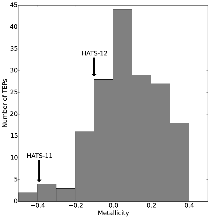
Figure 6.— Histogram of stellar metallicity for 177 hot Jupiter planet hosts, see text for population parameters. HATS-12 shows sub-solar metallicity, whereas HATS-11b transits a metal-poor star where fewer systems are well characterized.

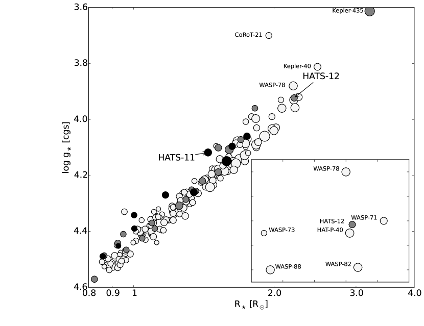
Figure 7.— Stellar surface gravity versus stellar radius of hot Jupiter planet hosts. The host stars’s metallicity is grey-color coded, grey circles show systems with $-0.2\leq$ $\rm[Fe/H]$$\leq-0.1$ dex and black circles $\rm[Fe/H]$$<-0.2$. The circle’s size reflect the planet’s radius. Both HATS-11 and HATS-12, occupy a region where only few planet hosts are known. The inset graph in the corner shows the region around HATS-12, with planet hosting stars of similar stellar radius, we note that HATS-12 is the only low metallicity system amongst the planet hosts with similar stellar parameters.

Table 6 Relative radial velocities and bisector spans for HATS-11 and HATS-12.

BJD	RV	$\sigma_{\rm RV}$	BS	$\sigma_{\rm BS}$	Phase	Instrument
(2,456,000$+$)	($\rm m\,s^{-1}$)	($\rm m\,s^{-1}$)	($\rm m\,s^{-1}$)	($\rm m\,s^{-1}$)
HATS-11
$400.76268$	$105.00$	$31.00$	$88.0$	$62.0$	$0.867$	FEROS
$411.71442$	$-23.00$	$47.00$	$21.0$	$94.0$	$0.893$	FEROS
$424.85662$	$-17.00$	$31.00$	$-56.0$	$62.0$	$0.524$	FEROS
$427.74603$	$-135.00$	$80.00$	$203.0$	$160.0$	$0.322$	FEROS
$488.81286$	$-55.00$	$31.00$	$-12.0$	$62.0$	$0.195$	FEROS
$490.79732$	$136.00$	$29.00$	$12.0$	$58.0$	$0.744$	FEROS
$492.73173$	$-100.00$	$28.00$	$-51.0$	$56.0$	$0.278$	FEROS
$524.50152$	$-103.59$	$80.00$	$213.0$	$160.0$	$0.057$	Coralie
$524.56679$	$34.41$	$69.00$	$106.0$	$138.0$	$0.075$	Coralie
$525.49132$	$-374.59$	$116.00$	$-76.0$	$232.0$	$0.330$	Coralie
$525.60831$	$40.41$	$128.00$	$-47.0$	$256.0$	$0.362$	Coralie
$544.52715$	$61.00$	$33.00$	$75.0$	$66.0$	$0.590$	FEROS
$548.59572$	$139.00$	$25.00$	$-27.0$	$50.0$	$0.714$	FEROS
$552.55423$	$105.00$	$30.00$	$-21.0$	$60.0$	$0.808$	FEROS
$727.88749$	$-126.59$	$75.00$	$-171.0$	$150.0$	$0.254$	Coralie
$728.85790$	$78.41$	$89.00$	$-30.0$	$178.0$	$0.522$	Coralie
$729.90376$	$114.41$	$88.00$	$-157.0$	$176.0$	$0.811$	Coralie
$730.90303$	$-105.59$	$144.00$	$30.0$	$288.0$	$0.087$	Coralie
$731.89440$	$40.41$	$141.00$	$51.0$	$282.0$	$0.361$	Coralie
$732.86378$	$246.41$	$143.00$	$247.0$	$286.0$	$0.629$	Coralie
HATS-12
$161.57017$	$-232.12$	$29.00$	$114.0$	$13.0$	$0.194$	FEROS
$161.58536$	$-320.12$	$28.00$	$44.0$	$13.0$	$0.199$	FEROS
$169.67026$	$238.88$	$26.00$	$35.0$	$12.0$	$0.772$	FEROS
$172.52620$	$224.88$	$24.00$	$-1.0$	$12.0$	$0.680$	FEROS
$189.80413$	$-221.85$	$12.01$	$-2.5$	$24.8$	$0.178$	HDS
$189.81885$	$-227.15$	$12.14$	$-2.7$	$23.2$	$0.183$	HDS
$189.83357$	$-191.54$	$11.86$	$-12.5$	$26.9$	$0.187$	HDS
$190.79653$	$\cdots$	$\cdots$	$1.4$	$22.5$	$0.494$	HDS
$190.81126$	$\cdots$	$\cdots$	$-9.7$	$18.7$	$0.498$	HDS
$190.82599$	$\cdots$	$\cdots$	$0.8$	$20.9$	$0.503$	HDS
$191.79963$	$233.55$	$15.50$	$8.3$	$25.0$	$0.813$	HDS
$191.81436$	$216.36$	$18.54$	$-1.9$	$31.0$	$0.818$	HDS
$191.82908$	$240.25$	$16.91$	$41.6$	$28.5$	$0.822$	HDS
$192.79563$	$-166.26$	$11.68$	$-16.2$	$19.2$	$0.130$	HDS
$192.81036$	$-182.37$	$14.01$	$-0.9$	$19.9$	$0.134$	HDS
$192.82509$	$-183.11$	$15.32$	$-5.6$	$26.0$	$0.139$	HDS
$211.59628$	$-220.12$	$22.00$	$22.0$	$11.0$	$0.112$	FEROS
$375.86732$	$-224.12$	$19.00$	$31.0$	$10.0$	$0.380$	FEROS
$376.87669$	$280.88$	$21.00$	$-12.0$	$11.0$	$0.701$	FEROS
$377.84700$	$-23.12$	$21.00$	$6.0$	$11.0$	$0.010$	FEROS
$398.86710$	$281.88$	$17.00$	$48.0$	$9.0$	$0.698$	FEROS
$402.87705$	$65.88$	$18.00$	$4.0$	$10.0$	$0.974$	FEROS
$405.87300$	$130.88$	$21.00$	$27.0$	$10.0$	$0.928$	FEROS
$426.93117$	$158.88$	$26.00$	$62.0$	$13.0$	$0.628$	FEROS

Note. — Note that for the HDS iodine-free template exposures we do not measure the RV but do measure the BS. Such template exposures can be distinguished by the missing RV value. The HDS observation of HATS-12 without a BS measurement has too low S/N in the I₂-free blue spectral region to pass our quality threshold for calculating accurate BS values.

References

- Almenara et al. (2015) Almenara, J. M., Damiani, C., Bouchy, F., et al. 2015, A&A, 575, A71
- Bakos et al. (2010) Bakos, G. Á., Torres, G., Pál, A., et al. 2010, ApJ, 710, 1724
- Bayliss et al. (2013) Bayliss, D., Zhou, G., Penev, K., et al. 2013, AJ, 146, 113
- Becker et al. (2015) Becker, J. C., Vanderburg, A., Adams, F. C., Rappaport, S. A., & Schwengeler, H. M. 2015, ApJ, 812, L18
- Brahm et al. (2015) Brahm, R., Jordán, A., Hartman, J. D., et al. 2015, AJ, 150, 33
- Buchhave et al. (2012) Buchhave, L. A., Latham, D. W., Johansen, A., et al. 2012, Nature, 486, 375
- Cardelli et al. (1989) Cardelli, J. A., Clayton, G. C., & Mathis, J. S. 1989, ApJ, 345, 245
- Claret (2004) Claret, A. 2004, A&A, 428, 1001
- Deeg & Doyle (2013) Deeg, H. J., & Doyle, L. R. 2013, VAPHOT: Precision differential aperture photometry package, Astrophysics Source Code Library
- Delrez et al. (2014) Delrez, L., Van Grootel, V., Anderson, D. R., et al. 2014, A&A, 563, A143
- Enoch et al. (2011) Enoch, B., Anderson, D. R., Barros, S. C. C., et al. 2011, AJ, 142, 86
- Everett et al. (2013) Everett, M. E., Howell, S. B., Silva, D. R., & Szkody, P. 2013, ApJ, 771, 107
- Girardi et al. (2000) Girardi, L., Bressan, A., Bertelli, G., & Chiosi, C. 2000, A&AS, 141, 371
- Hansen & Barman (2007) Hansen, B. M. S., & Barman, T. 2007, ApJ, 671, 861
- Hartman et al. (2011) Hartman, J. D., Bakos, G. Á., Torres, G., et al. 2011, ApJ, 742, 59
- Hartman et al. (2012) Hartman, J. D., Bakos, G. Á., Béky, B., et al. 2012, AJ, 144, 139
- Hartman et al. (2015) Hartman, J. D., Bayliss, D., Brahm, R., et al. 2015, AJ, 149, 166
- Henden & Munari (2014) Henden, A., & Munari, U. 2014, Contributions of the Astronomical Observatory Skalnate Pleso, 43, 518
- Johnson et al. (2010) Johnson, J. A., Aller, K. M., Howard, A. W., & Crepp, J. R. 2010, PASP, 122, 905
- Jordán et al. (2014) Jordán, A., Brahm, R., Bakos, G. Á., et al. 2014, AJ, 148, 29
- Kovács et al. (2005) Kovács, G., Bakos, G., & Noyes, R. W. 2005, MNRAS, 356, 557
- Kovács et al. (2002) Kovács, G., Zucker, S., & Mazeh, T. 2002, A&A, 391, 369
- Mancini et al. (2015) Mancini, L., Hartman, J. D., Penev, K., et al. 2015, A&A, 580, A63
- Mandel & Agol (2002) Mandel, K., & Agol, E. 2002, ApJ, 580, L171
- Matsuo et al. (2007) Matsuo, T., Shibai, H., Ootsubo, T., & Tamura, M. 2007, ApJ, 662, 1282
- Mohler-Fischer et al. (2013) Mohler-Fischer, M., Mancini, L., Hartman, J. D., et al. 2013, A&A, 558, A55
- Pál et al. (2008) Pál, A., Bakos, G. Á., Torres, G., et al. 2008, ApJ, 680, 1450
- Penev et al. (2013) Penev, K., Bakos, G. Á., Bayliss, D., et al. 2013, AJ, 145, 5
- Rabus et al. (2009a) Rabus, M., Deeg, H. J., Alonso, R., Belmonte, J. A., & Almenara, J. M. 2009a, A&A, 508, 1011
- Rabus et al. (2009b) Rabus, M., Alonso, R., Belmonte, J. A., et al. 2009b, A&A, 494, 391
- Santos et al. (2004) Santos, N. C., Israelian, G., & Mayor, M. 2004, A&A, 415, 1153
- Sato et al. (2002) Sato, B., Kambe, E., Takeda, Y., Izumiura, H., & Ando, H. 2002, PASJ, 54, 873
- Sato et al. (2012) Sato, B., Hartman, J. D., Bakos, G. Á., et al. 2012, PASJ, 64
- Schlaufman & Laughlin (2011) Schlaufman, K. C., & Laughlin, G. 2011, ApJ, 738, 177
- Sozzetti et al. (2007) Sozzetti, A., Torres, G., Charbonneau, D., et al. 2007, ApJ, 664, 1190
- ter Braak (2006) ter Braak, C. J. F. 2006, Statistics and Computing, 16, 239
- Tinney et al. (2004) Tinney, C. G., Ryder, S. D., Ellis, S. C., et al. 2004, in Society of Photo-Optical Instrumentation Engineers (SPIE) Conference Series, Vol. 5492, Ground-based Instrumentation for Astronomy, ed. A. F. M. Moorwood & M. Iye, 998–1009
- Valenti & Fischer (2005) Valenti, J. A., & Fischer, D. A. 2005, ApJS, 159, 141
- Wang & Fischer (2015) Wang, J., & Fischer, D. A. 2015, AJ, 149, 14
- Weiss et al. (2013) Weiss, L. M., Marcy, G. W., Rowe, J. F., et al. 2013, ApJ, 768, 14
- Yi et al. (2001) Yi, S., Demarque, P., Kim, Y.-C., et al. 2001, ApJS, 136, 417
- Zhou et al. (2014a) Zhou, G., Bayliss, D. D. R., Kedziora-Chudczer, L., et al. 2014a, MNRAS, 445, 2746
- Zhou et al. (2014b) Zhou, G., Bayliss, D., Penev, K., et al. 2014b, ArXiv e-prints, 1401.1582