Virial series for inhomogeneous fluids applied to the Lennard-Jones wall-fluid surface tension at planar and curved walls

Abstract

We formulate a straightforward scheme of statistical mechanics for inhomogeneous systems that includes the virial series in powers of the activity for the grand free energy and density distributions. There, cluster integrals formulated for inhomogeneous systems play a main role. We center on second order terms that were analyzed in the case of hard-wall confinement, focusing in planar, spherical and cylindrical walls. Further analysis was devoted to the Lennard-Jones system and its generalization the 2k-k potential. For this interaction potentials the second cluster integral was evaluated analytically. We obtained the fluid-substrate surface tension at second order for the planar, spherical and cylindrical confinement. Spherical and cylindrical cases were analyzed using a series expansion in the radius including higher order terms. We detected a $\ln R^{-1}/R^{2}$ dependence of the surface tension for the standard Lennard-Jones system confined by spherical and cylindrical walls, no matter if particles are inside or outside of the hard-walls. The analysis was extended to bending and Gaussian curvatures, where exact expressions were also obtained.

I Introduction

Equation of state (EOS) of a bulk fluid system contains the information about its thermodynamic behavior. For known potentials, virial expansion is a common method to calculate the EOS. This approach is usually limited to a certain low density region such as gas phase and must avoid transitions where the method is expected to break down. Additional problems comes from series convergence itself. Virial series are central for statistical mechanics (SM) theoretical development, hence they are a recurring topic even after 150 years.Waals (1873); Laar (1899); Ushcats (2013); Hellmann and Bich (2011); Shaul et al. (2012) There are several procedures that enable to obtain the EOS and other properties of the fluids by extrapolation of the first known terms of the virial series. Also, the first virial coefficients are used in the development of liquid theories, like density functionals or integral-differential equations.Gazzillo and Pini (2013); Beltran-Heredia and Santos (2014); Korden (2012)

Virial series are not only a major tool for simple and molecular fluids, but for colloidal systems. This systems are a mixture of two type of particles with a characteristic big size difference.Dudowicz et al. (2015); Koga et al. (2015); López de Haro et al. (2015) Nowadays, virial coefficients and cluster integrals are still under study, even at lower orders. There are several recent works about second order coefficients for diverse systems including inert gases, alkanes, methane in water solution, and polymer solutions.Hutem and Boonchui (2012); Schultz and Kofke (2010); Ashbaugh et al. (2015); Dudowicz et al. (2015); Koga et al. (2015) Distinct interaction models have been recently analyzed in this context: hard spheres with dipolar momentum,Virga (2013); Henderson (2011); Philipse and Kuipers (2010) exponential potential,Mamedov and Somuncu (2015) and the Asakura-Oosawa model for colloids.Santos et al. (2015); López de Haro et al. (2015); Koga et al. (2015); Dudowicz et al. (2015)

One of the most studied interaction models for simple fluids is the LJ. Modern studies based on molecular dynamics simulation shed light on its basic properties as viscosity, thermal conductivity, cavitation and melting coexistence.Baidakov et al. (2012); Baidakov and Protsenko (2014a, b); Baidakov and Bobrov (2014); Heyes and Brańka (2015) Other works have focused on the curvature dependence of the surface tension.Blokhuis and van Giessen (2013); Blokhuis and Kuipers (2007); van Giessen and Blokhuis (2002) The virial coefficients of the LJ fluid have been calculated numerically up to sixteenth order Gibbons and Steele (1971); Caligaris and Rodriguez (1971); Schultz and Kofke (2009a); Feng et al. (2015) and similar studies were done in LJ fluid mixtures up to sixth order.Schultz and Kofke (2009b) Second order coefficient is particularly relevant in this work. It was evaluated exactly for the first time in 2001 by Vargas et al.Vargas et al. (2001) and re-evaluated later.Eu (2009); Mamedov and Somuncu (2014) Generalizations to the so-called 2k-k LJ systemGlasser (2002) and extensions to non-conformal LJ model, were also done.González-Calderón and Rocha-Ichante (2015) We can mention that both, simple and colloidal fluids are continuously studied because some of their properties are yet not completely understood, being the 2k-k LJ interaction one of the models that enable to analyze them in a unified framework.

All the mentioned works about virial series refer to homogeneous fluids. In fact, most of the theoretical development about virial series is based on the original formulation and thus only apply to homogeneous systems.Mayer and Mayer (1940); Hill (1956); McQuarrie (2000); Hansen and McDonald (2006) Later generalizations adapted virial series expansions to inhomogeneous fluids and include external potentials. The seminal work on inhomogeneous systems was done by Bellemans in the sixties.Bellemans (1962a, b, 1963) Further developments were done by Sokolowski and Stecki,Sokołowski (1977); Sokołowski and Stecki (1979); Stecki and Sokołowski (1980) and by Rowlinson.Rowlinson (1986, 1985)

In this work we briefly introduce in a simple manner the statistical mechanics approach to inhomogeneous systems in grand canonical ensemble and its virial series. Our presentation focuses on a system of particles confined by the action of a general external potential following Rowlinson’s approach. We discuss virial series at the level of power series in the activity, where cluster integrands and integrals play a central role. To make simpler both notation and explanations the treatment is based on a one component system, and to some extent, to particles with pair-additive interaction. Despite this, extensions to mixtures including polyatomic molecules with internal degrees of freedom, and generalizations beyond the two-body potential that enable inclusion of multibody interactions are discussed. Alongside, our treatment of free energy, density distributions and other properties avoids the necessity of a volume definition. All the questions related to establish the volume and a reference bulk homogeneous system are also left to a separate analysis.

As an application we analyze the terms of second order for spherically symmetric pair interaction potentials. We solved for the first time the second order cluster integral for LJ and 2$k$-$k$ LJ fluids under inhomogeneous conditions. We evaluate analytically the cluster integral in non-trivial confinements: those produced by planar, spherical and cylindrical hard walls. Our expression is exact for the planar case. For curved walls we obtain several terms of the asymptotic expansion for large radii. To highlight the difficulty of the actual problem, we mention that up to date the only cluster integral analytically solved is that of second order and for the bulk case. This term corresponds to the pressure second virial coefficient.

Using the expression for the second cluster integral we study the properties of the LJ gas in contact with a curved hard wall, focusing on its surface tension. The question of how the properties of an inhomogeneous fluid depend on the curvature of its interface is a long standing problem in statistical mechanics.Blokhuis and van Giessen (2013) It has been thoroughly studied even for the interface induced by a curved substrate.Evans et al. (2003, 2004); Stewart and Evans (2005a, b); Blokhuis and Kuipers (2007); Reindl et al. (2015) We present rigorous results based on virial series about the curvature dependence of the properties of the LJ gas in contact with a curved wall which are exact up to power two in density.

The rest of this work is organized as follows: In Sec. II the SM of open systems with fixed chemical potential, temperature and external potential are revisited. Cluster integrals are thus shown in their inhomogeneous nature. Second order cluster terms are analyzed in Sec.III. There, the case of spherically interacting particles lying in a spatial region of arbitrary shape where they freely move is analyzed. We emphasize on three types of simple geometry confinements: planar, spherical and cylindrical walls. An application for the Lennard-Jones and the generalized 2$k$-$k$ Lennard-Jones systems is given in Sec.IV, where analytic expressions for the second cluster integral are derived. Sec. V is devoted to analyze the inhomogeneous low density gas, its wall-fluid surface tension, Tolman length and rigidity coefficients of bending and Gaussian curvatures. Finally, in Sec. VI we give our conclusions and final remarks.

II Theory

We consider an inhomogeneous system at a given temperature $T$, chemical potential $\mu$ (the number of particles may fluctuate) and external potential. The total potential energy also includes the contribution of mutual interaction between particles $\phi_{(n)}$. Thus, the grand canonical ensemble partition function (GCE) is

$$\Xi=1+\sum_{n=1}\lambda^{n}Q_{n}\>,$$ (1)

where $\lambda=\exp(\beta\mu)$ and $\beta=1/kT$ is the inverse temperature ($k$ is the Boltzmann’s constant). In Eq. (1) $Q_{n}$ is the canonical ensemble partition function

$$Q_{n} = \Lambda^{dn}Z_{n}/n!\>,$$ (2)

$$Z_{n} = \int g_{n}\left(\mathbf{x}\right)\exp\left(-\beta\phi_{(n)}\right)d\mathbf{x}\>,$$ (3)

where $\Lambda$ is the de Broglie thermal wavelength, $d$ is dimensionality and $Z_{n}$ is the configuration integral. $g_{n}\left(\mathbf{x}\right)=\prod_{i=1}^{n}g\left(\mathbf{x}_{i}\right)$, $g\left(\mathbf{x}_{i}\right)=\exp\left(-\beta\psi_{i}\right)$ and $\psi_{i}$ is the external potential over the particle $i$.

In Eq. (1) the sum index may end both at a given $m$ representing the maximum number of particles in the open system or at infinity. Fixing the value of $m$ allows the study of small systems.Rowlinson (1986) The main link between GCE and thermodynamics is still

$$\beta\Omega=-\ln\Xi\>.$$ (4)

Some thermodynamic magnitudes could be directly derived from $\Omega$ as $\left\langle n\right\rangle=-\beta\lambda\partial\Omega/\partial\lambda$. Yet, other thermodynamic magnitudes could be derived from $\Omega$ once volume and area measures of the system are introduced.

In the GCE several magnitudes can be expressed as power series in the activity $z=\lambda/\Lambda^{3}$ (virial series in $z$), with cluster integrals $\tau_{k}$ and cluster residual part as coefficients. The most frequent in the literature are

$$\beta\Omega = -\sum_{k=1}^{\infty}\frac{z^{k}}{k!}\tau_{k}\>,$$ (5)

$$\left\langle n\right\rangle = \sum_{k=1}^{\infty}\frac{kz^{k}}{k!}\tau_{k}\>,$$ (6)

$$\delta n = \left\langle n^{2}\right\rangle-\left\langle n\right\rangle^{2}=\sum_{k=1}^{\infty}\frac{k^{2}z^{k}}{k!}\tau_{k}\>.$$ (7)

Here $\left\langle n\right\rangle$ is the mean number of particles in the system and $\delta n$ measures the fluctuation of $\left\langle n\right\rangle$. Cluster integrals have played an important role in the development of virial expansion for homogeneous systems. For inhomogeneous fluids it is convenient to define the $n$-particles cluster integral $\tau_{n}$ as

$$\tau_{n}=n!\int g_{n}(\mathbf{x})\,b_{n}\left(\mathbf{x}_{1},\ldots,\mathbf{x}_{n}\right)d\mathbf{x}\>,$$

where $b_{n}\left(\mathbf{x}_{1},\ldots,\mathbf{x}_{n}\right)$ is the Mayer’s cluster integrand of order $n$. For simplicity, from here on we assume a pair potential interaction i.e. $\phi_{(n)}=\sum_{i,j}\phi_{ij}$, $\phi_{ij}=\phi\left(\mathbf{\mathbf{x}}_{ij}\right)$, being $\mathbf{\mathbf{x}}_{ij}=\mathbf{\mathbf{x}}_{j}-\mathbf{\mathbf{x}}_{i}$ the vector between $i$ and $j$ particles. Thus, $b_{n}\left(\mathbf{x}_{1},\ldots,\mathbf{x}_{n}\right)$ is the sum of all the product of Mayer’s function $f\bigl{(}\mathbf{\mathbf{x}}\bigr{)}=\exp\bigl{[}-\beta\phi\bigl{(}\mathbf{\mathbf{x}}\bigr{)}\bigr{]}-1$ that involves $n$ particles linked by $f$-bonds. In this sense $b_{n}\left(\mathbf{x}_{1},\ldots,\mathbf{x}_{n}\right)$ corresponds to clusters of $n$ particles.Yang et al. (2013) Note that $b_{1}=1$ and $\tau_{1}=Z_{1}$. For the density distributions the same approach is also useful. The one body density distribution isHill (1956); Hansen and McDonald (2006)

$$\rho\bigl{(}\mathbf{r}\bigr{)}=\bigl{\langle}\sum_{i=1}\delta\left(\mathbf{r}-\mathbf{x}_{i}\right)\bigr{\rangle}\>.$$

It is convenient to define the residual or $n$-cluster part of $\rho\bigl{(}\mathbf{r}\bigr{)}$, given by

$$\left\llbracket\rho^{(n)}\bigl{(}\mathbf{r}\bigr{)}\right\rrbracket=\frac{n}{Z_{n}}g_{1}\left(\mathbf{r}\right)\int g_{n-1}\left(\mathbf{x}\right)\,b_{n}\left(\mathbf{r},\mathbf{x}_{2},\ldots,\mathbf{x}_{n}\right)d\mathbf{x}\>,$$

which plays the role that cluster integrals do in Eq. (5). The virial series for $\rho\bigl{(}\mathbf{r}\bigr{)}$McQuarrie (2000) is

$$\rho(\mathbf{r}) = \sum_{k=1}^{\infty}\frac{z^{k}}{k!}Z_{k}\left\llbracket\rho^{(k)}(\mathbf{r})\right\rrbracket\>,$$ (8)

$$= \sum_{k=1}^{\infty}\frac{kz^{k}}{k!}\overline{\left\llbracket\rho^{(k)}(\mathbf{r})\right\rrbracket}\>.$$

Extension to other distribution functions are also direct. For example, for the two body distribution function one hasHansen and McDonald (2006)

$$\rho_{2}(\mathbf{r}_{1},\mathbf{r}_{2})=\bigl{\langle}\sum_{i=1}^{n}\sum_{j\neq i}^{n}\delta\left(\mathbf{r}_{1}-\mathbf{x}_{i}\right)\delta\left(\mathbf{r}_{2}-\mathbf{x}_{j}\right)\bigr{\rangle}\>,$$

$$\left\llbracket\rho_{2}^{(n)}(\mathbf{r}_{1},\mathbf{r}_{2})\right\rrbracket=\frac{n(n-1)}{Z_{n}}g_{1}(\mathbf{r}_{1})g_{1}(\mathbf{r}_{2})\exp\left[-\beta\phi(\mathbf{r}_{12})\right]\\ \times\int g_{n-2}(\mathbf{x})\,b_{n}\left(\mathbf{r}_{1},\mathbf{r}_{2},\mathbf{x}_{3},\ldots,\mathbf{x}_{n}\right)d\mathbf{x}\>,$$

$$\rho_{2}(\mathbf{r}_{1},\mathbf{r}_{2})=\sum_{k=2}^{\infty}\frac{z^{k}}{k!}Z_{k}\left\llbracket\rho_{2}^{(k)}(\mathbf{r}_{1},\mathbf{r}_{2})\right\rrbracket\>.$$

Treating particles 1 and 2 as linked, then $b_{n}\left(\mathbf{r}_{1},\mathbf{r}_{2},\mathbf{x}_{3},\ldots,\mathbf{x}_{n}\right)$ is the sum of all the cluster contributions of $n$ particles.McQuarrie (2000).

For homogeneous systems $g(\mathbf{x})=1$ and therefore $b_{n}(\mathbf{x})$ does not depend on the position, it reduces to the usual Mayer cluster coefficient $b_{n}$. Thus performing an extra integration

$$\tau_{n}=n!\int_{\infty}b_{n}(\mathbf{r})d\mathbf{r}=n!Vb_{n}\>,$$ (9)

with $V$ the volume of the accessible region, i.e., the infinite space or the cell when periodic boundary conditions are used.Hill (1956)

We have restricted our cluster decomposition to the case of two body interaction potentials. However, in Ref. Hellmann and Bich (2011) a systematic analysis of many body terms was done for virial expansions in homogeneous systems. It seems that with some minimal changes this approach is applicable to the inhomogeneous case. On the other hand, second order terms discussed in the next Sec. III are not modified when many-body interaction between particles are contemplated.

III Second order terms

The first non-trivial cluster terms are the ones of second order. They describe the physical behavior of the inhomogeneous low density gases up to order two in $z$. Our study of order terms use and generalize ideas and analytic procedures taken from Refs. Bellemans (1962a); Stecki and Sokołowski (1980). Thus, we turn to one body density distribution, its second order residual term is

$$\overline{\left\llbracket\rho^{(2)}(\mathbf{r}_{1})\right\rrbracket}\equiv g\bigl{(}\mathbf{r}_{1}\bigr{)}\int g\bigl{(}\mathbf{r}_{2}\bigr{)}f\bigl{(}\mathbf{r}_{12}\bigr{)}d\mathbf{r}_{2}\>.$$ (10)

Obtaining $\rho(\mathbf{r})$ up to order $z^{2}$ is reduced to solving this integral. In what follows, to proceed in the evaluation of order two cluster integrals, we gradually introduce some conditions on the system. We consider a system of spherical particles that interact through an spherically symmetric pair potential, and then, the Mayer function only depends on the distance between particles $r=\bigl{|}\mathbf{r}_{2}-\mathbf{r}_{1}\bigr{|}$. We focus on the important case where $g(\mathbf{r})=1$ if $\mathbf{r}\in\mathcal{A}$, a region bounded by the surface $\partial\mathcal{A}$, and is zero otherwise. Therefore $Z_{1}$ coincides with $V$, the volume of $\mathcal{A}$. The integrand of Eq. (10) can be written as $f(r)+[g(\mathbf{r}_{2})-1]\,f(r)$ and

$$\int\!g\bigl{(}\mathbf{r}_{2}\bigr{)}f\bigl{(}r\bigr{)}d\mathbf{r}_{2} = 2b_{2}-\!\int\!\left[1-g\bigl{(}\mathbf{r}_{2}\bigr{)}\right]f\bigl{(}r\bigr{)}d\mathbf{r}_{2}\>.$$ (11)

Here $1-g(\mathbf{r})=1$ if $\mathbf{r}\in\bar{\mathcal{A}}$ (where we introduce the complement of a set $\bar{\mathcal{A}}=\mathcal{A}\setminus\mathbb{R}^{3}$) and is zero otherwise. It is interesting to note that while the left hand side in Eq. (11) is $\int_{\mathcal{A}}f(r)d\mathbf{r}_{2}$ the integral on the right is $\int_{\bar{\mathcal{A}}}f(r)d\mathbf{r}_{2}$. Turning to Eq. (10) we note that the term $g(\mathbf{r}_{1})\int_{\bar{\mathcal{A}}}f(r)d\mathbf{r}_{2}$ is non-null only if $\mathbf{r}_{1}$ is in the neighborhood of $\partial\mathcal{A}$ because $\mathbf{r}_{1}\in\mathcal{A}$, $\mathbf{r}_{2}\in\bar{\mathcal{A}}$, and $r$ should be small enough to obtain $f(r)\neq 0$. Thus, this integral scales with the area of $\partial\mathcal{A}$. Now we restrict further analysis to cases where surface $\partial\mathcal{A}$ has constant curvature. We change integration variable $\mathbf{r}_{2}$ to relative coordinate between particles and introduce $u$ as the distance between $\mathbf{r}_{1}$ and $\partial\mathcal{A}$. For $\mathbf{r}_{1}\in\mathcal{A}$ we obtain

$$2\Delta b_{2}\equiv-\int_{\bar{\mathcal{A}}}f(r)d\mathbf{r}_{2}=-\int_{\bar{\mathcal{A}}}S(r,u)f(r)dr\>.$$ (12)

Here, $S(r,u)$ is the surface area of an spherical shell with radius $r$ and center $\mathbf{r}_{1}\in\mathcal{A}$ (at distance $u$ from $\partial\mathcal{A}$) that lies outside of $\mathcal{A}$. In Fig. 1 we give some insight about geometry-related magnitudes for some simple shapes of $\partial\mathcal{A}$. The final result is thus

$$\left\llbracket\rho^{(2)}(\mathbf{r}_{1})\right\rrbracket=\frac{2}{Z_{2}}g\bigl{(}\mathbf{r}_{1}\bigr{)}\left[2b_{2}+2\Delta b_{2}(u)\right]\>,$$ (13)

$$2\Delta b_{2}(u)=-\int_{r_{min}(u)}^{r_{max}(u)}S(r,u)f(r)dr\>,$$ (14)

where the boundary of the integration domain is explicit.

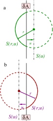
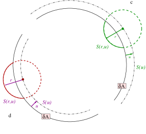
Figure 1: Integration schemes for $\Delta b_{2}(\mathbf{r})$ and $\Delta\tau_{2}$. Planar case corresponds to both (a) and (b). Spherical and cylindrical cases correspond to (c) and (d). Diagram (c) is for fluids outside of the region enclosed by the curved surface, while diagram (d) is for fluids inside this region. Note that (c) and (d) in the limit $R\rightarrow\infty$ corresponds to (a) and (b), respectively, which are equivalent.

Now we consider $\tau_{2}$, given by

$$\tau_{2}\equiv\iint g(\mathbf{r}_{1})g(\mathbf{r}_{2})f\bigl{(}\mathbf{r}_{12}\bigr{)}d\mathbf{r}_{1}d\mathbf{r}_{2}\>.$$ (15)

and follow an approach similar to that used to transform Eq. (10). For spherically symmetric pair potentials and a region $\mathcal{A}$ with arbitrary shape we found

$$\tau_{2} = 2Z_{1}b_{2}+\Delta\tau_{2}\>,$$

$$\Delta\tau_{2} = -\int_{\mathcal{A}}\left[\int_{\bar{\mathcal{A}}}f\bigl{(}r\bigr{)}d\mathbf{r}_{2}\right]d\mathbf{r}_{1}\>.$$ (16)

Remarkably, $\Delta\tau_{2}$ is invariant under the interchange $\bar{\mathcal{A}}\leftrightarrow\mathcal{A}$ no matter the details of the potential between particles. It implies that the inhomogeneous contribution to $\tau_{2}$ is the same if the system is confined in a box or if it is confined to all the space outside the box, ignoring of the shape of the box. This in-out symmetry has been previously studied.Urrutia (2008, 2010) It has a second interesting physical implication: if giving a certain shape of $\mathcal{A}$ some terms of $\Delta\tau_{2}$ should change its sign under the interchange $\bar{\mathcal{A}}\leftrightarrow\mathcal{A}$ all of them must be identically zero. For the case of a surface $\partial\mathcal{A}$ with constant curvature we transform integration variables $\mathbf{r}_{1}$ and $\mathbf{r}_{2}$, to position with respect to $\partial\mathcal{A}$ and relative coordinate between particles. Once the trivial integrations are done one finds

$$\Delta\tau_{2}=-\int_{\mathcal{A}}S(u)\left[\int_{\bar{\mathcal{A}}}S(r,u)f\bigl{(}r\bigr{)}dr\right]du\>.$$ (17)

Here, $S(u)$ is the area of the surface parallel to $\partial\mathcal{A}$ at a distance $u$ that lies in $\mathcal{A}$. Fig. 1 shows a picture of the overall approach for some simple shapes of $\partial\mathcal{A}$. Expressions for $S(r,u)$ are known for planar, spherical and cylindrical shapes of $\partial\mathcal{A}$ which shows that Eq. (17) is an interesting formula to analytically evaluate $\tau_{2}$. Finally, one can introduce the boundary of the integration domain to obtain the following two equivalent expressions

$$\Delta\tau_{2}=-\int_{u_{min}}^{u_{max}}S(u)\left[\int_{r_{min}(u)}^{r_{max}(u)}S(r,u)f(r)dr\right]du\>$$ (18)

[where the term in brackets is $2\Delta b_{2}(u)$] and

$$\Delta\tau_{2}=-\int_{r_{min}}^{r_{max}}f(r)\left[\int_{u_{min}(r)}^{u_{max}(r)}S(u)S(r,u)du\right]dr\>.$$ (19)

Both expressions enable to evaluate $\Delta\tau_{2}$ for very simple potentials like that of HS. Even though, Eq. (19) condensates the geometrical constraint in the inner integral over $u$ while the nature of the interaction remains in $f(r)$. Thus, Eq. (19) is a convenient starting point to analyze a variety of not so simple pair potentials. Next paragraphs introduce further simplifications on Eqs. (14) and (19) for planar, spherical and cylindrical confinements.

For planar walls

In the planar case $S(r,u)=2\pi r(r-u)$, $r(u)_{min}=u$, $r_{max}(u)=\infty$ and Eq. (14) takes the form

$$2\Delta b_{2}(u)=-2\pi\int_{u}^{\infty}(r^{2}-u\,r)f(r)dr\>.$$ (20)

Obviously, $S(u)=A$, which corresponds to the area of an infinite plane or the finite area of the hard plane in the unit cell when periodic boundary conditions are used. Although, $r_{min}=0$, $r_{max}=\infty$, $u_{min}(r)=0$ and $u_{max}(r)=r$. Therefore, Eq. (19) reduces to

$$\Delta\tau_{2}=-2Aa_{2}\textrm{, with }a_{2}=\frac{\pi}{2}\int_{0}^{\infty}f(r)r^{3}dr\>.$$ (21)

It is interesting to compare Eq. (21) with the bulk second cluster integral of a system in a region of volume $V$,

$$\tau_{2}=2Vb_{2}\textrm{, with }b_{2}=2\pi\int_{0}^{\infty}f(r)r^{2}dr\>,$$ (22)

that gives the bulk system second virial coefficient $B_{2}=-b_{2}$. Thus we show that the difficult of solving the terms $2\Delta b_{2}(u)$ and $\Delta\tau_{2}$ for an inhomogeneous fluid confined by a planar wall is similar to the one of solving the bulk fluid term $\tau_{2}$. Both $\Delta b_{2}$ and $\Delta\tau_{2}$ are known for the HS and the SW systems.Bellemans (1962b); Stecki and Sokołowski (1980)

For spherical walls

Again, we start from Eq. (19). Two different situations arise because the system may be inside the sphere with area $A=4\pi R^{2}$ and volume $V=4\pi R^{3}/3$ or outside of it. If the fluid is outside of the spherical surface $\partial\mathcal{A}$ then $u:(0,\infty)$, $S(u)=4\pi(R+u)^{2}$ and $S(r,u)=\pi r(r-u)(2R+u-r)/(R+u)$. On the opposite, for fluids inside the spherical shell $\partial\mathcal{A}$ one finds $u:(0,R)$, $S(u)=4\pi(R-u)^{2}$ and, if $u<r<2R-u$ then $S(r,u)=\pi r(r-u)(2R-u+r)/(R-u)$ but if $r>2R-u$ then $S(r,u)=4\pi r^{2}$. For a geometrical insight see Fig. 1 (c) and (d).

In the case of a fluid that surrounds an spherical object we have

$$2\Delta b_{2}(u)=\frac{\pi}{R+u}\int_{u}^{2R+u}\!\!\!\!f(r)r(u-r)(2R+u-r)dr\>,$$ (23)

and if the fluid is inside of an spherical cavity we have:

$$2\Delta b_{2}(u) = \frac{\pi}{R-u}\int_{u}^{2R-u}\!\!\!\!f(r)r(u-r)(2R-u+r)dr-$$ (24)

$$4\pi\int_{2R-u}^{\infty}f(r)r^{2}dr\>.$$

To evaluate $\Delta\tau_{2}$ one may assume that the fluid is outside of an spherical shell to obtain

$$\Delta\tau_{2}=-\int_{0}^{\infty}f(r)w(r)dr\>,$$ (25)

with $w(r)=A\pi r^{3}-\frac{1}{3}\pi^{2}r^{5}$ for $0<r\leq 2R$ while $w(r)=V4\pi r^{2}$ for $r>2R$. We have verified that Eq. (25) [with the same expression for $w(r)$] also applies to the case of fluid inside of a spherical shell. The situation of small curvature is simpler to analyze by writing

$$\Delta\tau_{2}=-2Aa_{2}+2c_{2}+2d_{2}\>,$$ (26)

where $a_{2}$ was defined in Eq. (21) and

$$c_{2} = \frac{\pi^{2}}{6}\int_{0}^{\infty}f(r)r^{5}dr\>,$$ (27)

$$d_{2} = \int_{2R}^{\infty}f(r)\left(-V2\pi r^{2}+A\frac{\pi}{2}r^{3}-\frac{\pi^{2}}{6}r^{5}\right)dr\>,$$ (28)

those make sense if $c_{2}$ converges. Note that $a_{2}$ and $c_{2}$ depend on temperature but not on $R$. Although, $d_{2}$ in Eq. (26) may include terms $\mathcal{O}(R^{0})$ and higher order ones in $R^{-1}$. If $c_{2}$ does not converge, it is preferable to define a single term $\tilde{c}_{2}=c_{2}+d_{2}$ as

$$\tilde{c}_{2}=\frac{\pi^{2}}{6}\!\!\int_{0}^{2R}\!\!\!f(r)r^{5}dr-\!\int_{2R}^{\infty}\!\!f(r)(V2\pi r^{2}-A\frac{\pi}{2}r^{3})dr\,.$$ (29)

Note that Eqs. (26-29) apply to both, finite values of $R$ and the case of small curvature $R\gg 1$.

Interestingly, if the pair potential is of finite range smaller than $2R$, integral $c_{2}$ converges, $d_{2}=0$, $a_{2}$ and $c_{2}$ are functions of $T$ (do not depend on $R$), and

$$\Delta\tau_{2}=-2Aa_{2}+2c_{2}\>,$$ (30)

without the term of order $R$. For example, this is the case of the truncated 12-6 Lennard Jones potential (it does not matter if it is shifted or not) which is frequently used in simulations and theoretical development.Allen and Tildesley (1987); Shaul et al. (2010) Naturally, it is also the case of the hard sphere (HS) and square well (SW) interactions. For HS and SW fluids one finds

$$b_{2}=-\frac{2\pi}{3}\>,\>\>a_{2}=-\frac{\pi}{8}\>,\>\>c_{2}=-\frac{\pi^{2}}{36}\>,$$ (31)

$$b_{2}=\frac{-2\pi}{3}\Sigma(3)\,,\>a_{2}=-\frac{\pi}{8}\Sigma(4)\,,\>c_{2}=-\frac{\pi^{2}}{36}\Sigma(6)\>,$$ (32)

respectively (here results are given in units of the hard-core diameter $\sigma$, $\Sigma(x)=\lambda^{x}+e^{-\beta\epsilon}(1-\lambda^{x})$, being $\lambda$ the range of the square well and $\epsilon$ its depth). These results are consistent with those found previously using different approachesBellemans (1963); McQuarrie and Rowlinson (1987); Urrutia (2010); Urrutia and Castelletti (2011) and serve here to cross-check new expressions.

For cylindrical walls

In this geometry the system may be inside the cylinder of area $A=2\pi R\,L$ and volume $V=\pi R^{2}L$ or outside of it. Now, if the fluid is outside of the cylindrical surface $\partial\mathcal{A}$ then, $S(u)=2\pi\left(R+u\right)L$, else, if it is inside the cylindrical wall then $S(u)=2\pi\left(R-u\right)L$. Note that in this case $L$ is the length of an infinite cylinder or a finite length when periodic boundary conditions are used. Analytic expression of $S(r,u)$ involves elliptic integrals of the first, second and third kindLamarche and Leroy (1990) and are given in the Appendix A. To evaluate $\Delta\tau_{2}$ one may assume again that the fluid is outside of the cylindrical shell and obtain a relation identical to Eq. (25). However, for the cylindrical confinement we do not find a simple analytic expression for $w$. For large $R$ the series expansion of $S(r,u)$ provides the expression

$$w(r)=A\pi r^{3}-L\left(\frac{\pi^{2}r^{5}}{16R}+\frac{\pi^{2}r^{7}}{512R^{3}}\right)+\mathcal{O}(r^{9}R^{-5})\>,$$ (33)

which applies to the region $0<r<2R$.

Thus, we obtain

$$\Delta\tau_{2}=-2Aa_{2}+2x_{2}+2d_{2}\>,$$ (34)

$$x_{2}=\frac{L}{R}\frac{3}{16}c_{2}\>,$$ (35)

[$a_{2}$ and $c_{2}$ are given by Eqs. (21, 27)] and

$$d_{2} = \int_{2R}^{\infty}f(r)\left(-V2\pi r^{2}+A\frac{\pi}{2}r^{3}-\frac{L}{R}\frac{\pi^{2}}{32}r^{5}\right)dr+$$ (36)

$$L\int_{0}^{2R}f(r)\left[\frac{\pi^{2}r^{7}}{1024R^{3}}+\mathcal{O}\left(\frac{r^{9}}{R^{5}}\right)\right]dr\>.$$

Naturally this makes sense if $x_{2}$ (i.e. $c_{2}$) converges. Otherwise, it is convenient to define a single term $\tilde{x}_{2}=x_{2}+d_{2}$ following the same criteria adopted in Eq. (29). When the pair potential has finite range smaller than $2R$ the convergence of $c_{2}$ is secured, first term of $d_{2}$ is null but higher order terms in $R^{-1}$ do not disappear in the cylindrical case. We found for the HS and SW particles,

$$x_{2}=-\frac{\pi^{2}}{192}\textrm{ and }x_{2}=-\frac{\pi^{2}}{192}\Sigma(6)\>.$$ (37)

The HS result was found before utilizing a different method but SW result is new.Urrutia (2010)

IV Case study: $\tau_{2}$ for the confined Lennard-Jones fluid

Virial series in general and specifically its truncation at second order coefficient $B_{2}$ have been thoroughly studied for a long time because they enable to analytically describe the properties of diluted homogeneous fluids. Beyond the case of HS and SW potentials, analytic expressions of $B_{2}(T)$ were found for the 12-6 Lennard-Jones (LJ) potentialVargas et al. (2001), for the $2k$-$k$ LJ potentialGlasser (2002) and others LJ-like potentials.González-Calderón and Rocha-Ichante (2015) For molecular dynamic simulation purposes the truncation of interaction potential at finite range is necessary. Yet, virial coefficients of truncated-LJ systems were numerically evaluated.Shaul et al. (2010)

Virial series are not a standard method to study inhomogeneous fluids. Nonetheless, a few recent works studied the inhomogeneous HS fluid under this framework.Yang et al. (2013); Urrutia (2014); Yang et al. (2015) In the case of inhomogeneous LJ fluid we found a single work that based on this series (truncated at second order) study the adsorption of 12-6 LJ gas on a planar attractive wall.Stecki and Sokołowski (1980) There, second order cluster integral is numerically evaluated. In the following, cluster integral $\tau_{2}$ for the inhomogeneous 2k-k LJ confined by hard walls of constant curvature is evaluated analytically for the first time.

IV.1 $\tau_{2}$ for the inhomogeneous Lennard-Jones fluid

Here we evaluate analytically $\tau_{2}$ by applying to Eqs. (20) and (21) some ideas and procedures partially taken from Refs. Vargas et al. (2001); Glasser (2002). We generalize those calculus to obtain the second cluster integral for planar spherical, and cylindrical confinement.

One can observe that several of the integrals appearing in Sec. III are of the form $\int_{a_{1}}^{a_{2}}f(r)r^{m}dr$. For $m=2$ (and $a_{1}=0$, $a_{2}\rightarrow\infty$) it corresponds to $b_{2}$ and $B_{2}$ that describe homogeneous systems [see Eq. (22)]. We introduce the $2k$-$k$ LJ pair potential

$$\phi(r)=4\epsilon\left[\left(\frac{\sigma}{r}\right)^{2k}-\left(\frac{\sigma}{r}\right)^{k}\right]\>,$$ (38)

with $k\geq 6$. The case $k=6$ is the most used to model simple monoatomic fluids, yet higher values like $k=18$ are utilized in studies of particles with short range interaction potential as neutral colloids.Vliegenthart and Lekkerkerker (2000) Thus, we shall solve integrals of the type

$$\int\sigma^{-(m+1)}\left\{\exp\left[-\beta\phi(r)\right]-1\right\}r^{m}dr\>.$$ (39)

with $0<m+1\leq k$. In the case of Eqs. (21, 22) and (27) the integration domain $(0,\infty)$ leave us with indefinite integrals. Changing variable to $x=r/\sigma$ and defining $z=4\beta\epsilon$ one finds

$$C_{m+1,k}=\int_{l_{1}}^{l_{2}}\left\{\exp\left[-z\left(x^{-2k}-x^{-k}\right)\right]-1\right\}x^{m}dx\>,$$ (40)

where $l_{2}$ is typically $\sigma/2R$ or $\infty$. Changing variables to $y=x^{k}$ it transforms to

$$C_{m+1,k}=\frac{1}{k}\int_{l_{1}^{k}}^{l_{2}^{k}}y^{q-1}\left\{\exp\left[-z\left(y^{-2}-y^{-1}\right)\right]-1\right\}dy\>.$$ (41)

where $q=\frac{m+1}{k}$. A comparison between Eqs. (40) and (41) shows that $C_{m+1,k}=\frac{1}{k}C_{q,1}$. We transform variables to $u=y^{-1}$ and fix $l_{1}^{-k}=M$ (i.e. $l_{1}=M^{-1/k}$) and $l_{2}^{-k}=\varepsilon$ to obtain

$$C_{q,1}=\int_{\varepsilon}^{M}u^{-(q+1)}\left\{\exp\left[-z\left(u^{2}-u\right)\right]-1\right\}du\>.$$ (42)

It is convenient to define $C_{q}(\varepsilon)=\underset{M\rightarrow\infty}{\lim}C_{q,1}$ to analyze the condition $l_{1}=0$ and thus we assume $q>0$ to prevent the divergence. Once we integrate Eq. (42) by parts we obtain

$$qC_{q}(\varepsilon)=\varepsilon^{-q}\!\left\{\exp\!\left[-z\!\left(\varepsilon^{2}-\varepsilon\right)\right]\!-\!1\right\}+I_{q,\varepsilon}-2I_{q-1,\varepsilon}$$ (43)

where $I_{\nu,\varepsilon}=z\int_{\varepsilon}^{\infty}u^{-\nu}\exp\left[-z\left(u^{2}-u\right)\right]du$. $I_{\nu}=I_{\nu,0}$ and $C_{q}(0)$ were studied by Glasser Glasser (2002) who gives closed expressions for $\nu<1$ and $0<q<1$, respectively, in terms of Kummer’s hypergeometric functions. In Appendix B we analyze the functions $I_{\nu,\varepsilon}$ and $C_{q}(\varepsilon)$, and provide explicit expressions of them when $0<\varepsilon\ll 1$.

Before analyzing the asymptotic behavior at large radius we give in terms of $C_{q}$ the following exact expressions

$$\frac{\tau_{2}}{2}=V\frac{2\pi}{k}C_{3/k}(0)-A\frac{\pi}{2k}C_{4/k}(0)\>,$$ (44)

$$\left.\frac{\tau_{2}}{2}\right|_{\textrm{in}}=V\frac{2\pi}{k}C_{3/k}(\varepsilon)-A\frac{\pi}{2k}C_{4/k}(\varepsilon)+\frac{\pi^{2}}{6k}C_{6/k}(\varepsilon)\>,$$ (45)

which apply to the planar and spherical cases, respectively. In Eq. (45) and from now on we fix $\varepsilon=\left(2R\right)^{-k}$ ($\sigma$ is the unit length). For the cylindrical case we found

$$\left.\frac{\tau_{2}}{2}\right|_{\textrm{in}} = V\frac{2\pi}{k}C_{3/k}(\varepsilon)-A\frac{\pi}{2k}C_{4/k}(\varepsilon)+$$ (46)

$$\frac{L}{R}\frac{\pi^{2}}{32k}C_{6/k}(\varepsilon)+\frac{L}{R^{3}}\frac{\pi^{2}}{512k}C_{8/k}(\varepsilon)+....\>,$$

where higher order $C_{q}$ functions were neglected. In the limit of large $R$ ($\varepsilon\rightarrow 0$) we found the following expressions for $B_{2}=-b_{2}$, $b_{2}$, $a_{2}$, $c_{2}$, $d_{2}$ and $\tilde{c}_{2}$:

$$b_{2} = \frac{2\pi}{k}C_{3/k}(0)\>,$$ (47)

$$a_{2} = \frac{\pi}{2k}C_{4/k}(0)\>,$$ (48)

$$c_{2} = \frac{\pi^{2}}{6k}C_{6/k}(0)\>,$$ (49)

that are given in $\sigma$ units. Explicit form of $C_{q}(0)$ in terms of hypergeometric functions is given in Appendix B Eq. (77). Note that Eq. (49) applies if $k>6$, when $c_{2}$ converges. In this case $d_{2}=-\frac{V2\pi}{k}\Delta C_{3/k}+\frac{A\pi}{2k}\Delta C_{4/k}-\frac{\pi^{2}}{6k}\Delta C_{6/k}$ with $\Delta C_{q}=C_{q}(0)-C_{q}(\varepsilon)$. From the series expansion we obtain

$$d_{2}=-(2R)^{6-k}\frac{4\pi^{2}}{T(k-6)(k-4)(k-3)}+\mathcal{O}(R^{6-2k})\>.$$ (50)

The relevant case $k=6$ corresponds to the 12-6 LJ potential which produces $\tilde{c}_{2}=-\frac{V\pi}{3}\Delta C_{1/2}+\frac{A\pi}{12}\Delta C_{2/3}+\frac{\pi^{2}}{36}C_{1}(\varepsilon)$. It can be split in

$$c_{2}=\frac{\pi^{2}}{18T}\left[12\ln\left(2R\right)+\ln\left(\frac{T}{4}\right)+10\right]+\frac{\pi^{2}}{36}reg[C_{1}(0)]\>,$$ (51)

$$d_{2}=(2R)^{-6}\frac{\pi^{2}(T-2)}{108T^{2}}+\mathcal{O}(R^{-12})\>,$$ (52)

where $reg[C_{1}(0)]$ is the regular (non-divergent) part of $C_{1}(\varepsilon)$ in the limit $\varepsilon\rightarrow 0$. For cylindrical walls the details of the calculus are given in the Appendix C. Here we show the main results: if $k>6$ then $x_{2}=\frac{L}{R}\frac{3}{16}\frac{\pi^{2}}{6k}C_{6/k}(0)$ [from Eqs. (35) and (49)] else, if $k=6$ then

$$x_{2}=\frac{\pi^{2}L}{92TR}\left[12\ln\left(2R\right)+\ln\left(\frac{T}{4}\right)\right]+\mathcal{O}\left(\frac{L}{R}\right)\>.$$ (53)

We found that $X=b_{2},a_{2},c_{2},x_{2}$ for large $k$ values behaves as it was made of hard spheres, i.e. $\underset{k\rightarrow\infty}{\lim}X=X_{\textrm{HS}}$ with $X_{\textrm{HS}}$ the coefficients of the HS confined system described by Eqs. (31) and (37). This checks the overall consistence of our results.

In thermodynamic perturbation theories it is required to obtain the effective particle diameter of a fluid. For LJ fluids this effective diameter is also related with $C_{q}$. Barker and Henderson had given two possible definition that are widely used in the literature. The hard-core reference corresponds to $\sigma_{\textrm{eff}}=-\frac{1}{k}C_{1/k}(1)$,Barker and Henderson (1967) while that adopted on soft-core reference systems is $\sigma_{\textrm{eff}}=-\frac{1}{k}C_{1/k}(0)$.Henderson and Barker (1970); Hansen and McDonald (2006) Barker and Henderson proposals are used to study fluids systems using a variety of techniques including density functional theories and the law of corresponding states.Tang and Wu (2003); Orea et al. (2015)

We also calculated $\Delta b_{2}(0)=\underset{u\rightarrow 0}{\lim}\Delta b_{2}(u)$ related with the contact- or wall-density $\rho_{\textrm{c}}=\underset{u\rightarrow 0}{\lim}\rho(u)$ through Eq. (13). We found

$$\Delta b_{2}(0) = -\frac{\pi}{k}C_{3/k}(0)\>,$$ (54)

$$\Delta b_{2}(0) = -\frac{\pi}{k}C_{3/k}(\varepsilon)\pm\frac{\pi}{2Rk}C_{4/k}(\varepsilon)\>,$$ (55)

for planar and spherical cases respectively (plus sign corresponds to fluid surrounding the shell and the minus sign to the opposite case). We note that for $k\geq 6$ Eq. (55) does not include term $C_{1}(\varepsilon)$ and thus logarithmic dependence is absent from $\Delta b_{2}(0)$. The expansion of Eq. (55) produces

$$\Delta b_{2}(0)=-\frac{\pi}{k}C_{3/k}(0)\pm\frac{\pi}{k2R}C_{4/k}(0)+\mathcal{O}(R^{3-k})\>.$$ (56)

We point out that our approach is directly extendable to systems with dimension $d\neq 3$, e.g. $d=2$. During decades, several works aimed to study two-dimensional fluids composed by particles with hard-core interaction (the so called hard discs) and also LJ potential.Ashwin and Bowles (2009); Khordad (2012) In the case of a planar wall that cut the $d$-space in two equal regions (one of which is available for particles), one should replace in Eq. (39) $m$ by $d-1+m^{\prime}$, $m^{\prime}=0$ corresponds to the bulk $b_{2}$ and $m^{\prime}=1$ corresponds to the planar term $a_{2}$. For a $d$-spherical wall one finds that term of order $R^{d-2}$ ($m^{\prime}=2$) is zero and $m^{\prime}=3$ corresponds to $c_{2}$ (order $R^{d-3}$). Expressions of $S(u,r)$, which measures the volume of overlap between two $d$-spheres, were given in Ref. Urrutia and Szybisz (2010).

k	$6$	$7$	$8$	$9$	$12$	$18$
$b_{2}$	$3.418$	$2.412$	$1.883$	$1.560$	$1.074$	$0.727$
$a_{2}$	$9.016$	$5.003$	$3.418$	$2.601$	$1.560$	$0.946$
$c_{2}$, $x_{2}$	$-$	$56.83$	$17.15$	$9.016$	$3.418$	$1.560$
$T_{c}$	$1.312$	$0.997$	$0.831$	$0.730$	$0.560$	$0.425$

Table 1: Boyle temperature for each coefficient at different values of $k$. As a reference in the temperature scale we include the critical temperature $T_{c}$, taken from Ref.Vliegenthart et al. (1999), except for k$=6$ taken from Ref. Pérez-Pellitero et al. (2006).

One can inquire what makes evident the dependence of system properties on its inhomogeneous nature. Thus, focusing in $\tau^{2}$, the stronger confinement increases the ratio $A/V$. Also, temperature that makes $b_{2}=0$ enables to enhance the presence of $a_{2}$, and $T$ value that makes null $a_{2}$ enables to enhance the effect of $c_{2}$. In Table 1 we present the Boyle temperature i.e. $T$ values at which each of the first three coefficients of $\tau_{2}$, i.e. $b_{2}$, $a_{2}$ and $c_{2}$, are zero. There the critical temperature is also given for comparison. Given that $c_{2}$ for $k=6$ depends on both $T$ and $R$ [see Eq. (51)] there is not a unique value of $T$ at which $c_{2}=0$.

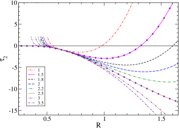
Figure 2: Second cluster integral $\tau_{2}$ for the 12-6 LJ system confined by a spherical wall. Each curve corresponds to a different temperature.

As an example of the obtained results in Fig. 2 we plot the dependence with $R$ of the second cluster integral for the 12-6 LJ fluid confined in a spherical pore. Curves show the asymptotic expression for large $R$, including terms of order $\mathcal{O}(R^{-18})$ (order $\varepsilon^{3}$ in $d_{2}$). Dots show numerical evaluation of the exact integral $\tau_{2}$. The highest considered $T$ is near to the Boyle temperature for $b_{2}$ therefore in this case $\tau_{2}$ is driven by $a_{2}A$. For very small radius exact results smoothly goes to zero. Yet, for $R\lesssim 0.6$ curves differ significantly form the exact results and isotherms of smaller temperature separates at higher radii from the exact result. We observed a similar behavior for other values of $k>6$ which do not include the logarithmic dependence with $R$.

V Results

Before analyzing the consequences on the LJ system of the obtained expressions for $\tau_{2}$, it is interesting to discuss in the present context some general relations known as exact sum rules. Once the volume notion is introduced, a further step in the thermodynamic interpretation of the confined system can be done. Starting from $\Omega$ we obtain the pressure that the system makes on the surrounding walls, the pressure on the wall $P_{\textrm{w}}$, that is the key magnitude of the reversible work term in the first law of thermodynamics. For systems confined by constant-curvature walls and using the volume notion defined in Sec. III $P_{\textrm{w}}$ is

$$P_{\textrm{w}} = -\frac{dR}{dV}\left.\frac{\partial\Omega}{\partial R}\right|_{\mu,T}\>.$$ (57)

The relation between $P_{\textrm{w}}$, $T$ and $z$ is the basic EOS of these inhomogeneous systems. It is not necessary to deal with bulk or surface properties. A second exact relation valid for constant-curvature hard confinement is

$$P_{\textrm{w}}=\rho_{\textrm{c}}T,$$ (58)

which is a contact theorem with $\rho_{\textrm{c}}=\rho(r=R)$. Both exact relations (57) and (58) are a convenient starting point to analyze the system properties.

For the three geometrical constraints we decompose $\Omega$ in Eq. (1) as

$$\Omega=-PV+\gamma A\>,$$ (59)

with bulk pressure $P=-\left.\frac{\partial\Omega}{\partial V}\right|_{\mu,T,A,R}$ and fluid-substrate surface tension $\gamma=\left(\Omega+PV\right)/A$. This definition identifies the fluid-substrate surface tension with an excess of free energy (over bulk and per unit area), but it is not the unique possible definition that can be adopted (for example $\left.\frac{\partial(\Omega+PV)}{\partial A}\right|_{\mu,T,V}$ is also sometimes used). Given that $\Omega$ and $P$ are the actual exact grand free-energy of the system and pressure of the reservoir at the same temperature and chemical potential, $\gamma$ defined in Eq. (59) strongly depends on the adopted measures of volume and surface area to describe the system properties. Mapping the results between different conventions may be done with a little of linear algebra.Urrutia (2014)

Once the decomposition of $\Omega$ in Eq. (59) is assumed there is a third exact sum rule that applies to spherical and cylindrical confined system

$$\Delta P = \gamma\frac{sc}{R}+\left.\frac{\partial\gamma}{\partial R}\right|_{\mu,T}\>,$$ (60)

where $\Delta P=\pm\left(P_{\textrm{w}}-P\right)$. Plus sign applies to the case of fluid in the outer region while minus sign applies to opposite. The parameter $sc$ is: $sc=2$ if the surface is a sphere, $sc=1$ for the cylinder. To include planes one may consider $sc=0$. Eq. (60) is the exact form that takes the Laplace equation in this context. In the case of the LJ fluid our expression of $\tau_{2}(R)$ enables to analytically evaluate $\Omega$, $P_{\textrm{w}}$, $\rho_{\textrm{c}}$ and $\gamma$ up to order $z^{2}$.

V.1 Low density inhomogeneous gas

We consider the unconstrained open system [$m\rightarrow\infty$ in Eq. (1)] of LJ particles at low density confined by planar, spherical or cylindrical walls. Then, we truncate Eq. (5) at second order to obtain $\beta\Omega=-zV-z^{2}\frac{1}{2}\tau_{2}$. Therefore the first consequence of our calculus on $\tau_{2}$ is that grand-free energy of 2$k$-$k$ LJ fluid contains the expected terms linear with volume and surface area. These terms are identical for the three studied geometries. At planar geometry, no extra term exist as symmetry implies for all $\tau_{i}$. In case of spherical confinement a term linear with total normal curvature of the surface $A2/R\propto R$ does not appear at order $z^{2}$ but it should exist at higher ones. A term linear with total Gaussian curvature $A/R^{2}\propto\textrm{constant}$ exist. Extra terms that scales with negative powers of $R$ were also found. A logarithmic term proportional to $\ln R^{-1}$ was recognized only for $k=6$. The cylindrical confinement is not very different to the spherical case. We simply trace the differences: even that Gaussian curvature is zero in this geometry, a term linear with $A/R^{2}\propto L/R$ was found. The existence of a logarithmic term for $k=6$ was verified, in this case it was proportional to $L\ln R^{-1}/R$.

Up to order $z^{2}$ we found the series expansions

$$\beta\Omega = -(z+z^{2}b_{2})V-z^{2}\frac{1}{2}\Delta\tau_{2}\>,$$

$$\beta P_{\textrm{w}} = z+z^{2}b_{2}+\frac{z^{2}}{2}A^{-1}\partial\Delta\tau_{2}/\partial R\>,$$

$$\rho_{\textrm{c}} = z+z^{2}2b_{2}+z^{2}2\Delta b_{2}(u=0)\>.$$ (61)

Last two relations through Eq. (58) imply $2\Delta b_{2}(u=0)=-b_{2}+A^{-1}\partial\Delta\tau_{2}/\partial R$. Furthermore, for bulk homogeneous system we found $\beta P=z+z^{2}b_{2}$ and $\rho_{\textrm{b}}=z+z^{2}2b_{2}$ (subscript b refers to the bulk at the same $T$ and $\mu$ conditions).

For the low density LJ fluid we obtainedUrrutia (2014)

$$\beta\gamma=-\frac{\Delta\tau_{2}}{2A}z^{2}=-\frac{\Delta\tau_{2}}{2A}\rho_{\textrm{b}}^{2}\>,$$ (62)

that are exact up to $\mathcal{O}(z^{3})$ and $\mathcal{O}(\rho_{\textrm{b}}^{3})$. For planar, spherical and cylindrical walls it reduces to

$$\gamma=a_{2}T\rho_{\textrm{b}}^{2}\>,\>\>\gamma=\left(a_{2}-\frac{c_{2}+d_{2}}{4\pi R^{2}}\right)T\rho_{\textrm{b}}^{2}\>,$$ (63)

$$\gamma=\left(a_{2}-\frac{3}{32\pi R^{2}}c_{2}+...\right)T\rho_{\textrm{b}}^{2}\>,$$ (64)

respectively. In Eq. (64) higher order terms are: $\mathcal{O}(R^{-4})$ for $k>6$, but includes terms $\mathcal{O}(R^{-2})$ if $k=6$ (even, it is exact up to order $R^{-2}\ln R$). Thus, results of Eqs. (48) to (52) enable us for the first time to study on analytic grounds the wall-fluid surface tension of the LJ systems for planar, spherical and cylindrical walls, at low density.

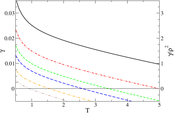
Figure 3: Surface tension of a 2$k$-$k$ LJ fluid in contact with a planar wall, we fix $\rho_{\textrm{b}}=0.1$ and consider various $k$ values. From top to bottom $k$ increases. Curves correspond to $k=6,7,8,9,12,18$.

In Fig.3 it is shown the surface tension of the 2$k$-$k$ LJ gas confined by a planar wall for different values of $k$. All cases show a monotonous decreasing behavior of $\gamma$ with $T$. At low temperatures $\gamma$ is positive (it diverges as $\exp(1/T)$ as $T\rightarrow 0$) and becomes negative at high temperatures. The temperature where $\gamma$ is zero is lower for bigger $k$ (temperatures are given in Tab. 1, second row). In the case of the 12-6 LJ system we found $\gamma\approx 0.035$ at $T=0.5$ and $\gamma\approx 0.01$ at $T=5$ ($\rho_{\textrm{b}}=0.1$). Scale on the right shows $\gamma/\rho_{\textrm{b}}^{2}$ which is independent of density.

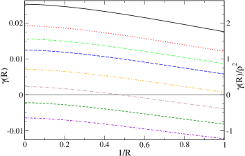
Figure 4: Surface tension of the 12-6 LJ fluid in contact with a spherical wall at $\rho_{\textrm{b}}=0.1$ (for both concave and convex shapes) and at various temperatures. From top to bottom $T=1,2,3,4,6,8,10,12$.

In the case of the spherical-wall the curvature dependence of the surface tension is plotted in Fig. 4. There, results for the 12-6 system at different temperatures are shown. At $T\apprge 9$ fluid-wall surface tension is negative even at $R\rightarrow\infty$. This negative sign of $\gamma$ is characteristic of systems with repulsive interaction such as the hard sphere fluid. Fig. 4 is also related with the excess surface adsorption $\Gamma=\left(<n>-<n>_{\textrm{b}}\right)/A$. Series expansion of $\Gamma$ up to order $z^{2}$ and $\rho_{\textrm{b}}^{2}$ are: $\Gamma=z^{2}\Delta\tau_{2}/A$$=\rho_{\textrm{b}}^{2}\Delta\tau_{2}/A$, respectively. Thus, up to the order of Eq. (63) it is $\Gamma=-2\gamma/T$. This shows that isotherms of $\gamma(R)$ shown in Fig. 4 also plot isotherms of $-\Gamma T/2$. Naturally, the same apply to the planar case shown in Fig.3 and to the cylindrical one (not shown).

It must be noted that $\gamma(R)$ and $\Gamma$ depend on the adopted surface of tension that we fixed at $r=R$ where $\rho(r)$ drops to zero. This fixes the adopted reference region characterized by measures $V$, $A$ and $R$. The effect of introducing a different reference region on $\gamma(R)$ was systematically studied in Refs. Urrutia (2014, 2015) for the hard-sphere fluid and the same approach applies to the LJ fluid.

Figure 5: Curvature dependent surface tension scaled with the inverse temperature. Continuous line shows our result [Eq. (62)], dashed line was extracted from Ref. Stewart and Evans (2005b). Other curves are described in the text.

Stewart and Evans studied the interfacial properties of a hard spherical cavity immersed in a fluid using effective interfacial potentials and density functional theory. They used an interaction potential between particles that contains both a hard sphere repulsion and an attractive $-r^{-6}$ component, the latter similar to that appearing in the 12-6 LJ potential.Stewart and Evans (2005b) In Fig. 3 therein it was presented a plot of $\beta\gamma$ as a function of $R^{-1}$ at $T=0.991$ and $\rho=0.018$. For comparison we present in Fig. 5 the curve found by Stewart and Evans (dashed) and our results for the 12-6 LJ gas obtained using Eq. (62) at the same temperature and density (continuous). We observe an overall discrepancy of $\sim 10\%$ which is acceptable by virtue of the disparity in the interaction model. Two major differences between both curves account most of the observed discrepancy. On the one hand, the ordinate at the origin i.e. the value of surface tension in the limit of planar wall. On the other hand, the slope of curves at $R^{-1}\rightarrow 0$ which is not zero for dashed curve. The difference in the observed planar-wall surface tension is a direct consequence of the disparity in the interaction model. Even though, the difference in the slope is produced by our second order truncation that forces a zero slope. In dot-dashed we present a version of dashed line compensated to give $\delta(R^{-1}\rightarrow 0)=0$. This last line was shifted an arbitrary value and plotted in dot-dot-dashed to make clear the coincidence with the obtained virial series result. In this case the shape is identical which suggest that $\ln R/R^{2}$ and $R^{-2}$ terms are not susceptible to the disparity of potentials.

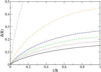
Figure 6: Radius dependent Tolman length of the 12-6 LJ fluid in contact with a spherical wall (for both concave and convex shapes) and at various temperatures. From bottom to top $T=1,2,3,4,6,8$.

The fluid-substrate radius dependent Tolman Length, defined by $\delta(R)=\frac{R}{2}\left[1-\frac{\gamma(R)}{\gamma}\right]$, measures the dependence of the surface tension with the curvature. For all temperatures we found a positive $\delta(R)$, that goes to zero at the planar limit and increases monotonously with $R^{-1}$. Curve for $T=8$ increases monotonously until reaches the value $\delta(1)=1.33$. Note that at Boile temperature $T=9.016$ where $\gamma$ goes to zero $\delta(R)$ diverges.

V.2 Curvature expansion

We follow Ref. Blokhuis and van Giessen (2013) to analyze the curvature expansion of the surface tension. There, the analysis was done for the vapor fluid interface. HelfrichHelfrich (1973) gives an expansion of the surface tension in the curvature up to second order. Applied to the sphere and cylinder symmetry Helfrich expansion of $\gamma(R)$ gives

$$\gamma_{\textrm{s}}(R) = \gamma-\frac{2\delta\gamma}{R}+\frac{2\boldsymbol{k}+\bar{\boldsymbol{k}}}{R^{2}}+\ldots\>,$$ (65)

$$\gamma_{\textrm{c}}(R) = \gamma-\frac{\delta\gamma}{R}+\frac{\boldsymbol{k}}{2R^{2}}+\ldots\>,$$ (66)

where dots represent terms of $\mathcal{O}(R^{-3})$. The radius independent Tolman length is $\delta(R\rightarrow\infty)=\delta$. Next term beyond $\delta$ is related with the bending rigidity $\boldsymbol{k}$ related with the square of the total curvature and the Gaussian rigidity $\bar{\boldsymbol{k}}$ associated with Gaussian curvature. On the basis of our results expansion on Eqs. (65, 66) are adequate for $k>6$. Therefore, for $k>6$ we found $\delta=\mathcal{O}(\rho_{\textrm{b}}^{3})$,

$$\boldsymbol{k} = -\frac{\pi}{32k}C_{6/k}(0)\,T\,\rho_{\textrm{b}}^{2}+\ldots\>,$$ (67)

$$\bar{\boldsymbol{k}} = \frac{\pi}{48}C_{6/k}(0)\,T\,\rho_{\textrm{b}}^{2}+\ldots\>,$$ (68)

where dots represent terms of order $\mathcal{O}(\rho_{\textrm{b}}^{3})$. Note that even at order $\rho_{\textrm{b}}^{2}$ both rigid constants have a non trivial dependence on $T$. It is interesting to calculate the quotient between $\boldsymbol{k}$ and $\bar{\boldsymbol{k}}$ which gives for all $k>6$

$$\boldsymbol{k}/\bar{\boldsymbol{k}}=-3/2\>.$$ (69)

Remarkably, it is a universal value in the sense that it is independent of both $k$ and the state variables $T$ and $\rho_{\textrm{b}}$. It is trivial to verify that this relation also applies to HS and SW particles.Urrutia (2014)

For long-ranged interactions as in the case of 12-6 LJ the existence of the discussed logarithmic terms makes the Helfrich expansionHelfrich (1973) of $\gamma(R)$ in power of $R^{-1}$ no longer valid. Thus, for $k=6$ instead of the Helfrich-based expression Eqs. (65, 66), one obtains for the spherical and cylindrical walls

$$\gamma_{\textrm{s}}(R) = \gamma-\frac{2\delta\gamma}{R}+\left(2\boldsymbol{k}+\bar{\boldsymbol{k}}\right)\frac{\ln R^{-1}}{R^{2}}+\ldots\>,$$ (70)

$$\gamma_{\textrm{c}}(R) = \gamma-\frac{\delta\gamma}{R}+\boldsymbol{k}\frac{\ln R^{-1}}{2R^{2}}+\ldots\>.$$ (71)

Here dots represent terms of $\mathcal{O}(R^{-2})$. Again, bending and Gaussian rigidities were identified with the next order terms beyond $\delta$. We obtain for the series expansion beyond the null Tolman length

$$\boldsymbol{k}=\frac{\pi}{8}\rho_{\textrm{b}}^{2}+\ldots\>\>\>\textrm{ and }\>\>\>\bar{\boldsymbol{k}}=-\frac{\pi}{12}\rho_{\textrm{b}}^{2}+\ldots\>\>,$$ (72)

where dots represent terms of order $\mathcal{O}(\rho_{\textrm{b}}^{3})$. In this case both rigidities are temperature independent. Even for $k=6$ the quotient gives the same result $\boldsymbol{k}/\bar{\boldsymbol{k}}=-3/2$, found in Eq. (69). In fact, the origin of this fundamental value is purely geometrical and lies in Eq. (35). Expressions identical to those given in Eq. (72), but with the difference between bulk densities in liquid and vapor phases instead of $\rho_{\textrm{b}}$, were found previously for the free liquid-vapor interface of the full (uncut) 12-6 LJ fluid.Blokhuis and van Giessen (2013)

Thus, essentially any pair interacting potential, including all the finite range potentials (e.g. the cut and shifted 12-6 LJ, HS, SW and square-shoulder, potentials) produce the same value for the ratio $\boldsymbol{k}/\bar{\boldsymbol{k}}$ at low density. We also calculate the quotient of the next to $R^{-1}$ terms between spherical and cylindrical cases, the ratio $\left(2\boldsymbol{k}+\bar{\boldsymbol{k}}\right)/\left(\boldsymbol{k}/2\right)=-8/3$. Again it has a purely geometrical origin and has the advantage of being independent of the assumptions of a Helfrich-based expression for $\gamma(R)$. This result is in line with that found numerically using a (second-virial approximation) DFTReindl et al. (2015) for all the studied potentials: LJ, SW, square-shoulder and Yukawa, all of them cut at finite range. The same geometrical status claimed for $\boldsymbol{k}/\bar{\boldsymbol{k}}$ corresponds to the result $\delta=0+\mathcal{O}(\rho^{3})$ that is directly derivable from Eq. (16) and applies to essentially any pair potential.

Based on the Hadwiger theorem it was proposed that bending constant could be zero,König et al. (2005) and thus, is unnecessary to include it in the expansion of $\gamma(R)$. Eq. (69) shows that the inaccuracy introduced by truncation of the bending rigidity term in Eqs. (65, 66) is of the same order than the Gaussian rigidity term (at least for hard walls), and therefore is not well justified from the numerical standpoint.

VI Conclusions

We give a simple and concise presentation of statistical mechanics for inhomogeneous fluid systems that is appropriate to discuss virial series in powers of the activity. The advantage of the adopted framework is highlighted by showing short and explicit expressions of virial series for the free energy and one- and two-body distribution functions. Our approach, that avoids the introduction of a priori assumptions about the free energy is, in fact, a selection of different formulations and ideas taken from Bellemans, Sokolowski and Stecki, and Rowlinson, that we managed to assimilate and develop a synthetical representation.

Our point of view heightens the relevance of cluster integrals by their generalization to inhomogeneous fluid-type systems. These cluster integrals, that reduce to the Mayer ones in the case of homogeneous fluids, are the coefficients of the series expansion in the activity of the free energy. Extensions of the concept of cluster integral and cluster integrand enable us to analyze under the same approach the residual terms of distribution functions. Virial series in power of either the bulk and mean densities (the bulk density as in Bellemans approach, or the mean density of the system as adopted by Rowlinson) are thus considered as two of many possible choices for the independent variable in the power series representation of free energy. It should noted that expansions in the activity have shown to be simpler to analyze when different conventions for the reference region (its volume, area and shape) are utilized.Urrutia (2014, 2015)

Second order terms i.e. the second cluster integral and the second order residue of one particle distribution were analyzed in detail when the system is confined by hard walls of an arbitrary shape. To do so we incorporated the advances developed by Bellemans, Sokolowski and Stecki. By limiting the study cases of the applied external potential and the order of the expansion we were able to shift the load to the solution of cluster integrals. This is not minor since it reduces an originally general and quite hard to address framework to a more straightforward method. It should not be overlooked that the hypothesis leading to Eq. (19) for $\Delta\tau_{2}$ are common to a lot of systems of major interest, at least in an approximate manner. Then, $\Delta\tau_{2}$ equation becomes a rather powerful tool for tackling inhomogeneous systems in a wide spectrum, specially for direct numerical solving.

By analytically solving the simpler situations for $\Delta\tau_{2}$ we were able to expose the volume, area and other terms that contribute, acquiring the capacity to discriminate between bulk terms and a hierarchy of inhomogeneous terms that characterizes the curvature dependence. Particularly, we focused in confining regions with a constant curvature boundary: planar, spherical and cylindrical cases. As a simple application of our findings to a non-trivial problem, we analyzed the second cluster integral for the confined LJ system. We evaluated analytically the temperature and radius dependence of $\tau_{2}$ and $\left\llbracket\rho^{(2)}(\mathbf{r})\right\rrbracket$. The 12-6 LJ system was considered but also the more general 2$k$-$k$ LJ potential. It was found that second cluster integral of the 12-6 LJ system contains a bulk, a surface, and also a non-analytic dependence with $R$. The latter are, in a spherical confinement a $\ln R$ term and, in cylindrical confinement a $L\ln R/R$ term. For $k\geq 7$ these logarithmic dependencies are absent (sphere) or may appear at higher order in $R^{-1}$ (cylinder) but in all cases a series of terms proportional to negative powers of $R$ were also obtained. We obtained the free energy of the inhomogeneous systems by truncation of the virial series order at order $z^{2}$ and $\rho_{\textrm{b}}^{2}$, that directly maps our findings on $\tau_{2}$ to free energy. The existence of Log terms in the free energy of fluids in contact with hard spherical surfaces was hypothesized by Henderson and later discussed by Stecki and col. Henderson (1983); Stecki and Toxvaerd (1990); Poniewierski and Stecki (1997); Samborski et al. (1993). Our results demonstrate this conjecture for the 12-6 LJ system.

The fluid-substrate surface tension was also analyzed using second order truncated virial series. In the planar case we found an exact expression that describes $\gamma(T)$ for all $k\geq 6$. We evaluated the temperature below that the surface tension becomes negative. For $k=6$ it is $6.8\times T_{c}$. The prefactor decreases with $k$ being $2.2\times T_{c}$ for $k=18$ that corresponds to short range potentials proper of colloidal particles. Based on the virial series approach the leading order curvature correction to the surface tension $\gamma(R)$ for all the $2k$-$k$ LJ fluids in contact with spherical and cylindrical surfaces was found analytically, at order two in density. This correction is the same when the system is inside of the surface or outside of it. For $k=6$ in the case of both spherical and cylindrical confinement surface tension scales with $\ln R/R^{2}$. For the $k\geq 7$ the first correction is order $R^{-2}$. In all cases the correction is negative for high temperatures. The truncation of the 12-6 LJ potential produces a significant change in the dependence of $\gamma(R)$ with $R$, vanishing the $\ln R/R^{2}$ dependence and producing a simple correction. We observed that the term of order $R^{-1}$ is zero for $k\geq 6$. This shows that Tolman length is zero up to order $\rho_{\textrm{b}}^{2}$ but it should appear at higher order ones, probably at order $\rho_{\textrm{b}}^{3}$.

The curvature dependence of surface tension for fluid interfaces is a highly studied issue.Blokhuis and van Giessen (2013); Corti et al. (2011); Hansen-Goos (2014); Tröster et al. (2012); Baidakov et al. (2009); Wilhelmsen et al. (2015); Giessen and Blokhuis (2009); Blokhuis (2013); Urrutia (2014); Baidakov and Bobrov (2014) In particular, the amplitude and sign of bending and Gaussian rigidity constants are a matter of discussion. We evaluated analytically both rigidities, $\boldsymbol{k}$ and $\bar{\boldsymbol{k}}$, at order $z^{2}$ and $\rho_{\textrm{b}}^{2}$. For $k=6$ both bending and Gaussian rigidities are independent of temperature, being $\boldsymbol{k}>0$ and $\bar{\boldsymbol{k}}$<0. Other values of $k$ are characterized by a temperature where both rigidities change its sign. For all $k\geq 6$ we obtained the universal ratio $\boldsymbol{k}/\bar{\boldsymbol{k}}=-3/2$ which is a thermodynamic result based on pure geometrical grounds. This value is exact when terms of order $\rho_{\textrm{b}}^{3}$ are truncated from the EOS of the system. We obtain the same result for any finite range potential.

Previous works have discussed the existence of $\ln R$ non-analytic dependence of the surface tension with the curvature when dispersion forces are present and multiple techniques were used with this purpose including DFT, MonteCarlo, Molecular dynamics and effective Hamiltonian.Schmitz et al. (2014a, b) These terms were found at the gas-liquid interface of droplets and bubbles,Blokhuis and van Giessen (2013) and at the curved wall-fluid interface.Blokhuis and Kuipers (2007); Stewart and Evans (2005b) In wetting and drying at curved surfaces it was also identified.Evans et al. (2003, 2004); Stewart and Evans (2005a, b) In all those cases the magnitude of this term is indirectly evaluated: it may involve the truncation of the interaction potential, the fitting of density profiles and/or surface tension curves, the use of approximate EOS for the bulk system or more than one of this approximations. This yields results that require deeper testing. Our analytical approach is a contribution in that direction.

Appendix A Function $S(r,u)$ for cylindrical walls

The surface term $S(r,u)$ was evaluated by taking the derivative of the volume of intersection between a cylinder and a sphere which can be expressed in terms of elliptic integrals. For the case $0<r<2R$ we obtained

$$\begin{array}[]{c}S(r,u)=4\pi r^{2}\Theta(-u)+\frac{2r}{\sqrt{R(R+u)}}\left[-4R(R+u)E(Q)+\right.\\ \left(4R^{\text{2}}+2Ru-r^{2}\right)K(Q)+r^{2}\left(\frac{2R}{u}+1\right)\varPi\Bigl{(}1-\frac{r^{2}}{u^{2}},Q\Bigr{)}\Bigr{]}\>,\end{array}$$

with $Q=\frac{r^{2}-u^{2}}{4R(R+u)}$ and being $\Theta(x)$ the Heaviside step function which is $\Theta(x)=1$ if $x>0$ and $\Theta(x)=0$ otherwise. Also, $K(Q)$, $E(Q)$ and $\varPi(x,Q)$ are the complete elliptic integral of the first, second and third kind, respectively (here $Q$ is the parameter and $x$ the characteristic).Abramowitz and Stegun (1972) Note that $S(r,u)$ is a smooth function at $u=0$, because the discontinuity in $\Theta(-u)$ compensates with a discontinuity in $\varPi\Bigl{(}1-\frac{r^{2}}{u^{2}},Q\Bigr{)}$. We analyzed the behavior of $S(r,u)$ at large $R$ value by taking its series expansion. For the case $r>2R$ we found

$$\begin{array}[]{c}S(r,u)=4\pi r^{2}\Theta(u)+\frac{4r}{\sqrt{r^{2}-u^{2}}}\biggl{\{}(u^{2}-r^{2})E\!\left(\frac{1}{Q}\right)+\\ (2R-u)\biggl{[}u\,K\!\left(\frac{1}{Q}\right)-\frac{r^{2}}{u}\varPi\!\Bigl{(}\frac{4R(u-R)}{u^{2}},\frac{1}{Q}\Bigr{)}\biggr{]}\biggr{\}}\>.\end{array}$$

Appendix B Functions $I_{\nu,\varepsilon}$ and $C_{q}$

Here we analyzed function $I_{\nu,\varepsilon}$ focusing on its behavior at small $\varepsilon$. For $\nu<1$ $\underset{\varepsilon\rightarrow 0}{\lim}I_{\nu,\varepsilon}$ converges to

$$I_{\nu} = \frac{1}{2}z^{\left(\nu+1\right)/2}\left[\Gamma\left(\frac{1-\nu}{2}\right){}_{1}F_{1}\left(\frac{1-\nu}{2},\frac{1}{2},\frac{z}{4}\right)+\right.$$ (73)

$$\left.\sqrt{z}\,\Gamma\left(1-\frac{\nu}{2}\right){}_{1}F_{1}\left(1-\frac{\nu}{2},\frac{3}{2},\frac{z}{4}\right)\right]\>,$$

where ${}_{1}F_{1}\left(a,b,x\right)$ is the Kummer’s hypergeometric function. For this case we find the series expansion

$$I_{\nu,\varepsilon}=I_{\nu}+z\varepsilon^{1-\nu}\!\Bigl{(}\frac{1}{\nu-1}\!+\!\frac{z\varepsilon}{\nu-2}\!+\!\frac{z\varepsilon^{2}(z-2)}{2(\nu-3)}\!+\!\ldots\Bigr{)}$$ (74)

Otherwise, if $\nu\geq 1$ then $\underset{\varepsilon\rightarrow 0}{\lim}I_{\nu,\varepsilon}$ diverges. $I_{1,\varepsilon}$ has been split in a divergent term, $z\int_{\varepsilon}^{\infty}u^{-1}\exp\left(-zu^{2}\right)du$, and a non-divergent term, both have been evaluated separately to obtain

$$I_{1,\varepsilon} = -\frac{z}{2}\Bigl{[}\ln\left(z\varepsilon^{2}\right)+\gamma_{e}-{}_{1}F_{1}^{(1,0,0)}\left(0,\frac{1}{2},\frac{z}{4}\right)-$$ (75)

$$\!\!\!\!\pi\text{Erfi}\left(\frac{\sqrt{z}}{2}\right)\Bigr{]}-\varepsilon z^{2}+\varepsilon^{2}\left(\frac{z^{2}}{2}-\frac{z^{3}}{4}\right)+\ldots$$

Here, $\gamma_{e}$ is the Euler gamma constant, Erfi$(x)$ is the imaginary error function and ${}_{1}F_{1}^{(1,0,0)}(0,b,z)$ is $\partial{}_{1}F_{1}(a,b,z)/\partial a$ evaluated at $a=0$ [which is equivalent to ${}_{1}F_{1}^{(1,0,0)}(0,b,x)=b^{-1}x\,{}_{2}F_{2}(1,1;b+1,2;x)$]. For $\nu\neq 0$ we obtained the recurrence relation

$$\frac{\nu}{z}I_{\nu+1,\varepsilon}=\varepsilon^{-\nu}\exp\left[-z\left(\varepsilon^{2}-\varepsilon\right)\right]+I_{\nu,\varepsilon}-2I_{\nu-1,\varepsilon}\>,$$ (76)

which combined with Eqs. (74) and (75) enables to obtain the expansion of $I_{\nu,\varepsilon}$ for any real value $\nu>1,$ that completes our procedure to obtain $I_{\nu,\varepsilon}$ with $\nu\in\mathbb{R}$. For $\nu>1$ Eq. (76) shows that the divergence is driven by $I_{\nu,\varepsilon}\sim\frac{z\varepsilon^{1-\nu}}{\nu-1}$.

For $0<q<1$ $\underset{\varepsilon\rightarrow 0}{\lim}C_{q}(\varepsilon)$ converges to

$$C_{q}(0) = \frac{z^{q/2}}{2}\left[\Gamma\left(-\frac{q}{2}\right){}_{1}F_{1}\left(-\frac{q}{2},\frac{1}{2},\frac{z}{4}\right)+\right.$$ (77)

$$\left.\sqrt{z}\,\Gamma\left(\frac{1-q}{2}\right){}_{1}F_{1}\left(\frac{1-q}{2},\frac{3}{2},\frac{z}{4}\right)\right]\>,$$

and the series expansion for $C_{q}(\varepsilon)$ is

$$C_{q}(\varepsilon)=C_{q}(0)+z\varepsilon^{1-q}\!\left(\frac{1}{q-1}+\frac{(z-2)\varepsilon}{2(q-2)}+\frac{z(z-6)\varepsilon^{2}}{6(q-3)}+...\right).$$ (78)

For $q=1$ we separated second term of Eq. (43) in several terms and evaluated each of them, we found

$$C_{1}(\varepsilon) = -z\ln(\sqrt{z}\varepsilon)-\sqrt{\pi}\sqrt{z}e^{z/4}\left[1+\text{Erf}\left(\frac{\sqrt{z}}{2}\right)\right]+$$ (79)

$$\frac{z}{2}\!\left[2-\gamma_{e}+\pi\text{Erfi}\!\left(\frac{\sqrt{z}}{2}\right)+{}_{1}F_{1}^{(1,0,0)}\!\!\left(0,\frac{1}{2},\frac{z}{4}\right)\right]\!+$$

$$\left(1-\frac{z}{2}\right)z\varepsilon+\frac{6-z}{12}z^{2}\varepsilon^{2}+\mathcal{O}\left(\varepsilon^{3}\right)\>,$$

where the divergent term is $-z\ln(\sqrt{z}\varepsilon)$ and Erf$(x)$ is the error function. For $q>1$ we used the simple relation $C_{q}(\varepsilon)=-\frac{1}{q}\varepsilon^{-q}+\frac{1}{z}I_{q+1,\varepsilon}$ (valid for $q>0$) to obtain the following recurrence relation

$$qC_{q}(\varepsilon) = \varepsilon^{-q}\left\{\exp\left[-z\left(\varepsilon^{2}-\varepsilon\right)\right]-1+\frac{z\varepsilon}{q-1}\right\}+$$ (80)

$$zC_{q-1}(\varepsilon)-2I_{q-1,\varepsilon}\>.$$

This relation joined with Eqs. (78, 79) allow to obtain the expansion of $C_{q}(\varepsilon)$ for all $q>0$. Eq. (80) shows that the divergence of $C_{q}(\varepsilon)$ for $q>1$ is driven by $C_{q}(\varepsilon)\sim\frac{zq}{q-1}\varepsilon^{1-q}$. Finally, we found the following interesting property:

$$\underset{q\rightarrow 0}{\lim}\>qC_{q}(0)=-1\>,$$ (81)

for all $z>0$ (finite values of $T$) that is used in Sec. IV.1 to study the conditions under which LJ systems behaves as HS.

Appendix C Coefficients for cylindrical walls

For cylindrical walls we also analyzed separately the cases $k>6$ and $k=6$. If $k>6$, $x_{2}$ is proportional to $c_{2}$ [see Eqs. (35, 49)] and

$$d_{2} = -\frac{V2\pi}{k}\Delta C_{3/k}+\frac{A\pi}{2k}\Delta C_{4/k}-\frac{L}{R}\frac{\pi^{2}}{32k}\Delta C_{6/k}+$$

$$\frac{L}{R^{3}}\frac{\pi^{2}}{1024k}C_{8/k}+\ldots$$

with a series expansion $d_{2}\approx L(2R)^{5-k}$. The coefficient of this main term in $d_{2}$ was left unevaluated because higher order functions contribute to this order. The case $k=8$ requires a special attention because its series gives $d_{2}\approx L\ln R/R^{3}$.

If $k=6$,

$$\tilde{x}_{2} = -\frac{V\pi}{3}\Delta C_{1/2}+\frac{A\pi}{12}\Delta C_{2/3}+\frac{L}{R}\frac{\pi^{2}}{192}C_{1}(\varepsilon)+$$

$$\frac{L}{R^{3}}\frac{\pi^{2}}{1024k}C_{4/3}+\ldots$$

Note that $R^{-3}C_{4/3}(\varepsilon)\approx R^{-1}$ and the same occurs with higher order terms like $R^{-5}C_{5/3}(\varepsilon)\approx R^{-1}$. Therefore, we truncated $\tilde{x}_{2}$ to this order which results in the expression for $x_{2}$ written in Eq. (53) and leaves $d_{2}$ unevaluated.