EUROPEAN ORGANIZATION FOR NUCLEAR RESEARCH (CERN)

​​​ CERN-EP-2016-047 LHCb-PAPER-2016-002 June 6, 2016

Observation of the ${{\mathchar 28931\relax}^{0}_{b}}\rightarrow{\mathchar 28931\relax}\phi$ decay

The LHCb collaboration

The ${{\mathchar 28931\relax}^{0}_{b}}\rightarrow{\mathchar 28931\relax}\phi$ decay is observed using data corresponding to an integrated luminosity of 3.0$\mbox{\,fb}^{-1}$ recorded by the LHCb experiment. The decay proceeds at leading order via a ${b}\rightarrow{{s}{\overline{s}}}{s}$ loop transition and is therefore sensitive to the possible presence of particles beyond the Standard Model. A first observation is reported with a significance of $5.9$ standard deviations. The value of the branching fraction is measured to be $(5.18\pm 1.04\pm 0.35\,^{+0.67}_{-0.62})\times 10^{-6}$, where the first uncertainty is statistical, the second is systematic, and the third is related to external inputs. Triple-product asymmetries are measured to be consistent with zero.

Published in Phys. Lett. B759 (2016) 282

© CERN on behalf of the LHCb collaboration, licence CC-BY-4.0.

 

1 Introduction

In the Standard Model (SM), the flavour-changing neutral current decay ${{\mathchar 28931\relax}^{0}_{b}}\rightarrow{\mathchar 28931\relax}\phi$ proceeds via a ${b}\rightarrow{{s}{\overline{s}}}{s}$ loop (penguin) process. A Feynman diagram of the gluonic penguin that contributes to this decay at leading order is displayed in Fig. 1. This transition has been the subject of theoretical and experimental interest in ${B}^{0}_{s}$ and ${B}^{0}$ decays, since possible beyond the SM particles in the loop could induce non-SM $C\!P$ violation [1, 2, 3]. The process has been probed with decay-time-dependent methods in the ${{B}^{0}_{s}}\rightarrow\phi\phi$ and ${{{B}^{0}}\!\rightarrow{{K}^{0}_{\mathrm{\scriptscriptstyle S}}}\phi}$ decay modes [4, 5, 6, 7], which test for $C\!P$ violation in the interference between mixing and decay. In addition, measurements of $C\!P$ violation in the decay have been performed with the flavour-specific ${{B}^{0}}\!\rightarrow{{K}^{*0}}\phi$ channel [8]. The results to date are consistent with $C\!P$ conservation in the ${b}\rightarrow{{s}{\overline{s}}}{s}$ process. Model-independently, non-SM physics contributions could appear differently in these decay modes, though many models contain strong correlations [9].

Figure 1: Feynman diagram contributing to the ${{\mathchar 28931\relax}^{0}_{b}}\rightarrow{\mathchar 28931\relax}\phi$ decay.

Measurements with ${\mathchar 28931\relax}^{0}_{b}$ baryons offer the possibility to look for $C\!P$ violation in the decay, both by studying $C\!P$ asymmetries and by means of $T$-odd observables. These observables have been studied in greater detail for ${B}^{0}_{s}$ and ${B}^{0}$ meson decays than those for ${\mathchar 28931\relax}^{0}_{b}$ baryons [10, 11, 4, 8]. Proposed methods to study $T$-odd asymmetries of ${\mathchar 28931\relax}^{0}_{b}$ baryons [12] exploit the polarisation structure of ${{\mathchar 28931\relax}^{0}_{b}}\rightarrow{\mathchar 28931\relax}V$ decays, where $V$ denotes a vector resonance [12], and can be affected by the initial ${\mathchar 28931\relax}^{0}_{b}$ polarisation if non-zero. An LHCb measurement of the initial polarisation in ${{\mathchar 28931\relax}^{0}_{b}}\!\rightarrow{{J\mskip-3.0mu/\mskip-2.0mu\psi\mskip 2.0mu}}{\mathchar 28931\relax}$ decays has yielded a value consistent with zero, though polarisation at the level of $10\%$ is possible given statistical uncertainties [13]. No SM prediction exists specifically for the $T$-odd asymmetries in ${{\mathchar 28931\relax}^{0}_{b}}\!\rightarrow{\mathchar 28931\relax}\phi$ decays, though no large asymmetries are expected given the prediction of $C\!P$ conservation in the decays of beauty mesons for the same transition. Measurements of $C\!P$ asymmetries have been performed by LHCb in an inclusive analysis of ${{\mathchar 28931\relax}^{0}_{b}}\rightarrow{\mathchar 28931\relax}hh^{\prime}$ decays [14], where $h(h^{\prime})$ refers to a kaon or pion, with corresponding $C\!P$ asymmetries measured to be consistent with zero.

In this paper, a measurement of the ${{\mathchar 28931\relax}^{0}_{b}}\!\rightarrow{\mathchar 28931\relax}\phi$ branching fraction is presented using the ${{B}^{0}}\!\rightarrow{{K}^{0}_{\mathrm{\scriptscriptstyle S}}}\phi$ decay as a normalisation channel, which has a measured branching fraction of $(7.3^{+0.7}_{-0.6})\times 10^{-6}$ [15]. The selection requirements used to isolate the ${{\mathchar 28931\relax}^{0}_{b}}\!\rightarrow{\mathchar 28931\relax}\phi$ decay with well-understood efficiencies reject suitable control channels for a $\Delta A_{{C\!P}}$ measurement. The ${{\mathchar 28931\relax}^{0}_{b}}\!\rightarrow{\mathchar 28931\relax}\phi$ sample is then used to perform measurements of the $T$-odd triple-product asymmetries, which do not require a control channel. The results are based on $pp$ collision data corresponding to an integrated luminosity of $1.0\mbox{\,fb}^{-1}$ and $2.0\mbox{\,fb}^{-1}$ collected by the LHCb experiment at centre-of-mass energies of $\sqrt{s}=7\mathrm{\,Te\kern-1.00006ptV}$ in 2011 and 8$\mathrm{\,Te\kern-1.00006ptV}$ in 2012, respectively.

2 Detector and simulation

The LHCb detector [16, 17] is a single-arm forward spectrometer covering the pseudorapidity range $2<\eta<5$, designed for the study of particles containing $b$ or $c$ quarks. The detector includes a high-precision tracking system consisting of a silicon-strip vertex detector surrounding the $pp$ interaction region, a large-area silicon-strip detector located upstream of a dipole magnet with a bending power of about $4{\mathrm{\,Tm}}$, and three stations of silicon-strip detectors and straw drift tubes placed downstream of the magnet. The tracking system provides a measurement of momentum, $p$, of charged particles with a relative uncertainty that varies from 0.5% at low momentum to 1.0% at 200${\mathrm{\,Ge\kern-1.00006ptV\!/}c}$. The minimum distance of a track to a primary vertex, the impact parameter, is measured with a resolution of $(15+29/\mbox{$p_{\mathrm{T}}$}){\,\upmu\mathrm{m}}$, where $p_{\mathrm{T}}$ is the component of the momentum transverse to the beam, in ${\mathrm{\,Ge\kern-1.00006ptV\!/}c}$. Different types of charged hadrons are distinguished using information from two ring-imaging Cherenkov detectors. Photons, electrons and hadrons are identified by a calorimeter system consisting of scintillating-pad and preshower detectors, an electromagnetic calorimeter and a hadronic calorimeter. The online event selection is performed by a trigger, which consists of a hardware stage, based on information from the calorimeter and muon systems, followed by a software stage, which applies a full event reconstruction. At the hardware trigger stage, events are required to have a muon with high $p_{\mathrm{T}}$ or a hadron, photon or electron with high transverse energy in the calorimeters. For hadrons, the transverse energy threshold is 3.5$\mathrm{\,Ge\kern-1.00006ptV}$. In the subsequent software trigger, at least one charged particle must have a transverse momentum $\mbox{$p_{\mathrm{T}}$}>1.7$${\mathrm{\,Ge\kern-1.00006ptV\!/}c}$ and be inconsistent with originating from a PV. Finally, the tracks of two or more of the final-state particles are required to form a vertex that is significantly displaced from the PVs. The final state particles that are identified as kaons are required to have a combined invariant mass consistent with that of the $\phi$ meson.

In the simulation, $pp$ collisions are generated using Pythia8 [18, *Sjostrand:2007gs] with a specific LHCb configuration [20]. Decays of hadronic particles are described by EvtGen [21], in which final-state radiation is generated using Photos [22]. The interaction of the generated particles with the detector, and its response, are implemented using the Geant4 toolkit [23, *Agostinelli:2002hh] as described in Ref. [25]. The decays of ${\mathchar 28931\relax}^{0}_{b}$ baryons are modelled according to a phase-space description. Differences in the efficiencies of protons and anti-protons, at the sub-percent level, are accounted for with the Geant4 implementation of the detector description.

3 Selection

The ${{{\mathchar 28931\relax}^{0}_{b}}\!\rightarrow{\mathchar 28931\relax}\phi}$ and ${{{B}^{0}}\!\rightarrow{{K}^{0}_{\mathrm{\scriptscriptstyle S}}}\phi}$ decays are reconstructed through the ${\mathchar 28931\relax}\rightarrow{p}{{\pi}^{-}}$, ${{K}^{0}_{\mathrm{\scriptscriptstyle S}}}\rightarrow{{\pi}^{+}}{{\pi}^{-}}$ and $\phi\rightarrow{{K}^{+}}{{K}^{-}}$ final states, where the inclusion of charge conjugate processes is implied throughout the paper. Decays of ${\mathchar 28931\relax}\!\rightarrow{p}{{\pi}^{-}}$ and ${{K}^{0}_{\mathrm{\scriptscriptstyle S}}}\!\rightarrow{{\pi}^{+}}{{\pi}^{-}}$ are reconstructed in two different categories. The first category contains $\mathchar 28931\relax$ (${K}^{0}_{\mathrm{\scriptscriptstyle S}}$) hadrons that decay inside the vertex detector acceptance and the second contains $\mathchar 28931\relax$ (${K}^{0}_{\mathrm{\scriptscriptstyle S}}$) hadrons that decay outside. These categories are referred to as long and downstream, respectively. The high resolution of the vertex detector leads to enhanced momentum, vertex, and mass resolutions for candidates in the long category relative to downstream candidates.

Boosted decision trees (BDTs) [26, 27] are used to separate signal from background. Different BDTs are trained for decays where the daughter tracks of the ${\mathchar 28931\relax}$ (${K}^{0}_{\mathrm{\scriptscriptstyle S}}$) hadron are classified as long or downstream and according to whether the data was collected in 2011 (7$\mathrm{\,Te\kern-1.00006ptV}$) or 2012 (8$\mathrm{\,Te\kern-1.00006ptV}$), yielding eight separate BDTs in total. The set of input variables used to train the ${{\mathchar 28931\relax}^{0}_{b}}\!\rightarrow{\mathchar 28931\relax}\phi$ (${{B}^{0}}\!\rightarrow{{K}^{0}_{\mathrm{\scriptscriptstyle S}}}\phi$) BDTs consists of the ${\mathchar 28931\relax}^{0}_{b}$ (${B}^{0}$) vertex fit quality, $p_{\mathrm{T}}$, $\eta$, the difference in $\chi^{2}$ of the PV reconstructed with and without the candidate ($\chi^{2}_{\rm IP}$), the flight distance squared divided by the associated variance ($\chi^{2}_{\rm FD}$), the angle between the momentum vector and the vector from the PV to the decay vertex, the ${\mathchar 28931\relax}$ (${K}^{0}_{\mathrm{\scriptscriptstyle S}}$) vertex fit quality, and the $p_{\mathrm{T}}$ and $\eta$ of the $\phi$ and the ${\mathchar 28931\relax}$ (${K}^{0}_{\mathrm{\scriptscriptstyle S}}$) hadrons. The minimum and maximum values of the $p_{\mathrm{T}}$ and $\eta$ associated to the final state particles are also included. In addition, the BDT trained on the long category uses the $\chi^{2}_{\rm IP}$ and $\chi^{2}_{\rm FD}$ of the ${\mathchar 28931\relax}$ (${K}^{0}_{\mathrm{\scriptscriptstyle S}}$) with respect to the associated PV. A PV is reconstructed by requiring a minimum of five good quality tracks that are consistent with originating from the same location within the luminous region. Before the BDTs are trained, initial loose requirements are imposed on the input variables. The BDTs are trained using simulated candidates for the signal and data sidebands for the background. For the training samples, the signal region is defined as being within 150${\mathrm{\,Me\kern-1.00006ptV\!/}c^{2}}$ of the known ${\mathchar 28931\relax}^{0}_{b}$ (${B}^{0}$) mass [28]. In addition, the ${{K}^{+}}{{K}^{-}}$ invariant mass is required to be within 20${\mathrm{\,Me\kern-1.00006ptV\!/}c^{2}}$ of the known $\phi$ mass and the ${p}{{\pi}^{-}}$ invariant mass is required to be within 15${\mathrm{\,Me\kern-1.00006ptV\!/}c^{2}}$ of the known $\mathchar 28931\relax$ mass [28]. The sidebands are defined to be within 500${\mathrm{\,Me\kern-1.00006ptV\!/}c^{2}}$ of the known ${\mathchar 28931\relax}^{0}_{b}$ (${B}^{0}$) mass excluding the signal region.

The figure of merit used to determine the requirement imposed on the ${{\mathchar 28931\relax}^{0}_{b}}\!\rightarrow{\mathchar 28931\relax}\phi$ BDT output is defined as $\varepsilon/(3/2+\sqrt{N_{\rm bkg}})$ [29], where $\varepsilon$ is the signal efficiency, and $N_{\rm bkg}$ is the number of background events. This figure of merit is optimised for detection at three standard deviations of decay modes not previously observed. The signal efficiency is obtained from simulated signal candidates and the number of background events is calculated from fits to the data sidebands interpolated to the signal region. This optimisation procedure is performed separately for each BDT.

In contrast to the ${{\mathchar 28931\relax}^{0}_{b}}\!\rightarrow{\mathchar 28931\relax}\phi$ BDTs, the optimum response requirement for the ${{B}^{0}}\!\rightarrow{{K}^{0}_{\mathrm{\scriptscriptstyle S}}}\phi$ BDTs is chosen based on a figure of merit defined as $N_{\rm sig}/\sqrt{N_{\rm sig}+N_{\rm bkg}}$, where $N_{\rm sig}$ is the number of signal events, estimated from the BDT efficiency on simulated datasets normalised using the known branching fraction of the ${{B}^{0}}\!\rightarrow{{K}^{0}_{\mathrm{\scriptscriptstyle S}}}\phi$ decay [15], and $N_{\rm bkg}$ is the expected number of background candidates in the signal region, extrapolated from the ${B}^{0}$ sidebands. This figure of merit is chosen as the ${{B}^{0}}\!\rightarrow{{K}^{0}_{\mathrm{\scriptscriptstyle S}}}\phi$ branching fraction is well measured and is optimised separately for each classifier.

4 Mass fit model

For both the ${{\mathchar 28931\relax}^{0}_{b}}\!\rightarrow{\mathchar 28931\relax}\phi$ and ${{B}^{0}}\!\rightarrow{{K}^{0}_{\mathrm{\scriptscriptstyle S}}}\phi$ decay modes, a three-dimensional fit is employed to determine the signal candidate yields. In the ${{\mathchar 28931\relax}^{0}_{b}}\!\rightarrow{\mathchar 28931\relax}\phi$ case, the three dimensions are the ${p}{{\pi}^{-}}{{K}^{+}}{{K}^{-}}$, ${p}{{\pi}^{-}}$, and ${{K}^{+}}{{K}^{-}}$ invariant masses, while in the fit to determine the ${{B}^{0}}\!\rightarrow{{K}^{0}_{\mathrm{\scriptscriptstyle S}}}\phi$ candidate yield, the three dimensions are the ${{\pi}^{+}}{{\pi}^{-}}{{K}^{+}}{{K}^{-}}$, ${{\pi}^{+}}{{\pi}^{-}}$, and ${{K}^{+}}{{K}^{-}}$ invariant masses.

Four components are present in the ${{B}^{0}}\!\rightarrow{{K}^{0}_{\mathrm{\scriptscriptstyle S}}}\phi$ mass fit: the signal ${{B}^{0}}\!\rightarrow{{K}^{0}_{\mathrm{\scriptscriptstyle S}}}\phi$ component, the ${{B}^{0}}\rightarrow{{K}^{0}_{\mathrm{\scriptscriptstyle S}}}{{K}^{+}}{{K}^{-}}$ non-resonant contribution, a ${{{\pi}^{+}}{{\pi}^{-}}{{K}^{+}}{{K}^{-}}}$ combinatorial component, along with a true ${K}^{0}_{\mathrm{\scriptscriptstyle S}}$ component combined with two random kaons. The ${{B}^{0}}\rightarrow{{K}^{0}_{\mathrm{\scriptscriptstyle S}}}{{K}^{+}}{{K}^{-}}$ non-resonant component has been observed by the BaBar [30], Belle [6] and LHCb [31] collaborations. This is separated from the signal decay through the different ${{K}^{+}}{{K}^{-}}$ invariant mass line shapes. No significant partially reconstructed background, in which one or more of the final state particles are missed, is found in the ${B}^{0}$ mass region. Peaking backgrounds, from decays in which at least one of the final state particles has been misidentified, are suppressed by the narrow ${{K}^{+}}{{K}^{-}}$ mass window around the $\phi$ meson and are treated as systematic uncertainties.

The ${B}^{0}$ signal is modelled with the same modified Gaussian function as used in Ref. [32]. The modified Gaussian gives extra degrees of freedom to accommodate extended tails far from the mean. The $\phi$ signal is modelled with a relativistic Breit-Wigner shape [33] convolved with a Gaussian resolution function. The ${{K}^{0}_{\mathrm{\scriptscriptstyle S}}}$ signal is parametrised by the sum of two Gaussian functions with a common mean. Decays from real ${B}^{0}$ mesons to the ${K}^{0}_{\mathrm{\scriptscriptstyle S}}$ ${K}^{+}$ ${K}^{-}$ final state in which the ${K}^{+}$ ${K}^{-}$ pair is non-resonant are described by the same ${B}^{0}$ and ${K}^{0}_{\mathrm{\scriptscriptstyle S}}$ line shapes as the signal, but with a phase-space factor to describe the non-resonant kaon pairs. The phase-space factor is given by the expression $(m^{2}-(2m_{K})^{2})/m^{2}$, where $m$ is the ${K}^{+}$ ${K}^{-}$ invariant mass and $m_{K}$ is fixed to the value of the charged kaon mass. The use of a Flatté function [34] rather than a phase-space factor to describe a possible scalar component under the $\phi$ resonance is found to have a negligible effect on the results and is therefore not included. The combinatorial background is modelled by exponential functions in all three mass dimensions.

A simultaneous fit to the long and downstream datasets is performed. The ${B}^{0}$ resolution, modified Gaussian tail parameters and resolutions and fractions of the ${K}^{0}_{\mathrm{\scriptscriptstyle S}}$ Gaussian functions are constrained to values obtained from a fit to simulated data, performed separateley for long and downstream datasets. The total yield and fraction in the downstream dataset are left as free parameters for each component.

The fit to the ${{\mathchar 28931\relax}^{0}_{b}}\!\rightarrow{\mathchar 28931\relax}\phi$ channel uses the same fit model as the ${{B}^{0}}\!\rightarrow{{K}^{0}_{\mathrm{\scriptscriptstyle S}}}\phi$ control channel: a modified Gaussian function is used to describe the ${\mathchar 28931\relax}^{0}_{b}$ mass shape, a double Gaussian model to describe the ${\mathchar 28931\relax}$ shape, and a relativistic Breit-Wigner convolved with a Gaussian resolution function to describe that of the $\phi$ resonance. Due to the relatively unexplored mass spectra present in the ${{\mathchar 28931\relax}^{0}_{b}}\!\rightarrow{\mathchar 28931\relax}\phi$ decay, the background contributions have been identified using the data sidebands. In the final fit, four components are present. These are the signal ${{\mathchar 28931\relax}^{0}_{b}}\!\rightarrow{\mathchar 28931\relax}\phi$ component, the ${{\mathchar 28931\relax}^{0}_{b}}\rightarrow{\mathchar 28931\relax}{{K}^{+}}{{K}^{-}}$ non-resonant component in which the ${{K}^{+}}{{K}^{-}}$ dimension is described using the phase-space factor defined previously, combinatorial components with true $\phi$ or $\mathchar 28931\relax$ resonances, and a component that has a combinatorial origin in all three mass dimensions. Combinatorial backgrounds are modelled by exponential functions in each fit dimension. As for the case of the ${{B}^{0}}\!\rightarrow{{K}^{0}_{\mathrm{\scriptscriptstyle S}}}\phi$ fit, the total yield and fraction in the downstream dataset are left as free parameters for each component. In addition, the same parameters are constrained to simulated data as in the ${{B}^{0}}\!\rightarrow{{K}^{0}_{\mathrm{\scriptscriptstyle S}}}\phi$ fit.

5 Branching fraction measurement

The ${{\mathchar 28931\relax}^{0}_{b}}\!\rightarrow{\mathchar 28931\relax}\phi$ branching fraction is obtained from the relation

$${\mathcal{B}}({{{\mathchar 28931\relax}^{0}_{b}}\!\rightarrow{\mathchar 28931\relax}\phi})=\frac{\epsilon^{\rm tot}_{{{{B}^{0}}\!\rightarrow{{K}^{0}_{\mathrm{\scriptscriptstyle S}}}\phi}}}{\epsilon^{\rm tot}_{{{{\mathchar 28931\relax}^{0}_{b}}\!\rightarrow{\mathchar 28931\relax}\phi}}} \cdot\frac{f_{{d}}}{f_{{{\mathchar 28931\relax}^{0}_{b}}}}\cdot\frac{N_{{{{\mathchar 28931\relax}^{0}_{b}}\!\rightarrow{\mathchar 28931\relax}\phi}}}{N_{{{{B}^{0}}\!\rightarrow{{K}^{0}_{\mathrm{\scriptscriptstyle S}}}\phi}}}\cdot\frac{{\mathcal{B}}({{B}^{0}}\rightarrow{{K}^{0}}\phi)}{2}\cdot\frac{{\mathcal{B}}({{K}^{0}_{\mathrm{\scriptscriptstyle S}}}\rightarrow{{\pi}^{+}}{{\pi}^{-}})}{{\mathcal{B}}({\mathchar 28931\relax}\rightarrow{p}{{\pi}^{-}})},$$ (1)

where $\epsilon^{\rm tot}$ denotes the combined efficiency of the candidate reconstruction, the offline selection, the trigger requirements, and the efficiency of detector acceptance; $f_{{d}({{\mathchar 28931\relax}^{0}_{b}})}$ denotes the fraction of $b$ quarks that hadronise to ${B}^{0}$ (${\mathchar 28931\relax}^{0}_{b}$) hadrons. The ratio is taken from the LHCb measured value $f_{{{\mathchar 28931\relax}^{0}_{b}}}/f_{{d}}=0.387\pm 0.033$ [35]. The extra factor $1/2$ in Eq. 1 accounts for the fact that only half of ${K}^{0}$ mesons will decay as ${K}^{0}_{\mathrm{\scriptscriptstyle S}}$ mesons. The value of the ${{B}^{0}}\!\rightarrow{{K}^{0}}\phi$ branching fraction is taken to be $(7.3^{+0.7}_{-0.6})\times 10^{-6}$ [15], while the PDG values of the $\mathchar 28931\relax$ and ${K}^{0}_{\mathrm{\scriptscriptstyle S}}$ branching fractions are used [28].

The reconstruction, selection and software trigger efficiencies, as well as the acceptance of the LHCb detector, are determined from simulated samples, using data-driven correction factors where necessary. The different interaction cross-sections of the final-state particles with the detector material is accounted for using simulated datasets.

For the case of the hardware trigger, the efficiency of events triggered by the signal candidate is determined from control samples of ${{D}^{0}}\!\rightarrow{{K}^{-}}{{\pi}^{+}}$ and ${\mathchar 28931\relax}\!\rightarrow{p}{{\pi}^{-}}$ decays. The efficiency of events triggered independently of the signal candidate is determined from simulation. The agreement between data and simulation for the distributions of the variables used in the BDT is verified with the ${{B}^{0}}\!\rightarrow{{K}^{0}_{\mathrm{\scriptscriptstyle S}}}\phi$ data.

Data-driven corrections for the reconstruction efficiency of tracks corresponding to the long category are obtained from ${J\mskip-3.0mu/\mskip-2.0mu\psi\mskip 2.0mu}$ samples using a tag-and-probe method [36]. This is applied after a separate weighting to ensure agreement in detector occupancy between data and simulation. For measurements of the relative branching fraction of ${{\mathchar 28931\relax}^{0}_{b}}\rightarrow{\mathchar 28931\relax}\phi$ to ${{B}^{0}}\rightarrow{{K}^{0}_{\mathrm{\scriptscriptstyle S}}}\phi$, the final state differs by substituting the proton from the decay of the $\mathchar 28931\relax$ with a pion. However, due to the differences in the kinematics of the pions from the ${\mathchar 28931\relax}$ and the ${{K}^{0}_{\mathrm{\scriptscriptstyle S}}}$ decays, the distinct correction factors for both daughters of the $\mathchar 28931\relax$ and ${K}^{0}_{\mathrm{\scriptscriptstyle S}}$ are considered. In addition to the track reconstruction efficiency, the vertexing efficiency of long-lived particles contains disagreement between data and simulation. The corresponding correction factors for the long and downstream datasets are determined separately from ${{D}^{0}}\rightarrow\phi{{K}^{0}_{\mathrm{\scriptscriptstyle S}}}$ decays.

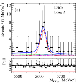
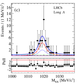
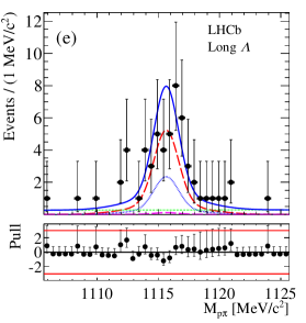
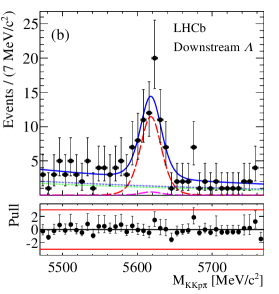
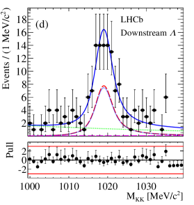
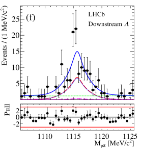
Figure 2: Fit projections to the ${{p}{{\pi}^{-}}{{K}^{+}}{{K}^{-}}}$invariant mass in the (a) long and (b) downstream datasets, the ${{{K}^{+}}{{K}^{-}}}$invariant mass in the (c) long and (d) downstream datasets, and the ${{p}{{\pi}^{-}}}$invariant mass in the (e) long and (f) downstream datasets. The total fit projection is given by the blue solid line. The blue and green dotted lines represent the $\phi$ + ${\mathchar 28931\relax}$ and pure combinatorial fit components, respectively. The red and magenta dashed lines represent the ${{{\mathchar 28931\relax}^{0}_{b}}\!\rightarrow{\mathchar 28931\relax}\phi}$ signal and the ${{\mathchar 28931\relax}^{0}_{b}}\rightarrow{\mathchar 28931\relax}{{K}^{+}}{{K}^{-}}$ non-resonant components, respectively. Black points represent the data. Data uncertainties are Poisson 68% confidence intervals.

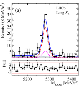
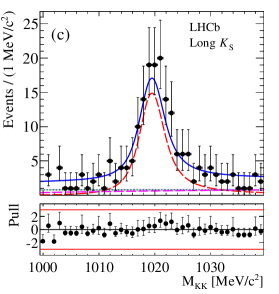
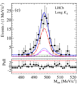
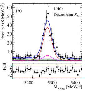
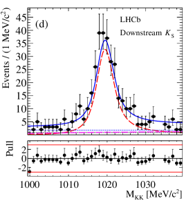
Figure 3: Fit projections to the ${{{\pi}^{+}}{{\pi}^{-}}{{K}^{+}}{{K}^{-}}}$invariant mass in the (a) long and (b) downstream datasets, the ${{{K}^{+}}{{K}^{-}}}$invariant mass in the (c) long and (d) downstream datasets, and the ${{{\pi}^{+}}{{\pi}^{-}}}$ invariant mass in the (e) long and (f) downstream datasets. The total fit projection is given by the blue solid line. The green and blue dotted lines represent the combinatorial and ${K}^{0}_{\mathrm{\scriptscriptstyle S}}$ + random ${K}^{+}$ ${K}^{-}$ fit components, respectively. The red and magenta dashed lines represent the ${{{B}^{0}}\!\rightarrow{{K}^{0}_{\mathrm{\scriptscriptstyle S}}}\phi}$ signal and the ${{B}^{0}}\rightarrow{{K}^{0}_{\mathrm{\scriptscriptstyle S}}}{{K}^{+}}{{K}^{-}}$ non-resonant components, respectively. Black points represent the data. Data uncertainties are Poisson 68% confidence intervals.

The yields of the ${{\mathchar 28931\relax}^{0}_{b}}\!\rightarrow{\mathchar 28931\relax}\phi$ signal and ${{B}^{0}}\!\rightarrow{{K}^{0}_{\mathrm{\scriptscriptstyle S}}}\phi$ control mode are determined from simultaneous extended unbinned maximum likelihood fits to the respective datasets divided according to the data-taking period and also according to whether the ${\mathchar 28931\relax}\,({{K}^{0}_{\mathrm{\scriptscriptstyle S}}})$ decay products are reconstructed as long or downstream tracks. Efficiencies are applied to each dataset individually. The projections of the fit result to ${{\mathchar 28931\relax}^{0}_{b}}\!\rightarrow{\mathchar 28931\relax}\phi$ data are shown in Fig. 2. The fitted yields are $350\pm 24$ and $89\pm 13$ for the ${{B}^{0}}\!\rightarrow{{K}^{0}_{\mathrm{\scriptscriptstyle S}}}\phi$ and ${{\mathchar 28931\relax}^{0}_{b}}\!\rightarrow{\mathchar 28931\relax}\phi$ decay modes, respectively. The statistical significance of the ${{\mathchar 28931\relax}^{0}_{b}}\!\rightarrow{\mathchar 28931\relax}\phi$ decay, determined according to Wilks’ theorem [37] from the difference in the likelihood value of the fits with and without the ${{\mathchar 28931\relax}^{0}_{b}}\!\rightarrow{\mathchar 28931\relax}\phi$ component, is found to be $6.5$ standard deviations. With the systematic uncertainties discussed below included, the significance of the observed ${{\mathchar 28931\relax}^{0}_{b}}\!\rightarrow{\mathchar 28931\relax}\phi$ decay yield is calculated to be $5.9$ standard deviations. The projections of the fit result to the ${{B}^{0}}\!\rightarrow{{K}^{0}_{\mathrm{\scriptscriptstyle S}}}\phi$ data are shown in Fig. 3. The fit is found to describe the data well in all three dimensions and a clear peak from the control mode is seen.

The systematic contributions to the branching fraction uncertainty budget are summarised in Table 1. The largest contributions to the systematic uncertainties result from data-driven corrections applied to simulated data along with the mass model used to determine the signal yields.

Table 1: Systematic uncertainty contributions to the branching fraction ratio.

Source	Uncertainty (%)
Mass model	3.0
Simulation sample size	2.2
Tracking efficiency	0.5
Vertex efficiency	2.6
Hardware trigger	2.8
Selection efficiency	4.1
Peaking background	0.1
Total	6.7

Signal mismodelling is accounted for using a one-dimensional kernel estimate for the description of the simulated mass distributions [38]. Background mismodelling is accounted for using a linear function. The kernel estimate is used in both the signal and control channels to describe the ${\mathchar 28931\relax}^{0}_{b}$, ${B}^{0}$, ${K}^{0}_{\mathrm{\scriptscriptstyle S}}$, and ${\mathchar 28931\relax}$ line shapes. In order to determine the systematic uncertainties, 1000 pseudoexperiments are generated with the alternative model and are subsequently fitted with the nominal model. The average difference between the generated and fitted yield values is taken as the systematic uncertainty. This leads to uncertainties of 3.0% and 0.6% for the signal and control mode yields, respectively.

Systematic uncertainties associated with the efficiency corrections from simulated datasets are considered. The limited size of the simulated sample gives rise to an uncertainty of 2.2%. The main uncertainties in the tracking and vertexing correction factors arise from the limited size of the control sample, which leads to uncertainties of 0.5% and 2.6%, respectively. For the case of the trigger efficiency, uncertainties related to the software trigger cancel between the signal and control modes, as the software trigger decision is made only on the decay products of the $\phi$ meson. Uncertainties in the efficiency of the hardware trigger selections are estimated using data-driven methods, for which an uncertainty of 2.8% is applied. The BDTs used to select signal and control modes use the same input variables. Biases could exist if the simulation mismodels these variables differently for signal and control modes. In order to quantify this effect, the control mode is selected with the same classifier as the signal decay. The difference in the measured branching fraction is found to be 4.1%.

The ${{\mathchar 28931\relax}^{0}_{b}}\rightarrow\mathchar 28934\relax^{0}(\rightarrow{\mathchar 28931\relax}\gamma){{K}^{+}}{{K}^{-}}$ and ${{\mathchar 28931\relax}^{0}_{b}}\rightarrow{p}{{K}^{-}}\phi$ decay modes are found to be the only significant peaking background contributions. However, for the case of the ${{\mathchar 28931\relax}^{0}_{b}}\rightarrow{p}{{K}^{-}}\phi$ decay, the resulting candidates are reconstructed in the long dataset only. With the assumption that the branching fraction for this decay is the same size as for the signal, the contribution is $<1\%$ compared to the ${{\mathchar 28931\relax}^{0}_{b}}\!\rightarrow{\mathchar 28931\relax}\phi$ decay and far from the ${\mathchar 28931\relax}^{0}_{b}$ signal region, and is therefore ignored. In order to determine the shape in the ${p}{{\pi}^{-}}{{K}^{+}}{{K}^{-}}$ spectrum of the ${{\mathchar 28931\relax}^{0}_{b}}\rightarrow\mathchar 28934\relax^{0}{{K}^{+}}{{K}^{-}}$ decay, a sample of ${{\mathchar 28931\relax}^{0}_{b}}\rightarrow\mathchar 28934\relax^{0}{{K}^{+}}{{K}^{-}}$ simulated events is used with a requirement that the ${{K}^{+}}{{K}^{-}}$ invariant mass is within 30${\mathrm{\,Me\kern-1.00006ptV\!/}c^{2}}$ of the nominal $\phi$ mass. The inclusion of an additional fit component using the shape from simulation is found to have a small effect on the signal yield at the level of 0.1%, which is assigned as a systematic uncertainty. For the case of the ${{{B}^{0}}\!\rightarrow{{K}^{0}_{\mathrm{\scriptscriptstyle S}}}\phi}$ control mode, no peaking background contributions have been identified.

The branching fraction ratio is measured to be

$$\frac{{\mathcal{B}}({{{\mathchar 28931\relax}^{0}_{b}}\!\rightarrow{\mathchar 28931\relax}\phi})}{{\mathcal{B}}({{{B}^{0}}\!\rightarrow{{K}^{0}_{\mathrm{\scriptscriptstyle S}}}\phi})}\frac{f_{{{\mathchar 28931\relax}^{0}_{b}}}}{f_{{{B}^{0}}}}=0.55\pm 0.11\mathrm{\,(stat)}\pm 0.04\mathrm{\,(syst)}.$$

The use of the world average value of ${\mathcal{B}}({{{B}^{0}}\!\rightarrow{{K}^{0}_{\mathrm{\scriptscriptstyle S}}}\phi})=(3.65\,^{+0.35}_{-0.30})\times 10^{-6}$ [15] gives the final result of

$${\mathcal{B}}({{{\mathchar 28931\relax}^{0}_{b}}\!\rightarrow{\mathchar 28931\relax}\phi})/10^{-6} =$$

$$5.18\pm 1.04\mathrm{\,(stat)}\pm 0.35\mathrm{\,(syst)}\,^{+0.50}_{-0.43}\,({\mathcal{B}}({{{B}^{0}}\!\rightarrow{{K}^{0}_{\mathrm{\scriptscriptstyle S}}}\phi}))\pm 0.44\,(f_{d}/f_{{{\mathchar 28931\relax}^{0}_{b}}}).$$

6 Triple-product asymmetries

The ${{\mathchar 28931\relax}^{0}_{b}}\!\rightarrow{\mathchar 28931\relax}\phi$ decay is a spin-$1/2$ to spin-$1/2$ plus vector transition. Five angles are needed to describe this decay since ${\mathchar 28931\relax}^{0}_{b}$ baryons may potentially be produced with a transverse polarisation in proton-proton collisions [13], as shown in Fig. 4. The angle $\theta$ is defined as the polar angle of the ${\mathchar 28931\relax}$ baryon in the ${\mathchar 28931\relax}^{0}_{b}$ rest frame with respect to the normal vector defined through

$$\hat{n}=\frac{\vec{p}_{1}\times\vec{p}_{{{\mathchar 28931\relax}^{0}_{b}}}}{|\vec{p}_{1}\times\vec{p}_{{{\mathchar 28931\relax}^{0}_{b}}}|},$$ (2)

where $\vec{p}_{1}$ is the momentum of an incoming proton and $\vec{p}_{{{\mathchar 28931\relax}^{0}_{b}}}$ is the momentum of the ${\mathchar 28931\relax}^{0}_{b}$ baryon. The angles $\theta_{\mathchar 28931\relax}$ and $\Phi_{\mathchar 28931\relax}$ are defined as the polar and azimuthal angles of the proton from the decay of the ${\mathchar 28931\relax}$ baryon in the ${\mathchar 28931\relax}$ rest frame. The angles $\theta_{\phi}$ and $\Phi_{\phi}$ are defined as the polar and azimuthal angles of the ${K}^{+}$ meson in the rest frame of the $\phi$ meson.

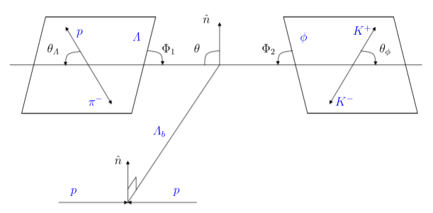
Figure 4: Decay angles for the ${{\mathchar 28931\relax}^{0}_{b}}\!\rightarrow{\mathchar 28931\relax}\phi$ decay, where the angles are defined in the text.

Triple-product asymmetries, which are odd under time-reversal, have been proposed by Leitner and Ajaltouni using the azimuthal angles $\Phi_{n_{i}},i\in\{{\mathchar 28931\relax},\phi\}$, defined as [12]

$$\cos\Phi_{n_{i}} =\vec{e}_{Y}\cdot\vec{u}_{i},$$ (3)

$$\sin\Phi_{n_{i}} =\vec{e}_{Z}\cdot(\vec{e}_{Y}\times\vec{u}_{i}),$$ (4)

where

$$\vec{u}_{i}=\frac{\vec{e}_{Z}\times\hat{n}_{i}}{|\vec{e}_{Z}\times\hat{n}_{i}|}.$$ (5)

The basis $\{\vec{e}_{X},\vec{e}_{Y},\vec{e}_{Z}\}$ is defined in the ${\mathchar 28931\relax}^{0}_{b}$ rest frame, in which $\vec{e}_{Z}$ is parallel to $\hat{n}$, $\vec{e}_{X}$ is chosen to be parallel to the momentum of the incoming proton, and $\hat{n}_{{\mathchar 28931\relax}(\phi)}$ is the normal vector to the ${\mathchar 28931\relax}(\phi)$ decay plane, defined through

$$\hat{n}_{\mathchar 28931\relax} =\frac{\vec{p}_{p}\times\vec{p}_{\pi}}{|\vec{p}_{p}\times\vec{p}_{\pi}|},$$ (6)

$$\hat{n}_{\phi} =\frac{\vec{p}_{{{K}^{+}}}\times\vec{p}_{{{K}^{-}}}}{|\vec{p}_{{{K}^{+}}}\times\vec{p}_{{{K}^{-}}}|}.$$ (7)

Asymmetries in $\cos\Phi_{n_{i}}$ and $\sin\Phi_{n_{i}}$, where $i\in\{{\mathchar 28931\relax},\phi\}$, are defined as

$$A_{i}^{c} =\frac{N^{+,c}_{i}-N^{-,c}_{i}}{N^{+,c}_{i}+N^{-,c}_{i}},$$ (8)

$$A_{i}^{s} =\frac{N^{+,s}_{i}-N^{-,s}_{i}}{N^{+,s}_{i}+N^{-,s}_{i}},$$ (9)

where $N^{+(-),c}_{i}$ and $N^{+(-),s}_{i}$ denote the number of candidates for which the $\cos\Phi_{n_{i}}$ and $\sin\Phi_{n_{i}}$ observables are positive (negative), respectively.

The asymmetries $A_{\mathchar 28931\relax}^{c,s}$ and $A_{\phi}^{c,s}$ are determined experimentally through a simultaneous unbinned maximum likelihood fit to datasets in which the relevant observables are positive and negative. The fit construction and observables are identical to that used for the branching fraction measurement. However, the yields for each dataset are parametrised in terms of the total yield, $N_{j}$, and the asymmetry, $A_{j}$, for fit component $j$ as

$$N^{+}_{j} =\frac{N^{j}}{2}(1+A_{j}),$$ (10)

$$N^{-}_{j} =\frac{N^{j}}{2}(1-A_{j}).$$ (11)

Distributions of the $\sin\Phi_{n_{({\mathchar 28931\relax},\phi)}}$ and $\cos\Phi_{n_{({\mathchar 28931\relax},\phi)}}$ observables from ${{\mathchar 28931\relax}^{0}_{b}}\!\rightarrow{\mathchar 28931\relax}\phi$ data have been extracted using the sPlot method [39] and are provided in Fig. 5. The numerical values of the fitted asymmetries are given in Table 2.

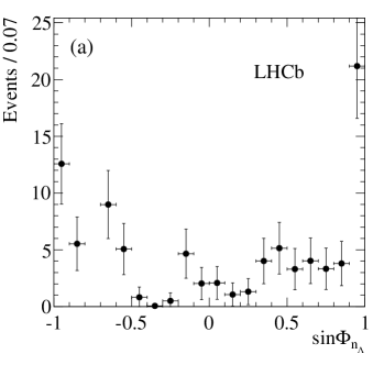
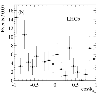
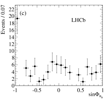
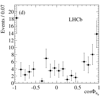
Figure 5: Distributions of the angular observables: (a) $\sin\Phi_{n_{\mathchar 28931\relax}}$, (b) $\cos\Phi_{n_{\mathchar 28931\relax}}$, (c) $\sin\Phi_{n_{\phi}}$, (d) $\cos\Phi_{n_{\phi}}$ from weighted ${{\mathchar 28931\relax}^{0}_{b}}\!\rightarrow{\mathchar 28931\relax}\phi$ data.

Table 2: Asymmetries measured from ${{\mathchar 28931\relax}^{0}_{b}}\!\rightarrow{\mathchar 28931\relax}\phi$ data events.

Asymmetry	Fit value
$A^{c}_{\mathchar 28931\relax}$	$-0.22\pm 0.12$
$A^{s}_{\mathchar 28931\relax}$	$0.13\pm 0.12$
$A^{c}_{\phi}$	$-0.01\pm 0.12$
$A^{s}_{\phi}$	$-0.07\pm 0.12$

Mismodelling of the mass components could lead to background contamination in the determination of the asymmetries. In the determination of the uncertainty related to the mass model, two contributions are considered. These are the line shape models and the background asymmetries. The effects of the line shapes are quantified using the same method as the branching fraction measurement, i.e. the generation of datasets with a one-dimensional kernel estimate of the simulation mass distributions in addition to modification of the background description. In the nominal fit, components that are not from the ${{\mathchar 28931\relax}^{0}_{b}}\!\rightarrow{\mathchar 28931\relax}\phi$ signal have zero asymmetries. For background components this is justified due to the uncorrelated kinematics of the ${K}^{+}$ ${K}^{-}$ and $p$ ${\pi}^{-}$ systems. However, the non-resonant ${{\mathchar 28931\relax}^{0}_{b}}\rightarrow{\mathchar 28931\relax}{{K}^{+}}{{K}^{-}}$ contribution could have non-zero asymmetries. The systematic uncertainty due to the assumption of zero background asymmetries is determined through comparing the nominal fit against the fit with all possible asymmetries allowed to vary freely.

Efficiencies are found to be independent of the $\sin\Phi_{n_{i}}$ and $\cos\Phi_{n_{i}}$ observables. The systematic uncertainty due to the angular acceptance is then taken from the statistical uncertainty in fits to the simulated datasets, after the application of an appropriate weighting to account for the differences between data and simulation. The resolutions of the angular observables are found from simulated events to be 32.3$\mathrm{\,mrad}$ and 22.1$\mathrm{\,mrad}$ for the $\Phi_{n_{\mathchar 28931\relax}}$ and $\Phi_{n_{\phi}}$ angles, respectively. The uncertainty due to bin migration is then assigned assuming maximal asymmetry and leads to minor uncertainties of 0.007 for the $\Phi_{n_{\phi}}$ angle and 0.010 for the $\Phi_{n_{\mathchar 28931\relax}}$ angle. Systematic contributions to the triple-product uncertainty budget are summarised in Table 3.

Table 3: Systematic uncertainty contributions to the triple-product asymmetries.

Source	$A_{\mathchar 28931\relax}^{c}$	$A_{\mathchar 28931\relax}^{s}$	$A_{\phi}^{c}$	$A_{\phi}^{s}$
Mass model	0.061	0.051	0.026	0.009
Angular acceptance	0.010	0.010	0.010	0.010
Angular resolution	0.008	0.008	0.005	0.005
Total	0.062	0.053	0.028	0.014

7 Summary

A search for the ${{\mathchar 28931\relax}^{0}_{b}}\rightarrow{\mathchar 28931\relax}\phi$ decay is presented based on a dataset of 3.0$\mbox{\,fb}^{-1}$ collected by the LHCb experiment in 2011 and 2012. The decay is observed for the first time with a significance of $5.9$ standard deviations including systematic uncertainties. The branching fraction is found to be

$${\mathcal{B}}({{{\mathchar 28931\relax}^{0}_{b}}\!\rightarrow{\mathchar 28931\relax}\phi})/10^{-6} =$$

$$5.18\pm 1.04\mathrm{\,(stat)}\pm 0.35\mathrm{\,(syst)}\,^{+0.50}_{-0.43}\,({\mathcal{B}}({{{B}^{0}}\!\rightarrow{{K}^{0}_{\mathrm{\scriptscriptstyle S}}}\phi}))\pm 0.44\,(f_{d}/f_{{{\mathchar 28931\relax}^{0}_{b}}}).$$

Triple-product asymmetries are measured to be

$$A^{c}_{\mathchar 28931\relax} =-0.22\pm 0.12\mathrm{\,(stat)}\pm 0.06\mathrm{\,(syst)},$$

$$A^{s}_{\mathchar 28931\relax} =\phantom{-}0.13\pm 0.12\mathrm{\,(stat)}\pm 0.05\mathrm{\,(syst)},$$

$$A^{c}_{\phi} =-0.01\pm 0.12\mathrm{\,(stat)}\pm 0.03\mathrm{\,(syst)},$$

$$A^{s}_{\phi} =-0.07\pm 0.12\mathrm{\,(stat)}\pm 0.01\mathrm{\,(syst)},$$

and are consistent with zero. Data collected by the LHCb experiment in the forthcoming years will improve the statistical precision of these measurements and enable the dynamics of ${b}\rightarrow{s}$ transitions in beauty baryons to be probed in greater detail, which will greatly enhance the reach of searches for physics beyond the SM.

LHCb collaboration

R. Aaij³⁹, C. Abellán Beteta⁴¹, B. Adeva³⁸, M. Adinolfi⁴⁷, Z. Ajaltouni⁵, S. Akar⁶, J. Albrecht¹⁰, F. Alessio³⁹, M. Alexander⁵², S. Ali⁴², G. Alkhazov³¹, P. Alvarez Cartelle⁵⁴, A.A. Alves Jr⁵⁸, S. Amato², S. Amerio²³, Y. Amhis⁷, L. An^3,40, L. Anderlini¹⁸, G. Andreassi⁴⁰, M. Andreotti^17,g, J.E. Andrews⁵⁹, R.B. Appleby⁵⁵, O. Aquines Gutierrez¹¹, F. Archilli³⁹, P. d’Argent¹², A. Artamonov³⁶, M. Artuso⁶⁰, E. Aslanides⁶, G. Auriemma^26,n, M. Baalouch⁵, S. Bachmann¹², J.J. Back⁴⁹, A. Badalov³⁷, C. Baesso⁶¹, S. Baker⁵⁴, W. Baldini¹⁷, R.J. Barlow⁵⁵, C. Barschel³⁹, S. Barsuk⁷, W. Barter³⁹, V. Batozskaya²⁹, V. Battista⁴⁰, A. Bay⁴⁰, L. Beaucourt⁴, J. Beddow⁵², F. Bedeschi²⁴, I. Bediaga¹, L.J. Bel⁴², V. Bellee⁴⁰, N. Belloli^21,k, I. Belyaev³², E. Ben-Haim⁸, G. Bencivenni¹⁹, S. Benson³⁹, J. Benton⁴⁷, A. Berezhnoy³³, R. Bernet⁴¹, A. Bertolin²³, F. Betti¹⁵, M.-O. Bettler³⁹, M. van Beuzekom⁴², S. Bifani⁴⁶, P. Billoir⁸, T. Bird⁵⁵, A. Birnkraut¹⁰, A. Bizzeti^18,i, T. Blake⁴⁹, F. Blanc⁴⁰, J. Blouw¹¹, S. Blusk⁶⁰, V. Bocci²⁶, A. Bondar³⁵, N. Bondar^31,39, W. Bonivento¹⁶, A. Borgheresi^21,k, S. Borghi⁵⁵, M. Borisyak⁶⁷, M. Borsato³⁸, M. Boubdir⁹, T.J.V. Bowcock⁵³, E. Bowen⁴¹, C. Bozzi^17,39, S. Braun¹², M. Britsch¹², T. Britton⁶⁰, J. Brodzicka⁵⁵, E. Buchanan⁴⁷, C. Burr⁵⁵, A. Bursche², J. Buytaert³⁹, S. Cadeddu¹⁶, R. Calabrese^17,g, M. Calvi^21,k, M. Calvo Gomez^37,p, P. Campana¹⁹, D. Campora Perez³⁹, L. Capriotti⁵⁵, A. Carbone^15,e, G. Carboni^25,l, R. Cardinale^20,j, A. Cardini¹⁶, P. Carniti^21,k, L. Carson⁵¹, K. Carvalho Akiba², G. Casse⁵³, L. Cassina^21,k, L. Castillo Garcia⁴⁰, M. Cattaneo³⁹, Ch. Cauet¹⁰, G. Cavallero²⁰, R. Cenci^24,t, M. Charles⁸, Ph. Charpentier³⁹, G. Chatzikonstantinidis⁴⁶, M. Chefdeville⁴, S. Chen⁵⁵, S.-F. Cheung⁵⁶, M. Chrzaszcz^41,27, X. Cid Vidal³⁹, G. Ciezarek⁴², P.E.L. Clarke⁵¹, M. Clemencic³⁹, H.V. Cliff⁴⁸, J. Closier³⁹, V. Coco⁵⁸, J. Cogan⁶, E. Cogneras⁵, V. Cogoni^16,f, L. Cojocariu³⁰, G. Collazuol^23,r, P. Collins³⁹, A. Comerma-Montells¹², A. Contu³⁹, A. Cook⁴⁷, M. Coombes⁴⁷, S. Coquereau⁸, G. Corti³⁹, M. Corvo^17,g, B. Couturier³⁹, G.A. Cowan⁵¹, D.C. Craik⁵¹, A. Crocombe⁴⁹, M. Cruz Torres⁶¹, S. Cunliffe⁵⁴, R. Currie⁵⁴, C. D’Ambrosio³⁹, E. Dall’Occo⁴², J. Dalseno⁴⁷, P.N.Y. David⁴², A. Davis⁵⁸, O. De Aguiar Francisco², K. De Bruyn⁶, S. De Capua⁵⁵, M. De Cian¹², J.M. De Miranda¹, L. De Paula², P. De Simone¹⁹, C.-T. Dean⁵², D. Decamp⁴, M. Deckenhoff¹⁰, L. Del Buono⁸, N. Déléage⁴, M. Demmer¹⁰, D. Derkach⁶⁷, O. Deschamps⁵, F. Dettori³⁹, B. Dey²², A. Di Canto³⁹, F. Di Ruscio²⁵, H. Dijkstra³⁹, F. Dordei³⁹, M. Dorigo⁴⁰, A. Dosil Suárez³⁸, A. Dovbnya⁴⁴, K. Dreimanis⁵³, L. Dufour⁴², G. Dujany⁵⁵, K. Dungs³⁹, P. Durante³⁹, R. Dzhelyadin³⁶, A. Dziurda²⁷, A. Dzyuba³¹, S. Easo^50,39, U. Egede⁵⁴, V. Egorychev³², S. Eidelman³⁵, S. Eisenhardt⁵¹, U. Eitschberger¹⁰, R. Ekelhof¹⁰, L. Eklund⁵², I. El Rifai⁵, Ch. Elsasser⁴¹, S. Ely⁶⁰, S. Esen¹², H.M. Evans⁴⁸, T. Evans⁵⁶, A. Falabella¹⁵, C. Färber³⁹, N. Farley⁴⁶, S. Farry⁵³, R. Fay⁵³, D. Fazzini^21,k, D. Ferguson⁵¹, V. Fernandez Albor³⁸, F. Ferrari¹⁵, F. Ferreira Rodrigues¹, M. Ferro-Luzzi³⁹, S. Filippov³⁴, M. Fiore^17,g, M. Fiorini^17,g, M. Firlej²⁸, C. Fitzpatrick⁴⁰, T. Fiutowski²⁸, F. Fleuret^7,b, K. Fohl³⁹, M. Fontana¹⁶, F. Fontanelli^20,j, D. C. Forshaw⁶⁰, R. Forty³⁹, M. Frank³⁹, C. Frei³⁹, M. Frosini¹⁸, J. Fu²², E. Furfaro^25,l, A. Gallas Torreira³⁸, D. Galli^15,e, S. Gallorini²³, S. Gambetta⁵¹, M. Gandelman², P. Gandini⁵⁶, Y. Gao³, J. García Pardiñas³⁸, J. Garra Tico⁴⁸, L. Garrido³⁷, P.J. Garsed⁴⁸, D. Gascon³⁷, C. Gaspar³⁹, L. Gavardi¹⁰, G. Gazzoni⁵, D. Gerick¹², E. Gersabeck¹², M. Gersabeck⁵⁵, T. Gershon⁴⁹, Ph. Ghez⁴, S. Gianì⁴⁰, V. Gibson⁴⁸, O.G. Girard⁴⁰, L. Giubega³⁰, V.V. Gligorov³⁹, C. Göbel⁶¹, D. Golubkov³², A. Golutvin^54,39, A. Gomes^1,a, C. Gotti^21,k, M. Grabalosa Gándara⁵, R. Graciani Diaz³⁷, L.A. Granado Cardoso³⁹, E. Graugés³⁷, E. Graverini⁴¹, G. Graziani¹⁸, A. Grecu³⁰, P. Griffith⁴⁶, L. Grillo¹², O. Grünberg⁶⁵, B. Gui⁶⁰, E. Gushchin³⁴, Yu. Guz^36,39, T. Gys³⁹, T. Hadavizadeh⁵⁶, C. Hadjivasiliou⁶⁰, G. Haefeli⁴⁰, C. Haen³⁹, S.C. Haines⁴⁸, S. Hall⁵⁴, B. Hamilton⁵⁹, X. Han¹², S. Hansmann-Menzemer¹², N. Harnew⁵⁶, S.T. Harnew⁴⁷, J. Harrison⁵⁵, J. He³⁹, T. Head⁴⁰, A. Heister⁹, K. Hennessy⁵³, P. Henrard⁵, L. Henry⁸, J.A. Hernando Morata³⁸, E. van Herwijnen³⁹, M. Heß⁶⁵, A. Hicheur², D. Hill⁵⁶, M. Hoballah⁵, C. Hombach⁵⁵, L. Hongming⁴⁰, W. Hulsbergen⁴², T. Humair⁵⁴, M. Hushchyn⁶⁷, N. Hussain⁵⁶, D. Hutchcroft⁵³, M. Idzik²⁸, P. Ilten⁵⁷, R. Jacobsson³⁹, A. Jaeger¹², J. Jalocha⁵⁶, E. Jans⁴², A. Jawahery⁵⁹, M. John⁵⁶, D. Johnson³⁹, C.R. Jones⁴⁸, C. Joram³⁹, B. Jost³⁹, N. Jurik⁶⁰, S. Kandybei⁴⁴, W. Kanso⁶, M. Karacson³⁹, T.M. Karbach^39,†, S. Karodia⁵², M. Kecke¹², M. Kelsey⁶⁰, I.R. Kenyon⁴⁶, M. Kenzie³⁹, T. Ketel⁴³, E. Khairullin⁶⁷, B. Khanji^21,39,k, C. Khurewathanakul⁴⁰, T. Kirn⁹, S. Klaver⁵⁵, K. Klimaszewski²⁹, M. Kolpin¹², I. Komarov⁴⁰, R.F. Koopman⁴³, P. Koppenburg^42,39, M. Kozeiha⁵, L. Kravchuk³⁴, K. Kreplin¹², M. Kreps⁴⁹, P. Krokovny³⁵, F. Kruse¹⁰, W. Krzemien²⁹, W. Kucewicz^27,o, M. Kucharczyk²⁷, V. Kudryavtsev³⁵, A. K. Kuonen⁴⁰, K. Kurek²⁹, T. Kvaratskheliya³², D. Lacarrere³⁹, G. Lafferty^55,39, A. Lai¹⁶, D. Lambert⁵¹, G. Lanfranchi¹⁹, C. Langenbruch⁴⁹, B. Langhans³⁹, T. Latham⁴⁹, C. Lazzeroni⁴⁶, R. Le Gac⁶, J. van Leerdam⁴², J.-P. Lees⁴, R. Lefèvre⁵, A. Leflat^33,39, J. Lefrançois⁷, E. Lemos Cid³⁸, O. Leroy⁶, T. Lesiak²⁷, B. Leverington¹², Y. Li⁷, T. Likhomanenko^67,66, R. Lindner³⁹, C. Linn³⁹, F. Lionetto⁴¹, B. Liu¹⁶, X. Liu³, D. Loh⁴⁹, I. Longstaff⁵², J.H. Lopes², D. Lucchesi^23,r, M. Lucio Martinez³⁸, H. Luo⁵¹, A. Lupato²³, E. Luppi^17,g, O. Lupton⁵⁶, N. Lusardi²², A. Lusiani²⁴, X. Lyu⁶², F. Machefert⁷, F. Maciuc³⁰, O. Maev³¹, K. Maguire⁵⁵, S. Malde⁵⁶, A. Malinin⁶⁶, G. Manca⁷, G. Mancinelli⁶, P. Manning⁶⁰, A. Mapelli³⁹, J. Maratas⁵, J.F. Marchand⁴, U. Marconi¹⁵, C. Marin Benito³⁷, P. Marino^24,t, J. Marks¹², G. Martellotti²⁶, M. Martin⁶, M. Martinelli⁴⁰, D. Martinez Santos³⁸, F. Martinez Vidal⁶⁸, D. Martins Tostes², L.M. Massacrier⁷, A. Massafferri¹, R. Matev³⁹, A. Mathad⁴⁹, Z. Mathe³⁹, C. Matteuzzi²¹, A. Mauri⁴¹, B. Maurin⁴⁰, A. Mazurov⁴⁶, M. McCann⁵⁴, J. McCarthy⁴⁶, A. McNab⁵⁵, R. McNulty¹³, B. Meadows⁵⁸, F. Meier¹⁰, M. Meissner¹², D. Melnychuk²⁹, M. Merk⁴², A Merli^22,u, E Michielin²³, D.A. Milanes⁶⁴, M.-N. Minard⁴, D.S. Mitzel¹², J. Molina Rodriguez⁶¹, I.A. Monroy⁶⁴, S. Monteil⁵, M. Morandin²³, P. Morawski²⁸, A. Mordà⁶, M.J. Morello^24,t, J. Moron²⁸, A.B. Morris⁵¹, R. Mountain⁶⁰, F. Muheim⁵¹, D. Müller⁵⁵, J. Müller¹⁰, K. Müller⁴¹, V. Müller¹⁰, M. Mussini¹⁵, B. Muster⁴⁰, P. Naik⁴⁷, T. Nakada⁴⁰, R. Nandakumar⁵⁰, A. Nandi⁵⁶, I. Nasteva², M. Needham⁵¹, N. Neri²², S. Neubert¹², N. Neufeld³⁹, M. Neuner¹², A.D. Nguyen⁴⁰, C. Nguyen-Mau^40,q, V. Niess⁵, S. Nieswand⁹, R. Niet¹⁰, N. Nikitin³³, T. Nikodem¹², A. Novoselov³⁶, D.P. O’Hanlon⁴⁹, A. Oblakowska-Mucha²⁸, V. Obraztsov³⁶, S. Ogilvy⁵², O. Okhrimenko⁴⁵, R. Oldeman^16,48,f, C.J.G. Onderwater⁶⁹, B. Osorio Rodrigues¹, J.M. Otalora Goicochea², A. Otto³⁹, P. Owen⁵⁴, A. Oyanguren⁶⁸, A. Palano^14,d, F. Palombo^22,u, M. Palutan¹⁹, J. Panman³⁹, A. Papanestis⁵⁰, M. Pappagallo⁵², L.L. Pappalardo^17,g, C. Pappenheimer⁵⁸, W. Parker⁵⁹, C. Parkes⁵⁵, G. Passaleva¹⁸, G.D. Patel⁵³, M. Patel⁵⁴, C. Patrignani^20,j, A. Pearce^55,50, A. Pellegrino⁴², G. Penso^26,m, M. Pepe Altarelli³⁹, S. Perazzini^15,e, P. Perret⁵, L. Pescatore⁴⁶, K. Petridis⁴⁷, A. Petrolini^20,j, M. Petruzzo²², E. Picatoste Olloqui³⁷, B. Pietrzyk⁴, M. Pikies²⁷, D. Pinci²⁶, A. Pistone²⁰, A. Piucci¹², S. Playfer⁵¹, M. Plo Casasus³⁸, T. Poikela³⁹, F. Polci⁸, A. Poluektov^49,35, I. Polyakov³², E. Polycarpo², A. Popov³⁶, D. Popov^11,39, B. Popovici³⁰, C. Potterat², E. Price⁴⁷, J.D. Price⁵³, J. Prisciandaro³⁸, A. Pritchard⁵³, C. Prouve⁴⁷, V. Pugatch⁴⁵, A. Puig Navarro⁴⁰, G. Punzi^24,s, W. Qian⁵⁶, R. Quagliani^7,47, B. Rachwal²⁷, J.H. Rademacker⁴⁷, M. Rama²⁴, M. Ramos Pernas³⁸, M.S. Rangel², I. Raniuk⁴⁴, G. Raven⁴³, F. Redi⁵⁴, S. Reichert⁵⁵, A.C. dos Reis¹, V. Renaudin⁷, S. Ricciardi⁵⁰, S. Richards⁴⁷, M. Rihl³⁹, K. Rinnert^53,39, V. Rives Molina³⁷, P. Robbe⁷, A.B. Rodrigues¹, E. Rodrigues⁵⁵, J.A. Rodriguez Lopez⁶⁴, P. Rodriguez Perez⁵⁵, A. Rogozhnikov⁶⁷, S. Roiser³⁹, V. Romanovsky³⁶, A. Romero Vidal³⁸, J. W. Ronayne¹³, M. Rotondo²³, T. Ruf³⁹, P. Ruiz Valls⁶⁸, J.J. Saborido Silva³⁸, N. Sagidova³¹, B. Saitta^16,f, V. Salustino Guimaraes², C. Sanchez Mayordomo⁶⁸, B. Sanmartin Sedes³⁸, R. Santacesaria²⁶, C. Santamarina Rios³⁸, M. Santimaria¹⁹, E. Santovetti^25,l, A. Sarti^19,m, C. Satriano^26,n, A. Satta²⁵, D.M. Saunders⁴⁷, D. Savrina^32,33, S. Schael⁹, M. Schiller³⁹, H. Schindler³⁹, M. Schlupp¹⁰, M. Schmelling¹¹, T. Schmelzer¹⁰, B. Schmidt³⁹, O. Schneider⁴⁰, A. Schopper³⁹, M. Schubiger⁴⁰, M.-H. Schune⁷, R. Schwemmer³⁹, B. Sciascia¹⁹, A. Sciubba^26,m, A. Semennikov³², A. Sergi⁴⁶, N. Serra⁴¹, J. Serrano⁶, L. Sestini²³, P. Seyfert²¹, M. Shapkin³⁶, I. Shapoval^17,44,g, Y. Shcheglov³¹, T. Shears⁵³, L. Shekhtman³⁵, V. Shevchenko⁶⁶, A. Shires¹⁰, B.G. Siddi¹⁷, R. Silva Coutinho⁴¹, L. Silva de Oliveira², G. Simi^23,s, M. Sirendi⁴⁸, N. Skidmore⁴⁷, T. Skwarnicki⁶⁰, E. Smith⁵⁴, I.T. Smith⁵¹, J. Smith⁴⁸, M. Smith⁵⁵, H. Snoek⁴², M.D. Sokoloff⁵⁸, F.J.P. Soler⁵², F. Soomro⁴⁰, D. Souza⁴⁷, B. Souza De Paula², B. Spaan¹⁰, P. Spradlin⁵², S. Sridharan³⁹, F. Stagni³⁹, M. Stahl¹², S. Stahl³⁹, S. Stefkova⁵⁴, O. Steinkamp⁴¹, O. Stenyakin³⁶, S. Stevenson⁵⁶, S. Stoica³⁰, S. Stone⁶⁰, B. Storaci⁴¹, S. Stracka^24,t, M. Straticiuc³⁰, U. Straumann⁴¹, L. Sun⁵⁸, W. Sutcliffe⁵⁴, K. Swientek²⁸, S. Swientek¹⁰, V. Syropoulos⁴³, M. Szczekowski²⁹, T. Szumlak²⁸, S. T’Jampens⁴, A. Tayduganov⁶, T. Tekampe¹⁰, G. Tellarini^17,g, F. Teubert³⁹, C. Thomas⁵⁶, E. Thomas³⁹, J. van Tilburg⁴², V. Tisserand⁴, M. Tobin⁴⁰, S. Tolk⁴³, L. Tomassetti^17,g, D. Tonelli³⁹, S. Topp-Joergensen⁵⁶, E. Tournefier⁴, S. Tourneur⁴⁰, K. Trabelsi⁴⁰, M. Traill⁵², M.T. Tran⁴⁰, M. Tresch⁴¹, A. Trisovic³⁹, A. Tsaregorodtsev⁶, P. Tsopelas⁴², N. Tuning^42,39, A. Ukleja²⁹, A. Ustyuzhanin^67,66, U. Uwer¹², C. Vacca^16,39,f, V. Vagnoni¹⁵, S. Valat³⁹, G. Valenti¹⁵, A. Vallier⁷, R. Vazquez Gomez¹⁹, P. Vazquez Regueiro³⁸, C. Vázquez Sierra³⁸, S. Vecchi¹⁷, M. van Veghel⁴², J.J. Velthuis⁴⁷, M. Veltri^18,h, G. Veneziano⁴⁰, M. Vesterinen¹², B. Viaud⁷, D. Vieira², M. Vieites Diaz³⁸, X. Vilasis-Cardona^37,p, V. Volkov³³, A. Vollhardt⁴¹, D. Voong⁴⁷, A. Vorobyev³¹, V. Vorobyev³⁵, C. Voß⁶⁵, J.A. de Vries⁴², R. Waldi⁶⁵, C. Wallace⁴⁹, R. Wallace¹³, J. Walsh²⁴, J. Wang⁶⁰, D.R. Ward⁴⁸, N.K. Watson⁴⁶, D. Websdale⁵⁴, A. Weiden⁴¹, M. Whitehead³⁹, J. Wicht⁴⁹, G. Wilkinson^56,39, M. Wilkinson⁶⁰, M. Williams³⁹, M.P. Williams⁴⁶, M. Williams⁵⁷, T. Williams⁴⁶, F.F. Wilson⁵⁰, J. Wimberley⁵⁹, J. Wishahi¹⁰, W. Wislicki²⁹, M. Witek²⁷, G. Wormser⁷, S.A. Wotton⁴⁸, K. Wraight⁵², S. Wright⁴⁸, K. Wyllie³⁹, Y. Xie⁶³, Z. Xu⁴⁰, Z. Yang³, H. Yin⁶³, J. Yu⁶³, X. Yuan³⁵, O. Yushchenko³⁶, M. Zangoli¹⁵, M. Zavertyaev^11,c, L. Zhang³, Y. Zhang³, A. Zhelezov¹², Y. Zheng⁶², A. Zhokhov³², L. Zhong³, V. Zhukov⁹, S. Zucchelli¹⁵.

¹Centro Brasileiro de Pesquisas Físicas (CBPF), Rio de Janeiro, Brazil
²Universidade Federal do Rio de Janeiro (UFRJ), Rio de Janeiro, Brazil
³Center for High Energy Physics, Tsinghua University, Beijing, China
⁴LAPP, Université Savoie Mont-Blanc, CNRS/IN2P3, Annecy-Le-Vieux, France
⁵Clermont Université, Université Blaise Pascal, CNRS/IN2P3, LPC, Clermont-Ferrand, France
⁶CPPM, Aix-Marseille Université, CNRS/IN2P3, Marseille, France
⁷LAL, Université Paris-Sud, CNRS/IN2P3, Orsay, France
⁸LPNHE, Université Pierre et Marie Curie, Université Paris Diderot, CNRS/IN2P3, Paris, France
⁹I. Physikalisches Institut, RWTH Aachen University, Aachen, Germany
¹⁰Fakultät Physik, Technische Universität Dortmund, Dortmund, Germany
¹¹Max-Planck-Institut für Kernphysik (MPIK), Heidelberg, Germany
¹²Physikalisches Institut, Ruprecht-Karls-Universität Heidelberg, Heidelberg, Germany
¹³School of Physics, University College Dublin, Dublin, Ireland
¹⁴Sezione INFN di Bari, Bari, Italy
¹⁵Sezione INFN di Bologna, Bologna, Italy
¹⁶Sezione INFN di Cagliari, Cagliari, Italy
¹⁷Sezione INFN di Ferrara, Ferrara, Italy
¹⁸Sezione INFN di Firenze, Firenze, Italy
¹⁹Laboratori Nazionali dell’INFN di Frascati, Frascati, Italy
²⁰Sezione INFN di Genova, Genova, Italy
²¹Sezione INFN di Milano Bicocca, Milano, Italy
²²Sezione INFN di Milano, Milano, Italy
²³Sezione INFN di Padova, Padova, Italy
²⁴Sezione INFN di Pisa, Pisa, Italy
²⁵Sezione INFN di Roma Tor Vergata, Roma, Italy
²⁶Sezione INFN di Roma La Sapienza, Roma, Italy
²⁷Henryk Niewodniczanski Institute of Nuclear Physics Polish Academy of Sciences, Kraków, Poland
²⁸AGH - University of Science and Technology, Faculty of Physics and Applied Computer Science, Kraków, Poland
²⁹National Center for Nuclear Research (NCBJ), Warsaw, Poland
³⁰Horia Hulubei National Institute of Physics and Nuclear Engineering, Bucharest-Magurele, Romania
³¹Petersburg Nuclear Physics Institute (PNPI), Gatchina, Russia
³²Institute of Theoretical and Experimental Physics (ITEP), Moscow, Russia
³³Institute of Nuclear Physics, Moscow State University (SINP MSU), Moscow, Russia
³⁴Institute for Nuclear Research of the Russian Academy of Sciences (INR RAN), Moscow, Russia
³⁵Budker Institute of Nuclear Physics (SB RAS) and Novosibirsk State University, Novosibirsk, Russia
³⁶Institute for High Energy Physics (IHEP), Protvino, Russia
³⁷Universitat de Barcelona, Barcelona, Spain
³⁸Universidad de Santiago de Compostela, Santiago de Compostela, Spain
³⁹European Organization for Nuclear Research (CERN), Geneva, Switzerland
⁴⁰Ecole Polytechnique Fédérale de Lausanne (EPFL), Lausanne, Switzerland
⁴¹Physik-Institut, Universität Zürich, Zürich, Switzerland
⁴²Nikhef National Institute for Subatomic Physics, Amsterdam, The Netherlands
⁴³Nikhef National Institute for Subatomic Physics and VU University Amsterdam, Amsterdam, The Netherlands
⁴⁴NSC Kharkiv Institute of Physics and Technology (NSC KIPT), Kharkiv, Ukraine
⁴⁵Institute for Nuclear Research of the National Academy of Sciences (KINR), Kyiv, Ukraine
⁴⁶University of Birmingham, Birmingham, United Kingdom
⁴⁷H.H. Wills Physics Laboratory, University of Bristol, Bristol, United Kingdom
⁴⁸Cavendish Laboratory, University of Cambridge, Cambridge, United Kingdom
⁴⁹Department of Physics, University of Warwick, Coventry, United Kingdom
⁵⁰STFC Rutherford Appleton Laboratory, Didcot, United Kingdom
⁵¹School of Physics and Astronomy, University of Edinburgh, Edinburgh, United Kingdom
⁵²School of Physics and Astronomy, University of Glasgow, Glasgow, United Kingdom
⁵³Oliver Lodge Laboratory, University of Liverpool, Liverpool, United Kingdom
⁵⁴Imperial College London, London, United Kingdom
⁵⁵School of Physics and Astronomy, University of Manchester, Manchester, United Kingdom
⁵⁶Department of Physics, University of Oxford, Oxford, United Kingdom
⁵⁷Massachusetts Institute of Technology, Cambridge, MA, United States
⁵⁸University of Cincinnati, Cincinnati, OH, United States
⁵⁹University of Maryland, College Park, MD, United States
⁶⁰Syracuse University, Syracuse, NY, United States
⁶¹Pontifícia Universidade Católica do Rio de Janeiro (PUC-Rio), Rio de Janeiro, Brazil, associated to ^2
62University of Chinese Academy of Sciences, Beijing, China, associated to ^3
63Institute of Particle Physics, Central China Normal University, Wuhan, Hubei, China, associated to ^3
64Departamento de Fisica , Universidad Nacional de Colombia, Bogota, Colombia, associated to ^8
65Institut für Physik, Universität Rostock, Rostock, Germany, associated to ^12
66National Research Centre Kurchatov Institute, Moscow, Russia, associated to ^32
67Yandex School of Data Analysis, Moscow, Russia, associated to ^32
68Instituto de Fisica Corpuscular (IFIC), Universitat de Valencia-CSIC, Valencia, Spain, associated to ^37
69Van Swinderen Institute, University of Groningen, Groningen, The Netherlands, associated to <sup>42

a</sup>Universidade Federal do Triângulo Mineiro (UFTM), Uberaba-MG, Brazil
^bLaboratoire Leprince-Ringuet, Palaiseau, France
^cP.N. Lebedev Physical Institute, Russian Academy of Science (LPI RAS), Moscow, Russia
^dUniversità di Bari, Bari, Italy
^eUniversità di Bologna, Bologna, Italy
^fUniversità di Cagliari, Cagliari, Italy
^gUniversità di Ferrara, Ferrara, Italy
^hUniversità di Urbino, Urbino, Italy
ⁱUniversità di Modena e Reggio Emilia, Modena, Italy
^jUniversità di Genova, Genova, Italy
^kUniversità di Milano Bicocca, Milano, Italy
^lUniversità di Roma Tor Vergata, Roma, Italy
^mUniversità di Roma La Sapienza, Roma, Italy
ⁿUniversità della Basilicata, Potenza, Italy
^oAGH - University of Science and Technology, Faculty of Computer Science, Electronics and Telecommunications, Kraków, Poland
^pLIFAELS, La Salle, Universitat Ramon Llull, Barcelona, Spain
^qHanoi University of Science, Hanoi, Viet Nam
^rUniversità di Padova, Padova, Italy
^sUniversità di Pisa, Pisa, Italy
^tScuola Normale Superiore, Pisa, Italy
^uUniversità degli Studi di Milano, Milano, Italy
^†Deceased

References

- [1] Y. Shimizu, M. Tanimoto, and K. Yamamoto, Supersymmetry contributions to CP violations in and transitions taking account of new data, Phys. Rev. D87 (2013) 056004, arXiv:1212.6486
- [2] A. Datta, M. Imbeault, and D. London, , and new physics, Phys. Lett. B671 (2009) 256, arXiv:0811.2957
- [3] T. Moroi, CP violation in in SUSY GUT with right-handed neutrinos, Phys. Lett. B493 (2000) 366, arXiv:hep-ph/0007328
- [4] LHCb collaboration, R. Aaij et al., Measurement of violation in decays, Phys. Rev. D90 (2014) 052011, arXiv:1407.2222
- [5] LHCb collaboration, R. Aaij et al., First measurement of the -violating phase in decays, Phys. Rev. Lett. 110 (2013) 241802, arXiv:1303.7125
- [6] Belle collaboration, K. Abe et al., Measurement of time-dependent CP-violating asymmetries in , , and decays, Phys. Rev. Lett. 91 (2003) 261602, arXiv:hep-ex/0308035
- [7] BaBar collaboration, J. P. Lees et al., Study of CP violation in Dalitz-plot analyses of , , and , Phys. Rev. D85 (2012) 112010, arXiv:1201.5897
- [8] LHCb collaboration, R. Aaij et al., Measurement of polarization amplitudes and asymmetries in , JHEP 05 (2014) 069, arXiv:1403.2888
- [9] M. Raidal, asymmetry in decays in left-right models and its implications on decays, Phys. Rev. Lett. 89 (2002) 231803, arXiv:hep-ph/0208091
- [10] M. Gronau and J. L. Rosner, Triple product asymmetries in , and decays, Phys. Rev. D84 (2011) 096013, arXiv:1107.1232
- [11] S. K. Patra and A. Kundu, violation and triple-product correlations in B decays, Phys. Rev. D87 (2013), no. 11 116005, arXiv:1305.1417
- [12] O. Leitner and Z. J. Ajaltouni, Testing CP and time reversal symmetries with decays, Nucl. Phys. Proc. Suppl. 174 (2007) 169, arXiv:hep-ph/0610189
- [13] LHCb collaboration, R. Aaij et al., Measurements of the decay amplitudes and the polarisation in collisions at TeV, Phys. Lett. B724 (2013) 27, arXiv:1302.5578
- [14] LHCb collaboration, R. Aaij et al., Observations of and decays and searches for other and decays to final states, JHEP 1605 (2016) 081, arXiv:1603.00413
- [15] Heavy Flavor Averaging Group, Y. Amhis et al., Averages of -hadron, -hadron, and -lepton properties as of summer 2014, arXiv:1412.7515, updated results and plots available at http://www.slac.stanford.edu/xorg/hfag/
- [16] LHCb collaboration, A. A. Alves Jr. et al., The LHCb detector at the LHC, JINST 3 (2008) S08005
- [17] LHCb collaboration, R. Aaij et al., LHCb detector performance, Int. J. Mod. Phys. A30 (2015) 1530022, arXiv:1412.6352
- [18] T. Sjöstrand, S. Mrenna, and P. Skands, PYTHIA 6.4 physics and manual, JHEP 05 (2006) 026, arXiv:hep-ph/0603175
- [19] T. Sjöstrand, S. Mrenna, and P. Skands, A brief introduction to PYTHIA 8.1, Comput. Phys. Commun. 178 (2008) 852, arXiv:0710.3820
- [20] I. Belyaev et al., Handling of the generation of primary events in Gauss, the LHCb simulation framework, J. Phys. Conf. Ser. 331 (2011) 032047
- [21] D. J. Lange, The EvtGen particle decay simulation package, Nucl. Instrum. Meth. A462 (2001) 152
- [22] P. Golonka and Z. Was, PHOTOS Monte Carlo: A precision tool for QED corrections in and decays, Eur. Phys. J. C45 (2006) 97, arXiv:hep-ph/0506026
- [23] Geant4 collaboration, J. Allison et al., Geant4 developments and applications, IEEE Trans. Nucl. Sci. 53 (2006) 270
- [24] Geant4 collaboration, S. Agostinelli et al., Geant4: A simulation toolkit, Nucl. Instrum. Meth. A506 (2003) 250
- [25] M. Clemencic et al., The LHCb simulation application, Gauss: Design, evolution and experience, J. Phys. Conf. Ser. 331 (2011) 032023
- [26] L. Breiman, J. H. Friedman, R. A. Olshen, and C. J. Stone, Classification and regression trees, Wadsworth international group, Belmont, California, USA, 1984
- [27] R. E. Schapire and Y. Freund, A decision-theoretic generalization of on-line learning and an application to boosting, J. Comput. Syst. Sci. 55 (1997) 119
- [28] Particle Data Group, K. A. Olive et al., Review of Particle Physics, Chin. Phys. C38 (2014) 090001
- [29] G. Punzi, Sensitivity of searches for new signals and its optimization, in Statistical Problems in Particle Physics, Astrophysics, and Cosmology (L. Lyons, R. Mount, and R. Reitmeyer, eds.), p. 79, 2003. arXiv:physics/0308063
- [30] BaBar collaboration, B. Aubert et al., Measurement of CP asymmetries in and decays, Phys. Rev. D71 (2005) 091102, arXiv:hep-ex/0502019
- [31] LHCb collaboration, R. Aaij et al., Study of decays with first observation of and , JHEP 10 (2013) 143, arXiv:1307.7648
- [32] LHCb collaboration, R. Aaij et al., Observation of violation in decays, Phys. Lett. B712 (2012) 203, Erratum ibid. B713 (2012) 351, arXiv:1203.3662
- [33] HERA-B collaboration, I. Abt et al., and meson production in proton-nucleus interactions at = 41.6 GeV, Eur. Phys. J. C50 (2007) 315, arXiv:hep-ex/0606049
- [34] S. M. Flatté, On the nature of mesons, Phys. Lett. B63 (1976) 228
- [35] LHCb collaboration, R. Aaij et al., Study of the kinematic dependences of production in collisions and a measurement of the branching fraction, JHEP 08 (2014) 143, arXiv:1405.6842
- [36] LHCb collaboration, R. Aaij et al., Measurement of the track reconstruction efficiency at LHCb, JINST 10 (2015) P02007, arXiv:1408.1251
- [37] S. S. Wilks, The large-sample distribution of the likelihood ratio for testing composite hypotheses, Annals Math. Statist. 9 (1938) 60
- [38] K. S. Cranmer, Kernel estimation in high-energy physics, Comput. Phys. Commun. 136 (2001) 198, arXiv:hep-ex/0011057
- [39] M. Pivk and F. R. Le Diberder, sPlot: A statistical tool to unfold data distributions, Nucl. Instrum. Meth. A555 (2005) 356, arXiv:physics/0402083