A Time-Space Trade-off for Computing the $k$-Visibility Region of a Point in a Polygon

Abstract

Let $P$ be a simple polygon with $n$ vertices, and let $q\in P$ be a point in $P$. Let $k\in\{0,\dots,n-1\}$. A point $p\in P$ is $k$-visible from $q$ if and only if the line segment $pq$ crosses the boundary of $P$ at most $k$ times. The $k$-visibility region of $q$ in $P$ is the set of all points that are $k$-visible from $q$. We study the problem of computing the $k$-visibility region in the limited workspace model, where the input resides in a random-access read-only memory of $O(n)$ words, each with $\Omega(\log{n})$ bits. The algorithm can read and write $O(s)$ additional words of workspace, where $s\in\mathbb{N}$ is a parameter of the model. The output is written to a write-only stream.

Given a simple polygon $P$ with $n$ vertices and a point $q\in P$, we present an algorithm that reports the $k$-visibility region of $q$ in $P$ in $O(cn/s+c\log{s}+\min\{\lceil k/s\rceil n,n\log{\log_{s}{n}}\})$ expected time using $O(s)$ words of workspace. Here, $c\in\{1,\dots,n\}$ is the number of critical vertices of $P$ for $q$ where the $k$-visibility region of $q$ may change. We generalize this result for polygons with holes and for sets of non-crossing line segments.
Keywords: Limited workspace model, $k$-visibility region, Time-space trade-off

1 Introduction

Memory constraints on mobile devices and distributed sensors have led to an increasing focus on algorithms that use their memory efficiently. One common approach to capture this notion is the limited workspace model [3]. Here, the input is provided in a random-access read-only array of $O(n)$ words. Each word has $\Omega(\log{n})$ bits. Additionally, there is a read/write memory with $O(s)$ words, where $s\in\{1,\dots,n\}$ is a parameter of the model. This is called the workspace of the algorithm. The output is written to a write-only stream.

Let $P$ be a simple polygon with $n$ vertices and $n$ edges, and let $q$ be a point in $P$. Let $k\in\{0,\dots,n-1\}$. A point $p\in P$ is $k$-visible from $q$ if and only if the line segment $pq$ has at most $k$ proper intersections with the boundary $\partial P$ of $P$ ($p$ and $q$ do not count toward the number of intersections). The set of $k$-visible points in $P$ from $q$ is called the $k$-visibility region of $q$ in $P$; see Figure 1. We denote it by $V_{k}(P,q)$. For $k=0$, this notion corresponds to classic visibility in polygons.

Visibility problems have played a major role in computational geometry since the very beginning of the field. Thus, there is a rich history of previous results; see the book by Ghosh [17] for an overview. The concept of $1$-visibility first appeared in a work by Dean et al. [12] as far back as 1988. In the related superman problem [20], we are given two polygons $P$ and $G$ such that $G\subseteq P$, and a point $p\in P\setminus G$. The goal is to find the minimum number of edges in $P$ that need to be made opaque in order to make $G$ invisible from $p$. More general $k$-visibility, for $k>1$, is more recent. Since 2009, this variant of visibility has been explored more widely due to its relevance in wireless networks. In particular, it models the coverage areas of wireless devices whose radio signals can penetrate up to $k$ walls [2, 14]. This makes the problem particularly interesting for the limited workspace model, since these wireless devices are typically equipped with only a small amount of memory for computational tasks and may need to determine their coverage region using the few resources at their disposal.

The notion of $k$-visibility has previously been considered in the context of art-gallery-style questions [5, 13, 16, 22] and in the definition of certain geometric graphs [11, 15, 18]. While the $0$-visibility region is always connected, the $k$-visibility region may have several components. Bajuelos et al. [4] present an algorithm for a slightly different notion of $k$-visibility. It computes the region of the plane which is $k$-visible from $q$ in the presence of a simple polygon $P$ with $n$ vertices, using $O(n^{2})$ time and $O(n^{2})$ space. In this setting, the $k$-visibility region is connected. We believe that our ideas are also applicable for this notion and lead to an improvement of their result.

Related work.

The optimal classic algorithm for computing the $0$-visibility region needs $O(n)$ time and $O(n)$ space [19]. In the constant-workspace model (i.e., for $s=1$), the $0$-visibility region of a point $q\in P$ can be reported in $O(n\bar{r})$ time, where $\bar{r}$ is the number of reflex vertices of $P$ that occur in the output, as shown by Barba et al. [7]. This algorithm scans the boundary $\partial P$ in counterclockwise order, and it reports the maximal subchains of $\partial P$ that are $0$-visible from $q$. More precisely, this works as follows: we find a vertex $v_{\text{start}}$ of $P$ that is $0$-visible from $q$. Walking from $v_{\text{start}}$, we then go until the next reflex vertex $v_{\text{vis}}$ that is $0$-visible from $q$, in counterclockwise direction. This takes $O(n)$ time. The first intersection of the ray $qv_{\text{vis}}$ with $\partial P$ is called the shadow of $v_{\text{vis}}$. Now, the end vertex of the maximal counterclockwise visible chain starting at $v_{\text{start}}$ is either $v_{\text{vis}}$ or its shadow. In each case, the next maximal visible chain starts at the other of the two vertices ($v_{\text{vis}}$ or its shadow). Thus, we can find a maximal visible chain and a new starting point in $O(n)$ time. The number of iterations is $\bar{r}$, the number of reflex vertices that are $0$-visible from $q$. This gives an algorithm with $O(n\bar{r})$ running time and $O(1)$ workspace.

Now suppose that the number of reflex vertices in $P$ with respect to $q$ is $r$. If the available workspace is $O(s)$, for $s\in\{1,\dots,O(\log r)\}$, Barba et al. [7] show how to find the $0$-visibility region of $q$ in $P$ in $O({nr}/{2^{s}}+n\log^{2}{r})$ deterministic time or $O({nr}/{2^{s}}+n\log{r})$ expected time. Their method is recursive. It uses the previous algorithm as the base, and in each step of the recursion, it splits a chain on $\partial P$ into two subchains that each contains roughly half of the visible reflex vertices of the original chain. Since the $0$-visibility region and the $k$-visibility region of $q$ for $k>0$ have different properties, there seems to be no straightforward way to generalize this approach to our setting. Later, Barba et al. [6] provided a general method for obtaining time-space trade-offs for stack-based algorithms. This gives an alternative trade-off for computing the $0$-visibility region: there is an algorithm that runs in $O(n^{2}\log n/2^{s})$ time for $s=o(\log n)$ and in $n^{1+O(1/\log s)}$ time for $s\geq\log n$. Again, this approach does not seem to be directly applicable to our setting.

Abrahamsen [1] presents a constant workspace algorithm that computes the visible part of one edge from another edge in a simple polygon $P$ in $O(n)$ time, where $n$ is the number of vertices in $P$. This gives an algorithm that needs $O(mn)$ time and $O(1)$ words of workspace to compute the weak visibility region of one edge in $P$. The parameter $m$ denotes the size of the resulting weak visibility polygon.

Our Results.

We look at the more general problem of computing the $k$-visibility region of a simple polygon $P$ for a given point $q\in P$. We give a constant workspace algorithm for this problem, and we establish a time-space trade-off. Our first algorithm runs in $O(kn+cn)$ time using $O(1)$ words of space, and our second algorithm requires $O(cn/s+c\log{s}+\min\{\lceil k/s\rceil n,n\log{\log_{s}{n}}\})$ expected time and $O(s)$ words of workspace. Here, $c\in\{1,\dots,n\}$ is the number of critical vertices of $P$ for $q$, where the $k$-visibility region of $q$ may change. A precise definition is given later.

We generalize this result for polygons with holes and for sets of non-crossing line segments. More precisely, we show that in a polygon $P$ with $h$ holes, we can report the $k$-visibility region of a point $q\in P$ in expected time $O(cn/s+c\log{s}+\min\{\lceil k/s\rceil n,n\log{\log_{s}{n}}\})$ using $O(s)$ words of workspace. In an arrangement of $n$ pairwise non-crossing line segments, this takes $O(n^{2}/s+n\log s)$ deterministic time.

2 Preliminaries and Definitions

Let $s\in\{1,\dots,n\}$ be the amount of available workspace, measured in words. We assume that the input polygon $P$ is given as a sequence of $n$ vertices in counterclockwise (CCW) order along $\partial P$. The input also contains the query point $q\in P$ and the visibility parameter $k\in\{0,\dots,n-1\}$. The aim is to report $V_{k}(P,q)$, using $O(s)$ words of workspace. We require that the input is in weak general position, i.e., the query point $q$ does not lie on any line through two distinct vertices of $P$. Without loss of generality, we assume that $k$ is even: if $k$ is odd, we can just compute $V_{k-1}(P,q)$, which is the same as $V_{k}(P,q)$, by definition. The boundary $\partial V_{k}(P,q)$ of $V_{k}(P,q)$ consists of pieces of $\partial P$ and chords of $P$ that connect two such pieces; see Figure 1.

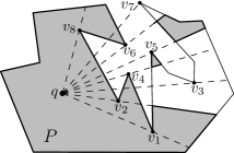
Figure 1: An example with $k=2$. The hatched regions are not $2$-visible for $q$. The vertices $v_{1},\dots,v_{8}$ are critical for $q$. More precisely, $v_{1},v_{2},v_{3},v_{6}$ are start vertices, and $v_{4},v_{5},v_{7},v_{8}$ are end vertices. $\partial P$ is partitioned into $8$ disjoint chains, e.g, the counterclockwise chain $v_{3}v_{5}$.

We fix a coordinate system with origin $q$. For $\theta\in[0,2\pi)$, we denote by $r_{\theta}$ the ray that emanates from $q$ and has CCW-angle $\theta$ with the $x$-axis. An edge of $P$ that intersects $r_{\theta}$ is called an intersecting edge of $r_{\theta}$. The edge list of $r_{\theta}$ is defined as the list of intersecting edges of $r_{\theta}$, sorted according to their intersection with $r_{\theta}$, in increasing distance from $q$. The $j^{\text{th}}$ element of this list is denoted by $e_{\theta}(j)$. We also say that $e_{\theta}(j)$ has rank $j$ in the edge list of $r_{\theta}$, or simply on $r_{\theta}$.

The angle of a vertex $v$ of $P$ refers to the angle $\theta\in[0,2\pi)$ at which $r_{\theta}$ encounters $v$. Suppose $r_{\theta}$ stabs a vertex $v$ of $P$. We call $v$ a critical vertex if its incident edges lie on the same side of $r_{\theta}$, and a non-critical vertex otherwise. We can check in constant time whether a given vertex of $P$ is critical. We use $c$ to denote the number of critical vertices in $P$. Let $v$ be a critical vertex. We call $v$ a start vertex if both incident edges lie counterclockwise of $r_{\theta}$, and an end vertex otherwise; see Figure 1. A chain is a sequence of edges of $P$ (in CW or CCW order along $\partial P$) which starts at a start vertex and ends at an end vertex and contains no other critical vertices. Note that every ray $r_{\theta}$ intersects each chain at most once. Thus, we will sometimes talk of chains that appear in the edge list of a ray $r_{\theta}$.

Suppose we continuously increase $\theta$ from $0$ to $2\pi$. The edge list of $r_{\theta}$ only changes when $r_{\theta}$ encounters a vertex $v$ of $P$. This change only involves the two edges incident to $v$. At a non-critical vertex $v$, the edge list is updated by replacing one incident edge of $v$ with the other. The other edges and their order in the edge list do not change. At a critical vertex $v$, the edge list is updated by adding or removing both incident edges of $v$, depending on whether $v$ is a start vertex or an end vertex. The other edges and their order in the edge list are not affected; see Figure 1. If $r_{\theta}$ stabs a start vertex of $P$, we define the edge list of $r_{\theta}$ to be the edge list of $r_{\theta+\varepsilon}$, for a small enough $\varepsilon>0$. If $r_{\theta}$ stabs an end vertex or a non-critical vertex of $P$, we define the edge list of $r_{\theta}$ to be the edge list of $r_{\theta-\varepsilon}$, for a small enough $\varepsilon>0$.

For any $\theta\in[0,2\pi)$, only the first $k+1$ elements in the edge list of $r_{\theta}$ are $k$-visible from $q$ in direction $\theta$. While increasing $\theta$, as long as $r_{\theta}$ does not encounter a critical vertex, the $k$-visible chains in direction $\theta$ do not change. However, if $r_{\theta}$ encounters a critical vertex $v$, then this may affect which chains are visible from $q$. This happens if at least one of the incident edges to $v$ is among the first $k+1$ elements in the edge list of $r_{\theta}$. In other words, if $v$ is $k$-visible from $q$, which means that $v$ does not lie after $e_{\theta}(k+1)$ on $r_{\theta}$. The next lemma shows that in this case a segment on $r_{\theta}$ may occur on $\partial V_{k}(P,q)$.

Lemma 2.1.

Let $\theta\in[0,2\pi)$ such that $r_{\theta}$ stabs a $k$-visible end or start vertex $v$. Then, the segment on $r_{\theta}$ between $e_{\theta}(k+2)$ and $e_{\theta}(k+3)$ is an edge of $V_{k}(P,q)$, provided that these two edges exist.

Proof.

Suppose that $v$ is a $k$-visible end vertex. As mentioned above, right after $r_{\theta}$ encounters $v$, two consecutive edges are removed from the edge list of $r_{\theta}$. Since $v$ is $k$-visible, these edges are among the first $k+2$ entries in the edge list. Thus, right after $v$, the $k$-visibility region of $q$ extends to $e_{\theta}(k+3)$ (recall that the indices refer to the situation just before $v$). Before $v$, the $k$-visibility region extends to $e_{\theta}(k+1)$. This means that the segment between $e_{\theta}(k+2)$ and $e_{\theta}(k+3)$ on $r_{\theta}$ belongs to $\partial V_{k}(P,q)$. In particular, this includes the case that $e_{\theta}(k+1)$ and $e_{\theta}(k+2)$ are incident to $v$. The situation for a $k$-visible start vertex $v$ is symmetric. Note that in this case, the indices in the edge list refer to the situation just after $v$; see Figure 2. ∎

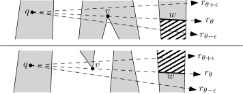
Figure 2: An example with $k=4$. The hatched regions are not 4-visible for $q$. (a) The ray $r_{\theta}$ encounters the end vertex $v$. The $4$-visibility region of $q$ right before $v$ extends to $e_{\theta}(5)$ and right after $v$ extends to $e_{\theta}(7)$. (b) The ray $r_{\theta}$ encounters the start vertex $v$. The $4$-visibility region of $q$ right before $v$ extends to $e_{\theta}(7)$ and right after $v$ extends to $e_{\theta}(5)$. The segment $w$ in both figures is the window of $r_{\theta}$.

Lemma 2.1 leads to the following definition: let $\theta\in[0,2\pi)$ such that $r_{\theta}$ stabs a $k$-visible end or start vertex $v$. The segment on $r_{\theta}$ between $e_{\theta}(k+2)$ and $e_{\theta}(k+3)$, if these edges exist, is called the window of $r_{\theta}$; see Figure 2.

Observation 2.2.

The $k$-visibility region $V_{k}(P,q)$ has $O(n)$ vertices.

Proof.

The boundary $\partial V_{k}(P,q)$ consists of subchains of $\partial P$ and of windows. Thus, a vertex of $V_{k}(P,q)$ is either a vertex of $P$ or an endpoint of a window. Since each critical vertex causes at most one window, since each window has two endpoints, and since there are at most $n$ critical vertices, the total number of vertices of $V_{k}(P,q)$ is $O(n)$. ∎

3 A Constant-Memory Algorithm

First, we assume that a constant amount of workspace is available. If the input polygon $P$ has no critical vertex, there is no window, and $V_{k}(P,q)=P$. This can be checked in $O(n)$ time by a simple scan through the input. Thus, we assume that $P$ has at least one critical vertex $v_{0}$. Again, $v_{0}$ can be found in $O(n)$ time with a single scan. We choose our coordinate system such that $q$ is the origin and such that $v_{0}$ lies on the positive $x$-axis. We number the critical vertices of $P$ as $v_{0},v_{1},\dots,v_{c-1}$ in the order that the ray $r_{\theta}$ encounters them. Let $\theta_{i}$ be the angle for $v_{i}$. We simplify our notation and write $r_{i}$ instead of $r_{\theta_{i}}$, and we let $e_{i}(j)$ denote the $j^{\text{th}}$ entry in the edge list of the ray $r_{i}$.

We start with the ray $r_{0}$, and we find the edge $e_{0}(k+1)$ in $O(kn)$ time using $O(1)$ words of workspace. For this, we perform a simple selection subroutine as follows: we scan the input $k+1$ times, and in each pass, we find the next intersecting edge of $r_{0}$ until $e_{0}(k+1)$. If $v_{0}$ is $k$-visible, i.e., if it is not after $e_{0}(k+1)$ on $r_{0}$, we report the window of $r_{0}$, as given by Lemma 2.1 (if it exists). Since the window is defined by $e_{0}(k+2)$ and $e_{0}(k+3)$, it can be found in two more scans over the input.

Next, we find $v_{1}$ by a single scan of $\partial P$. Then, we determine $e_{1}(k+1)$. This can be done in $O(n)$ time by using $e_{0}(k+1)$ as a starting point: we know that if $v_{0}$ is an end vertex, the two incident chains of $v_{0}$ disappear in the edge list of $r_{1}$. If $v_{1}$ is a start vertex, the two incident chains of $v_{1}$ appear in the edge list of $r_{1}$. All other chains are not affected, and they intersect $r_{0}$ and $r_{1}$ in the same order. Using this, we first find the edge $e^{\prime}$ that has rank $k+1$ in the edge list of the ray $r_{\theta_{0}+\varepsilon}$ just after $r_{0}$. Depending on the type and position of $v_{0}$, $e^{\prime}$ is either $e_{0}(k+1)$ or $e_{0}(k+3)$, and it can be found in $O(n)$ time. Then, by scanning $\partial P$ starting from $e^{\prime}$, we can find the edge $e^{\prime\prime}$ on the chain of $e^{\prime}$ that intersects the ray $r_{\theta_{1}-\varepsilon}$ just before $r_{1}$, again in $O(n)$ time. Depending on the type and position of $v_{1}$, the edge $e^{\prime\prime}$ is either $e_{1}(k+1)$ or $e_{1}(k+3)$. Thus, we can find $e_{1}(k+1)$ using $e^{\prime\prime}$ in $O(n)$ time; see Figure 3.

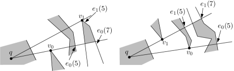
Figure 3: Two cases for going from $v_{0}$ to $v_{1}$, with $k=4$. (a) Both $v_{0}$ and $v_{1}$ are end vertices. We use $e_{0}(5)$ to find $e_{0}(7)$ and follow the chain until $e_{1}(5)$. (b) Both $v_{0}$ and $v_{1}$ are start vertices. We follow the chain of $e_{0}(5)$ until $e_{1}(7)$, and then use it to find $e_{1}(5)$. We report the window from $e_{1}(6)$ to $e_{1}(7)$.

If $v_{1}$ is $k$-visible, we report the window of $r_{1}$ in $O(n)$ time, as described above. Finally, we report the subchains of $\partial V_{k}(P,q)$ between $r_{0}$ and $r_{1}$ by scanning $\partial P$. More precisely, we walk along $\partial P$ in counterclockwise direction. Whenever we enter the counterclockwise cone between $r_{0}$ and $r_{1}$, we check whether the intersection between $\partial P$ and $r_{0}$ or $r_{1}$ occurs at or before $e_{0}(k+1)$ or $e_{1}(k+1)$, respectively. If so, we report the subchain of $\partial P$ until we leave the cone again.

We repeat this procedure until all critical vertices have been processed; see Algorithm 3.1. Here and in the following algorithms, if there are less than $k+1$ intersecting edges on $r_{i}$, we store the last intersecting edge together with its rank. We use this edge instead of $e_{i}(k+1)$, in the procedure above, to find $e_{i+1}(k+1)$ or the last intersecting edge of $r_{i+1}$ and its rank. The number of critical vertices is $c$. For each of them, we spend $O(n)$ time. Additionally, the selection subroutine for $v_{0}$ takes $O(kn)$ time. This leads to the following theorem:

input: Simple polygon $P$, point $q\in P$, $k\in\mathbb{N}$

output: The boundary of the $k$-visibility region of $q$ in $P$, $\partial V_{k}(P,q)$

1 if $P$ has no critical vertex then

2       return $\partial P$

3      

4$v_{0}\leftarrow$ a critical vertex of $P$

5 Find $e_{0}(k+1)$ using selection

6 $i\leftarrow 0$

7 repeat

8       if $v_{i}$ lies on or before $e_{i}(k+1)$ on $r_{i}$ then

9             Report the window of $r_{i}$ (if it exists)

10            

11      $v_{i+1}\leftarrow$ the next counterclockwise critical vertex after $v_{i}$

12       Find $e_{i+1}(k+1)$ using $e_{i}(k+1)$

13       Report the part of $\partial V_{k}(P,q)$ between $r_{i}$ and $r_{i+1}$

14       $i\leftarrow i+1$

15until $v_{i}=v_{0}$

Algorithm 3.1 The constant workspace algorithm for computing $V_{k}(P,q)$

Theorem 3.1.

Given a simple polygon $P$ with $n$ vertices, a point $q\in P$, and a parameter $k\in\{0,\dots,n-1\}$, we can report the $k$-visibility region of $q$ in $P$ in $O(kn+cn)$ time using $O(1)$ words of workspace, where $c$ is the number of critical vertices of $P$.

4 Time-Space Trade-Offs

In this section, we assume that we have $O(s)$ words of workspace at our disposal, and we show how to exploit this additional workspace to compute the $k$-visibility region faster. We describe two algorithms. The first algorithm is a little simpler, and it is meant to illustrate the main idea behind the trade-off. Our main contribution is in the second algorithm, which is more complicated but achieves a better running time. In the first algorithm, we process the vertices in angular order in contiguous batches of size $s$. In each iteration, we find the next batch of $s$ vertices, and using the edge list of the last processed vertex, we construct a data structure that is used to output the windows of the batch. Using the windows, we report $\partial V_{k}(P,q)$ between the first and the last ray of the batch. In the second algorithm, we improve the running time by skipping the non-critical vertices. Specifically, in each iteration, we find the next batch of $s$ adjacent critical vertices, and as before, we construct a data structure for finding the windows. We need a more involved approach in order to maintain this data structure. The next lemma shows how to obtain the contiguous batches of vertices in angular order efficiently. The procedure is taken from the work of Chan and Chen [9] (see the second paragraph in the proof of Theorem 2.1 in [9]).

Lemma 4.1.

Suppose we are given a read-only array $A$ with $n$ pairwise distinct elements from a totally ordered universe and an element $x\in A$. For any given parameter $s\in\{1,\dots,n\}$, there is an algorithm that runs in $O(n)$ time and uses $O(s)$ words of workspace and that finds the set of the first $s$ elements in $A$ that follow $x$ in the sorted order.

Proof.

Let $A_{>x}$ be the subsequence of $A$ that contains exactly the elements in $A$ that are larger than $x$. The algorithm makes a single pass over $A_{>x}$ and processes the elements in batches. In the first step, we insert the first $2s$ elements of $A_{>x}$ into our workspace (without sorting them). We select the median of these $2s$ elements using $O(s)$ time and space, and we remove the elements which are larger than the median. In the next step, we insert the next batch of $s$ elements from $A_{>x}$ into the workspace, and we again find the median of the resulting $2s$ elements and remove those elements that are larger than the median. We repeat the latter step until all the elements of $A_{>x}$ have been processed. Clearly, at the end of each step, the $s$ smallest elements of $A_{>x}$ that we have seen so far reside in memory. Since the number of steps is $O(n/s)$ and since each step needs $O(s)$ time, the running time of the algorithm is $O(n)$. By construction, it uses $O(s)$ words of workspace. ∎

Lemma 4.2.

Suppose we are given a read-only array $A$ with $n$ elements from a totally ordered universe and a number $k\in\{1,\dots,n-1\}$. For any given parameter $s\in\{1,\dots,n\}$, there is an algorithm that runs in $O\big{(}\lceil k/s\rceil n\big{)}$ time and uses $O(s)$ words of workspace and that finds the $k^{\text{th}}$ smallest element in $A$.

Proof.

We again process the elements of $A$ in batches. In the first step, we apply Lemma 4.1 to find the first batch with the $s$ smallest elements in $A$ and to put it into our workspace. This needs $O(n)$ time and $O(s)$ words of workspace. If $k\leq s$, we select the $k^{\text{th}}$ smallest element in the workspace in $O(s)$ time; otherwise, we find the largest element $x$ in the workspace, and we apply Lemma 4.1 to find the set of $s$ elements following $x$. In step $i$, we apply Lemma 4.1 to find the $i^{\text{th}}$ batch of $s$ elements in the sorted order of $A$ and to insert this set of elements into the workspace. If $k\leq i\cdot s$, we select the $(k-(i-1)s)^{\text{th}}$ smallest element in the workspace in $O(s)$ time and we output it; otherwise, we find the largest element in the workspace and we continue. The element being sought is in the $\lceil k/s\rceil^{\text{th}}$ batch. Therefore, we can find it in $O\big{(}\lceil k/s\rceil n\big{)}$ time using $O(s)$ words of workspace. ∎

In addition to the simple algorithm in Lemma 4.2, there are several other results on selection in the read-only model; see Table 1 of [10]. In particular, there is a $O(n\log{\log_{s}{n}})$ expected time randomized algorithm for selection using $O(s)$ words of workspace in the limited workspace model [8, 21]. Depending on $k$, $s$, and $n$, we will choose the latter algorithm or the algorithm that we presented in Lemma 4.2. In conclusion, the running time of selection in the limited workspace model using $O(s)$ words of workspace, denoted by $T_{\text{selection}}$, is $O(\min\{\lceil k/s\rceil n,n\log{\log_{s}{n}}\})$ expected time.

4.1 First Algorithm: Processing All the Vertices

Let $v_{0}$ be some vertex of $P$. We choose our coordinate system such that $q$ is the origin and such that $v_{0}$ lies on the positive $x$-axis. We apply Lemma 4.1 to find the batch of $s$ vertices with the smallest positive angles, and we sort them in workspace in $O(s\log s)$ time. Let $v_{1},\dots,v_{s}$ denote these vertices in sorted order. We use the selection subroutine (with $O(s)$ words of workspace) to find $e_{0}(k+1)$ on $r_{0}$, and if $v_{0}$ is a $k$-visible vertex, i.e., if it does not occur after $e_{0}(k+1)$ on $r_{0}$, we report its window (if it exists). Recall that if there are less than $k+1$ intersecting edges on $r_{0}$, we store the last intersecting edge together with its rank.

Then, we apply Lemma 4.1 four times in order to find the at most $4s+1$ intersecting edges with ranks in $\{k-2s+1,\dots,k+2s+1\}$ on $r_{0}$ (Lemma 4.1 can be applied, because we have $e_{0}(k+1)$ at hand). We insert these edges into a balanced binary search tree $T$, sorted according to their ranks on $r_{0}$. The edges in $T$ are candidates for having rank $k+1$ on the next $s$ rays $r_{1},\dots,r_{s}$. This is because, as we explained in Section 3, if $e_{i}(k+1)$ belongs to the edge list of $r_{i-1}$, there is at most one edge between $e_{i-1}(k+1)$ and $e_{i}(k+1)$ in the edge list of $r_{i-1}$. Therefore, if $e_{i}(k+1)$ appears in the edge list of $r_{0}$, there are at most $2i-1$ edges between $e_{0}(k+1)$ and $e_{i}(k+1)$ in the edge list of $r_{0}$.

Now the algorithm proceeds as follows: we go to the next vertex $v_{1}$, and we update $T$ depending on the types of $v_{0}$ and $v_{1}$: if $v_{0}$ is a non-critical vertex, we may need to exchange one incident edge of $v_{0}$ with another in $T$; if $v_{0}$ is an end vertex, we may need to remove its incident edges from $T$; and if $v_{1}$ is a start vertex, we may need to insert its incident edges into $T$. In all other case, no action is necessary. The insertion and/or deletion is performed only for the edges whose ranks are between the smallest and the largest rank in $T$ (with respect to $r_{1}$). The update of $T$ takes $O(\log s)$ time. Afterwards, we can find $e_{1}(k+1)$ and the window of $r_{1}$ (if it exists) in $O(1)$ time, using the position of $e_{0}(k+1)$ or its neighbors in $T$, as explained in Section 3. See Figure 4 for an example.

Figure 4: The first batch $v_{0},v_{1},\dots,v_{s}$ of $s$ vertices in angular order. The edge $e_{1}(3)$ is the second neighbor to the right of $e_{0}(3)$ on $r_{0}$, because $v_{0}$ is an end vertex. The edge $e_{2}(3)$ is the second neighbor to the left of $e_{1}(3)$ which is inserted in $T$ before processing $v_{2}$. The edge $e_{2}(3)$ is exchanged with $e_{3}(3)$, after processing $v_{3}$, because $v_{3}$ is a non-critical vertex.

We repeat this procedure for $v_{2},\dots,v_{s}$. We use, for $i=2,\dots,s$, the binary search tree $T$ and the previous edge $e_{i-1}(k+1)$ in order to determine the next edge $e_{i}(k+1)$ and the window of $r_{i}$. This takes $O(s\log s)$ total time. Whenever we find and report a window, we insert its endpoints into a balanced binary search tree $W$. This takes $O(\log s)$ time per window. The endpoints in $W$ are sorted according to their counterclockwise order along $\partial P$. For reporting the part of $\partial V_{k}(P,q)$ between $r_{0}$ and $r_{s}$, we use $W$ and the sequence $E=e_{0}(k+1),e_{1}(k+1),\dots,e_{s}(k+1)$ of edges of rank $k+1$.

For an edge $e$ of $P$, the $0s$-segment of $e$ is the subsegment of $e$ that lies between $r_{0}$ and $r_{s}$. If a $0s$-segment does not contain an endpoint of a window, then it is either completely $k$-visible or completely not $k$-visible. Thus, we can walk along $\partial P$ and, simultaneously, along the window endpoints in $W$. For each edge $e$ of $P$, we can check if the endpoints of the $0s$-segment of $e$ are $k$-visible or not. We can do this in $O(1)$ time using $E$. With the help of the parallel traversal of $W$, we can also check if there is a window endpoint on $e$. This takes $O(|w_{e}|)$ time, where $|w_{e}|$ is the number of window endpoints on $e$. With this information, we can report the $k$-visible subsegments of the $0s$-segment of $e$. Since there are $O(n)$ window endpoints by Observation 2.2, and since we check each window endpoint once, it follows that we need $O(n)$ time to report the $k$-visible part of $\partial P$ between $r_{0}$ and $r_{s}$.

After processing $v_{0},\dots,v_{s}$, we apply Lemma 4.1 to find the next batch of $s$ vertices following $v_{s}$ in angular order. We sort them in $O(s\log s)$ time, using $O(s)$ words of workspace. The search tree $T$ for the previous batch is not useful anymore, because it does not necessarily contain any right or left neighbor of $e_{s}(k+1)$ on $r_{s}$. Applying Lemma 4.1 four times as before, we find the at most $4s+1$ intersecting edges with ranks in $\{k-2s+1,\dots,k+2s+1\}$ on $r_{s}$, and we insert them into $T$. Then, as before, for each $s<i\leq 2s$, we find $e_{i}(k+1)$ and its corresponding window while maintaining $T$, $W$, and $E$. After that, we report the $k$-visible part of $\partial P$ between $r_{s}$ and $r_{2s}$, where $r_{2s}$ is the ray for the last vertex in the batch, in sorted order. If $n$ is not divisible by $s$, the last batch wraps around, taking the indices modulo $n$, but we report only the part of $\partial V_{k}(P,q)$ before $r_{n}=r_{0}$; see Algorithm 4.1.

input: Simple polygon $P$, point $q\in P$, $k\in\mathbb{N}$, $1\leq s\leq n$

output: The boundary of $k$-visibility region of $q$ in $P$, $\partial V_{k}(P,q)$

1 $v_{0}\leftarrow$ a vertex of $P$

2 $E\leftarrow\langle e_{0}(k+1)\rangle$ (using the selection subroutine with $O(s)$ workspace)

3 $T$, $W\leftarrow$ an empty balanced binary search tree

4 $i\leftarrow 0$

5 repeat

6       $v_{i+1},\dots,v_{i+s}\leftarrow$ sorted list of $s$ vertices following $v_{i}$ in angular order

7       $T\leftarrow\text{at most }4s+1\text{ edges with rank in }\{k-2s+1,\dots,k+2s+1\}\text{ on }r_{i}$

8       for $j=i$ to $i+s-1$ do

9             if $v_{j}$ lies on or before $e_{j}(k+1)$ on $r_{j}$ then

10                   Report the window of $r_{j}$ (if it exists)

11                   Insert the endpoints of the window into $W$ (according to their position on $\partial P$)

12                  

13            Update $T$ according to the types of $v_{j}$ and $v_{j+1}$

14             $E.\text{append}(e_{j+1}(k+1))$ (find it using $e_{j}(k+1)$ and $T$)

15            

16      Report the part of $\partial V_{k}(P,q)$ between $r_{i}$ and $r_{\min\{i+s,n\}}$ (using $W$ and $E$)

17       $i\leftarrow i+s$

18      

19until $i\geq n$

Algorithm 4.1 Computing $\partial V_{k}(P,q)$ using $O(s)$ words of workspace

Overall, we need $O(n+s\log s)$ time for a batch. We repeat this procedure for $O(n/s)$ iterations, until all vertices are processed. Moreover, we run the selection subroutine in the first batch. Thus, the running time of the algorithm is $O(n/s(n+s\log{s}))+T_{\text{selection}}$. Since $T_{\text{selection}}$ is dominated by the other terms, we obtain the following theorem.

Theorem 4.3.

Let $s\in\{1,\dots,n\}$. Given a simple polygon $P$ with $n$ vertices in a read-only array, a point $q\in P$ and a parameter $k\in\{0,\dots,n-1\}$, we can report the $k$-visibility region of $q$ in $P$ in $O(n^{2}/s+n\log{s})$ time using $O(s)$ words of workspace.

4.2 Second Algorithm: Processing only the Critical Vertices

As in Section 4.1, we process the vertices in batches, but now we focus only on the critical vertices. The new algorithm is similar to the algorithm in Section 4.1, but it handles the data structure for the intersecting edges differently. In each iteration, we find the next batch of $s$ critical vertices, and we sort them in $O(s\log s)$ time using $O(s)$ words of workspace. As in the previous algorithm, we construct a data structure $T$ that contains the possible candidates for the edges of rank $k+1$ on the rays for the $s$ critical vertices of the batch. In each step, we process the next critical vertex. We use $T$ to find the corresponding window, and we update $T$. For updating $T$, we consider only the changes in the edge list that are caused by the critical vertices. This is because the non-critical vertices do not change the chains that appear in the edge list of the ray; they only affect the actual edge that intersects it.

More precisely, we use a lazy strategy for updating $T$: instead of always maintaining the edges that intersect the current ray, we only store some edge on their corresponding chains, and we determine the precise intersecting edges only when the need arises; see below, and Figure 5 for an illustration. After finding all the windows of the batch, we report the $k$-visible part of $\partial P$ between the first and the last ray of the batch.

As in Section 3, if $P$ has no critical vertex, then $V_{k}(P,q)=P$. This can be checked in $O(n)$ time by a simple scan through the input. Thus, we let $v_{0}$ be some critical vertex, and we choose our coordinate system such that $q$ is the origin and such that $v_{0}$ lies on the positive $x$-axis. In the first iteration, we compute $v_{1},\dots,v_{s}$, the list of $s$ critical vertices after $v_{0}$, sorted in angular order. Using Lemma 4.1 and a traditional sorting algorithm, this takes $O(n+s\log s)$ time and $O(s)$ words of workspace.

Then, we process one critical vertex in each step. In step $0$, we find $e_{0}(k+1)$ using our selection subroutine, and the at most $4s+1$ intersecting edges with rank in $\{k-2s+1,\dots,k+2s+1\}$ on $r_{0}$. We insert them into a balanced binary search tree $T$, ordered according to their rank on $r_{0}$. This takes $T_{\text{selection}}+O(n+s\log s)$ time. We use $e_{0}(k+1)$ and $T$ to find and report the window of $r_{0}$ (if it exists).

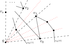
Figure 5: The first batch $v_{0},v_{1},\dots,v_{s}$ of $s$ critical vertices in angular order. The edge $e_{0}(1)$ intersects only $r_{0}$ and $r_{1}$. However, it is in the edge list of $r_{2}$ as a representative for $e_{2}(1)$. Similarly, $e_{0}(4)$ is a representative for $e_{1}(2)$ in the edge list of $r_{1}$.

In step $1$, we update $T$ according to the types of $v_{0}$ and $v_{1}$, so that $T$ contains representatives for the chains that intersect $r_{1}$: if $v_{0}$ is an end vertex, and if its incident edges are in $T$, we remove those edges from $T$; if $v_{1}$ is a start vertex, we insert the two incident edges of $v_{1}$ (as representatives of the corresponding chains) into $T$, provided that their ranks on $r_{1}$ are in the correct rank interval for the edges in $T$. For finding the rank of the incident edges of $v_{1}$ on $r_{1}$, we perform a search in $T$ to compare the positions of these edges and the elements of $T$ on $r_{1}$. Whenever a comparison needs to be done with an edge $e$ stored in $T$, we check whether $e$ intersects $r_{1}$. If not, we follow the corresponding chain of $e$ until we find such an edge. Thus, it takes $O(\log s+n_{1}^{\prime})$ time to update $T$, where $n_{1}^{\prime}$ denotes the number of non-critical vertices that are traversed to find the correct edges for comparisons during the update operations.

Now, $T$ contains at most $4s+1$ intersecting chains of $r_{1}$. To determine $e_{1}(k+1)$, we walk along the chain of either $e_{0}(k+1)$ or its neighbors in $T$, until we meet the edge that intersects $r_{1}$. Having $e_{1}(k+1)$ and $T$, we find and report the window of $r_{1}$ (if it exists), again using our lazy strategy. Finding $e_{1}(k+1)$ and the window of $r_{1}$ takes $O(n_{1}^{\prime\prime})$ time, where $n_{1}^{\prime\prime}$ is the number of non-critical vertices that are traversed during the search.

In step $i=\{2,\dots,c-1\}$, we repeat the same procedure as in step $1$. We update $T$ for the edges that are incident to the critical vertices $v_{i-1}$ and $v_{i}$. The only difference is that, if $v_{i-1}$ is an end vertex, checking whether its chains are in $T$, and identifying their representative edge in $T$, are not as straightforward as in step $1$. The problem is that we do not know which edge of each chain has been stored in $T$ as its representative. To resolve this problem, for any chain $C$ in $T$, we additionally store another edge of $C$ that is called the guide edge and that is defined as follows: if $C$ intersects $r_{0}$, the edge on $C$ that intersects $r_{0}$ is a type $1$ guide edge; and if $C$ has been inserted into $T$ in one of the steps $2,\dots,i-1$, the first edge of $C$ is a type $2$ guide edge.

We store the type $1$ guide edges in an array $G_{1}$, sorted according to their rank on $r_{0}$, i.e., we copy the sorted elements of $T$ in step $0$ into $G_{1}$. The type $2$ guide edges are stored in another array $G_{2}$, sorted according to the step in which they have been inserted into $T$, i.e., the angle of the start vertex of the chain. Therefore, in each step that new edges are inserted into $T$, those edges will also be added to $G_{2}$ in $O(1)$ time. The keys for the elements in $G_{2}$ will be the corresponding rays $r_{i}$. (since both arrays have length $O(s)$, we can reserve memory for them in advance. The elements in $G_{1}$ and $G_{2}$ have cross-pointers to their corresponding entries in $T$.

To find the corresponding elements of the chains of an end vertex $v_{i-1}$ in $T$, we walk backward on each chain, until we either encounter an edge that intersects $r_{0}$ (a type 1 guide edge), or the first edge of that chain (a type 2 guide edge). Then, by a binary search in $G_{1}$ or $G_{2}$ in $O(\log s)$ time, and using the cross-pointer to the elements in $T$, we identify the corresponding entries in $T$. Therefore, we can remove them from $T$ in $O(\log s)$ time. Now, $T$ contains the chain list of $v_{i}$ and can be used to find $e_{i}(k+1)$ with the help of $e_{i-1}(k+1)$. Finally, we report the window of $r_{i}$ (if it exists), as in step $1$. In total, processing the changes in $T$ for a batch takes $O(s\log s+n^{\prime})$ time, where $n^{\prime}$ is the number of non-critical vertices that lie between $r_{0}$ and $r_{s}$.

While processing the batch, we insert all $e_{i}(k+1)$, $0\leq i\leq s$, into $E$. Also, whenever we find and report a window, we insert its endpoints, sorted according to their counterclockwise order along $\partial P$, into a balanced binary search tree $W$, in $O(\log s)$ time. After processing all the vertices of the batch, we use $W$ and $E$ to report the part of $\partial V_{k}(P,q)$ between $r_{0}$ and $r_{s}$, as in Section 4.1. The only difference is that now we keep track of the visibility of the whole chains between $r_{0}$ and $r_{s}$ instead of individual edges. As before, this takes $O(n)$ time.

In the subsequent iteration, we repeat the same procedure for the next batch of $s$ critical vertices. We repeat until all critical vertices are processed; see Algorithm 4.2. By construction, each non-critical vertex is handled in exactly one iteration. Since there are $O(c/s)$ iterations, updating $T$ takes $O(c\log s+n)$ time in total. All together, we get a total running time of $O(cn/s+c\log s)$, in addition to $T_{\text{selection}}$ in the first batch. This leads to the following theorem:

Theorem 4.4.

Let $s\in\{1,\dots,n\}$. Given a simple polygon $P$ with $n$ vertices in a read-only array, a point $q\in P$ and a parameter $k\in\{0,\dots,n-1\}$, we can report the $k$-visibility region of $q$ in $P$ in $O(cn/s+c\log{s}+\min\{\lceil k/s\rceil n,n\log{\log_{s}{n}}\})$ expected time using $O(s)$ words of workspace, where $c$ is the number of critical vertices of $P$ for $q$.

input: Simple polygon $P$, point $q\in P$, $k\in\mathbb{N}$, $1\leq s\leq n$

output: The boundary of $k$-visibility region of $q$ in $P$, $\partial V_{k}(P,q)$

1 $v_{0}\leftarrow$ a critical vertex of $P$

2 $E\leftarrow\langle e_{0}(k+1)\rangle$ (using the selection subroutine with $O(s)$ workspace)

3 $T$, $W\leftarrow$ an empty balanced binary search tree

4 $G_{1},G_{2}\leftarrow\langle\rangle$

5 $i\leftarrow 0$

6 repeat

7       $v_{i+1},\dots,v_{i+s}\leftarrow$ sorted list of $s$ critical vertices following $v_{i}$ in angular order

8       $T\leftarrow\text{at most }4s+1\text{ edges with rank in }\{k-2s+1,\dots,k+2s+1\}\text{ on }r_{i}$

9       $G_{1}\leftarrow$ the sorted elements of $T$

10       for $j=i$ to $i+s-1$ do

11             if $v_{j}$ lies on or before $e_{j}(k+1)$ on $r_{j}$ then

12                   Report the window of $r_{j}$ (if it exists)

13                   Insert the endpoints of the window into $W$ (sorted by position on $\partial P$)

14                  

15            if $v_{j}$ is an end vertex then

16                   Find the guide edges of chains of $v_{j}$ (by walking along the chains)

17                   if the guide edges exist in $G_{1}$ or $G_{2}$ then

18                         Use their cross-pointers to find the corresponding elements in $T$

19                         Remove those corresponding elements from $T$

20            if $v_{j+1}$ is a start vertex then

21                   repeat

22                         Take the next edge $e$ along the search path in $T$

23                         if $e$ does not intersect $r_{j+1}$ then

24                               Walk along the chain of $e$ until the edge $e^{\prime}$ that intersects $r_{j+1}$

25                               Exchange $e$ with $e^{\prime}$ in $T$

26                              

27                        Compare the position of $e$ with $v_{j+1}$ on $r_{j+1}$

28                        

29                  until rank of the chains of $v_{j+1}$ on $r_{j+1}$ are determined

30                  if the rank of the chains of $v_{j+1}$ are valid for $T$ then

31                         Insert the chains of $v_{j+1}$ into $T$ according to their rank on $r_{j+1}$

32                         Append the chains of $v_{j+1}$ to $G_{2}$

33                        

34            Find $e_{j+1}(k+1)$ by walking along $e_{j}(k+1)$ or its neighbors in $T$

35             Append $e_{j+1}(k+1)$ to $E$

36            

37      Report subchains of $\partial V_{k}(P,q)$ between $r_{i}$ and $r_{\min\{i+s,n\}}$ (using $W$ and $E$)

38       $i\leftarrow i+s$

39      

40until $i\geq n$

Algorithm 4.2 Computing $\partial V_{k}(P,q)$ using $O(s)$ words of workspace

5 Variants and Extensions

Our results can be extended in several ways; for example, computing the $k$-visibility region of a point $q$ inside a polygon $P$, where $P$ may have holes, or computing the $k$-visibility region of a point $q$ in a planar arrangement of $n$ non-crossing segments inside a bounding box (the bounding box is only for bounding the $k$-visibility region). Concerning the first extension, all the properties we showed to hold for the algorithms for simple polygons also hold for the case with holes. The only noteworthy issue is the use of $\partial P$ to report the $k$-visible segments of $\partial P$. In the case of polygons with holes, after walking on the outer part of $\partial P$, we walk on the boundaries of the holes one by one and we apply the same procedures for them. If there is no window on the boundary of a hole, then it is either completely $k$-visible or completely non-$k$-visible. For such a hole, we check if it is $k$-visible and, if so, we report it completely. This leads to the following corollary:

Corollary 5.1.

Let $s\in\{1,\dots,n\}$. Given a polygon $P$ with $h\geq 0$ holes and $n$ vertices in a read-only array, a point $q\in P$ and a parameter $k\in\{0,\dots,n-1\}$, we can report the $k$-visibility region of $q$ in $P$ in $O(cn/s+c\log{s}+\min\{\lceil k/s\rceil n,n\log{\log_{s}{n}}\})$ expected time using $O(s)$ words of workspace. Here, $c$ is the number of critical vertices of $P$ for the point $q$.

Concerning the second problem, for a planar arrangement of $n$ non-crossing segments inside a bounding box, the output consists of the $k$-visible parts of the segments. All the segments endpoints are critical vertices and should be processed. In the parts of the algorithm where a walk on the boundary is needed, a sequential scan of the input leads to similar results. Similarly, there may be some segments with no window endpoints. For these, we only need to check visibility of an endpoint to decide whether they are completely $k$-visible or completely non-$k$-visible. This leads to the following corollary:

Corollary 5.2.

Let $s\in\{1,\dots,n\}$. Given a set $S$ of $n$ non-crossing planar segments in a read-only array that lie in a bounding box $B$, a point $q\in B$ and a parameter $k\in\{0,\dots,n-1\}$, there is an algorithm that reports the $k$-visible subsets of segments in $S$ from $q$ in $O(n^{2}/s+n\log{s})$ time using $O(s)$ words of workspace.

6 Conclusion

We have proposed algorithms for a class of $k$-visibility problems in the limited workspace model, and we have provided time-space trade-offs for these problems. We leave it as an open question whether the presented algorithms are optimal. Also, it would be interesting to see whether there exists an output sensitive algorithm whose running time depends on the number of windows in the $k$-visibility region, instead of the critical vertices in the input polygon.

Finally, our ideas are also applicable to the slightly different definition of $k$-visibility used by Bajuelos et al. [4]. Thus, our techniques can be used to improve their result, achieving $O(n\log n)$ running time if $O(n)$ words of workspace are available.

References

- [1] M. Abrahamsen. An optimal algorithm computing edge-to-edge visibility in a simple polygon. In Proc. 25th Canad. Conf. Comput. Geom. (CCCG), 2013.
- [2] O. Aichholzer, R. Fabila Monroy, D. Flores Peñaloza, T. Hackl, C. Huemer, J. Urrutia Galicia, and B. Vogtenhuber. Modem illumination of monotone polygons. In Proc. 25th European Workshop Comput. Geom. (EWCG), pages 167–170, 2009.
- [3] T. Asano, K. Buchin, M. Buchin, M. Korman, W. Mulzer, G. Rote, and A. Schulz. Memory-constrained algorithms for simple polygons. Comput. Geom. Theory Appl., 46(8):959–969, 2013.
- [4] A. L. Bajuelos, S. Canales, G. Hernández-Peñalver, and A. M. Martins. A hybrid metaheuristic strategy for covering with wireless devices. Journal of Universal Computer Science, 18(14):1906–1932, 2012.
- [5] B. Ballinger, N. Benbernou, P. Bose, M. Damian, E. D. Demaine, V. Dujmovic, R. Y. Flatland, F. Hurtado, J. Iacono, A. Lubiw, P. Morin, V. Sacristán Adinolfi, D. L. Souvaine, and R. Uehara. Coverage with -transmitters in the presence of obstacles. Journal of Combinatorial Optimization, 25(2):208–233, 2013.
- [6] L. Barba, M. Korman, S. Langerman, K. Sadakane, and R. I. Silveira. Space-time trade-offs for stack-based algorithms. Algorithmica, 72(4):1097–1129, 2015.
- [7] L. Barba, M. Korman, S. Langerman, and R. I. Silveira. Computing a visibility polygon using few variables. Comput. Geom. Theory Appl., 47(9):918–926, 2014.
- [8] T. M. Chan. Comparison-based time-space lower bounds for selection. ACM Transactions on Algorithms, 6(2):26, 2010.
- [9] T. M. Chan and E. Y. Chen. Multi-pass geometric algorithms. Discrete Comput. Geom., 37(1):79–102, 2007.
- [10] T. M. Chan, J. I. Munro, and V. Raman. Selection and sorting in the restore model. In Proc. 25th Annu. ACM-SIAM Sympos. Discrete Algorithms (SODA), pages 995–1004, 2014.
- [11] A. M. Dean, W. Evans, E. Gethner, J. D. Laison, M. A. Safari, and W. T. Trotter. Bar -visibility graphs: Bounds on the number of edges, chromatic number, and thickness. In Proc. 13th Int. Symp. Graph Drawing (GD), pages 73–82, 2005.
- [12] J. A. Dean, A. Lingas, and J.-R. Sack. Recognizing polygons, or how to spy. The Visual Computer, 3(6):344–355, 1988.
- [13] D. Eppstein, M. T. Goodrich, and N. Sitchinava. Guard placement for efficient point-in-polygon proofs. In Proc. 23rd Annu. Sympos. Comput. Geom. (SoCG), pages 27–36, 2007.
- [14] R. Fabila-Monroy, A. R. Vargas, and J. Urrutia. On modem illumination problems. In Proc. 13th Encuentros de Geometría Computacional (EGC), 2009.
- [15] S. Felsner and M. Massow. Parameters of bar -visibility graphs. J. Graph. Alg. Appl., 12(1):5–27, 2008.
- [16] R. Fulek, A. F. Holmsen, and J. Pach. Intersecting convex sets by rays. Discrete Comput. Geom., 42(3):343–358, 2009.
- [17] S. K. Ghosh. Visibility algorithms in the plane. Cambridge University Press, 2007.
- [18] S. G. Hartke, J. Vandenbussche, and P. Wenger. Further results on bar -visibility graphs. SIAM J. on Discrete Mathematics, 21(2):523–531, 2007.
- [19] B. Joe and R. B. Simpson. Corrections to Lee’s visibility polygon algorithm. BIT Numerical Mathematics, 27(4):458–473, 1987.
- [20] N. Mouawad and T. C. Shermer. The superman problem. The Visual Computer, 10(8):459–473, 1994.
- [21] J. I. Munro and V. Raman. Selection from read-only memory and sorting with minimum data movement. Theoret. Comput. Sci., 165(2):311–323, 1996.
- [22] J. O’Rourke. Computational geometry column 52. ACM SIGACT News, 43(1):82–85, 2012.