Eigenstate Thermalization Hypothesis and Quantum Jarzynski Relation for Pure Initial States

Abstract

Since the first suggestion of the Jarzynski equality many derivations of this equality have been presented in both, the classical and the quantum context. While the approaches and settings greatly differ from one to another, they all appear to rely on the initial state being a thermal Gibbs state. Here, we present an investigation of work distributions in driven isolated quantum systems, starting off from pure states that are close to energy eigenstates of the initial Hamiltonian. We find that, for the nonintegrable system in quest, the Jarzynski equality is fulfilled to good accuracy.

Introduction. The last decades have witnessed a renewed interest in the old question if and how closed finite quantum systems approach thermal equilibrium. Equilibration and thermalization have been theoretically discussed for both, fairly abstract Popescu et al. (2006); Goldstein et al. (2006); Reimann (2008, 2015); Eisert et al. (2015); Gogolin and Eisert (2015) and more specific systems of condensed-matter type Rigol et al. (2008); Steinigeweg et al. (2013); Beugeling et al. (2014); Steinigeweg et al. (2014a). Key concepts in this discussion are typicality (or concentration of measure) and the eigenstate thermalization hypothesis (ETH). With the advent of experiments on ultracold atoms, some of the theoretical results have even become testable. As of today, the mere existence of some sort of equilibrium in closed quantum system has been the most widely addressed question. However, lately the dynamical approach to equilibrium has been intensely investigated Malabarba et al. (2014); Reimann (2016). Here, crucial questions are relaxation times but also the degree of agreement of quantum dynamics with standard statistical relaxation concepts like master or Fokker-Planck equations, stochastic processes, etc. Niemeyer et al. (2014); Gemmer and Steinigeweg (2014); Schmidtke and Gemmer (2016) The crucial feature that discriminates these types of analysis from standard open-systems concepts, like quantum master equations, is the fact that the statistical dynamics emerge from the systems themselves, i.e., are not induced by any bath.

Also fluctuation theorems have been and continue to be a central topic in the field of statistical mechanics Seifert (2008). The Jarzynski relation (JR), making general statements on work that has to be invested to drive processes also and especially far from equilibrium, is a prime example of such a fluctuation theorem. Many derivations of the JR from various starting grounds have been presented. These include classical Hamiltonian dynamics, stochastic dynamics such as Langevin or master equations, as well as quantum mechanical starting points Seifert (2008); Esposito et al. (2009); Jarzynski (2011); Roncaglia et al. (2014); Hänggi and Talkner (2015). However, all these derivations assume that the system that is acted on with some kind of “force” is strictly in a Gibbsian equilibrium state before the process starts. This starting point differs from the progresses in the field of thermalization: There, the general features of thermodynamical relaxation are found to emerge entirely from the system itself without the necessity of evoking external baths or specifying initial states in detail. Clearly, the preparation of a strictly Gibbsian initial state requires the coupling to a bath prior to starting the process.

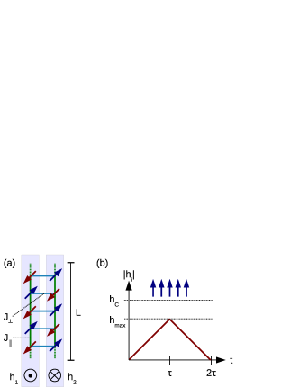
Figure 1: Sketch of the (a) Heisenberg $S=1/2$ ladder studied and (b) the time-dependent magnetic field applied.

In this Letter, we study the question whether or not the JR is valid with a system starting in a state other than a Gibbs state. Since counterexamples can be constructed, any affirmative answer cannot hold for any quantum system and for any process protocol. In fact, previous works Talkner et al. (2008); Campisi (2008); Talkner et al. (2013); Campisi et al. (2011) have shown that, when the initial state is microcanonical, the JR does not follow, but a related entropy-from-work relation emerges instead. The question remains, however, if and under what conditions the JR holds approximately for non-canonical initial states. Thus, the emphasis in the search for the origins of the JR’s validity is shifted from specifying the initial state to specifying the nature of the system.

JR and ETH. To further clarify this, consider the standard setup of the quantum JR for closed systems. It is based on a two-measurement scheme: If the system is at energy $E_{\text{ini}}$ before the process, then there is a conditional probability $T=T(E_{\text{fin}}|E_{\text{ini}},\lambda(t))$ (with $\lambda(t)$ being the protocol) to find the system at $E_{\text{fin}}$ after the process not . Let $W=E_{\text{fin}}-E_{\text{ini}}$ be the work associated with this transition. The average of the exponentiated work $\langle e^{-\beta W}\rangle$ can now be written as

$$\langle e^{-\beta W}\rangle=\!\sum_{E_{\text{fin}},E_{\text{ini}}}\!T\,e^{-\beta(E_{\text{fin}}-E_{\text{ini}})}P_{\text{ini}}(E_{\text{ini}})\,.$$ (1)

Obviously, $\langle e^{-\beta W}\rangle$ depends on $P_{\text{ini}}(E_{\text{ini}})$. It is well-known that the JR $\langle e^{-\beta W}\rangle=e^{-\beta\Delta F}$ always holds for initial Gibbs states $P_{\text{ini}}(E_{\text{ini}})\propto e^{-\beta E_{\text{ini}}}$, regardless of the system and the protocol. Much less is known on other initial states, e.g., initial energy eigenstates $P_{\text{ini}}(E_{\text{ini}})\approx\delta_{E_{\text{ini}},E_{n}}$ with $E_{n}$ being the energy of an eigenstate. These states are in center of our Letter.

It is very important to note that this question can be recast as a question on the validity of the ETH in a specific sense: As shown in Talkner et al. (2008), the average exponentiated work can be written as the expectation value

$$\langle e^{-\beta W}\rangle=\langle e^{-\beta H^{H}_{\text{fin}}}e^{\beta H_{\text{ini}}}\rangle_{\text{diag}}\,,$$ (2)

where $H_{\text{fin/ini}}$ are the final/initial Hamiltonian (with the index $H$ indicating the Heisenberg picture) and $\langle\cdots\rangle_{\text{diag}}$ denotes the average over the diagonal part of the initial density matrix w.r.t. the eigenbasis of $H_{\text{ini}}$ Talkner et al. (2008). Let $\langle\cdots\rangle_{\text{can}/\text{mic}}$ denote averages over canonical/microcanonical states, which are both diagonal in the above sense. While the standard JR $\langle e^{-\beta W}\rangle=\langle e^{-\beta H^{H}_{\text{fin}}}e^{-\beta H_{\text{ini}}}\rangle_{\text{can}}=e^{-\beta\Delta F}$ always holds, our questions can be reformulated as

$$\langle e^{-\beta H^{H}_{\text{fin}}}e^{\beta H_{\text{ini}}}\rangle_{\text{mic}}\stackrel{{\scriptstyle?}}{{=}}\langle e^{-\beta H^{H}_{\text{fin}}}e^{\beta H_{\text{ini}}}\rangle_{\text{can}}\,.$$ (3)

The validity of this equation is claimed by the ETH (even though the operator in the average is non-Hermitian). Since each protocol yields a different $H^{H}_{\text{fin}}$, the JR’s validity for microcanonical states is equivalent to the ETH’s validity for a set of different operators. So far, however, no general principle guarantees the applicability of the ETH, except for large quantum systems with a direct classical counterpart Srednicki (1994) or systems involving random matrices Deutsch (1991). While the ETH is expected to hold for non-integrable systems and few-body observables, $e^{-\beta H^{H}_{\text{fin}}}e^{\beta H_{\text{ini}}}$ is not such an operator. Thus, investigating the JR’s validity for microcanonical states is an highly non-trivial endeavor.

In this Letter, we use numerical methods to prepare an energetically firmly concentrated initial state and to propagate it according to the Schrödinger equation for a complex spin system with a strongly time-dependent Hamiltonian. Due to the initial state being sharp in energy, the eventual energy-probability distribution is interpreted as a work-probability distribution and thus checked for agreement with the JR, including a careful finite-size scaling. As there is no thermal initial state, we use for the inverse temperature $\beta$ in the JR the standard definition $\text{d}S/\text{d}E=\beta$ and resort to the microcanonical entropy $S=\ln n(E)$, where $n(E)$ is the density of energy eigenstates (DOS). Thus, $\beta$ depends on the spectrum. Since $\beta$ also depends on $E$, we evaluate $\beta$ at the initial energy $E_{\text{ini}}$.

Spin model and time-dependent magnetic field. The choice of our specific spin model including all its parameters roots in its being a prime example for the emergence of thermodynamical behavior in closed, small quantum systems. The quantum dynamics of certain observables have been found to be in remarkable accord with an irreversible Fokker-Plank equation for the undriven system and with a Markovian stochastic process in a more detailed sense Niemeyer et al. (2014).

As shown in Fig. 1, we study an anisotropic spin-$1/2$ Heisenberg ladder with the rung coupling being significantly weaker than the leg coupling. Specifically, the Hamiltonian $H=J_{\parallel}H_{\parallel}+J_{\perp}H_{\perp}$ consists of a leg part $H_{\parallel}$ and a rung part $H_{\perp}$,

$$H_{\parallel}\!\! = \!\!\sum_{i=1}^{L-1}\sum_{k=1}^{2}S_{i,k}^{x}S_{i+1,k}^{x}+S_{i,k}^{y}S_{i+1,k}^{y}+\Delta S_{i,k}^{z}S_{i+1,k}^{z}\,,$$

$$H_{\perp}\!\! = \!\!\sum_{i=1}^{L}S_{i,1}^{x}S_{i+1,2}^{x}+S_{i,1}^{y}S_{i+1,2}^{y}+\Delta S_{i,1}^{z}S_{i+1,2}^{z}\,,$$ (4)

where $S_{i,k}^{x,y,z}$ are spin-$1/2$ operators at site $(i,k)$. $J_{\parallel,\perp}>0$ are antiferromagnetic exchange coupling constants with $J_{\perp}=0.2\,J_{\parallel}$, $\Delta=0.6$ is the exchange anisotropy in the $z$ direction, and $L$ is the number of sites in each leg. We set $J_{\parallel}=1$ throughout this work.

A magnetic field ($h$) is turned on once the time evolution starts. The field is uniform along each individual leg, pointing in the positive $z$ direction on one leg and in the negative $z$ direction on the other. This field is linearly ramped up in time from zero to $h_{max}$ for a certain time $\tau$, and then linearly ramped down for the same time with the same slope. Thus, the field starts of at zero and ends at zero, i.e., initial and final Hamiltonian are identical. More precisely, we model the field by

$$h(t)=-h\,f(t)\,(S^{z}_{1}-S^{z}_{2})\,,$$ (5)

where $S^{z}_{k}=\sum_{i=1}^{L}S^{z}_{i,k}$, $f(t)=t/\tau$ for $0<t\leq\tau$, and $f(t)=2-t/\tau$ for $\tau<t\leq 2\tau$. The full Hamiltonian is $H_{\text{tot}}(t)=H+h(t)$. We choose the field strength $h=0.5$ for all simulations and vary the sweep time $\tau$.

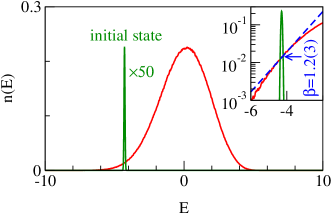
Figure 2: DOS $n(E)$ for the Heisenberg $S=1/2$ ladder in Eq. (Eigenstate Thermalization Hypothesis and Quantum Jarzynski Relation for Pure Initial States) with $J_{\perp}=0.2\,J_{\parallel}$, $\Delta=0.6$, and $L=11$. Due to the method used to obtain the numerical data, the energy resolution $0.007(6)$ is high but finite SM . The initial state prepared is also indicated. Inset: The same as the main panel but in a semi-log plot and with the inverse temperature $\beta=1.2(3)$ indicated.

To specify a quantity that plays the role of temperature, we must have information on the DOS of $H$. Since the numerical diagonalization of $H$ is unfeasible for the system sizes we are interested in, we resort to the numerical method described in Hams and De Raedt (2000a). This method is incapable of resolving individual energy eigenvalues but captures rather accurately the coarser features of the DOS SM . The result for our Hamiltonian is displayed in Fig. 2.

We choose the initial energy $E_{\text{ini}}$ to locate the process at a non-peculiar temperature regime, i.e., neither extremely high nor very low (nor negative) temperatures but an intermediate regime on the natural scale of the model: $\beta\sim 1/J_{\parallel}$. To this end, we prepare an initial state that is energetically firmly concentrated at $E_{\text{ini}}=-4.2(8)$ for $L=11$. Using the definition $\beta=\text{d}/\text{d}E\ln n(E)$ yields $\beta=1.2(3)$. It is worth pointing out that, in this energy regime, $\beta$ does not vary much on an interval of ca. $2J_{\parallel}$, which is about the overall scale of the work required for our process.

Preparation and characterization of the initial state. We prepare a state of the form

$$\left|\Psi(a,E_{\text{ini}})\right>=\frac{e^{-a(H-E_{\text{ini}})^{2}/4}\left|\Phi\right>}{\left<\Phi\right|e^{-a(H-E_{\text{ini}})^{2}/2}\left|\Phi\right>}\,,$$ (6)

where $|\Phi\rangle$ is a random state drawn according to the Haar measure on the total Hilbert space. Obviously, $\left|\Psi(a,E_{\text{ini}})\right>$ is always centered at the energy $E_{\text{ini}}$ with a variance $\propto 1/a$. Clearly, since $|\Phi\rangle$ is random, any quantity calculated from $\left|\Psi(a,E_{\text{ini}})\right>$ is random. However, as shown (and applied Steinigeweg et al. (2014a, b, 2016)) in the context of typicality, the average $\bar{Q}$ of any quantity $Q$ calculated from $\left|\Psi(a,E_{\text{ini}})\right>$ equals the $Q$ calculated from the mixed state $\rho\propto e^{-a(H-E_{\text{ini}})^{2}/2}$. Moreover, the “error” $\epsilon^{2}=\bar{Q^{2}}-\bar{Q}^{2}$ scales as $\epsilon\propto\text{Tr}\{e^{-a(H-E_{\text{ini}})^{2}/2})\}^{-1/2}$ and is very small if the Hilbert space is large (but $a$ is not too large). Investing with reasonable computational effort, we are able to reach $a=1000$. In this regime, $\epsilon$ is negligibly small SM .

Using the same method as for calculating the DOS, we visualize the probability distribution of a state $\left|\Psi(a,E_{\text{ini}})\right>$ in Fig. 2. Clearly, this distribution is firmly concentrated at $E_{\text{ini}}=-4.2(8)$.

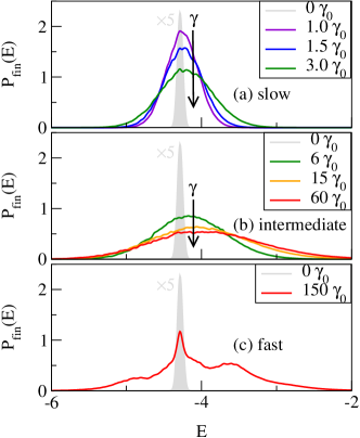
Figure 3: Probability distribution $P_{\text{fin}}(E)$ of the final state for (a) weak, (b) intermediate, and (c) fast driving. (Remaining parameters are identical to Fig. 2.) Due to the initial state being almost an energy eigenstate, this distribution almost coincides with the probability distribution of work.

Process, final energy distribution, and JR. Now, we perform the simulation of the actual process. To this end, we propagate $\left|{\Psi(a,E_{\text{ini}})}\right>$ in time according to the Schrödinger equation using the time-dependent Hamiltonian $H_{\text{tot}}(t)=H+h(t)$ SM . We do so for different sweep rates $\gamma=1/(2\tau)$, ranging from slow driving $\gamma_{0}=2.6\cdot 10^{-4}$ to fast driving at $\gamma=150\gamma_{0}$. This yields a set of final energy-probability distributions $P_{\text{fin}}(E,\gamma)$, see Fig. 3. Clearly, these distributions shift towards higher energies and broaden with increasing $\gamma$. Furthermore, they develop distinctly non-Gaussian features.

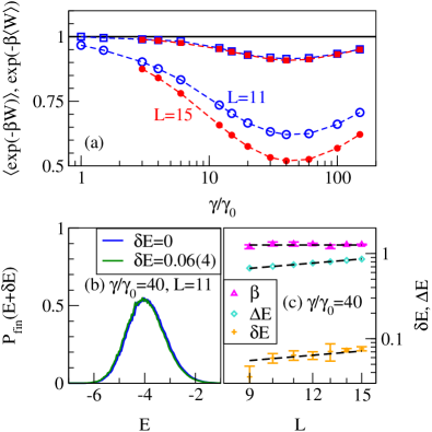
Figure 4: (a) Averages $\langle e^{-\beta W}\rangle$ (squares) and $e^{-\beta\langle W\rangle}$ (circles) as a function of the process rate $\gamma$ for two different $L=11,15$ and initial energies corresponding to the inverse temperature $\beta\approx 1.2$. (b) Final distribution $P_{\text{fin}}(E)$ and fictitious distribution $P_{\text{fin}}(E+\delta E)$ for $L=11$ and the rate $\gamma=40\,\gamma_{0}$, where the deviation of $\langle e^{-\beta W}\rangle$ from $1$ is largest in (a). (c) Finite-size scaling of $\beta$, $\Delta E$, and $\delta E$ for the $\gamma$ in (b). All error bars indicated in (b) correspond to errors resulting when determining $\beta$ by fitting locally the DOS.

Let us compare this result against the JR which here, since initial and final Hamiltonian are the same, reads

$$\langle e^{-\beta W}\rangle=\int P_{W}(W)\,e^{-\beta W}\,\text{d}W=1\,.$$ (7)

If the initial state was a true energy eigenstate at energy $E=E_{\text{ini}}$, then it would be justified to infer the actual probability distribution of work $P_{W}$ from $P_{\text{fin}}$ as $P_{W}(W)=P_{\text{fin}}(W+E_{\text{ini}})$. In this case the latter expression could be used to check Eq. (7) directly. Given the “narrowness” of $P_{\text{ini}}$, it seems plausible that the actual work-probability distribution $P_{W}(W)$ must be close to $P_{\text{fin}}(W+E_{\text{ini}})$. However, since $P_{\text{ini}}$ is not precisely a $\delta$-distribution, one cannot, strictly speaking, conclude from $P_{\text{fin}}$ onto $P_{W}$. To nonetheless do so, we employ a further assumption, namely, that the true $P_{W}$ computed from an actual initial $\delta$-function would not change much under variation of the position of the initial $\delta$-peak on the order of the width of $P_{\text{ini}}$, i.e., $\approx 0.25J_{\parallel}$. Under this assumption, the l.h.s. of Eq. (7) may be cast into the form SM

$$\frac{\int P_{\text{fin}}(E_{\text{fin}})\,e^{-\beta E_{\text{fin}}}\,\text{d}E_{\text{fin}}}{\int P_{\text{ini}}(E_{\text{ini}})\,e^{-\beta E_{\text{ini}}}\,\text{d}E_{\text{ini}}}=\int P_{W}(W)\,e^{-\beta W}\,\text{d}W\,.$$ (8)

Thus, the l.h.s. of Eq. (8) yields $\langle e^{-\beta W}\rangle$ based on $P_{\text{fin}},P_{\text{ini}}$ for different sweep rates $\gamma$. The closeness of the outcome to $1$ indicates how well the JR is fulfilled. As shown in Fig. 4, for very slow processes the l.h.s. of Eq. (8) is practically $1$, while there is a difference of ca. $0.1$ for faster processes. Comparing this difference to the deviation of $e^{-\beta\langle W\rangle}$ from $1$, points to the approximate validity rather than a strong violation of the JR.

To judge further on this, we use the following scheme: For every actual $P_{\text{fin}}(E_{\text{fin}})$ there is a fictitious probability distribution ${\cal P}(E_{\text{fin}}):=P_{\text{fin}}(E_{\text{fin}}+\delta E)$, which is identical in shape but shifted in energy by $\delta E$ and fulfills the JR exactly, i.e., Eq. (8) with $P_{\text{fin}}\rightarrow{\cal P}$ is identical to 1. We use this equation to identify $\delta E$ and get $\delta E=0.06(4)$ for $L=11$ and for $\gamma=40\gamma_{0}$ where the deviation of the l.h.s. of Eq. (8) from $1$ is largest. In Fig. 4 (b) we display ${\cal P}(E_{\text{fin}})$ together with $P_{\text{fin}}(E_{\text{fin}})$. Clearly, the difference is hardly visible as $\delta E$ is much smaller than the standard deviation $\Delta E=0.7(4)$ of either distribution. Thus, while the JR is clearly violated, the smallness of $\delta E$ indicates that this violation is remarkably small.

It should be stressed that the JR exponentially amplifies errors in the negative tail of the distribution Halpern and Jarzynski (2006), i.e., a tiny lack of statistics in this tail can in principle result in a large deviation from the JR (the observed non-negativity of $\delta E$ probably reflects this occurrence). This implies that one needs roughly an exponential number of samples to get a good estimate of the average exponentiated work Jarzynski (2006) even for initial canonical states. In this sense the observed deviation from the JR of at most $10\%$, obtained from a single wave function, is indeed small and a central result of our Letter.

For all other sweep rates, $\delta E$ turns out to be even smaller, thus rendering the actual work-probability distribution even closer to the fictitious one. Note that the fictitious probability distribution ${\cal P}(E_{\text{fin}})$ introduced is certainly not the only choice possible. However, it allows for a very natural interpretation.

Finite-size scaling. Finally, we perform a finite-size scaling for $L=9,\ldots,15$ and $E_{\text{ini}}=-0.42(L-1)$, yielding $\beta\approx 1.2$ within the attainable precision. Focusing on $\gamma=40\gamma_{0}$ with the largest violation of the JR, we depict the scaling $\Delta E(L)$ and $\delta E(L)$ in Fig. 4 (c). While $\Delta E(L)$ follows a “trivial” upscaling $\Delta E(L)\propto\sqrt{L}$ SM , giving a precise statement on $\delta E(L)$ remains challenging. Given the error bars shown, resulting from errors when determining $\beta$ by fitting SM , a very reasonable guess is $\delta E(L)\propto\sqrt{L}$ and indicated in Fig. 4 (c). Then, $\delta E(L)/\Delta E(L)=\text{const}.$ and we can expect that the JR remains valid to very good approximation for $L\to\infty$. This is another central result of our work.

Conclusions. In summary, we have studied the validity of the JR for non-canonical initial states that are pure states close to energy eigenstates. To this end, we have performed large-scale numerics to first prepare typical states of such kind and then to propagate these states under a time-dependent protocol in a complex quantum system of condensed-matter type. While we have found violations of the JR in our non-equilibrium scenario, we have demonstrated that these violations are remarkably small and point to the approximative validity of the JR in a moderately sized system already. Furthermore, our systematic finite-size analysis has not shown indications that this result changes in the thermodynamic limit of very large systems.

While this result cannot be simply explained by the equivalence of ensembles, it indicates the validity of the ETH for a non-trivial operator being the “operator of exponentiated work”. This validity is surprising due to the structure of this operator but also since the ETH is commonly associated with equilibrium properties, while the JR addresses non-equilibrium processes. Promising directions of future research include the generality of our findings for a wider class of systems and protocols, the necessity of the two-measurement scheme, as well as the dependence of the work distribution as such on the type of initial condition realized.

Acknowledgements. The authors gratefully acknowledge the computing time granted by the JARA-HPC Vergabegremium and provided on the JARA-HPC Partition part of the supercomputer JUQUEEN Stephan and Docter (2015) at Forschungszentrum Jülich. We are thankful for valuable insights and fruitful discussions at working group meetings of the COST action MP1209.

I Supplemental material

I.1 Time-dependent Schrödinger equation

The full Hamiltonian of the spin-$1/2$ ladder system reads ${\cal H}(t)=H+h(t)$, where $H$ and $h(t)$ are defined by Eqs. (4) and (5) in the main text. Here, to shorten notation, we write ${\cal H}(t)$ instead of $H_{\text{tot}}(t)$. The time evolution of the system is governed by the time-dependent Schrödinger equation (TDSE) (in units of $\hbar=1$)

$$i\frac{\partial}{\partial t}|\Psi(t)\rangle={\cal H}(t)|\Psi(t)\rangle\,,$$ (9)

where $|\Psi(t)\rangle$ is the wave function of the system. The solution of the TDSE can be written as

$$|\Psi(t+\delta t)\rangle = U(t+\delta t,t)\,|\Psi(t)\rangle$$ (10)

$$= \exp_{+}\left(-i\int_{t}^{t+\delta t}{\cal H}(u)\,\text{d}u\right)\,|\Psi(t)\rangle,$$ (11)

where $\delta t$ is the time step. For small $\delta t$, the Hamiltonian is considered to be fixed in the time interval $[t,t+\delta t]$ and then the time-evolution operator may be approximated by

$$U(\delta t)=U(t+\delta t,t)=\exp(-i{\cal H}(t+\delta t/2)\delta t)\,.$$ (12)

We solve the TDSE using a second-order product-formula algorithm De Raedt (1987); De Raedt and Michielsen (2006). The basic idea of the algorithm is to use a second-oder approximation of the time-evolution operator $U(\delta t)$, given by

$$\widetilde{U}_{2}(\delta t)=e^{-i\delta t{\cal H}_{k}/2}\cdots e^{-i\delta t{\cal H}_{1}/2}e^{-i\delta t{\cal H}_{1}/2}\cdots e^{-i\delta t{\cal H}_{k}/2}\,,$$ (13)

where ${\cal H}={\cal H}_{1}+\cdots+{\cal H}_{k}$. The approximation is bounded by

$$||U(\delta t)-\widetilde{U}_{2}(\delta t)||\ll c_{2}\,\delta t^{3}\,,$$ (14)

where $c_{2}$ is a positive constant.

In practice, we use an XYZ decomposition for the Hamiltonian according to the $x$, $y$, and $z$ components of the spin operators, i.e., ${\cal H}={\cal H}_{x}+{\cal H}_{y}+{\cal H}_{z}$. The computational basis states are eigenstates of the $S^{z}$ operators. Thus, in this representation $e^{-i\delta t{\cal H}_{z}}$ is diagonal by construction, and it only changes the input state by altering the phase of each of the basis vectors. By an efficient basis rotation into the eigenstates of the $S^{x}$ or $S^{y}$ operators, the operators $e^{-i\delta t{\cal H}_{x}}$ and $e^{-i\delta t{\cal H}_{y}}$ act as $e^{-i\delta t{\cal H}_{z}}$.

I.2 Initial state

The initial state is obtained by a Gaussian projection of a random state drawn at random according to the Haar measure on the total Hilbert space of the system,

$$|\Psi(a,E)\rangle=\frac{e^{-a(H-E)^{2}/4}\,|\Phi\rangle}{\langle\Phi|\,e^{-a(H-E)^{2}/2}\,|\Phi\rangle}\,,$$ (15)

where $1/a$ characterizes the variance of the Gaussian projection and $H$ is the Hamiltonian at $t=0$. This calculation is performed by employing the Chebyshev-polynomial representation of a Gaussian function, properly generalized to matrix-valued functions Tal-Ezer and Kosloff (1984); Dobrovitski and De Raedt (2003), and yields numerical results which are accurate to about $14$ digits.

In general, a function $f(x)$ whose values are in the range $[-1,1]$ can be expressed as

$$f(x)=\frac{1}{2}c_{0}T_{0}(x)+\sum_{k=1}^{\infty}c_{k}T_{k}(x)\,,$$ (16)

where $T_{k}(x)=\cos(k\arccos x)$ are Chebyshev polynomials and the coefficients $c_{k}$ are given by

$$c_{k}=\frac{2}{\pi}\int_{-1}^{1}\frac{\text{d}x}{\sqrt{1-x^{2}}}\,f(x)\,T_{k}(x)\,.$$ (17)

Let $x=\cos\theta$, then $T_{k}(x)=\cos(k\theta)$ and

$$c_{k} = \frac{2}{\pi}\int_{0}^{\pi}f(\cos\theta)\cos(k\theta)\,\text{d}\theta$$ (18)

$$= \text{Re}\left[\frac{2}{N}\sum_{n=0}^{N-1}f\left(\cos\frac{2\pi n}{N}\right)e^{2\pi ink/N}\right]\,,$$ (19)

which can be calculated by the fast Fourier transform (FFT).

For the operators $f(H)=e^{-a(H-E)^{2}/4}$, we normalize $H$ such that $\widetilde{H}=H/||H||$ has eigenvalues in the range $[-1,1]$ and put $\widetilde{a}=a||H||$ and $\widetilde{E}=E/||H||$. Then

$$f(\widetilde{H})=e^{-\widetilde{a}(\widetilde{H}-\widetilde{E})^{2}/4}=\sum_{k=0}^{\infty}c_{k}T_{k}(\widetilde{H})\,,$$ (20)

where $\{c_{k}\}$ are the Chebyshev-expansion coefficients calculated from Eq. (19) and the Chebyshev polynomial $T_{k}(\widetilde{H})$ can be obtained by the recursion relation

$$T_{k+1}(\widetilde{H})-2\widetilde{H}T_{k}(\widetilde{H})+T_{k-1}(\widetilde{H})=0$$ (21)

with $T_{0}(\widetilde{H})=1$ and $T_{1}(\widetilde{H})=\widetilde{H}$.

In practice, the coefficients $c_{k}$ become exactly zero for a certain $k\geq K$. Hence, we have an exact representation of the Gaussian projection up to a sum of $K$ terms in Eq. (20). Note that the Chebyshev algorithm can only be efficiently applied to solve the TDSE if the total Hamiltonian is time-independent Dobrovitski and De Raedt (2003).

I.3 Density of states

The density of states (DOS) of a quantum system may, on the basis of a time evolution, be defined as

$$n(E)=\sum_{n}\delta(E-E_{n})=\frac{1}{2\pi}\int_{-\infty}^{+\infty}e^{itE}\,\text{Tr}\{e^{-itH}\}\,\text{d}t\,,$$ (22)

where $H$ is the Hamiltonian of the system at $t=0$ and $n$ runs over all eigenvalues $E_{n}$ of $H$. The trace in the integral can be estimated from the expectation value with respect to a random vector, e.g., by exploiting quantum typicality Hams and De Raedt (2000b); Steinigeweg et al. (2014c). Thus, we have

$$\frac{\text{Tr}\{e^{-itH}\}}{D}\approx\langle\Phi(0)|e^{-itH}|\Phi(0)\rangle=\langle\Phi(0)|\Phi(t)\rangle\,,$$ (23)

where $D$ is the dimension of the Hilbert space and $|\Phi(0)\rangle$ is a pure state drawn at random according to the unitary invariant measure (Haar measure) and the error scales with $1/\sqrt{D}$. $|\Phi(t)\rangle=e^{-itH}|\Phi(0)\rangle$ can be efficiently computed by the second-oder product-formula algorithm. Therefore, the DOS can be conveniently calculated by FFT,

$$n(E)\approx C\int_{-\Theta}^{+\Theta}e^{itE}\langle\Phi(0)|\Phi(t)\rangle\text{d}t\,,$$ (24)

where $C$ is a normalization constant and $\Theta$ is the time up to which one has to integrate the TDSE in order to reach the desired energy resolution $\pi/\Theta$. The Nyquist sampling theorem gives an upper bound to the time-step that can be used. For the systems considered in the present paper, this bound is sufficiently small to guarantee that the errors on the eigenvalues are small, see Ref. Hams and De Raedt (2000b) for a derivation of bounds, etc.

Similarly, we can obtain the local DOS (LDOS) of the system for a particular pure state $|\Psi\rangle$, such as the initial state and final state of the system, by the formula

$$P(E) = \sum_{n}d_{n}^{2}\,\delta(E-E_{n})=\sum_{n}|\langle E_{n}|\Psi\rangle|^{2}\,\delta(E-E_{n})$$ (25)

$$= \frac{1}{2\pi}\int_{-\infty}^{+\infty}e^{itE}\,\langle\Psi|\,e^{-itH}\,|\Psi\rangle\,\text{d}t$$ (26)

$$\approx C\int_{-\Theta}^{+\Theta}e^{itE}\,\langle\Psi|\,e^{-itH}\,|\Psi\rangle\,\text{d}t\,,$$ (27)

where $|E_{n}\rangle$ are energy eigenstates and $d_{n}=\langle E_{n}|\Psi\rangle$. Note that the concept of typicality is not involved in the calculation of $P(E)$.

I.4 Numerical simulation

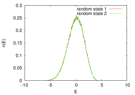
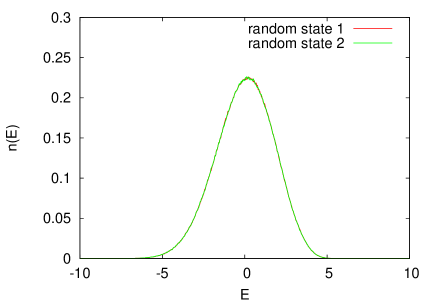
Figure 5: Simulation results for the density of states $n(E)$ for a quantum ladder system with $18$ spins (top) and $22$ spins (bottom). Two different random states are used to compute $n(E)$ according to the algorithm described in the text. The system Hamiltonian is defined by Eq. (4) in the main text.

The algorithm to compute the DOS $n(E)$ consists of the following steps:

1. Generate a random state $|\Phi(0)\rangle$ at $t=0$.

2. Copy this state to $|\Phi(t)\rangle$.

3. Calculate $\langle\Phi(0)|\Phi(t)\rangle$ and store the result.

4. Solve the TDSE for a small time step $\delta t$, replacing $|\Phi(t)\rangle$ by $|\Phi(t+\delta t)\rangle$.

5. Repeat $K$ times step $3$ and $4$.

6. Perform a Fourier transform on the tabulated result.

In the simulation, we use $\delta t=0.02$ for the second-order product-formula algorithm and repeat $K=4096\times 5$ steps. The total simulation time is $\Theta=409.6$. Hence, the energy resolution is about $\pi/\Theta\approx 0.0077$. In principle, $n(E)$ may be averaged over different random states. It turns out that this is only necessary for small system sizes as the error scales with the square root of the dimension of the Hilbert space. Figure 5 shows the simulation results for $n(E)$ obtained from two different random states for systems with $18$ and $22$ spins. It can be clearly seen that the curves $n(E)$ obtained for two different random states coincide apart from some small fluctuations. These fluctuations disappear for larger system sizes.

The strategy for numerically testing the Jarzynski relation is:

1. Generate the initial state $|\Psi(a,E_{\text{ini}},t=0)\rangle$ by the Chebyshev polynomial algorithm.

2. Calculate the LDOS $P_{\text{ini}}(E)$ for the initial state $|\Psi(a,E_{\text{ini}},t=0)\rangle$.

3. Solve the TDSE for the time-dependent Hamiltonian $H+h(t)$.

4. Calculate the LDOS $P_{\text{fin}}(E)$ for the final state $|\Psi(a,E_{\text{ini}},t=2\tau)\rangle$.

5. Repeat from step $3$ for different process rates $\gamma=1/2\tau$.

In the simulation, the parameters for the initial states are $a=1000$ and $E_{\text{ini}}=0.42(L-1)$, $L=N/2$, where $N$ ranges from $18$ to $30$. We use $\delta t=0.02$ for the second-order product-formula algorithm to solve the TDSE. After the whole process, we collect the data sets of $n(E)$, $\langle E\rangle_{\text{ini}}$, $P_{\text{ini}}(E)$, $\langle E\rangle_{\text{fin}}$, and $P_{\text{fin}}(E)$ for further analysis.

Our goal is to test the validity of the Jarzynski relation beyond the Gibbsian initial state in isolated systems, i.e.,

$$\langle e^{-\beta W}\rangle=\int P_{\text{W}}(W)\,e^{-\beta W}\,\text{d}W=e^{-\beta\Delta F}\,,$$ (28)

where the work $W$ is defined as $W=E_{\text{fin}}-E_{\text{ini}}$ according to the two-measurement scheme, $P_{\text{W}}(W)$ is the work probability, and $\Delta F$ is the difference between the free energies of the two equilibrium states of the initial and final Hamiltonian. Obviously, we need to calculate both sides of Eq. (28). The right-hand side equals $1$ as the protocol we uses (see Eq. (5) in the main text) ends with the same Hamiltonian as the initial one and hence $\Delta F=0$. Therefore, we only need to calculate the left-hand side, which requires the information about the inverse temperature $\beta$ and the work probability $P_{\text{W}}(W)$.

I.4.1 Estimation of the inverse temperature $\beta$

The initial state is narrowly centered at the initial energy $E_{\text{ini}}$ (as the standard deviation of $P_{\text{ini}}(E)$ is about $0.03$ for $a=1000$). A microcanonical temperature can be calculated according to the standard formula

$$\beta=\frac{\text{d}S}{\text{d}E}\,,$$ (29)

where $S=\ln n(E)$ is the microcanonical entropy.

We get $\beta$ from fitting $n(E)$ in the interval $[E_{\text{ini}}-\epsilon,E_{\text{ini}}+\epsilon]$, where $E_{\text{ini}}$ is the initial mean energy and $\epsilon$ is a parameter to determine the range for fitting. The inverse temperature $\beta$ does not vary significantly for $\epsilon\lesssim 0.5$ (see below).

I.4.2 Estimation of the work probability $P_{\text{W}}(W)$

As mentioned in the main text, we have two non-trivial distributions of energy, a final and an initial one, from which $P_{W}$ must be inferred. Without further assumptions, the attribution of a final and an initial distribution of energy to one distribution of work cannot be entirely unique. Thus, we rely on a further assumption: The probability distribution of work as arising from an initial $\delta$ distribution w.r.t. energy could in principle vary strongly with the position $E_{\text{ini}}$ at which this initial distribution is peaked. Assuming that this is not the case on the small regime where $P_{\text{ini}}(E)$ takes on non-negligible values, the probability distributions of work and energy are related as

$$P_{\text{fin}}(E_{\text{fin}})=\int P_{\text{ini}}(E_{\text{ini}})\,P_{W}(E_{\text{fin}}-E_{\text{ini}})\,\text{d}E_{\text{ini}}\,.$$ (30)

Multiplying this equation by $e^{-\beta}E_{\text{fin}}$ and integrating over $E_{\text{fin}}$, followed by a change of variables $E_{\text{fin}}\rightarrow W+E_{\text{ini}}$ on the r.h.s. yields

$$\frac{\int P_{\text{fin}}(E_{\text{fin}})\,e^{-\beta E_{\text{fin}}}\,\text{d}E_{\text{fin}}}{\int P_{\text{ini}}(E_{\text{ini}})\,e^{-\beta E_{\text{ini}}}\,\text{d}E_{\text{ini}}}=\int P_{\text{W}}(W)\,e^{-\beta W}\,\text{d}W\,.$$ (31)

Thus, the l.h.s. of Eq. (31) yields $\langle e^{-\beta W}\rangle$ based on $P_{\text{fin}},P_{\text{ini}}$ for different sweep rates $\gamma$.

I.4.3 Estimations of $\langle e^{-\beta W}\rangle$ and $e^{-\beta\langle W\rangle}$

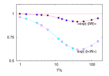
Figure 6: Simulation results for $\langle e^{-\beta W}\rangle$ and $e^{-\beta\langle W\rangle}$ as a function of the process rate $\gamma$ (normalized to the slowest rate $\gamma_{0}=2.6\times 10^{-4}$) for two different random states $|\Phi\rangle$ (represented by squares and circles) used to determine the initial states (see Eq. (15)). The system is a quantum ladder with $22$ spins. The initial energy corresponds to the inverse temperature $\beta=1.23$ (see Fig. 2 (inset) in the main text).

In order to calculate the left-hand side of Eq. (28), i.e., $\langle e^{-\beta W}\rangle$, we do not have to really calculate the work probability. As explained before, the left-hand side can be expressed as

$$\langle e^{-\beta W}\rangle=\frac{\int P_{\text{fin}}(E_{\text{fin}})\,e^{-\beta E_{\text{fin}}}\,\text{d}E_{\text{fin}}}{\int P_{\text{ini}}(E_{\text{ini}})\,e^{-\beta E_{\text{ini}}}\,\text{d}E_{\text{ini}}}\,.$$ (32)

Similarly, we have

$$\langle W\rangle = \int P_{\text{fin}}(E_{\text{fin}})\,{E_{\text{fin}}}\,\text{d}E_{\text{fin}}-\int P_{\text{ini}}(E_{\text{ini}})\,{E_{\text{ini}}}\,\text{d}E_{\text{ini}}$$ (33)

$$= \langle E_{\text{fin}}\rangle-\langle E_{\text{ini}}\rangle$$ (34)

and

$$e^{-\beta\langle W\rangle}=e^{-\beta(\langle E_{\text{fin}}\rangle-\langle E_{\text{ini}}\rangle)}\,.$$ (35)

Hence, the calculations of $\langle e^{-\beta W}\rangle$ and $e^{-\beta\langle W\rangle}$ solely depend on the data set obtained from the simulation.

Figure 6 presents the simulation results for $\langle e^{-\beta W}\rangle$ and $e^{-\beta\langle W\rangle}$ as a function of the process rate of the magnetic field imposed on the two legs of the ladder for $22$ spins. The inverse temperature $\beta$ is set to $1.23$ (see Fig. 2 in the main text). Two different random states are used to prepare the initial state of the system. It can be seen that $\langle e^{-\beta W}\rangle$ and $e^{-\beta\langle W\rangle}$ calculated for these two different initial states do not differ much. Hence, it is sufficient to study the Jarzynski relation only for one particular initial state.

I.4.4 Error estimation of $\langle e^{-\beta W}\rangle$

The main error of our overall analysis is set neither by our numerical methods (finite time step, maximum time) nor by the specific realization of the initial state. Instead, the main error results when determining the inverse temperature $\beta$ by fitting locally the density of states. By varying the fit range $[E_{\text{ini}}-\epsilon,E_{\text{ini}}+\epsilon]$ from $\epsilon=0.25$ to $\epsilon=0.5$, we find that the value of $\beta$ can be determined with a precision of $\approx 5\,\%$, see the small error bars in Fig. 4 (c) of the main text. This precision implies that, for the sweep rate $\gamma/\gamma_{0}=40$, the quantity $\langle e^{-\beta W}\rangle$ has a corresponding error of $\approx 2\,\%$. This error is smaller than the symbol size used and not indicated explicitly in Fig. 4 (a) of the main text. We can therefore exclude that the deviation of this quantity from $1$ for such values of $\gamma$ is an artifact of our approach.

However, the corresponding error for the shift $\delta E$ is much larger since

$$\delta E=-\frac{1}{\beta}\,\ln\langle e^{-\beta W}\rangle$$ (36)

essentially is the logarithm of a small number $<1$. Consequently, the corresponding error can be as large as $\approx 30\,\%$, see the error bars in Fig. 4 (c) of the main text. Such errors of $\delta E$ are particularly relevant for the quality of the finite-size scaling $\delta E(L)$ and thus taken into account in the conclusions.

I.5 Finite-size scaling

A central result of our Letter concerns the upscaling of the system towards the limit $L\rightarrow\infty$. It is instructive to compare to a set of $M$ disconnected small systems: The work-probability distribution in this case is a $M$-fold convolution of the work-probability distribution as resulting for each small system. Since mean values are additive under convolution, one gets the corresponding shift scaling as $\delta E(M)=M\delta E(1)$. The standard deviation of the work-probability distribution, however, scales under convolution as $\Delta E(M)=\sqrt{M}\Delta E(1)$. This implies that, for large $M$, $\delta E(M)$ becomes inevitably larger than $\Delta E(M)$ and thus the resulting work-probability distribution is far away from fulfilling the JR. Therefore, in the limit of many disconnected small systems, the JR is strongly violated whenever $\delta E(1)$ is non-zero. This finding is clearly different to a long connected ladder, as discussed in our Letter.

References

- Popescu et al. (2006) S. Popescu, A. J. Short, and A. Winter, Nature Phys. 2, 754 (2006).
- Goldstein et al. (2006) S. Goldstein, J. L. Lebowitz, R. Tumulka, and N. Zanghì, Phys. Rev. Lett. 96, 050403 (2006).
- Reimann (2008) P. Reimann, Phys. Rev. Lett. 101, 190403 (2008).
- Reimann (2015) P. Reimann, Phys. Rev. Lett. 115, 010403 (2015).
- Eisert et al. (2015) J. Eisert, M. Friesdorf, and C. Gogolin, Nature Phys. 11, 124 (2015).
- Gogolin and Eisert (2015) C. Gogolin and J. Eisert, arXiv:1503.07538 (2015).
- Rigol et al. (2008) M. Rigol, V. Dunjko, and M. Olshanii, Nature 854, 452 (2008).
- Steinigeweg et al. (2013) R. Steinigeweg, J. Herbrych, and P. Prelovšek, Phys. Rev. E 87, 012118 (2013).
- Beugeling et al. (2014) W. Beugeling, R. Moessner, and M. Haque, Phys. Rev. E 89, 042112 (2014).
- Steinigeweg et al. (2014a) R. Steinigeweg, A. Khodja, H. Niemeyer, C. Gogolin, and J. Gemmer, Phys. Rev. Lett. 112, 130403 (2014a).
- Malabarba et al. (2014) A. S. L. Malabarba, L. P. García-Pintos, N. Linden, T. C. Farrelly, and A. J. Short, Phys. Rev. E 90, 012121 (2014).
- Reimann (2016) P. Reimann, Nat. Com. 7, 10821 (2016).
- Niemeyer et al. (2014) H. Niemeyer, K. Michielsen, H. De Raedt, and J. Gemmer, Phys. Rev. E 89, 012131 (2014).
- Gemmer and Steinigeweg (2014) J. Gemmer and R. Steinigeweg, Phys. Rev. E 89, 042113 (2014).
- Schmidtke and Gemmer (2016) D. Schmidtke and J. Gemmer, Phys. Rev. E 93, 012125 (2016).
- Seifert (2008) U. Seifert, Eur. Phys. J. B 64, 423 (2008).
- Esposito et al. (2009) M. Esposito, U. Harbola, and S. Mukamel, Rev. Mod. Phys. 81, 1665 (2009).
- Jarzynski (2011) C. Jarzynski, Annu. Rev. Condens. Matter Phys. 2, 329 (2011).
- Roncaglia et al. (2014) A. J. Roncaglia, F. Cerisola, and J. P. Paz, Phys. Rev. Lett. 113, 250601 (2014).
- Hänggi and Talkner (2015) P. Hänggi and P. Talkner, Nature Phys. 11, 108 (2015).
- Talkner et al. (2008) P. Talkner, P. Hänggi, and M. Morillo, Phys. Rev. E 77, 051131 (2008).
- Campisi (2008) M. Campisi, Phys. Rev. E 78, 012102 (2008).
- Talkner et al. (2013) P. Talkner, M. Morillo, J. Yi, and P. Hänggi, New J. Phys. 15, 095001 (2013).
- Campisi et al. (2011) M. Campisi, P. Hänggi, and P. Talkner, Rev. Mod. Phys. 83, 771 (2011).
- (25) Here, we assume that the spectrum is non-degenerate.
- Srednicki (1994) M. Srednicki, Phys. Rev. E 50, 888 (1994).
- Deutsch (1991) J. M. Deutsch, Phys. Rev. A 43, 2046 (1991).
- (28) See supplemental materials for details.
- Hams and De Raedt (2000a) A. Hams and H. De Raedt, Phys. Rev. E 62, 4365 (2000a).
- Steinigeweg et al. (2014b) R. Steinigeweg, J. Gemmer, and W. Brenig, Phys. Rev. Lett. 112, 120601 (2014b).
- Steinigeweg et al. (2016) R. Steinigeweg, J. Herbrych, X. Zotos, and W. Brenig, Phys. Rev. Lett. 116, 017202 (2016).
- Halpern and Jarzynski (2006) N. Y. Halpern and C. Jarzynski, arXiv:1601.02637 (2006).
- Jarzynski (2006) C. Jarzynski, Phys. Rev. E 73, 046105 (2006).
- Stephan and Docter (2015) M. Stephan and J. Docter, J. Large-Scale Research Facilities 1, A1 (2015).
- De Raedt (1987) H. De Raedt, Comp. Phys. Rep. 7, 1 (1987).
- De Raedt and Michielsen (2006) H. De Raedt and K. Michielsen, in Handbook of Theoretical and Computational Nanotechnology, edited by M. Rieth and W. Schommers (American Scientific Publishers, Los Angeles, 2006) pp. 2 – 48.
- Tal-Ezer and Kosloff (1984) H. Tal-Ezer and R. Kosloff, J. Chem. Phys. 81, 3967 (1984).
- Dobrovitski and De Raedt (2003) V. V. Dobrovitski and H. De Raedt, Phys. Rev. E 67, 056702 (2003).
- Hams and De Raedt (2000b) A. Hams and H. De Raedt, Phys. Rev. E 62, 4365 (2000b).
- Steinigeweg et al. (2014c) R. Steinigeweg, A. Khodja, H. Niemeyer, C. Gogolin, and J. Gemmer, Phys. Rev. Lett. 112, 130403 (2014c).